
Submitted:
08 April 2025
Posted:
09 April 2025
You are already at the latest version
Abstract
One of the most challenging tasks in studying precipitation is quantifying how the complexities of individual components contribute to the overall system complexity. To address this, we employed information measures based on Kolmogorov complexity (KC), specifically the Kolmogorov complexity spectrum (KC spectrum) and the Kolmogorov complexity plane (KC plane). We applied these measures to monthly time series data, both measured and simulated by the EBU POM regional climate model, spanning the period from 1982 to 2005 for Sombor (45.78°N, 19.12°E) in Serbia. The variables analyzed included precipitation—a complex physical system—and its individual components: mean temperature, minimum and maximum temperatures, humidity, wind speed, and global radiation. By applying the listed measures to the all-time series, we calculated normalized KC spectra for each position in the KC plane, displaying interactive master amplitudes against individual amplitudes. We proposed a simplified four-step method to compute the relative change in complexities within the overlapping area beneath the KC spectra. Our results facilitated a discussion on the relationship between the complexity of precipitation and that of its individual components.
Keywords:
Precipitation
; Kolmogorov complexity (KC)
; KC spectrum
; KC plane
; dynamic and thermodynamic of atmosphere
; overlapping spectra in discrete form
; hierarchy in complex systems
1. Introduction
Understanding precipitation patterns is essential for a wide range of fields, including meteorology, agriculture, and climate science. However, traditional approaches to studying precipitation often depend on linear models and historical data analysis, which can fail to capture the intricate interactions and dynamic complexities inherent in weather systems.
1.1. Preliminaries
Precipitation is a multifaceted phenomenon that exhibits several key characteristics of a complex system: (1) Interconnected processes: Cloud formation is a prime example, where atmospheric conditions, aerosol presence, and temperature gradients interact to influence precipitation development. (2) Atmospheric dynamics: Wind patterns, temperature gradients, and humidity levels are crucial in shaping cloud development and precipitation distribution. These factors interact in complex ways to determine where and when precipitation occurs. (3) Feedback loops: Processes such as evaporation and condensation create feedback loops that significantly affect precipitation intensity and distribution. For instance, increased evaporation can lead to more intense precipitation events. (4) Nonlinearity: Small changes in atmospheric conditions can lead to substantial variations in precipitation patterns, illustrating the system's sensitivity to initial conditions. (5) Emergence: The collective behavior of atmospheric particles and processes gives rise to emergent properties, such as complex precipitation patterns, which cannot be predicted solely from the characteristics of their components. Note that this emergent behavior is a hallmark of complex systems. (6) Adaptation and sensitivity: Precipitation systems are susceptible to fluctuations in global climate patterns, such as El Niño and the North Atlantic Oscillation. These fluctuations can profoundly impact regional precipitation patterns, leading to significant alterations in local hydrological cycles, and (7) Scale and hierarchy: Precipitation phenomena unfold across multiple spatial and temporal scales, ranging from localized thunderstorms to large-scale global climate patterns. To fully grasp precipitation, it is essential to consider these diverse scales and their intricate interactions.
Therefore, precipitation constitutes a complex physical system characterized by interconnected processes, nonlinear dynamics, emergent properties, heightened sensitivity to environmental changes, a hierarchical structure spanning multiple scales, and an inherently interdisciplinary nature that necessitates a comprehensive, multifaceted approach to its study.
1.2. Complexity Versus Randomness
In the previous subsection, we discussed the properties of precipitation as a complex system. When considering the complexity of this system and its implications for precipitation, two key points should be kept in mind: (1) Defining complexity: While there is ongoing debate regarding the precise definition of complexity as a property of complex systems, it is typically quantified using various complexity measures derived from analyzed time series data. (2) Complexity vs. randomness: It is important to note that complexity should not be conflated with randomness. Complexity involves structured interactions and patterns, whereas randomness implies a lack of discernible order or predictability.
As illustrated in Figure 1, a system is either highly ordered (e.g., crystal) or highly random (e.g., gas). Both of them are systems of low complexity. In reality, any complex system showsthe coexistence of both regularity and randomness. Complete randomness does not imply a total absence of patterns. In theory, truly random sequences can exhibit apparent patterns due to the probabilistic nature of randomness and the limitations of observing finite sequence lengths [3]. However, if a sequence is genuinely random, these patterns should lack predictability and consistency over time. To avoid confusion, it is worth noting the distinction between the phrases "complexity of precipitation" and "precipitation complexity," which are often used interchangeably. However, there can be a subtle difference in emphasis depending on the context. The phrase "complexity of precipitation" tends to emphasize the inherent complexities within the phenomenon of precipitation itself. It highlights the intricate processes, mechanisms, and factors influencing precipitation, such as atmospheric conditions, cloud dynamics, and global climate patterns. On the other hand, "precipitation complexity" might be interpreted as emphasizing the complexity that arises from precipitation, referring to the impact on systems, environments, or societies, and highlighting how precipitation contributes to or interacts with broader complex systems.
It is important to note that discrepancies in complexity patterns between different states of a complex system can arise from a common misconception: equating complexity with entropy. While entropy algorithms can provide estimates of complexity, these values are inherently dependent on the specific algorithm used and should not be considered as direct measures of complexity. For example, in the context of brain signals, high randomness might intuitively suggest decreased complexity due to the lack of structured patterns. However, when using common entropy algorithms to measure brain entropy, the results often show an opposite trend. This is illustrated in Figure 2a and 2b, where increased randomness in brain signals leads to higher entropy values despite the actual complexity potentially decreasing.
Numerous researchers have investigated the relationship between complexity and precipitation, utilizing entropy measures and traditional statistical techniques in their analyses ([5,6,7], among many others). In contrast to previous approaches, this issue can be addressed through an alternative framework, employing two innovative measures of complexity: the Kolmogorov Complexity Spectrum (KC spectrum) and the Kolmogorov complexity plane of interacting amplitudes (KC plane). The KC Plane facilitates the identification of specific intervals of interacting amplitudes, where the contributions of individual meteorological elements' complexities to the overall complexity of precipitation can be quantified.
This paper investigates the relationship between the complexity of precipitation (master complexity) in Sombor (Serbia) in the period 1982–2005 and the combined complexities of meteorological components, specifically mean temperature, minimum/maximum temperatures, humidity, wind speed, and global radiation. The structure of this paper is as follows: Section 2 provides a brief methodological overview and details the data utilized. Section 3 presents and discusses the results. Section 4 outlines the conclusions derived from the study's findings.
2. Methodology: Information Measures and Data Used
Kolmogorov complexity.If a universal Turing machine generates the output, then the Kolmogorov complexity of a given object is defined as, which is the size of the shortest program that generates the object. , while for most objects. Since of an arbitrary object is incomputable, it is approximated by the Lempel-Ziv algorithm (LZA) [8] and its variants (see Appendix A [9]). The problem with the LZA algorithm is that it operates with binary time series.
Kolmogorov complexity spectra. If the LZA algorithm is applied times to a time series , using all elements of as thresholds forming the sequence, then the sequence is called the Kolmogorov complexity spectrum (KC spectrum) of a time series . This series is transformed into a string of finite symbols by comparison with a series of thresholds, where each element is equal to the corresponding element in the time series, applying the LZA algorithm. The original time series samples are converted into a set of 0–1 sequence defined by comparison with a threshold ,
After applying the LZA algorithm to each element of the series , we get the KC spectrum[9].
Kolmogorov complexity plane of interacting amplitudes. One of the most challenging tasks in studying complex physical systems is determining the contributions of the complexities of individual components to the complexity of the entire system. The Kolmogorov complexity plane of interacting amplitudes (KC plane) is a conceptual framework used to analyze the contributions of individual components to the overall complexity of a system. This approach, introduced by Mihailović et al. [10], employs the KC plane in a two-dimensional space (1,1) to study physical systems and their components through their respective complexities. The KC plane provides a robust method for analyzing complex systems by linking individual component behaviors to overall system dynamics. It allows researchers to pinpoint critical intervals of interaction between master and individual complexities, offering insights into emergent phenomena in self-organizing systems. To illustrate this concept, we will use time series data generated by the instrument, where . Here, is the amplitude factor, is a random number uniformly distributed over the interval [0,1], and the sampling interval is . The state space , consists of cells of size , sampled at each time point . The measurement time series is composed of successive elements.
A comparison of the two KC spectra is shown in Figure 3a, which represents two merged two-dimensional graphs (with different meanings of axes): (i) KC master vs. individual components (both amplitudes are on-axis and both complexities are on -axis) and (ii)(the master amplitude) vs. (individual amplitude), i.e., the KC plane. The black and red circles represent the master () and individual spectra (), which are calculated from the time series generated by a random generator. At the same time, squares mark points in the KC plane. These quantities were compared in a two-dimensional system scaled from 0 to 1, using normalized time series.
A comparison of the two KC spectra is shown in Figure 3, which represents two merged two-dimensional graphs (with different meanings of axes): (i) KC master vs. individual components (both amplitudes are on -axis and both complexities are on -axis) and (ii) (the master amplitude) vs. (individual amplitude), i.e., the KC plane. The black and red circles represent the master () and individual spectra (), which are calculated from the time series generated by a random generator (Figure 3a). At the same time, squares mark points in the KC plane. These quantities were compared in a two-dimensional system scaled from 0 to 1, using normalized time series. We can assess the relationships since these quantities are on the same scale after normalization. Since these quantities are on the same scale after normalization, we can assess relationships and patterns between the compared quantities without the influence of varying scales [11]. Further, from Figure 3a, the squares in the (, ) system are scattered. This is due to the dynamic relationship and interdependence between the "master"variant and individual ones. It can also be seen that there are two groups of points. One that belongs to the area under the spectrum curve (the set ), and another that belongs to the area under the spectrum curve (the set ). However, only points from the set defined as=∩ are the candidates for comparison of the complexity of different sequences or systems (in this case, the entire complex physical system and its components). The amplitudes that belong to this set will conditionally be called interactive amplitudes [10]. To evaluate points against both curves given in discrete forms, we used nonlinear curve comparison from the R packages. In the fitting procedure, the cubic spline method was used instead of the existing one. In evaluating the number of points in the set of the KC plane, some points may lie outside this set but are still counted among its points. However, in this paper, the number of such points does not exceed 0.05 percent of the total number of points in the KC plane.
The threshold of minimal change in KC indicating a shift in the complex systems (TKC). Our analysis of the relationship between overall complexity and individual complexities will be grounded in Kolmogorov complexity (KC) analyses, such as Lempel-Ziv complexity, within the set. This raises the question of what thresholds of minimal change in KC (TKC) signify a shift in complex systems. While there is no universal minimal KC threshold, relative changes reliably indicate systemic shifts in complex systems. Let's examine some practical threshold values derived from various studies. In cardiology, atrial fibrillation is associated with highly complex local electrical activity, as reflected in the rich morphology of intracardiac electrograms [12]. In this context, the authors used a TKC of 5%. For fluid dynamics, a change greater than 10% in the vertical distribution of KC or its spectrum can indicate a transition from steady to unsteady flow conditions, such as during the passage of an undular surge [13]. In meteorology, detecting minimal changes in KC that indicate significant shifts in complex systems—like weather patterns or climate dynamics—requires analyzing the KC spectrum. Changes in the smoothness or peak distribution of the KC spectrum can signal shifts in weather patterns. For example, low values may disrupt the spectrum's smoothness, reflecting increased complexity under certain conditions (e.g., partly cloudy conditions affecting solar radiation variability) when TKC exceeds 10% [14]. Kovalsky et al. [15] analyzed outputs from LIGO experiments—which fall under gravitational physics, specifically focusing on general relativity and gravitational-wave astronomy—using KC spectra of residual, raw, and template time series from the Hanford and Livingston observatories. Their analysis revealed valuable insights regarding the interval (0.02, 0.18) of KC, providing critical context for interpreting gravitational wave detection methodologies.
Data used. To test the proposed method, two types of datasets were utilized [observed (O) and climate simulation data (M)] for the city Sombor (45.78°N, 19.12°E) in Serbia. The analysis covered the period from 1982 to 2005. The observed dataset included monthly values for precipitation (PRE), mean temperature (Tav), minimum and maximum temperatures (Tmin and Tmax), wind speed (WS), and global radiation (GR), sourced from the Republic Hydrometeorological Institute of Serbia. The climate simulation data were generated using a dynamic downscaling technique with the EBU-POM model under the pessimistic SRES-A2 greenhouse gas emissions scenario. EBU-POM is an atmosphere-ocean regional coupled climate model [16], with horizontal resolutions of 0.25° for the atmospheric component and 0.2° for the oceanic component. The regional model simulations spanned the period 1961–2100, using initial and lateral boundary conditions derived from the ECHAM5/MPI-OM global climate model [17]. All time series were normalized as follows: Given a time series , normalization was performed using the transformation: where represents the original time series (either observed or simulated), is the maximum value in the series, and is the minimum value. This normalization ensures all values fall within a range of 0 to 1.
To compare the overall complexity of precipitation with the complexities of individual components (observed and modeled), we employed the normalized time series, which are illustrated in Figure 4, Figure 5 and Figure 6, respectively. Each time series comprised 288 samples. Table 1 summarizes the maximum and minimum values used for normalization of the time series data.
3. Results and Discussion
Initially, we will discuss the rationale behind selecting the aforementioned meteorological variables to analyze the complexity of precipitation. Temperature (mean/maximum minimum) directly influences atmospheric moisture content, determining the precipitation intensity and variability (thermodynamic effects).Temperature gradients influence atmospheric circulation patterns, which in turn affect vertical motion and precipitation formation processes (dynamic effects). Atmospheric humidity is a critical factor in precipitation potential. As humidity increases, it enhances convective stability, thereby elevating the risk of extreme precipitation events. Wind speed is essential for transporting moisture and affecting convergence zones, where the conditions are favorable for precipitation to form. Solar radiation is a key driver of surface heating, which in turn affects evaporation rates and atmospheric instability. Changes in solar radiation also have a profound impact on cloud microphysics and boundary layer dynamics, contributing to complex weather phenomena. These meteorological variables collectively represent both thermodynamic (e.g., moisture availability) and dynamic (e.g., atmospheric motion) processes that govern the complexity of participation. While factors such as vertical velocity or specific weather systems could refine understanding, this framework provides a robust foundation for analyzing precipitation dynamics.
The complexity of precipitation has been extensively studied in both historical [16] and contemporary research [18,19,20,21]. Despite the breadth of these studies, they primarily employ entropy-based information measures and conventional statistical techniques. A key gap in these analyses is the explicit quantification of how the overall complexity of precipitation systems (the master complexity) relates to the complexities of their constituent components (the individual complexities) in the set —specifically mean temperature, minimum/maximum temperatures, humidity, wind speed, and global radiation.These components are visually represented by blue squares in Figure 7 and Figure 8, forming what we hereafter term the overlapping area (OA). Several techniques exist for analyzing overlapping spectral regions beneath two curves. These methods address two primary challenges: (i) Spectral spillover (cross-contamination between adjacent spectral components) and (ii) contribution isolation (distinguishing individual component influences within composite spectra). While these methods demonstrate applicability to other spectral types, they are not optimized for KC spectra analysis due to inherent differences in spectral characteristics and data structure requirements. On the other hand, we employ a simpler method consisting of the following steps: (1) Define the overlapping area (OA); (2) for each point in OA, determine the KC value from the KC spectrum for precipitation based on its coordinate on the -axis of individual amplitudes; (3) calculate the average KC value in the OA areas of precipitation and each individual component:Tav, Tmin, Tmax, HUM,WS, and GR components; and (4) compute the relative change [RC=(B-A)/A×100)] from quantity A to quantity B, where A is an initial value (PER) and B is a final value (Tav, Tmin, Tmax, HUM, WS and GR components).
The results from steps (1)–(3) are detailed in Table 2 and Table 3. The KC values, which are quantified, are 0.677 for the observed data and 0.697 for the EBU-POM output time series. Inspection reveals that the highest KC values for both observed and modeled time series are generally located in the left half of the normalized individual amplitude, i.e., the interval (0,1), except for the GR component in observed time series and the HUMand WS components in modeled time series. Notably, the observed time series shows its highest maxima KC value (0.817) in the 0.0-0.1 interval for the Tmax component, with the lowest maxima KC value (0.756) in the 0.0-0.1 interval for the Tav component. Conversely, the modeled time series exhibits its highest maxima KC value (0.908) in the 0.3-0.4 interval for the GR component, while the lowest maxima KC value (0.778) is found in the 0.4-0.5 interval for the Tav component.
Figure 9 can be interpreted as follows. Component contributions in observed data. Wind speed (RC = 6.3%) and humidity (RC = 5.7 %) dominate as the most complex components,indicating their roles as primary drivers of unpredictability in precipitation dynamics. Wind speed governs turbulence and atmospheric transport, while humidity directly affects moisture availability and cloud formation [22,23]. Temperature extremes (minimum RC=0.8%, maximum RC = 1.1%) slightly exceed the mean temperature (RC =-0.3%), suggesting daily temperature fluctuations are more influential than average conditions in shaping precipitation variability. Global radiation (RC = 4.4%) closely aligns with precipitation's complexity, highlighting its role in energy balance and evaporation processes [22]. Overall vs. component complexity. The system's overall complexity (KC=0.667) is lower than Tmin, Tmax, WS, HUM, and GR (see averaged values in Table 2), implying that interactions between variables introduce partial regularity, slightly reducing the system's total randomness. No single component fully dictates the system's behavior; instead, their combined effects create emergent complexity [22,24]. Modeling challenges. High complexity in WS, GR, and HUM suggests these variables require advanced nonlinear models or machine learning to capture their chaotic dynamics. This analysis highlights the need to prioritize wind speed, humidity, and radiation in precipitation modeling while accounting for their nonlinear interactions.
Figure 9 reveals that the histograms for both observed and modeled time series exhibit similar shapes, indicating that the analysis conducted on observed values is also applicable to modeled values. However, the relative changes are generally higher in the modeled series compared to the observed ones, except for humidity. The reason for these differences in relative changes in complexity stems from the fact that the average KC values for component systems in the modeled time series are systematically larger than those in the measured series (see average KC values in Table 2 and Table 3). Namely, climate models typically display higher KC in variable simulations compared to measured data, primarily due to inherent design factors and the intrinsic chaotic nature of climate systems. The following are key reasons contributing to this phenomenon: chaotic dynamics and nonlinear interactions, temporal and spatial resolution, structural differences in data representation, and model-specific amplification,
4. Conclusions
We considered the influence of the complexity of individual components (mean temperature, minimum/maximum temperature, humidity, wind speed, and global radiation) on the overall complexity of precipitation using:(i) Kolmogorov complexity (KC), Kolmogorov complexity plane of interactive amplitudes whose point coordinates (KC plane) were derived based on Kolmogorov complexity spectrum (KC spectrum); and (ii) we selected six time series encompassing the monthly time series of simulated by the EBU-POM regional climate model over the1982–2005 period (Sombor, Serbia), and the measured daily time series of precipitation, temperature and humidity, averaged for the same period. All-time series were normalized on the interval (0, 1).
We calculated normalized Kolmogorov complexity (KC) spectra for all time series positions in the KC plane, which displays interactive master amplitudes against interactive individual amplitudes. Subsequently, we performed feature extraction by identifying points in the KC plane that fall beneath the overlapping KC spectra.
We proposed a simplified four-step approach to calculate the relative change in complexities within the overlapping area beneath the KC spectra. This approach enabled us to establish the relative change in the complexity of precipitation as an initial reference point, which was then compared to the complexities of Tav, Tmin, Tmax, HUM, WS, and GR as final values.
Based on the results obtained, we discussed the relationship between the complexity of precipitation and its individual components through the following segments: component contributions, overall versus component complexity, and modeling challenges.
References
- Xin, X.; Long, S.; Sun, M.; Gao, X. The Application of Complexity Analysis in Brain Blood-Oxygen Signal. Brain Sci. 2021, 11, 1415. [Google Scholar] [CrossRef] [PubMed]
- Sporns, O. Neural Complexity. In Networks of the Brain; MIT Press: Cambridge, MA, USA, 2011; pp. 277–304. [Google Scholar]
- Gallego, R.; Masanes, L.; De La Torre, G.; Dhara, A.; Aolita, L. Full randomness from arbitrarily deterministic events. Nat. Commun. 2013, 4, 2654. [Google Scholar] [CrossRef] [PubMed]
- Yang, A.C.; Tsai, S.-J. Is mental illness complex? From behavior to brain. Prog. Neuropsychopharmacol. Biol. Psychiatry 2013, 45, 253–257. [Google Scholar] [CrossRef] [PubMed]
- Elsner, J.B.; Tsonis, A.A. Complexity and Predictability of Hourly Precipitation. J. Atmos. Sci. 1993, 50, 400–405. [Google Scholar] [CrossRef]
- Silva, M.E.S.; Carvalho, L.M.V.; da Silva Dias, M.A.F.; Xavier, T. de M. B. S. Complexity and predictability of daily precipitation in a semi-arid region: an application to Ceará, Brazil. Nonlinear Processes Geophys. 2006, 13, 651–659. [Google Scholar] [CrossRef]
- Hu, J.; Liu, Y.; Sang, Y.-F. Precipitation Complexity and its Spatial Difference in the Taihu Lake Basin, China. Entropy 2019, 21, 48. [Google Scholar] [CrossRef] [PubMed]
- Lempel, A.; Ziv, J. On the complexity of finite sequences. IEEE Trans. Inf. Theory 1976, 22, 75–81. [Google Scholar] [CrossRef]
- Mihailović, D.; Kapor, D.; Crvenković, S.; Mihailović, A. Physics of Complex Systems: Discovery in the Age of Gödel; CRC Press: Boca Raton, FL, USA, 2023. [Google Scholar]
- Mihailović, D.; Singh, V. Information in complex physical systems: Kolmogorov complexity plane of interacting amplitudes. Phys. Complex Syst. 2024, 5, 146–153. [Google Scholar] [CrossRef]
- Asesh, A. Normalization and bias in time series data. In Digital Interaction and Machine Intelligence; Biele, C., Kacprzyk, J., Kopeć, W., Owsiński, J.W., Romanowski, A., Sikorski, M., Eds.; Lecture Notes in Networks and Systems; Springer: Cham, Switzerland, 2021; Vol. 440, pp. 88-87. [Google Scholar] [CrossRef]
- Stępień, K.; Kuklik, P.; Żebrowski, J.J.; Sanders, P.; Derejko, P.; Podziemski, P. Kolmogorov Complexity of Coronary Sinus Atrial Electrograms Before Ablation Predicts Termination of Atrial Fibrillation After Pulmonary Vein Isolation. Entropy 2019, 21, 970. [Google Scholar] [CrossRef]
- Gualtieri, C.; Mihailović, A.; Mihailović, D. An Application of Kolmogorov Complexity and Its Spectrum to Positive Surges. Fluids 2022, 7, 162. [Google Scholar] [CrossRef]
- Malinović-Milićević, S.; Mihailović, A.; Mihailović, D.T. Kolmogorov Complexity Analysis and Prediction Horizon of the Daily Erythemal Dose Time Series. Atmosphere 2022, 13, 746. [Google Scholar] [CrossRef]
- Kovalsky, M.G.; Hnilo, A.A. LIGO series, dimension of embedding and Kolmogorov's complexity. Astron. Comput. 2021, 35, 100465. [Google Scholar] [CrossRef]
- Đurđević, V.; Rajković, B. Verification of a coupled atmosphere-ocean model using satellite observations over the Adriatic Sea. Ann. Geophys. 2008, 26, 1935–1954. [Google Scholar]
- Roeckner, E., et al., The atmospheric general circulation model ECHAM5. I. Model description. Rep 349, Max Planck Institute for Meteorology, Hamburg, 2003.
- Hu, J.; Liu, Y.; Sang, Y.-F. Precipitation Complexity and its Spatial Difference in the Taihu Lake Basin, China. Entropy 2019, 21, 48. [Google Scholar] [CrossRef] [PubMed]
- Zhao, S.; Mei, Y.; Jiang, Y.; Wan, S.; He, W. Complexity of daily precipitation and its change in China during 1961–2015 based on approximate entropy. Front. Environ. Sci. 2022, 10, 1045133. [Google Scholar] [CrossRef]
- Silva, A.S.A.d.; Barreto, I.D.d.C.; Cunha-Filho, M.; Menezes, R.S.C.; Stosic, B.; Stosic, T. Spatial and Temporal Variability of Precipitation Complexity in Northeast Brazil. Sustainability 2022, 14, 13467. [Google Scholar] [CrossRef]
- Franke, J. Rainfall complexity in mountains. Nat. Clim. Chang. 2024, 14, 1223. [Google Scholar] [CrossRef]
- Lopes, A.M.; Tenreiro Machado, J.A. Complexity Analysis of Global Temperature Time Series. Entropy 2018, 20, 437. [Google Scholar] [CrossRef] [PubMed]
- Pacheco, P.; Mera, E.; Fuentes, V.; Parodi, C. Initial Conditions and Resilience in the Atmospheric Boundary Layer of an Urban Basin. Atmosphere 2023, 14, 357. [Google Scholar] [CrossRef]
- Truhetz, H.; Mishra, A.N. Soil moisture precipitation feedbacks in the Eastern European Alpine region in convection-permitting climate simulations. Int. J. Climatol. 2023, 43, 6763–6782. [Google Scholar] [CrossRef] [PubMed]
Figure 1.
The relationship between randomness and complexity. Reprinted from [1] with permission from ref. [2]. Copyright 2015 John Wiley and Sons.
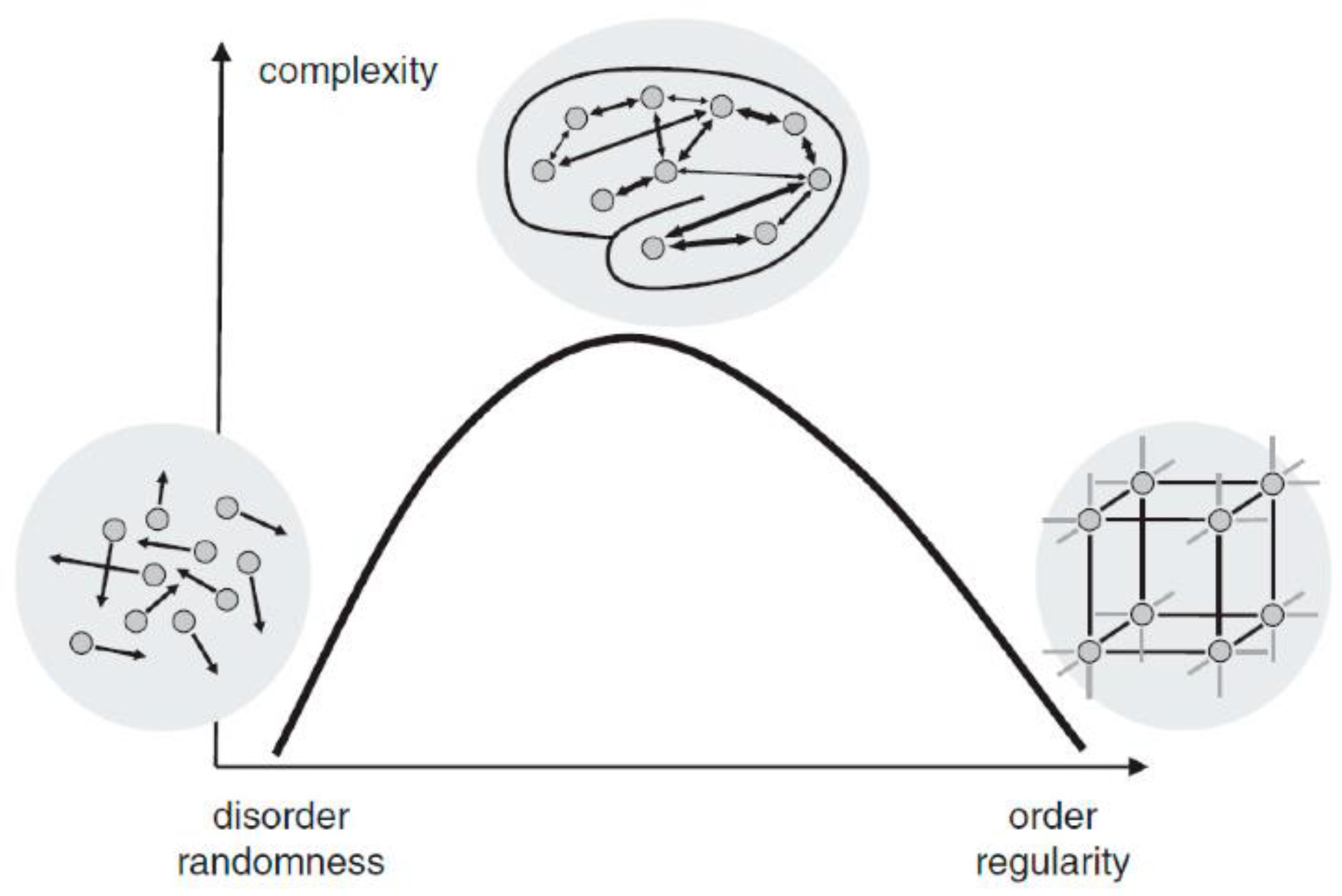
Figure 2.
The relation between the level of randomness and conventional entropy measure (a) and expected complexity (b). Reprinted from [1] with permission from ref. [4]. Copyright 2021 Elsevier.
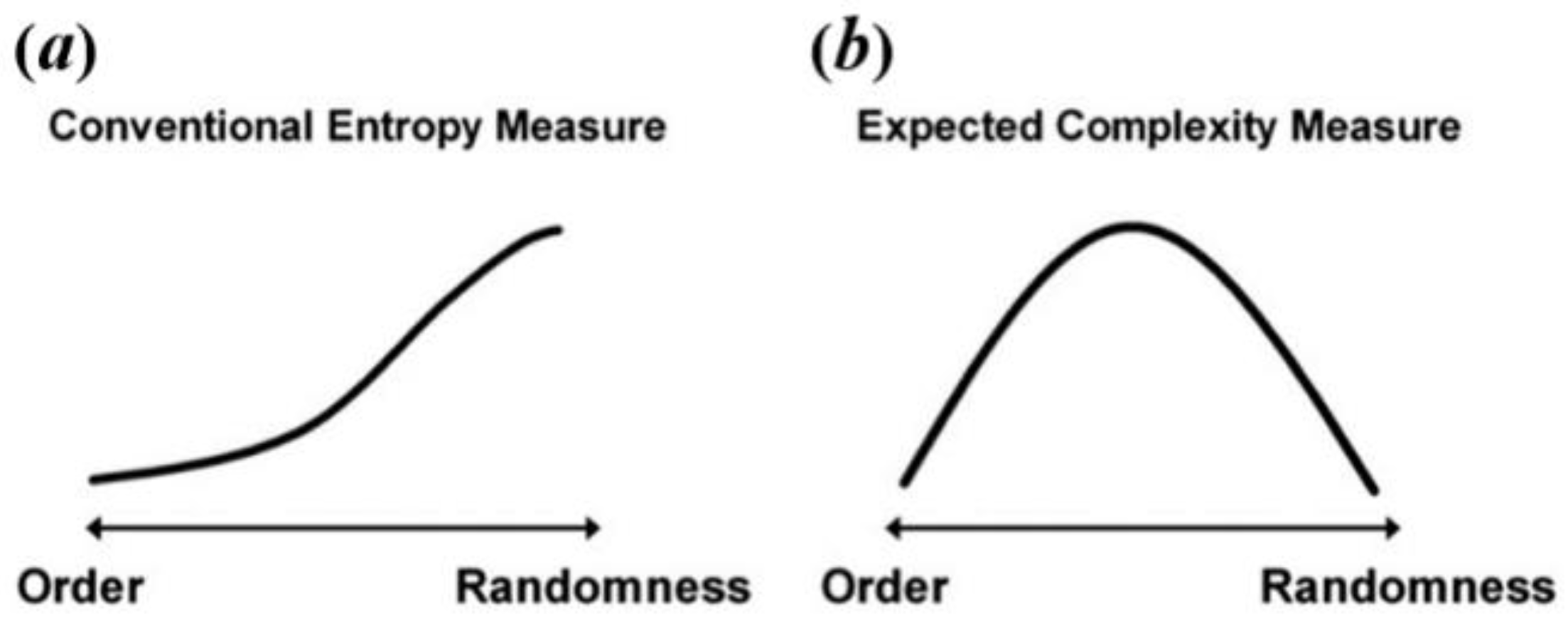
Figure 3.
(a) The values of interacting amplitudes of the master and individual KC spectra that are set along and axes (blue squares), respectively. KC spectra of the entire system (, black circles) and its component (, red circles) were calculated from the time series generated by a random generator (see previous subsection), (b) the same as in Figure 3b but with interacting amplitudes included in the set (blue squares). Reprinted with permission Copyright 2025 Universal Wiser.
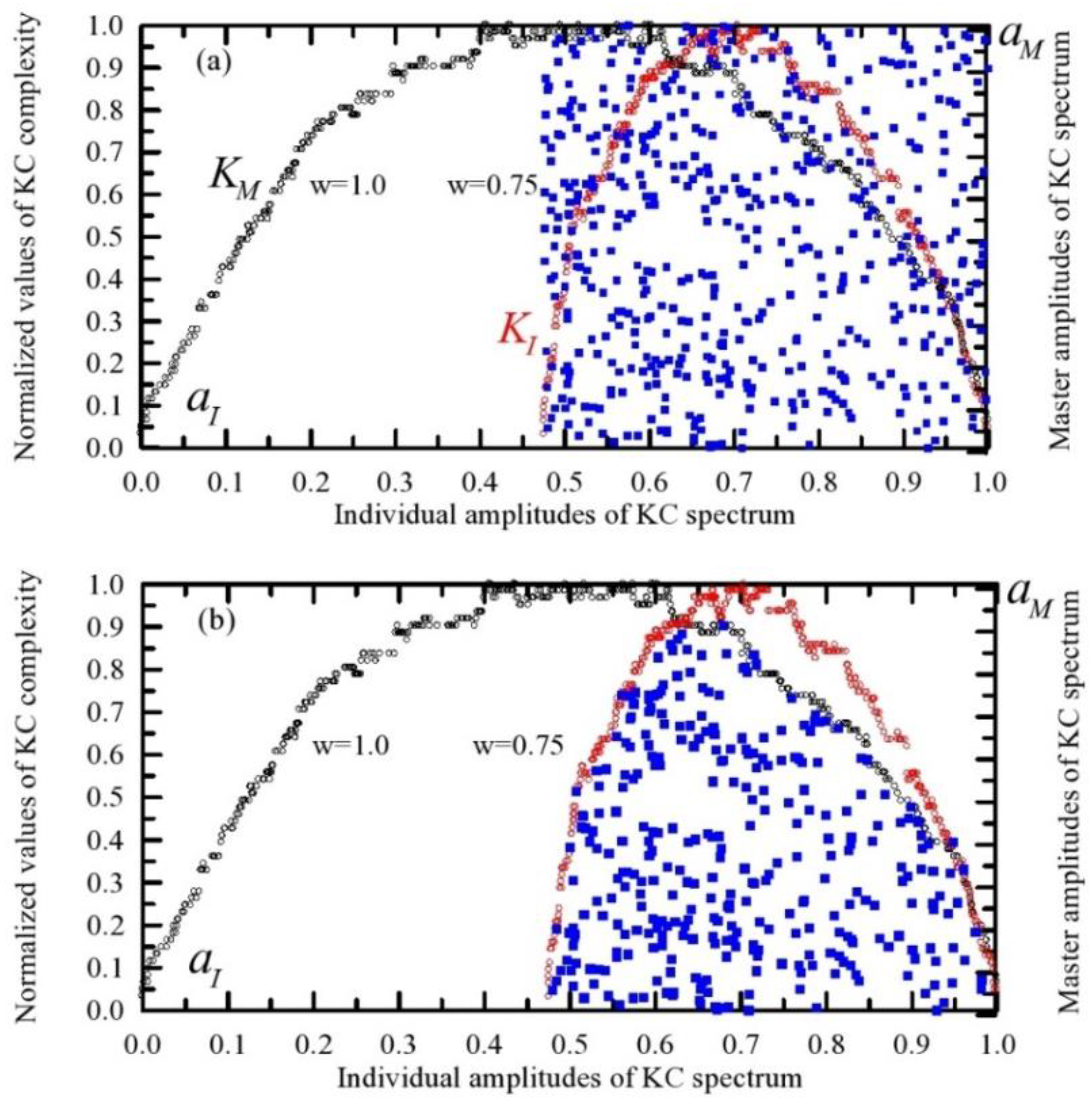
Figure 4.
Time series of (a) observed and (b) modeled precipitation in Sombor, Serbia (1982–2005). All values are normalized.
Figure 4.
Time series of (a) observed and (b) modeled precipitation in Sombor, Serbia (1982–2005). All values are normalized.
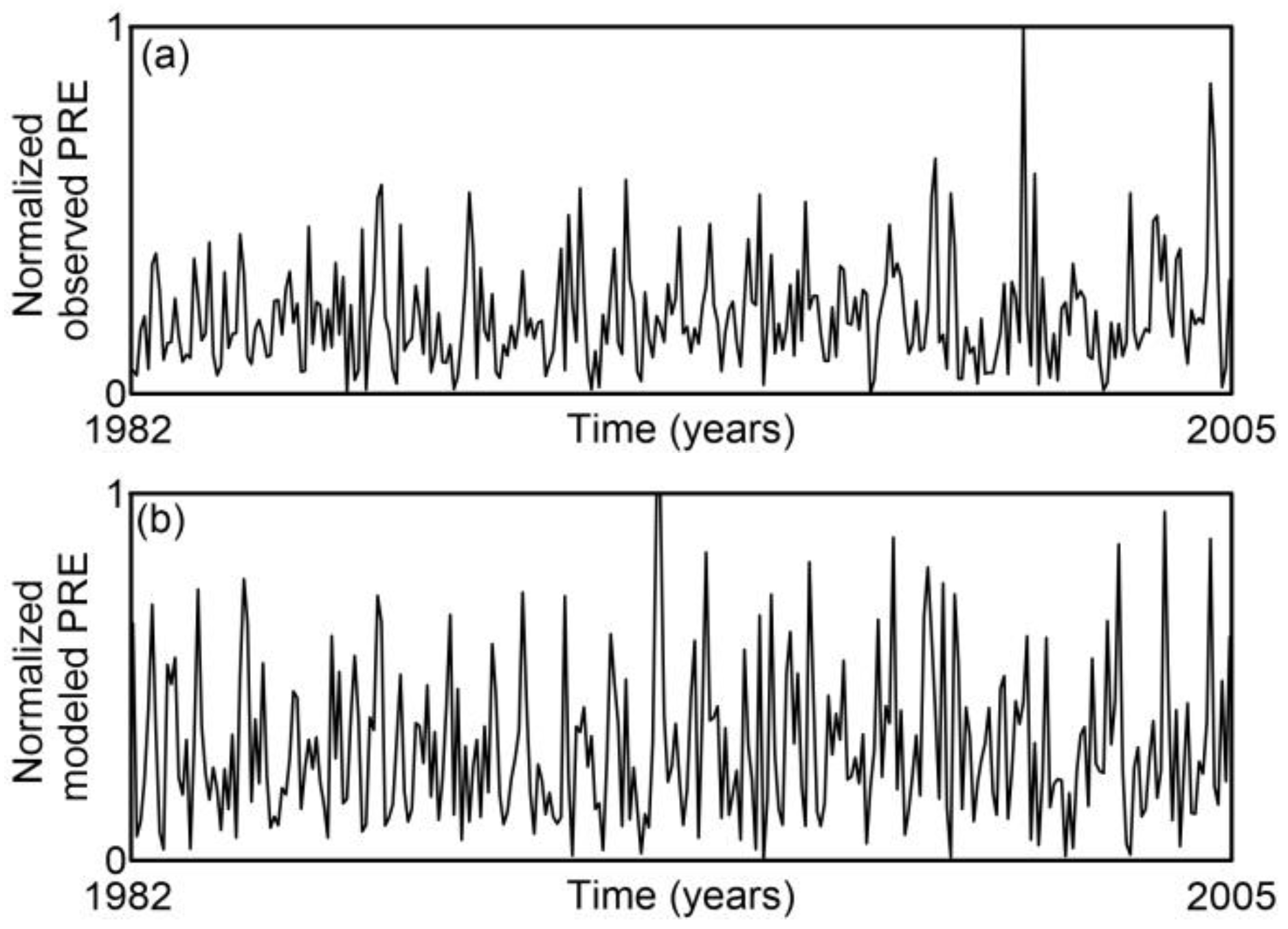
Figure 5.
Time series of average temperature (Tav), minimum temperature (Tmin), maximum temperature (Tmax), humidity (HUM), wind speed (WS), and global radiation (GR)observed in Sombor, Serbia (1982–2005). All values are normalized.
Figure 5.
Time series of average temperature (Tav), minimum temperature (Tmin), maximum temperature (Tmax), humidity (HUM), wind speed (WS), and global radiation (GR)observed in Sombor, Serbia (1982–2005). All values are normalized.
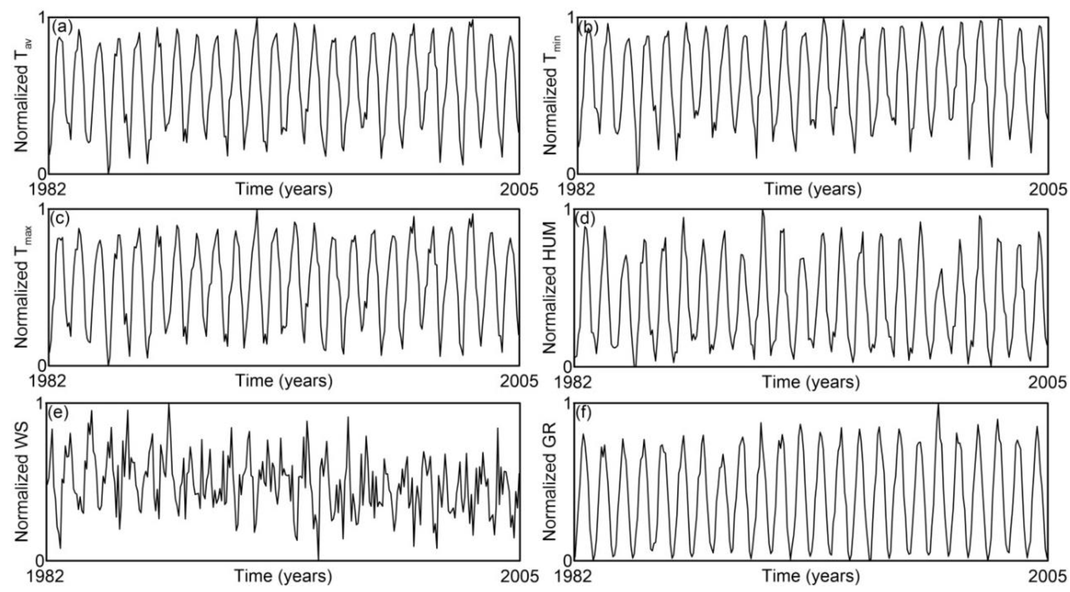
Figure 6.
Time series of average temperature (Tav), minimum temperature (Tmin), maximum temperature (Tmax), humidity (HUM), wind speed (WS), and global radiation (GR) in Sombor, Serbia (1982–2005), derived from simulation by the EBU-POM model. All values are normalized.
Figure 6.
Time series of average temperature (Tav), minimum temperature (Tmin), maximum temperature (Tmax), humidity (HUM), wind speed (WS), and global radiation (GR) in Sombor, Serbia (1982–2005), derived from simulation by the EBU-POM model. All values are normalized.
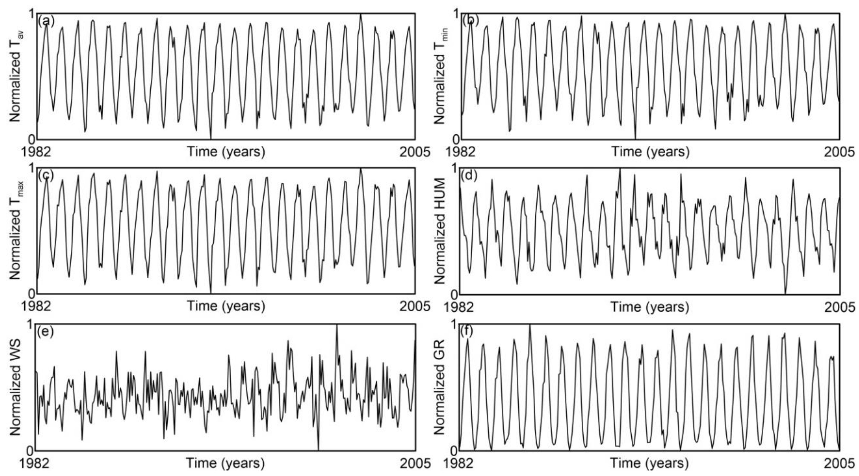
Figure 7.
The values of interacting amplitudes between the master and individual KC spectra for the observed data in Sombor, Serbia that are set along and axes (blue squares) included in the set, respectively. KC spectra of the entire system (KM) are represented by black circles, while KC spectra of its components (KI) are red circles.
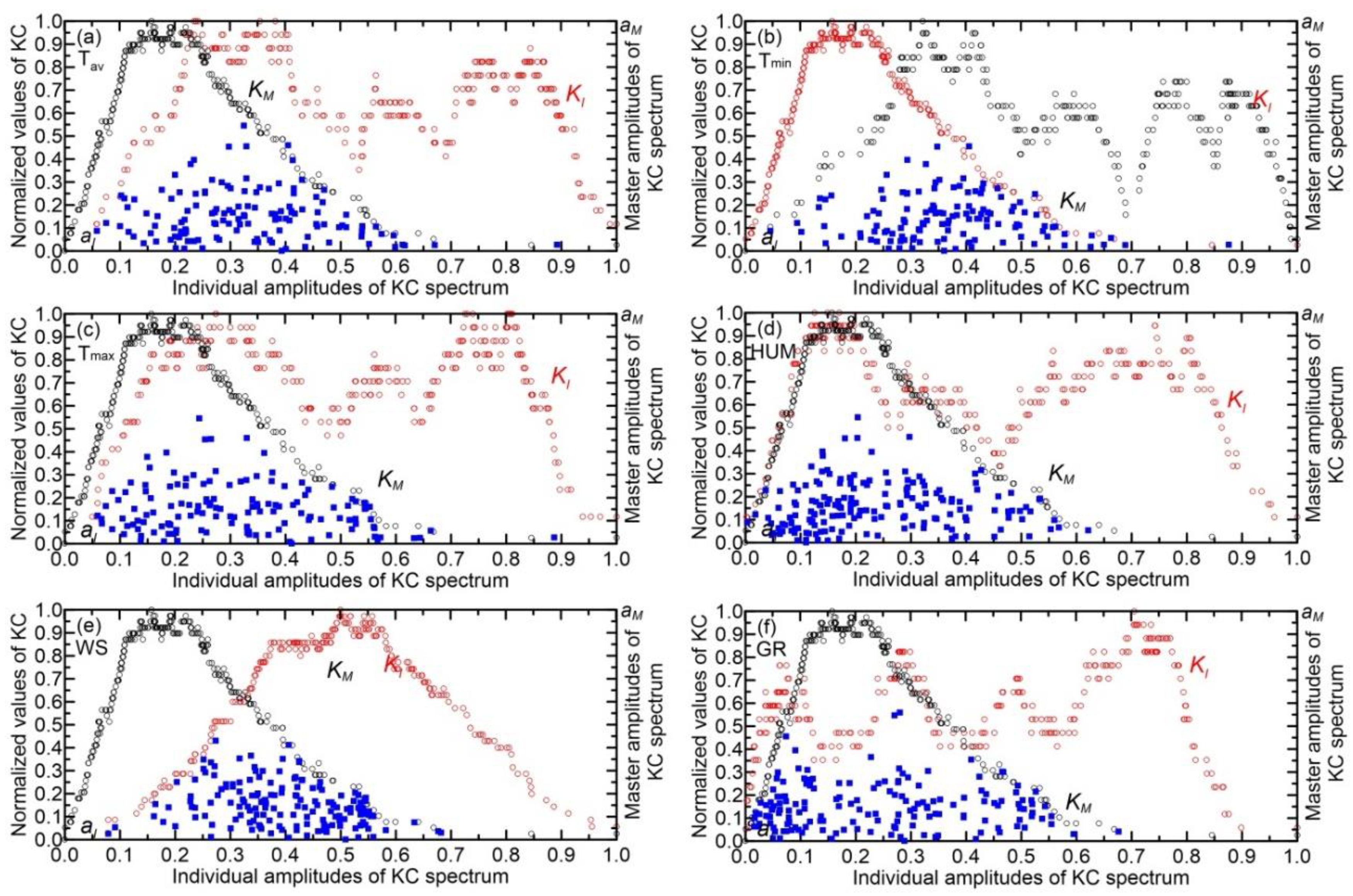
Figure 8.
Equivalent to Figure 7, but using EBU-POM output data.
Figure 8.
Equivalent to Figure 7, but using EBU-POM output data.
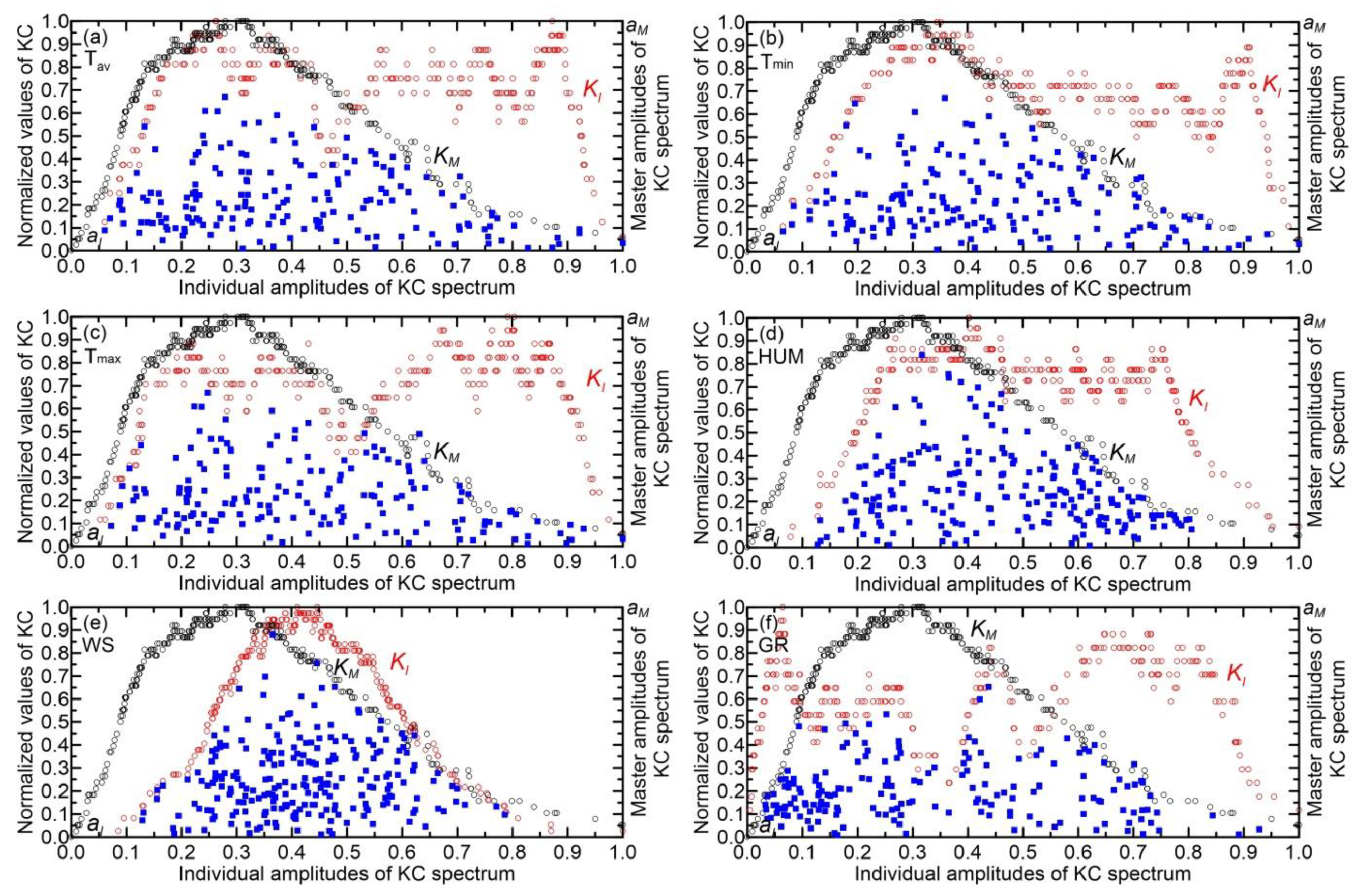
Figure 9.
Relative change in the overall complexity of precipitation (PRE) compared to complexity, considering individual components such as average temperature (Tav), minimum temperature (Tmin), maximum temperature (Tmax), humidity (HUM), wind speed (WS), and global radiation (GR).
Figure 9.
Relative change in the overall complexity of precipitation (PRE) compared to complexity, considering individual components such as average temperature (Tav), minimum temperature (Tmin), maximum temperature (Tmax), humidity (HUM), wind speed (WS), and global radiation (GR).
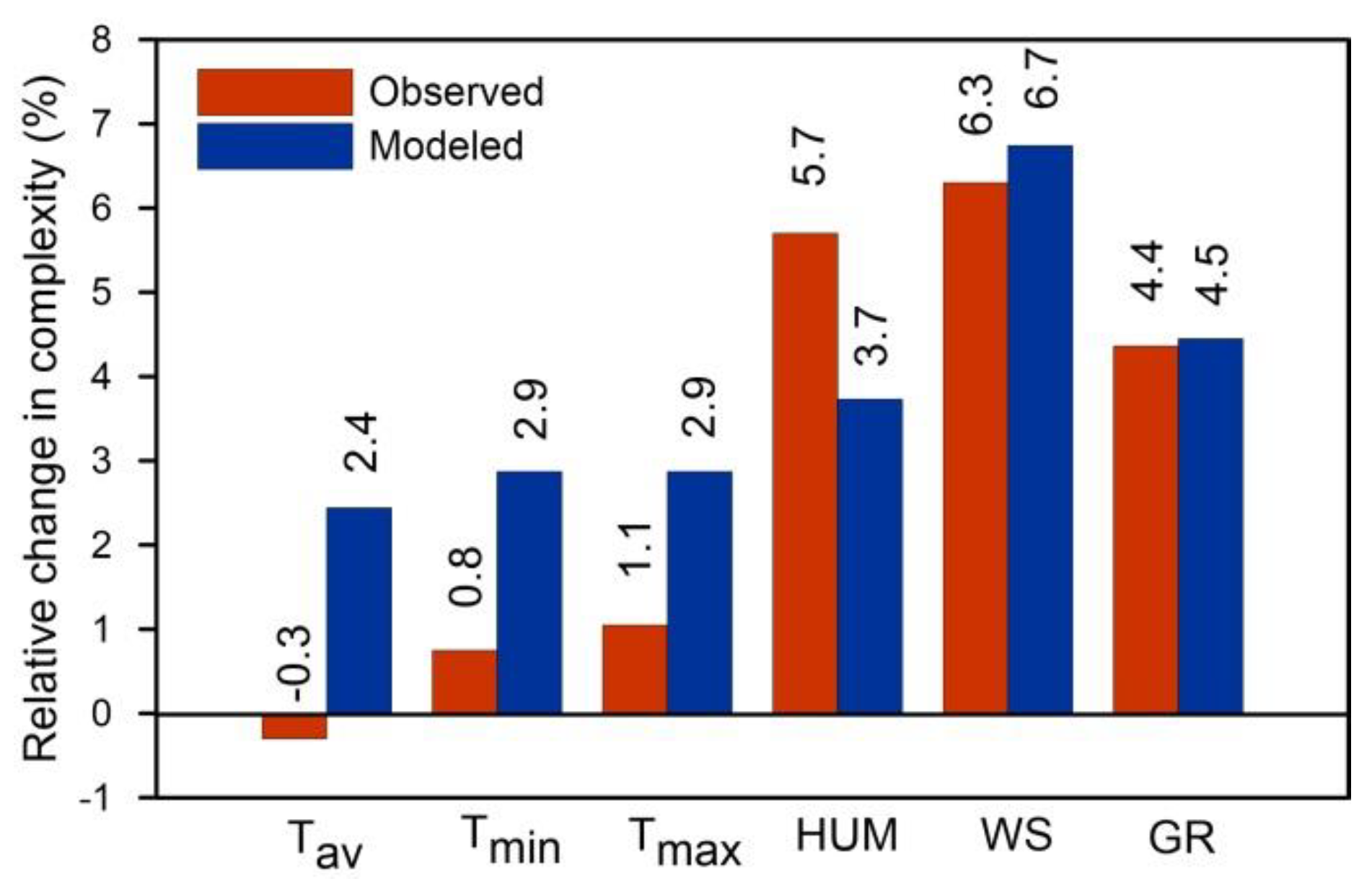

Table 1.
Maximum and minimum values in the time series prior to normalization.
| Variable | Modeled | Observed | ||
| Max | Min | Max | Min | |
| Precipitation (PRE) | 156.8 mm | 0.0 mm | 231.0 mm | 0.8 mm |
| Mean temperature (Tav) | 24.5 oC | -5.7 oC | 25.0 oC | -6.3 oC |
| Minimum temperature (Tmin) | 16.9 oC | -9.6 oC | 16.8 oC | -10.4 oC |
| Maximum temperature (Tmax) | 31.9 oC | -2.7 oC | 33.8 oC | -2.3 oC |
| Humidity (HUM) | 86.2% | 29.3% | 82.4% | 29.4 % |
| Wind speed (WS) | 3.8 ms-1 | 1.8 ms-1 | 2.7 ms-1 | 1.2 ms-1 |
| Global radiation (GR) | 316.9 Wm-2 | 29.3 Wm-2 | 325.2 Wm-2 | 34.2 Wm-2 |
Table 2.
Statistics with observed data for Sombor (Serbia). Gray highlighted numbers represent the maxima in each column.
Table 2.
Statistics with observed data for Sombor (Serbia). Gray highlighted numbers represent the maxima in each column.
|
Normalized individual amplitude |
Values of KC in overlapping area (OA) and (number of points in OA) | |||||
| Tav | Tmin | Tmax | HUM | WS | GR | |
| 0.0-0.1 | 0.756 (2) | 0.756 (2) | 0.817 (7) | 0.620 (27) | 0.295 (2) | 0.694 (45) |
| 0.1-0.2 | 0.704 (19) | 0.734 (8) | 0.614 (31) | 0.688 (61) | 0.795 (4) | 0.684 (26) |
| 0.2-0.3 | 0.646 (37) | 0.621 (29) | 0.722 (32) | 0.738 (31) | 0.725 (23) | 0.640 (30) |
| 0.3-0.4 | 0.687 (32) | 0.677 (38) | 0.698 (39) | 0.773 (28) | 0.749 (50) | 0.766 (21) |
| 0.4-0.5 | 0.722 (24) | 0.768 (32) | 0.698 (17) | 0.748 (17) | 0.692 (43) | 0.691 (21) |
| 0.5-0.6 | 0.627 (11) | 0.662 (11) | 0.673 (16) | 0.701 (9) | 0.710 (33) | 0.777 (13) |
| 0.6-0.7 | 0.179 (3) | 0.292 (5) | 0.256 (3) | 0.410 (1) | 0.325 (3) | 0.282 (1) |
| 0.7-0.8 | ||||||
| 0.8-0.9 | 0.179 (1) | 0.179 (1) | 0.179 (1) | |||
| 0.9-1.0 | ||||||
| Average (sum) | 0.665 (129) | 0.672 (126) | 0.674 (136) | 0.705 (174) | 0.709 (158) | 0.696 (157) |
Table 3.
Statistics with EBU-POM output data for Sombor (Serbia). Gray highlighted numbers represent the maxima in each row.
Table 3.
Statistics with EBU-POM output data for Sombor (Serbia). Gray highlighted numbers represent the maxima in each row.
|
Normalized individual amplitudes |
Values of KC in overlapping area (OA) and (number of points in OA) | |||||
| Tav | Tmin | Tmax | HUM | WS | GR | |
| 0.0-0.1 | 0.772 (6) | 0.693(3) | 0.772 (3) | 0.756 (31) | ||
| 0.1-0.2 | 0.734 (20) | 0.727 (19) | 0.741 (23) | 0.583 (12) | 0.546 (8) | 0.711 (37) |
| 0.2-0.3 | 0.745 (38) | 0.786 (29) | 0.758 (39) | 0.769 (35) | 0.774 (36) | 0.763 (31) |
| 0.3-0.4 | 0.740 (34) | 0.737 (34) | 0.762 (24) | 0.647 (37) | 0.721 (60) | 0.908 (10) |
| 0.4-0.5 | 0.778 (22) | 0.742 (30) | 0.788 (24) | 0.721 (33) | 0.723 (68) | 0.744 (23) |
| 0.5-0.6 | 0.757 (23) | 0.728 (23) | 0.751 (20) | 0.811 (35) | 0.813 (40) | 0.687 (11) |
| 0.6-0.7 | 0.679 (10) | 0.719 (13) | 0.726 (12) | 0.754 (39) | 0.778 (20) | 0.713 (19) |
| 0.7-0.8 | 0.613 (14) | 0.668 (16) | 0.616 (15) | 0.668 (18) | 0.737 (3) | 0.626 (13) |
| 0.8-0.9 | 0.237 (5) | 0.417 (6) | 0.312 (7) | 0.579 (2) | 0.303 (2) | |
| 0.9-1.0 | 0.377 (3) | 0.281 (3) | 0.322 (4) | 0.184 (1) | ||
| Average (sum) | 0.714 (175) | 0.717 (176) | 0.717(171) | 0.723 (211) | 0.744 (235) | 0.728 (178) |
Disclaimer/Publisher’s Note: The statements, opinions and data contained in all publications are solely those of the individual author(s) and contributor(s) and not of MDPI and/or the editor(s). MDPI and/or the editor(s) disclaim responsibility for any injury to people or property resulting from any ideas, methods, instructions or products referred to in the content. |
© 2025 by the authors. Licensee MDPI, Basel, Switzerland. This article is an open access article distributed under the terms and conditions of the Creative Commons Attribution (CC BY) license (http://creativecommons.org/licenses/by/4.0/).
Copyright: This open access article is published under a Creative Commons CC BY 4.0 license, which permit the free download, distribution, and reuse, provided that the author and preprint are cited in any reuse.


