Submitted:
07 June 2025
Posted:
09 June 2025
You are already at the latest version
Abstract
When there are several different types of heat-storage ceramic bricks that can be arranged in the fix-bed heat regenerators of a regenerative combustion system, one must find an optimal arrangement of these bricks, of possibly different types, in the fix-bed heat regenerators of a regenerative combustion system. It seems impractical to evaluate the efficiency of each of all the possible arrangements of heat-storage ceramic bricks, in the fix-bed heat regenerators of a rege-nerative combustion system, by 3-dimensional CFD (Computational Fluid Dynamics) simulations on Ansys Fluent. In this article, we present an efficient tree search method to tackle this optimization problem.
Keywords:
regenerative combustion
; heat transfer
; optimization
; simulation
; Monte Carlo method
; tree search
1. Introduction
In this article, we will propose a method for solving an optimization problem on the arrangements of heat-storage ceramic bricks (checkers) in a heat regenerator system.
Usually two fixed-bed heat regenerators are utilized in pairs with a central furnace to form a regenerative combustion system. See Figure 1. In each heat regenerator, checkers are arranged. The regenerative combustion system operates periodically with a two-phase cycle. The checkers arranged in the heat regenerators, on both ends of a regenerative combustion system, are used to absorb heat from the high temperature exhaust gas expelled from the central furnace.
In Phase 1, the cool fresh air flows into the left heat regenerator and is preheated by the checkers arranged there. (The checkers arranged in the left heat regenerator are designed to absorb periodically heat from the high temperature exhaust gas expelled from the central furnace in Phase 2.) The preheated fresh air then flows into the central furnace for combustion with Natural Gas. After combustion with Natural Gas, the high temperature exhaust gas, expelled from the central furnace, then flows into the right heat regenerator and heats up the checkers arranged there. Then Phase 2 starts at the Phase Switch point of time. In Phase 2, the above process is reversed. The cool fresh air flows into the right heat regenerator and is preheated by the checkers arranged there, which already absorbed heat from the high temperature exhaust gas expelled from the central furnace during Phase 1. Then the preheated fresh air flows into the central furnace for combustion with Natural Gas. Finally, the high temperature exhaust gas, expelled from the central furnace, flows into the left heat regenerator and heats up the checkers arranged there. Then Phase 1 starts again at the Phase Switch point of time. A new cycle of operations follows.
Usually there are several different types of heat-storage ceramic bricks that can be arranged in a heat regenerator. So one must find an optimal arrangement of these checkers, of possibly several different types, in a heat regenerator to reach the best performance of the regenerative combustion system with this heat regenerator. Naturally, the objective function for this optimization problem is the long-term Waste Heat Recovery Ratio defined for each arrangement of selected heat-storage ceramic bricks (of possibly different types) in this heat regenerator.
However, the number of possible arrangements of checkers in a heat regenerator could be very huge. Thus finding the optimal arrangement of checkers, of possibly different types, in a heat regenerator could be difficult. In fact, when there are different types of checkers that can be selected for each of positions in a fixed-bed heat regenerator, the total number of possible arrangements of checkers at positions is
Thus, when 5 different types of checkers are available for each of 14 positions in a heat regenerator, the total number of possible arrangements of checkers, of possibly different types, is
This means that one must evaluate more than 6 billion arrangements to reach an optimal arrangement of checkers at 14 positions in a heat regenerator. To tackle this optimization problem, one must find a effective method for deciding the optimal (most efficient) arrangements of checkers among the huge number of possible arrangements of checkers, of possibly different types, at positions in a fixed-bed heat regenerator.
Over the past few years, the Artificial Intelligence (AI), based on combination of “Deep Learning” with MCTS, has proved to be very successful in creating computer player for the incredibly complicated board game Go. Motivated by this great progress in AI, we propose, in this article, a simple stochastic tree search method to find the most efficient arrangement of checkers in a heat regenerator.
Though the total number
depends exponentially on the number of positions for checkers in a heat regenerator, our stochastic tree search method usually exhibits only complexity of polynomial growth on the number of positions for checkers in a heat regenerator.
To speed up the search process for the most efficient arrangements of checkers, we use a simplified system of 1-dimensional partial differential equations to evaluate the long-term Waste Heat Recovery Ratio of each node (arrangement of checkers) considered in our search tree. We demonstrate this search method to find the most efficient arrangements of checkers when the number of positions for checkers in a heat regenerator is 6. Empirical results reveal that our search method is highly efficient for finding the optimal arrangements of checkers in a heat regenerator.
2. Materials and Methods
The “Monte-Carlo Method” was proposed in 1949, [1], to calculate the area of a region, based on Random Sampling, to solve problems in statistical physics. According to the mathematical principle “Law of Large Numbers”, [2,3,4], one should be able to speculate almost correctly the genuine area of a region when the sampling number is large enough. By the way, other probabilistic methods “Stochastic Integrals”, [5,6], based on the Central Limit Theorem, were applied to mathematical finance, [7], in those decades.
2.1. Tree Search by the Monte-Carlo Method
In 1987, B. Abramson applied the “Monte-Carlo Method” to certain “Two-Player Games”: tic-tac-toe, Othello and Chess, [8]. B. Abramson proposed the “Expected-Outcome model”, based on the statistical data of “random game playouts to the end”, as the basis of strategies for a game player. B. Brügmann considered the applications of the “Monte-Carlo Method” to the board game “Go” in 1993, but not seriously, [9]. In 2006, inspired by many predecessors, R. Coulom considered seriously the applications of the “Monte-Carlo Method” to the search tree for the board game “Go”, [10]. See also [11] for the work by Kocsis and Szepesvári. The decision-making algorithm proposed in [10] was considered as “Monte-Carlo Tree Search (MCTS)” by R. Coulom. More modifications and improvements, [12,13,14,15,16,17,18], are made for MCTS after the important contributions by Kocsis and Szepesvári, [11] and by Coulom, [10]. The MCTS algorithm was also applied to certain games, [19,20,21,22,23]. By combining MCTS with Reinforcement Learning based on CNN (Convolutional Neural Networks), the computer Go player AlphaGo, developed by Google DeepMind, defeated Lee, Sedol, one of the most brilliant Go players, in a five game Go match in 2016. See [24,25]. The following three pictures are taken from [26], which can be found on the website of Rémi Coulom.
Figure 2.
List of Game Complexity. Taken from [26].
Figure 2.
List of Game Complexity. Taken from [26].
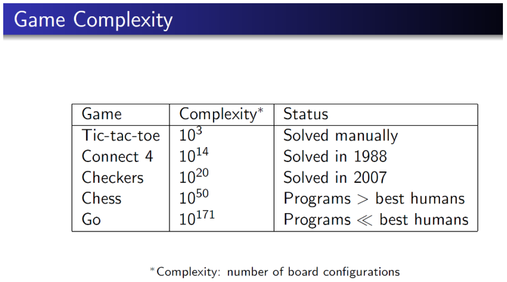
Figure 3.
Principle of Monte-Carlo Evaluation. Taken from [26].
Figure 3.
Principle of Monte-Carlo Evaluation. Taken from [26].

Figure 4.
Monte-Carlo Tree Search. Taken from [26].
Figure 4.
Monte-Carlo Tree Search. Taken from [26].

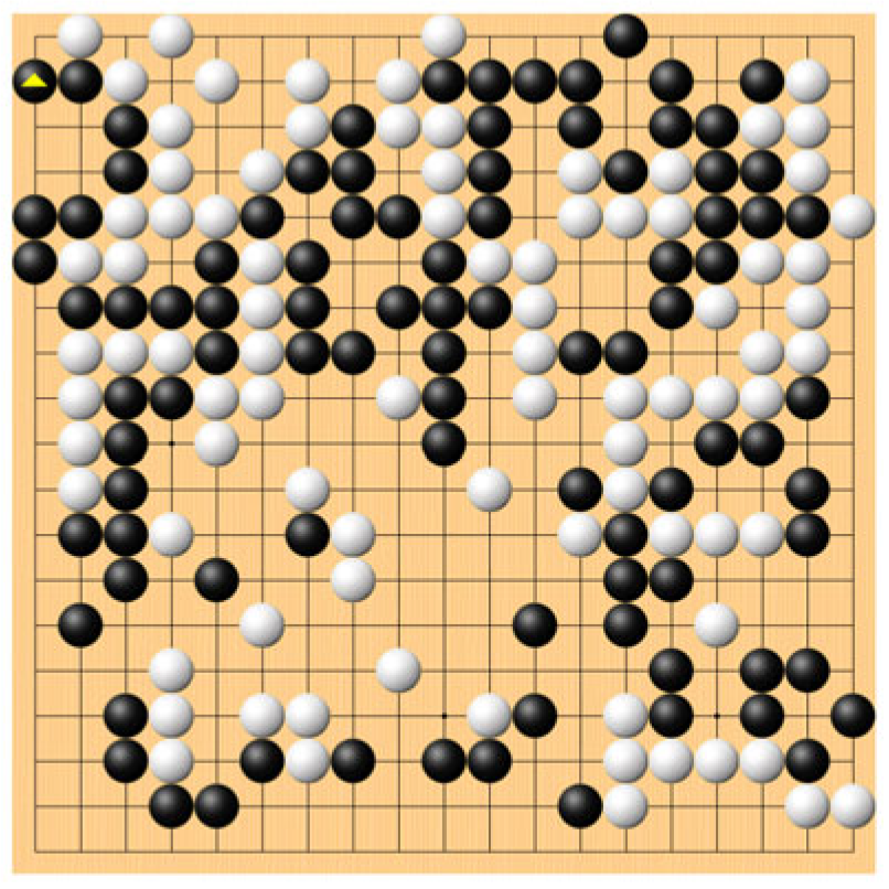
Figure 5.
The board game Go.
In 2017, Google DeepMind added a new ingredient “Dirichlet noise” to AlphaGo Zero to encourage further exploration by MCTS, which could be omitted by the earlier versions of AlphaGo because of low prior probabilities. This deepened the MCTS reinforcement learning of AlphaGo Zero. AlphaGo Zero is considered as a genuine AI because AlphaGo Zero is able to explore the board game Go by MCTS without human knowledge (experience), [27]. Applications of Artificial Intelligence with MCTS to other games were developed in [28,29,30,31]. Artificial Intelligence with MCTS was also applied to chemical syntheses of organic compounds, [32]. Application of MCTS to floor plans was considered in [33]. More applications of MCTS are still explored, [34,35]. For a recent review on MCTS, see [36].
2.2. Our Simple Tree Search Method
Motivated by the principles of MCTS, we will introduce a simple Tree Search method to find the optimal (most efficient) arrangements of heat-storage ceramic bricks (checkers) in a heat regenerator, when there are different types of checkers that can be selected for each of positions in a fixed-bed heat regenerator. Our search method can be performed easily on an ordinary computer, while a super computer is usually necessary for AI with MCTS.
We begin with the notion of a “Partition” of the set
of positions, to be placed by checkers, in a fixed-bed heat regenerator. A Partition of is a subset of such that the largest integer must be included in .
Example 1. For the set , and are Partitions of .
Assume that
is a Partition of . Using the positive integers in , we may create the following decomposition
for , in which
Example 2. For the Partition of the set , we have the following decomposition
with and .
For the Partition
with
of the , we will conveniently say that each is an “Interval Component” of with respect to , because each contains certain consecutive positive integers taken from . This phenomenon is clear from the example (Example 2) shown above.
We have the following simple facts about the decomposition (2) of .
Fact A. The endpoints of the Interval Components in (2) simply constitute the Partition set of .
Fact B. The Interval Components of the decomposition (2) of , with respect to the Partition , are disjoint.
Fact C. Elements of the Interval Components of the decomposition (2) of are linearly ordered.
There is a Partial Ordering on the collection of all Partitions of . For Partitions and of , we say that is finer than if and only if
We say that is strictly finer than if and only if
We will use the notation
to indicate the condition that is strictly finer than .
Example 3. For the Partitions and of , we have .
Now we discuss the notion of “qualified arrangements with respect to a Partition”. Assume that is a Partition of as shown in (1). We say that an arrangement of checkers on is a “qualified arrangement with respect to the Partition ” if and only if the following condition (4) is satisfied.
Definition. We say that an arrangement of checkers on is a “qualified arrangement with respect to the Partition ” if the following condition is satisfied.
For each Interval Component of in the decomposition (2) with respect to the Partition ,
Let denote the class of all “qualified arrangements with respect to the Partition ”. Let denote the norm (the total number of qualified arrangements with respect to ) of . Then we have
in which is the norm (number of elements) of , as shown in (1).
Example 4. For the Partition of , the total number of “qualified arrangements with respect to the Partition ” is
For the Partition , the total number of “qualified arrangements with respect to the Partition ” is
However, the number of all possible arrangements of checkers on is .
For Partitions and of , we have the following important
Fact D. For Partitions and of satisfying , we have
Thus any “qualified arrangement of checkers with respect to the Partition ” is naturally a “qualified arrangement of checkers with respect to the Partition ”. Besides, the class of arrangements is strictly larger than the class of arrangements.
To initialize a search tree for the optimal (most efficient) arrangements of checkers in a heat regenerator, when different types of checkers are available for selection at each of positions in the heat regenerator, we must choose a strictly increasing sequence
of Partitions of . Let denote the class of all “qualified arrangements with respect to the Partition ”. Then, according to Fact D, the sequence of classes
of arrangements corresponding to the strictly increasing sequence of Partitions, is naturally strictly increasing.
In our tree search, each arrangement of checkers on will be considered as a “node” in the search tree. At the initial stage , we evaluate the efficiency of each of the arrangements in (“qualified arrangements with respect to the Partition ”) by numerical Simulation. Then we select the top arrangements in as the “mother (root) nodes” in . These selected “mother (root) nodes” will be used to create “child nodes” (qualified arrangements with respect to the Partition ) in . This process is the Expansion operator of our algorithm. Then we evaluate the efficiency of each of the child nodes, created by the Expansion operator, in by numerical Simulation. See Figure 6 for the phases of our tree search.
In the Expansion phase of Figure 6, The “mother (root) nodes” selected in will be used to create “child nodes” in .
2.3. The Expansion Operators
We will discuss two Expansion operators, “Gradient Expansion operator” and “Mutation Expansion operator”, for our tree search method.
We consider the following typical case. Assume that and are Partitions of satisfying
Then, by Fact D, we have
Let
be the decomposition of into a union of Interval Components with respect to the Partition . Assume that . Since , we note that, for each Interval Component , only checkers of the same type are placed on by the arrangement . We assume that, on the Interval Component , the checkers arranged by are all of the type
Assume that is a “qualified arrangement with respect to the Partition ”. Assume that, on the Interval Component , the checkers arranged by are all of the type
We say that the arrangement of checkers is a “child-node” of in , by the “Gradient Expansion operator”, if the following GE Condition is satisfied.
GE(Gradient Expansion) Condition. There is a sequence of positive integers taken from , satisfying
such that
For each , we have
for the arrangements and of checkers on the pair of adjacent Interval components and . Besides, outside these pairs of adjacent Interval components, , we have
Example 5. For the Partitions and of , we have
These are the decompositions of into unions of Interval Components respectively with respect to the Partitions and . Assume that we have two different types of checkers and . Then
is a qualified arrangement of checkers with respect to the Partition . When is considered as a qualified arrangement with respect to the Partition , it has the following child-nodes
by the “Gradient Expansion operator”.
This “Gradient Expansion operator” is motivated by the usual Gradient Descent method adopted in Machine Learning. See, for example, [37]. Search through the simple Gradient Descent method usually converges slowly. (To expedite the training process of AI, Stochastic Gradient Descent was introduced. See [37].)
Now we discuss the “Mutation Expansion operator” under the assumptions (9) to (12). We say that the arrangement of checkers is a “child-node” of in , by the “Mutation Expansion operator”, if the following ME Condition is satisfied.
ME(Mutation Expansion) Condition. There is a sequence of positive integers taken from , satisfying
such that
For each , we have
for the arrangements and of checkers on the pair of adjacent Interval components and . Besides, outside these pairs of adjacent Interval components, , we have
Example 6. For the Partitions and of , we have the following decompositions
of into unions of Interval Components respectively with respect to the Partitions and . Assume that we have two different types of checkers and . Then
is a qualified arrangement of checkers with respect to the Partition . When is considered as a qualified arrangement with respect to the Partition , it has the following child-nodes
by the “Mutation Expansion operator”.
This “Mutation Expansion operator” is motivated by the Differential Evolution method. See, for example, [38,39,40,41]. Search through this “Mutation Expansion operator” usually lead to rapid convergence. Thus we may use “tree search through the Mutation Expansion operator” to help us to find a satisfactory strictly increasing sequence
of Partitions of . Then we may use this proper strictly increasing sequence of Partitions of to execute a delicate “tree search through the Gradient Expansion operator”, which usually converges slowly.
2.4. The Numerical Simulation Methods
To speed up the evaluation process for an arrangement of checkers in a fixed-bed heat regenerator, our numerical simulations are based on certain 1-dimensional partial differential equations as in [42,43,44]. These 1-dimensional partial differential equations were developed in [45,46] based on the theories of W. Nusselt. Empirical evidence shows that, in the long term, simulation results of the Inlet temperature and the Outlet temperature, by the 1-dimensional partial differential equations, are consistent with that by CFD (Computational Fluid Dynamics) on Ansys Fluent.
Let us consider the two-phase cycle of a fixed-bed heat regenerator, which is placed on the right end of a regenerative combustion system, as shown in Figure 7. In Phase 1, the high temperature exhaust gas, from the central furnace, flows into the right heat regenerator and heats up the checkers arranged there. Then Phase 2 starts at the Phase Switch point of time. In Phase 2, the above process is reversed. The cool fresh air flows into the right heat regenerator and is preheated by the checkers arranged there, which already absorbed heat from the high temperature exhaust gas expelled from the central furnace during Phase 1. Then the preheated fresh air flows into the central furnace for combustion with Natural Gas.
Let denote the switch time of the operation cycle of the fixed-bed heat regenerator shown above. Thus
is the period of the operation cycle. When , Phase 1 operates. When , Phase 2 operates. To evaluate the efficiency of an arrangement of checkers on a fixed-bed heat regenerator, this operation cycle must be performed periodically until we reach approximately at a steady state. We assume that the fixed-bed heat regenerator is located on the interval of the -axis. See Figure 7.
We use the subscript ar to indicate functions related to the fresh air flow. We use the subscript ex to indicate functions related to the exhaust gas flow. We use the subscript s to indicate functions related to the checkers (solid porous medium). Let be a nonnegative integer. When
we have the following 1-dimensional partial differential equations:
and
satisfying the following boundary conditions
When , we have the following 1-dimensional partial differential equations:
and
satisfying the following boundary conditions
Here (m/s) is the superficial flow velocity of the gas/air. (kg/m3) and (kg/m3) are respectively the densities of the gas/air and the solid porous medium (checkers). (J/kgK) and (J/kgK) are respectively the specific heat capacities of the gas/air and the solid porous medium (checkers). (W/mK) and (W/mK) are respectively the thermal conductivities of the gas/air and the solid porous medium (checkers). (K) and (K) are respectively the temperatures of the gas/air and the solid porous medium (checkers). is the void fraction (porosity) of the solid porous medium (checkers). (m2) is the specific surface area of the porous ceramic medium (checkers) exposed to gas/air per unit volume. (w/m2K) is the heat transfer coefficient of the solid porous medium (checkers). is the heat dissipation through the external surface of a fixed-bed heat regenerator. We assume that .
We have the following relation for the Nusselt number of the fluid (gas/air) flow:
in which is the characteristic length. Let and denote respectively the Reynolds number and the Prandtl number of the fluid (gas/air) flow. We will use the following classic relation
of Sieder and Tate to calculate the Nusselt number. Here and are respectively the viscosity of fluid at the mean bulk temperature and the viscosity of fluid at the wall. See page 583 of [47]. Note that
when is not large. Thus, when performing numerical simulations, we will use the simplified formula
Let (kg/s) and (kg/s) be respectively the mass flow rates of the exhaust gas flow and of the fresh air flow. Let (J/kgK) and (J/kgK) be the specific heat capacities of the fresh air respectively at the Inlet of fresh air (into the right heat regenerator) and at the Outlet of fresh air (into the central furnace). Let (K) and (K) be the temperatures of the fresh air respectively at the Inlet of fresh air (into the right heat regenerator) and at the Outlet of fresh air (into the central furnace). Let (J/kgK) be the specific heat capacity of the exhaust gas flow at the Inlet of exhaust gas (into the right heat regenerator). Let (K) be the temperature of the exhaust gas flow at the Inlet of exhaust gas (into the right heat regenerator).
We define the Waste Heat Recovery Ratio (%) of an arrangement of checkers in a fixed-bed heat regenerator as follows:
We use the long term Waste Heat Recovery Ratio to evaluate the efficiency of an arrangement of checkers in a fixed-bed heat regenerator.
To expedite the process of simulations, we use the following polynomials in our simulations.
These polynomials are derived based on the data provided in the Appendices of [48] at atmospheric pressure. For the densities of the air/gas, we use the following polynomial
in our simulations. This polynomial is derived based on the data for air provided in the Appendices of [48] at atmospheric pressure.
3. Results
Before starting our optimization process by tree search, we must test the validity of our 1-dimensional partial differential equations, though similar 1-dimensional modeling had been developed before in [42,43,44,45,46]. We test our 1-dimensional modeling for two types of checkers: Cordierite and Mullite with material parameters shown in Table 1. We consider the following arrangement of checkers
at 6 positions in a fixed-bed heat regenerator. We assume that the temperature of exhaust gas, expelled from the central furnace, is 900℃ (1173.15K). We assume that the temperature of fresh air, at the Inlet, is 40℃ (313.15K). We assume that the time of Phase Switch is 30s. We assume that the superficial flow velocity of the exhaust gas is . We assume that the superficial flow velocity of the fresh air is .
The comparison of our 1-D simulations with the 3-D CFD simulations on Ansys Fluent for the arrangement of checkers
at 6 positions, in a fixed-bed heat regenerator, is shown in Figure 8.
In Figure 8, the Inlet temperature of exhaust gas (expelled from the central furnace) and the Outlet temperature of fresh air (into the central furnace), based on our 1-D simulations using C++, is shown in black color. In Figure 8, the Inlet temperature of exhaust gas (expelled from the central furnace) and the Outlet temperature of fresh air (into the central furnace), based on 3-D CFD simulations on Ansys Fluent, is shown in red color.
In Figure 8, the Outlet temperature of exhaust gas (expelled from the right heat regenerator) and the Inlet temperature of fresh air (into the right heat regenerator), based on our 1-D simulations using C++, is shown in blue color. In Figure 8, the Outlet temperature of exhaust gas (expelled from the right heat regenerator) and the Inlet temperature of fresh air (into the right heat regenerator), based on 3-D CFD simulations on Ansys Fluent, is shown in green color.
It can be observed that, in the long term, our numerical simulation results, based on the 1-dimensional partial differential equations, are consistent with the simulation results based on CFD (Computational Fluid Dynamics) on Ansys Fluent. See Figure 8.
Now we apply our simple tree search method with Mutation Expansion operator to solve the optimization problem for 3 types of checkers to be arranged at 6 positions in a fixed bed regenerator. The material parameters of these 3 types, A, B and C, of checkers are shown in Table 2. The operating parameters for a regenerative combustion system with two fixed-bed heat regenerators are shown in Table 3.
Thus we have . We choose the strictly increasing sequence
of Partitions of . Thus we have the following decomposition
of into a union of Interval Components
with respect to the Partition .
We select the top 15 arrangements in as the “mother (root) nodes” in to create “child nodes” (qualified arrangements with respect to the Partition ) in .
For a complete evaluation process for the total
possible arrangements of checkers, based on 1-D simulations, it takes 63 hours to finish this evaluation process. The top 3 arrangements are shown in Table 4.
For the optimization process by our simple tree search method, it takes only 6 hours to evaluate
possible arrangements of checkers, based on 1-D simulations. The top 3 arrangements, found by this simple tree search method, are shown in Table 5.
Thus empirical evidence shows that our tree search method is helpful and efficient. An algorithm based on our simple tree search method, with the Mutation Expansion operator, is shown in Figure 9.
4. Discussion
In this article, we propose a tree search method for finding the optimal arrangements of heat-storage ceramic bricks (checkers) in a heat regenerator. Empirical evidence shows that this simple tree search method is efficient and helpful.
This tree search method is motivated by the Monte-Carlo Tree Search (MCTS) algorithm used in Artificial Intelligence, combined with “Deep Learning”, to create computer players for the incredibly complicated board game Go. The combination of “Deep Learning” with MCTS has proved to be very successful in creating powerful computer players for the incredibly complicated board game Go.
The principles and ideas for MCTS are partly adopted and developed in this research. However, there is key difference between these problems. The mathematics behind the incredibly complicated board game Go is still not properly understood by humans. But for the optimization problem of arrangements of heat-storage ceramic bricks (checkers) in a heat regenerator, we do understand that the performance of all the arrangements of checkers is governed by Physics Laws. This might explain why our simple stochastic tree search method seems to exhibit high efficiency.
5. Conclusions
In this article, we propose a tree search method for finding the optimal arrangements of heat-storage ceramic bricks (checkers) in a heat regenerator. Empirical evidence shows that this simple tree search method is efficient and helpful.
Author Contributions
Conceptualization, T.-J.C., Y.-J.H. and C.-S. W.; Investigation, T.-J.C. and S.-C. C.; Methodology, T.-J.C. and Y.-J.H.; Software, T.-J.C. and S.-C. C.; Validation, T.-J.C., S.-C. C.; Writing—original draft, T.-J.C. and Y.-J.H. All authors have read and agreed to the published version of the manuscript.
Funding
This research was partly supported by the National Science and Technology Council of Taiwan Government, grant NSC 112-2115-M-006 -007 -.
Data Availability Statement
Not applicable.
Conflicts of Interest
The authors declare no conflict of interest.
References
- N. Metropolis, N.; Ulam, S. The Monte Carlo Method. Journal of the American Statistical Association. 1949, 44, 335–341. [Google Scholar] [CrossRef] [PubMed]
- Terrell, G. Mathematical Statistics: A Unified Introduction; Springer-Verlag, New-York, Inc., 1999.
- DeGroot, M; Schervish, M. Probability and Statistics; Pearson Education, Inc., 2012.
- Roe, B. Probability and Statistics in the Physical Sciences; Springer Nature, Switzerland AG, 2020.
- Ito, K.; McKean, H. P., Jr. Diffusion Processes and Their Sample Paths; Springer-Verlag, New York, 1965.
- Ito, K.; Watanabe, S. Transformation of Markov Processes by Multiplicative Functionals. J. Math. Kyoto Univ. 1965, 4, 1–75. [Google Scholar] [CrossRef]
- Black, F.; Scholes, M. The Pricing of Options and Corporate Liabilities. Journal of Political Economy. 1973, 81, 637–654. [Google Scholar] [CrossRef]
- Abramson, B. The Expected-Outcome Model of Two-Player Games; Technical Report, Department of Computer Science, Columbia University, 1987.
- Brügmann, B. Monte Carlo Go; Technical report, Department of Physics, Syracuse University, 1993.
- Coulom, R. Efficient Selectivity and Backup Operators in Monte Carlo Tree Search; International conference on computers and games,72-83, Springer, 2006.
- Kocsis,L.; Szepesvári, C. Bandit based Monte Carlo planning; Proceedings of the 17th European conference on machine learning, ECML’06, 282-293, Springer, Berlin, 2006.
- Chaslot, G.M.J.B.; Winands, M.H.M.; Uiterwijk, J.W.H.M.; van den Herik, H.J.; Bouzy, B. Progressive Strategies for Monte-Carlo Tree Search. New Mathematics and Natural Computation. 2008, 4, 343–359. [Google Scholar] [CrossRef]
- Cazenave, T.; Jouandeau, N. On the parallelization of UCT; Computer Games Workshop, Amsterdam, Netherlands, 93-101, 2007.
- Cazenave, T.; Jouandeau, N. A parallel Monte-Carlo Tree Search algorithm; International conference 19 on computers and games, Springer, 72-80, 2008.
- Gelly, S.; Wang, Y. Exploration Exploitation in Go: UCT for Monte-Carlo Go; Neural Information 19, Processing Systems Conference on Line Trading of Exploration and Exploitation Workshop, Canada, 2006.
- Gelly, S.; Silver, D. Monte-Carlo Tree Search and Rapid Action Value Estimation in Computer Go. Artificial Intelligence. 2011, 175, 1856–1875. [Google Scholar] [CrossRef]
- Gelly, S.; Kocsis, L.; Schoenauer, M.; Sebag, M.; Silver, D.; Szepesvári, C.; Teytaud, O. The Grand Challenge of Computer Go: Monte-Carlo Tree Search and Extensions. Communications of the ACM. 2012, 55, 106–113. [Google Scholar] [CrossRef]
- Silver, D.; Sutton, R. S.; Müller, M. Temporal-Difference Search in Computer Go. Machine Learning. 2012, 87, 183–219. [Google Scholar] [CrossRef]
- Van den Broeck, G.; Driessens, K.; Ramon, J. Monte-Carlo Tree Search in Poker Using Expected Reward Distributions; Asian Conference on Machine Learning, Springer, 367-381, 2009.
- Robles. D.; Rohlfshagen, P.; Lucas, S. M. Learning Non-Random Moves for Playing Othello: Improving Monte-Carlo Tree Search; 2011 IEEE Conference on Computational Intelligence and Games (CIG’11), IEEE, 305-312, 2011.
- Arneson, B.; Hayward, R. B.; Henderson, P. Monte-Carlo tree search in Hex. IEEE Transactions on Computational Intelligence and AI in Games. 2010, 2, 251–258. [Google Scholar] [CrossRef]
- Winands, M. H.; Bjornsson, Y.; Saito, J. T. Monte-Carlo Tree Search in Lines of Action. IEEE Transactions on Computational Intelligence and AI in Games. 2010, 2, 239–250. [Google Scholar] [CrossRef]
- Teytaud, F.; Teytaud, O. Creating an Upper-Confidence-Tree Program for Havannah; Advances in Computer Games, Springer, 65-74, 2010.
- Silver, D.; Huang, A.; Maddison, C. J.; Guez, A.; Sifre, L.; Van Den Driessche, G.; Schrittwieser, J.; Antonoglou, I.; Panneershelvam, V.; Lanctot, M.; Dieleman, S.; Grewe, D.; Nham, J.; Kalchbrenner, N.; Sutskever, I.; Lillicrap, T.; Leach, M.; Kavukcuoglu, K.; Graepel, T.; Hassabis, D. Mastering the Game of Go with Deep Neural Networks and Tree Search. Nature. 2016, 529, 484–489. [Google Scholar] [CrossRef]
- Science News Staff. From AI to protein folding: Our Breakthrough Runners-up; Science, 22 December 2016.
- Coulom, R. The Monte-Carlo Revolution in Go; Japanese-French Frontiers of Science Symposium, 2008. Available online: https://www.remi-coulom.fr/JFFoS/JFFoS.pdf.
- Silver, D.; Schrittwieser, J.; Simonyan, K.; Antonoglou, I.; Huang, A.; Guez, A.; Hubert, T.; Baker, L.; Lai, M.; Bolton, A.; Chen, Y.; Lillicrap, T.; Hui, F.; Sifre, L.; van den Driessche, G.; Thore, T.; Hassabis, D. Mastering the Game of Go without Human Knowledge. Nature. 2017, 550, 354–371. [Google Scholar] [CrossRef] [PubMed]
- Silver, D.; Hubert, T.; Schrittwieser, J.; Antonoglou, I. Lai, M.; Guez, A.; Lanctot, M.; Sifre, L.; Kumaran, D; Graepel, T.; Lillicrap, T.; Simonyan, K.; Hassabis, D. A General Reinforcement Learning Algorithm That Masters Chess, Shogi, and Go through Self-Play. Science. 2018, 362, 1140–1144. [Google Scholar] [CrossRef]
- Yang, B.; Wang, L.; Lu, H.; Yang, Y. Learning the Game of Go by Scalable Network without Prior Knowledge of Komi. IEEE Transactions on Games. 2020, 12, 187–198. [Google Scholar] [CrossRef]
- Gaina, R. D.; Perez-Liebana, D.; Lucas, S.M.; Sironi, C. F.; Winands, M. H. Self-Adaptive Rolling Horizon Evolutionary Algorithms for General Video Game Playing; 2020 IEEE Conference on Games, IEEE, 367–374, 2020.
- Gaina, R. D.; Devlin, S.; Lucas, S. M.; Perez, D. Rolling Horizon Evolutionary Algorithms for General Video Game Playing. IEEE Transactions on Games. 2021, 14, 232–242. [Google Scholar] [CrossRef]
- Segler, M. H.; Preuss, M.; Waller, M. P. Planning Chemical Syntheses with Deep Neural Networks and Symbolic AI. Nature. 2018, 555, 604–610. [Google Scholar] [CrossRef]
- Shi, F.; Soman, R. K.; Han, J.; Whyte, J. K. Addressing adjacency Constraints in Rectangular Floor Plans using Monte-Carlo Tree Search. Automation in Construction. 2020, 115, 103187. [Google Scholar] [CrossRef]
- Roucairol, M.; Georgiou, A.; Cazenave, T.; Prischi, F.; Pardo, O. E. DrugSynthMC: An Atom-Based Generation of Drug-like Molecules with Monte Carlo Search. Journal of Chemical Information and Modelling. 2024, 64, 7097–7107. [Google Scholar] [CrossRef]
- Misono, N.; Hirosawa, T.; Sato, Y.; Matsumoto, H. Two-Step Monte Carlo Tree Search for Optimal Design of High-Frequency Toroidal Inductors in Power Electronics Circuits. IEEE Transactions on Magnetics. 2025, 61, 8400105. [Google Scholar] [CrossRef]
- Świechowski, M.; Godlewski, K.; Sawicki, B.; Mańdziuk, J. Monte Carlo Tree Search: a Review of Recent Modifications and Applications. Artificial Intelligence Review. 2023, 56, 2497–2562. [Google Scholar] [CrossRef]
- Plaat, A. Deep Reinforcement Learning; Springer Nature Singapore Pte Ltd., 2022.
- Storn, R.; Price, K.V. Differential Evolution: A Practical Approach to Global Optimization; Springer: Berlin/Heidelberg, Germany, 2005. [Google Scholar]
- Wang, Y.; Cai, Z.; Hang, Q. Differential Evolution with Composite Trial Vector Generation Strategies and Control Parameters. IEEE Trans. Evol. Comput. 2011, 15, 55–66. [Google Scholar] [CrossRef]
- Arafa, M.; Sallam, E.A.; Fahmy, M.M. An Enhanced Differential Evolution Optimization Algorithm; Proceedings of the 2014 Fourth International Conference on Digital Information and Communication Technology and its Applications (DICTAP), Bangkok, Thailand, 6–8 May 2014.
- Chen, T.-J.; Hong, Y.-J.; Lin, C.-H.; Wang, J.-Y. Optimization on Linkage System for Vehicle Wipers by the Method of Differential Evolution. Applied Sciences. 2023, 13, 332. [Google Scholar] [CrossRef]
- Amelio, M.; Morrone, P. Numerical Evaluation of the Energetic Performances of Structured and Random Packed Beds in Regenerative Thermal Oxidizers. Applied Thermal Engineering. 2007, 27, 762–770. [Google Scholar] [CrossRef]
- Marín, P.; Díez, F.V.; Ordóñez, S. Reverse Flow Reactors as Sustainable Devices for Performing Exothermic Reactions: Applications and Engineering Aspects. Chemical Engineering and Processing: Process Intensification. 2019, 135, 175–189. [Google Scholar] [CrossRef]
- Giuntini, L.; Bertei, A.; Tortorelli, S.; Percivale, M.; Paoletti, E.; Nicolella, C.; Galletti, C. Coupled CFD and 1-D Dynamic Modeling for the Analysis of Industrial Regenerative Thermal Oxidizers. Chemical Engineering and Processing: Process Intensification. 2020, 157, 108117. [Google Scholar] [CrossRef]
- Zarrinehkafsh, M.T.; Sadrameli, S.M. Simulation of Fixed Bed Regenerative Heat Exchangers for Flue gas Heat Recovery. Applied Thermal Engineering. 2004, 24, 373–382. [Google Scholar] [CrossRef]
- Yu, J.; Zhang, M.; Fan, W.; Zhou, Y.; Zhao, G. Study on Performance of the Ball Packed-Bed Regenerator: Experiments and Simulation. Applied Thermal Engineering. 2002, 22, 641–651. [Google Scholar] [CrossRef]
- Karwa, R. Heat and Mass Transfer; Springer Nature Singapore Pte Ltd., 2020.
- Incropera, F. P.; DeWitt, D. P.; Bergman, T. L. Principles of Heat and Mass Transfer; John Wiley & Sons, 2017.
- Yu, Y.-L.; Chen, T.-J.; Chung, S.-C.; Tsai, C.-H.; Chen, C.-C.; Hong, Y.-J. A Study on the Numerical Simulation for the Heat Trans-fer Process of Regenerative Heat Chamber with Heat Storage Brick; International Stirling Engine Conference, Tainan,Taiwan, 2018.
- Chung, S.-C.; Chen, T.-J.; Yu, Y.-L.; Tsai, C.-H.; Chen, C.-C. A Study on the Mathematical Model for the Heat Transfer Process of Regenerative Heat Chamber With Heat Storage; the 12th Pacific Symposium on Flow Visualization and Image Processing PSVIP12, Taiwan, 2019.
- Syu, W.-J. Numerical Simulation Analysis of High Temperature Heat Exchange Module; Master Thesis, National Pingtung University of Science and Technology, 2017.
- Nield, D. A.; Bejan, A. Convection in Porous Media; Springer International Publishing AG, 2017.
Figure 1.
A regenerative combustion system with two fixed-bed heat regenerators.
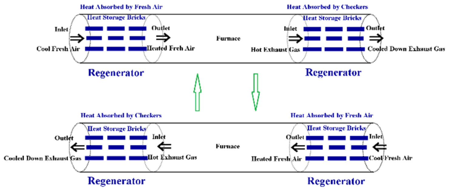
Figure 6.
Phases of our tree search.
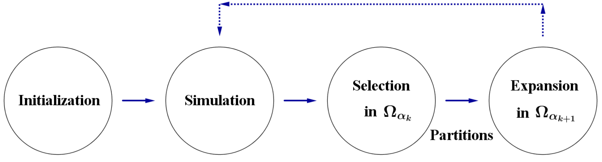
Figure 7.
Two-phase cycle of a fixed-bed heat regenerator.
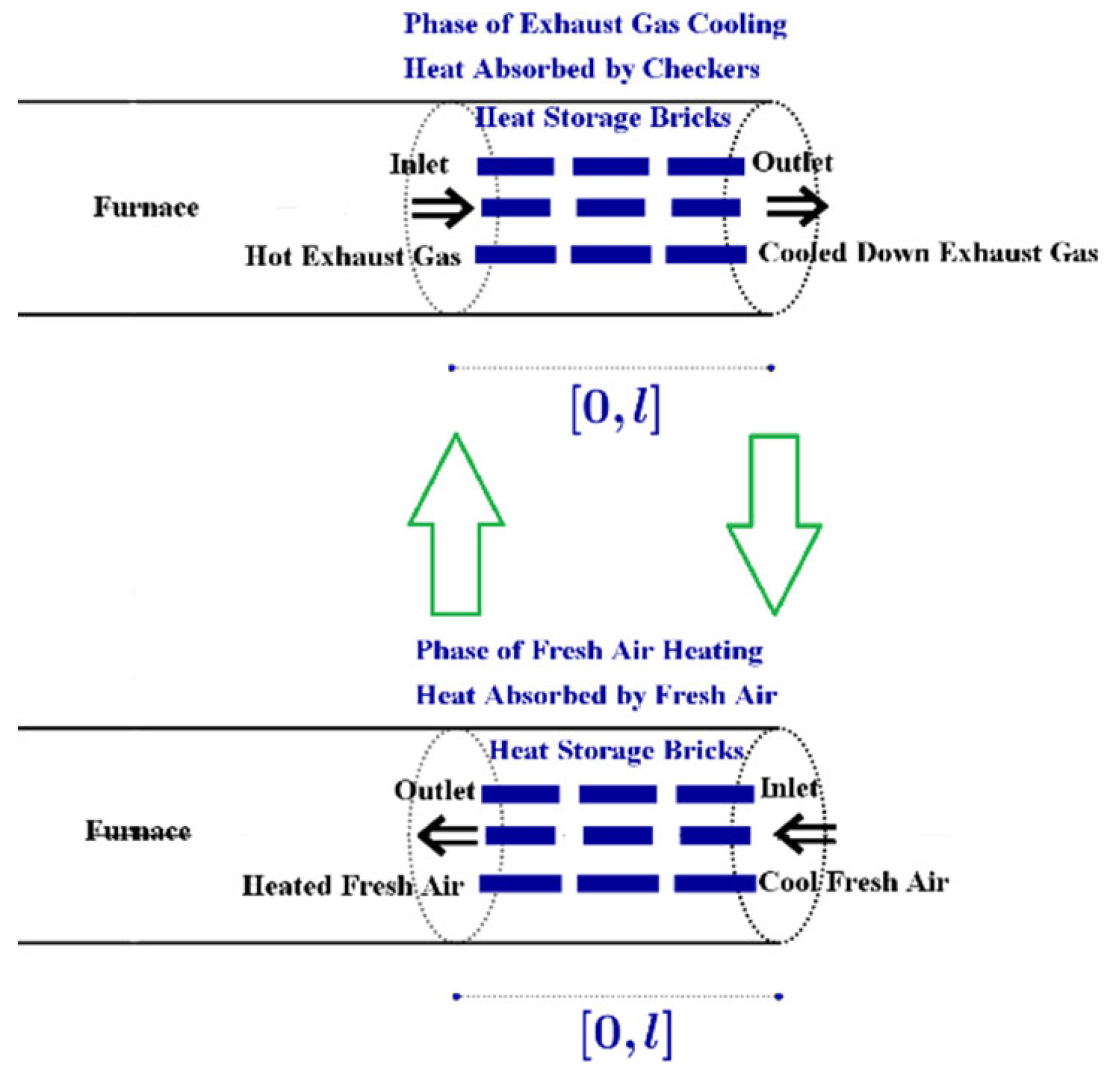
Figure 8.
Comparison of 1-D simulations with 3-D CFD simulations on Ansys Fluent.
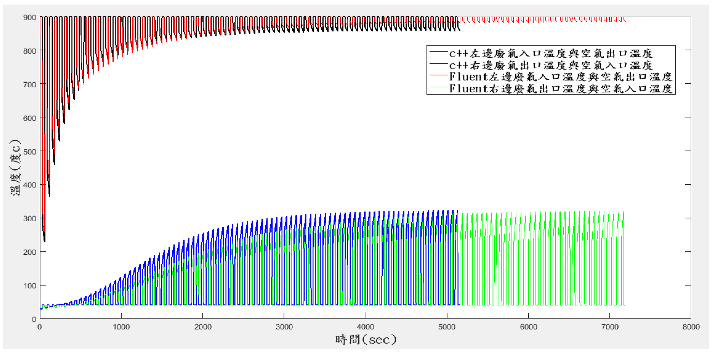
Figure 9.
Algorithm based on our simple tree search with the Mutation Expansion operator.
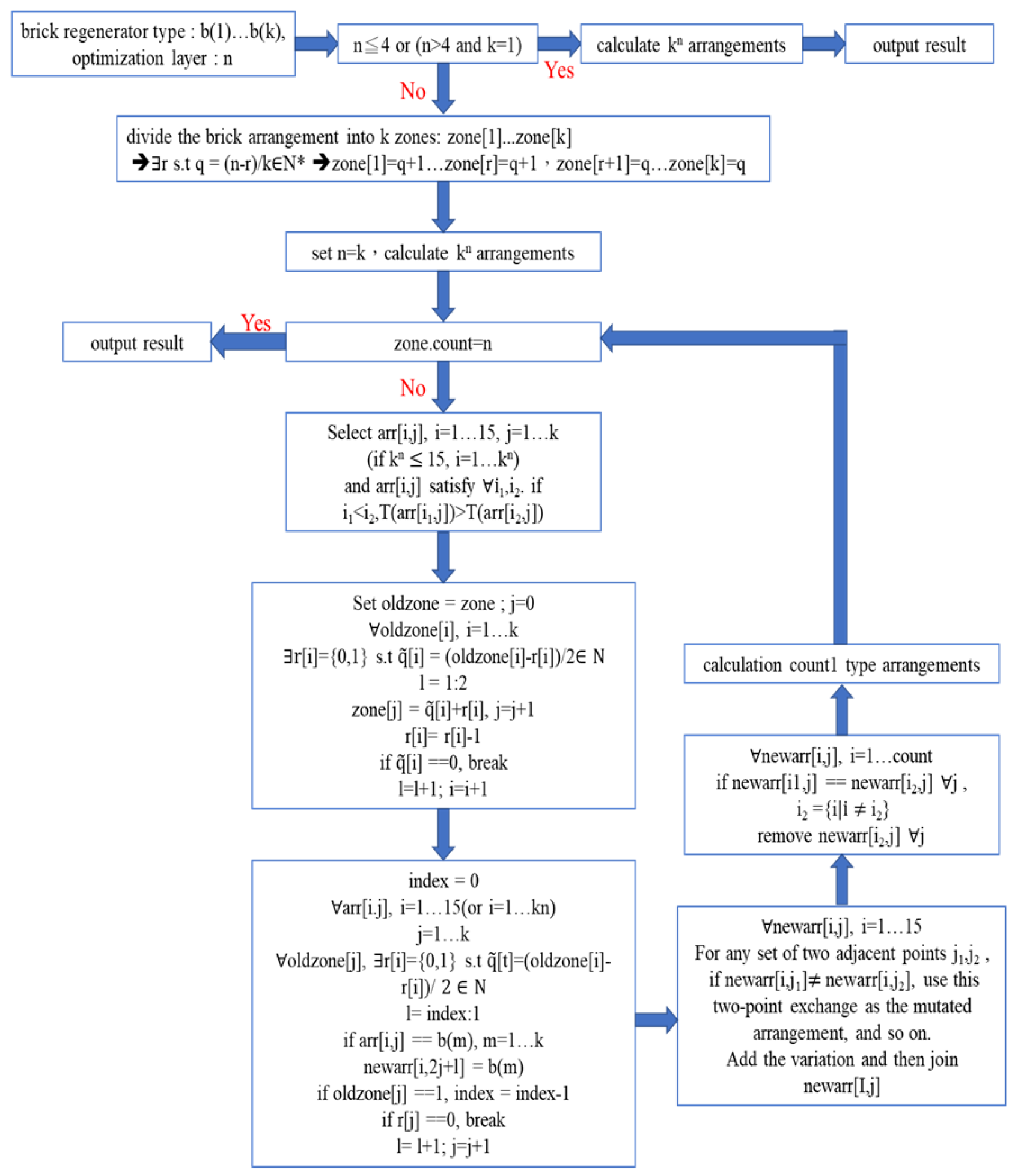

Table 1.
Material parameters of checkers.
| Cordierite | Mullite | |
| size | 150×150×100 | 150×150×100 |
| pore size | 4.9 | 3.0 |
| wall thickness | 1.04 | 0.70 |
| porosity | 0.62 | 0.64 |
| specific surface area | 501 | 853 |
| density | 2200 | 2500 |
| specific heat capacity | 1000 | 1200 |
| thermal conductivity | 2 | 2 |
Table 2.
Material parameters of checkers.
| Mullite A | Mullite B | Mullite C | |
| size | 100×100×100 | 150×150×100 | 150×150×100 |
| pore size | 17 | 4 | 6 |
| wall thickness | 0.8 | 1.5 | 2 |
| porosity | 0.182 | 0.524 | 0.524 |
| specific surface area | 42.7 | 523.8 | 349.2 |
| density | 2200 | 2200 | 2200 |
| specific heat capacity | 836 | 836 | 836 |
| thermal conductivity | 1.8 | 1.8 | 1.8 |
Table 3.
Operating parameters for Experiments 1 and 2.
| Total horizontal length of stacking | 200 |
| Total vertical length of stacking | 300 |
| Natural gas flow | 17.65 |
| Air-fuel ratio | 15.9 |
| Inlet temperature of exhaust gas | 1050 (Experiment 1) 1150 (Experiment 2) |
| Inlet temperature of fresh air | 313 |
| Time of Phase Switch | 30 |
Table 4.
Optimization by the usual complete search method.
| Rank | Arrangements of checkers | Inlet temperature of exhaust gas (℃) | Outlet temperature of exhaust gas (℃) | Waste Heat Recovery Ratio (%) |
| 1 | 886.82 | 264.67 | 67.88 | |
| 2 | 886.28 | 286.82 | 65.82 | |
| 3 | 885.82 | 259.48 | 63.77 |
Table 5.
Optimization by our simple tree search method.
| Rank | Arrangements of checkers | Inlet temperature of exhaust gas (℃) | Outlet temperature of exhaust gas (℃) | Waste Heat Recovery Ratio (%) |
| 1 | 886.82 | 264.67 | 67.88 | |
| 9 | 885.14 | 284.35 | 61.72 | |
| 11 | 885.08 | 286.08 | 60.70 |
Disclaimer/Publisher’s Note: The statements, opinions and data contained in all publications are solely those of the individual author(s) and contributor(s) and not of MDPI and/or the editor(s). MDPI and/or the editor(s) disclaim responsibility for any injury to people or property resulting from any ideas, methods, instructions or products referred to in the content. |
© 2025 by the authors. Licensee MDPI, Basel, Switzerland. This article is an open access article distributed under the terms and conditions of the Creative Commons Attribution (CC BY) license (http://creativecommons.org/licenses/by/4.0/).
Copyright: This open access article is published under a Creative Commons CC BY 4.0 license, which permit the free download, distribution, and reuse, provided that the author and preprint are cited in any reuse.


