Submitted:
15 January 2025
Posted:
16 January 2025
You are already at the latest version
Abstract
Thermodynamic equipment efficiency continues to be a topical area of research, especially at the advent of 3D printing of compact heat exchangers (HX). The innovative equipment should address wholistic efficiency concerns (thermodynamic, sustainable, economic). This study dynamically simulated a CO2 (R744) transcritical vapor compression refrigeration system fitted with novel hy-brid Triply Periodic Minimal Surface heat exchangers and compared with it to a tubular HX system on energy, exergy, exergoeconomic, economic and environmental performance. The models were run in MATLAB, which called their Simulink dynamic simulations. Key findings were; improved heat transfer effectiveness due to the material’s intricate shape, exergy efficiency is 5.79% better, initial investment savings is 16.49%, CO2 penalty cost rate reduction of 15.04%, and overall exergy cost rate reduction of 40.83%. The implications of these findings are that the proposed HX achieves more surface area and less material volume for heat transfer equivalent to a bigger pipe HX, hence more economic at less environmental impact and reduced irreversibilities.
Keywords:
hybrid Triply Periodic Minimal Surface heat exchangers
; transcritical CO2 R744
; exergoeconomic
; vapor compression refrigeration
; exergy
; hybridization
1. Introduction
Carbon dioxide CO2 refrigeration continues to gain popular research and experimental relevance. Dilshad et al. [1] reported that between the years of 2013 and 2018, there has been an overwhelming increase (north of 550%) in transcritical CO2 refrigeration systems globally. The authors estimate that the total number of these systems in operation are approximately 20,000, and that they are mostly in Europe (more than 16,000) and Japan (more than 3,500). Research on these systems centers around their energy and exergy efficacy, compactness, economy and environmental sustainability.
One index of efficiency is the improvement of cooling capacity and efficiency, in which cycle modifications have been focused on the internal heat exchanger (IHX). Prominent studies on the IHX configuration have been carried out by among others Boewe et al. [2], Wang et al. [3], Nilesh et al. [4]. Of particular interest is the experimental study that showed that an IHX in a transcritical cycle at a room temperature of 318.15K (45OC) and an evaporation temperature of 278.15K (5OC), can increase the Coefficient of performance (COP) by 5.71% and exergy efficiency by 5.05%. A IHX cycle has yielded low compressor power at conditions: 100 bar (high pressure side) and less than 273.15K evaporation temperature. Among some of their other findings, there has been a 25% cycle efficiency improvement due to fitting an IHX to the cycle. Over and above energy and exergy assessment, some studies have incorporated exergoeconomic, economic and environmental analysis. This wholistic approach enables a more realistic diagnosis, performance monitoring, and optimization of the design and operation of an energy system[5,6].
Printed circuit heat exchangers (PCHEs) have dominated the research space for decades, but recently, the debut of Triply periodic minimal surface heat exchangers (TPMS HXs) has significantly changed the ball game of numerical and experimental thermal modeling. The technology of TPMS HXs is actively being numerically and experimentally modelled across a wide range of applications. TPMS HXs have high surface area-to-volume ratio [7,8,9], which results in compactness and better space economy, rendering them applicable across multiple technologies, among them; desalination viz. membrane distillation [10,11,12,13,14,15], thermal energy storage in phase change materials [16,17,18,19], thermal management (battery cooling), hydrogen storage technology [20].
The performance evaluation coefficient (PEC), which is the ratio between Nu (Nu/Nu0) and friction factor (f/f0)1/3, proved to be over 90 % better on the Diamond, Gyroid and IWP (I-graph and Wrapped Package-graph) HXs than on the PCHE HX [21]. A 29 % improved thermal effectiveness on a Brayton sCO2 cooler was recorded by Liang et al. [22], better than on the PCHE. Iyer et al. [23] and Yan et al. [21]’s comparative study on pressure drop and heat transfer of TPMS HXs against a pipe HX showed that TPMS HXs performed 13 times better than a pipe HX. Conclusively, the authors found that the Schwarz-D based HX was 3 – 10 more compact than a tubular HX in terms of heat transfer effectiveness.
There is a more advanced study of TPMS HXs in the area of hybridizing two or three TPMSs into one by Yan et al. [24]. Their findings showed that hybridizing primitive, gyroid and diamond TPMS improved both heat transfer and pressure drop. There is still a need to investigate hybridized TPMS HXs and their potential performance in thermal and power systems.
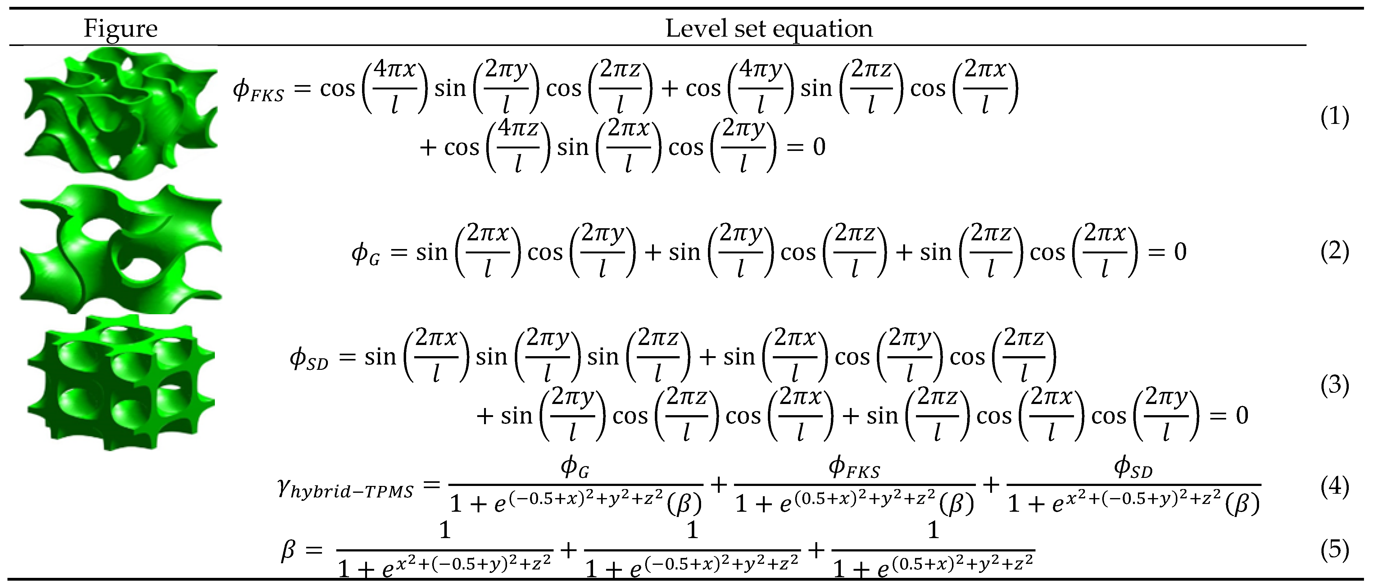
On the basis of the above, and following our latest hypothesis that hybridized TPMS HXs may hold the answer to highly efficient HXs [25], this paper seeks to advance the same narrative by way of numerical models. In this article, an energy, exergy, exergoeconomic, economic and environmental (5Es) study of two transcritical CO2 Refrigeration cycle configurations is presented. One configuration/system has tubular HXs on all its HXs, while the other configuration/system has a hybridized TPMS HXs (Figure 1) in all its HXs. The hybrid TPMS HX was made by combining Gyroid (Equation 1 by von Schenering and Nesper [26]), Schwarz-Diamond (Equation 2 by Michielsen and Kole [27]) and Fischer Koch S (Equation 3, [26]), resulting in Equation 4 of Letlhare-Wastikc and Yang [28] as rendered in Figure 1. A good example of how the hybrid HX can look like after 3D printing is in Figure 2. A more detailed general methodology for TPMS topology hybridization is in Yang et al. [29] and Al Ketan and Abu Al Rub [30]. In this study, the refrigeration system that has been fitted with the Equation 4 hybrid TPMS is abbreviated as TPMS HX and the baseline as pipe HX or tubular HX. The analysis was performed by varying the hydraulic diameters to answer the objective question of how it affects the cooling rate (), exergy efficiency (), overall exergy cost rate (), Pay back period (PBP) and the CO2 penalty cost rate (). Our discussions of the results build to a scientifically justified conclusion.
The sections of this study are presented in the order: Materials and Methods (system description, parameters, operating and initial conditions, control strategy, models), Results and discussions and finally the conclusion and recommendations for future work.
2. Materials and Methods
2.1. System Description
In terms of cycle configuration, the two CO2- (R744) based transcritical refrigeration configurations are the same except that one is fitted with TPMS HXs on its gas cooler, evaporator and internal heat exchanger (IHX), the other one is fitted with pipe/tubular HXs on those same system components. The other components in the system are the compressor and the expansion valve. The cycle schematic and the Ph diagram (Figure 3) show states 1 through to 6 in which the CO2 passes through the cycle. The IHX improves both COP of refrigeration and COP of exergy by raising subcooling (at gas cooler exit) on the high pressure side and by increasing superheating (at evaporator exit) on the low pressure side. The HXs are made from the Aluminum-Silicon-Magnesium alloy (AlSi10Mg) whose thermal qualities are in Table 2. Table 3 presents the geometric and thermohydraulic

Table 1.
Equations of the standard TPMS’s and of the hybrid TPMS.
 |
parameters of the HXs. The material AlSi10Mg was chosen for its good strength and hardness, excellent corrosion resistance, good weldability and machinability, widely available, relatively low cost [32], and 3D printability into a compact HX.
The area, volume, density and heat capacity of the compartment contents (food), and the environment temperature are given in Table 4 and are kept constant in both configurations.
2.2. Parameters, Operating and Initial Conditions
A dynamic model was setup in Simulink on MATLAB R2020a. Table 4 presents the operating conditions, parameters and initial conditions on which both systems/configurations are based. For air, specific heat () is 1000 J/kg.K and density is () is 1.2 kg/m3. For the TPMS HX model, the code loops through all the unit cell lengths, while for the tubular HX, it loops through all the hydraulic diameters over 25,000 seconds.
2.3. Control Strategy
The expansion valve opening (in meters) is controlled by a simple proportional integrator (PI) controller between the output saturation upper limit of 0.1 to 0.02 and lower limit of 0.0001 to 0.02, to maintain the difference between the outlet and inlet temperature of the evaporator at 3K for superheating.
The compressor RPM is controlled by a simple PI controller between the output saturation upper limit of 4000 to 2000 and lower limit of 0 to 2000, to maintain the compartment temperature at 278.15K.
The following simplifications were applied to the model;
- The isentropic efficiencies are fixed,
- Flow is laminar,
- Evaporator outlet of CO2 is saturated vapor,
- Expansion process is isenthalpic.
2.4. Mathematical Models
The mathematical models are presented in the order: energy, exergy, exergoeconomic, economic and environmental. Their parameters and corresponding evaluation indexes are as shown in Figure 4 as (), exergy efficiency (), overall exergy cost rate (), Pay back period (PBP) and the CO2 penalty cost rate () respectively. They shall be elaborated upon as and when they are dealt with.
2.4.1. Energy Model
The energy models will be based on the governing equations of conservation of mass and energy. While their mass and energy balances are in Equations 6 and 7, they are comprehensively given per component in Table 5.
2.4.2. Exergy Model
We need to determine the maximum useful work which can be harnessed from our system as it reversibly comes into equilibrium with its environment [34]. The total exergy (availability) of a system has physical, chemical, kinetic, and potential exergy. An expansion of the exergy models is in Table 5. Given that exergy is:
We proceed as below if there are no velocity, level changes and chemical changes in the system:
Therefore, the physical exergy can be calculated with the following equation:
The enthalpy, entropy and temperature with 0 subscript are at dead state conditions (at 289.15K and 1.01 MPa). Below is the exergy balance of the system, where there is fuel exergy (F,tot), product exergy (P,tot), destruction exergy (D,k), and exergy loss (L,tot):
Neglecting the exergy loss term, the exergy balance equation for each system component is given by:
The exergy efficiency is given by:
2.4.3. Exergoeconomic Model
The fundamental principles of thermoeconomics states that all exergetic costs are associated with their corresponding exergy streams [35]. The exergertic cost balance equation for all or any component is thus:
The indices of the exergoeconomic model as per specific exergy cost method (SPECO), are the exergoeconomic factor (f) and overall exergy cost rate (Ctotal) as follows:
The expansion of the exergy balance equation is given for each equipment in Table 6. The exergy destruction related costs (), exergy loss related costs (), and capital costs (), (all per equipment k) are given below. However, exergy loss related costs are negligible and zero in this system.
The capital recovery factor (CRF) is given by:
Where PECk is the purchase equipment cost as given in Table 6, ϕ is the maintenance factor at 1.06, i is the interest rate at 2.73% [36], n is the service life at 15 years and N is the annual operation hours at 7500.
The PECref is accordingly adjusted from the reference year (2001) to the current year (2024) based on the 2024 Chemical Plant Cost Index (CEPCI) as in Table 6 given by:
2.4.4. Economic Model
Having dealt with the equipment cost and the systems’ energetic efficiency, it is also important to determine the economic viability of the system. The economic analysis includes the calculation of the total setup cost and annual operation cost of the system [39]. The economic index for this study is Pay Back Period (PBP), which is the ratio of the investment difference to the annual savings in operation. Other costs due to labour and piping are assumed to be 15% of PEC and are added to the PECtotal. The annual maintenance cost (MC) is assumed at 1% of 1.15PECtotal.
The Annual Operational Cost (AOC) is calculated by multiplying the PECfinal by the weighting factor of operational cost (bw) of 0.05 and by the commercial electricity price at 0.1$ per kWh.
2.4.5. Environmental Model
In sustainable modeling, it is important to consider the carbon footprint of engineering solutions on the environment. To this extent, we are including an environmental analysis to reckon the CO2 penalty cost rate related to the electricity consumption of the compressor [33]. The related equation is:
3. Results and Discussion
In this section, the impact of varying hydraulic diameters of the TPMS system on the energy, exergy, exergoeconomic, economic, and environmental performance indexes (in that order) of the Transcritical CO2 (R744) vapor-compression refrigeration system is presented. To accentuate the superior performance of the indexes of this system, it is compared to a pipe based HX baseline system.
Table 7 presents the general overview of the 5Es at the last simulated hydraulic diameter of 0.01078m.
3.1. Energy Analysis as Hydraulic Diameter Increases
In both systems (TPMS and tubular/pipe), the 3D surface plot (Figure 5) shows a significant relationship of the dependency of the evaporator’s cooling capacity on geometric parameters of the heat exchangers, viz. surface area, and hydraulic diameter. In both systems, the evaporator’s cooling capacity increases with the increasing geometric parameters, but the TPMS system being steeper. Besides the geometric intricacies of the TPMS which promotes turbulence and improves heat transfer rate, the TPMS’s superior surface area to volume ratio and the Nu. (27.64 in this case), are other aspects that contribute to better heat transfer rate.
3.2. Effect of Hydraulic Diameter Increase on Exergy Efficiency and PBP
As seen in Figure 6, between the first 2 diameters (0.00154 and 0.002567), there is a sharp rise from 67% to 77% in exergy efficiency. While this rise may be exciting at first, it needs to be interpreted with other indices (economic, exergoeconomic and environmental) to give a perspective sense, as shall be done in the subsequent sections.
After the sharp rise, the TPMS system goes upwards in smooth concave until maximum 83.62%, while the tubular system goes slightly down and lazily rises again to a maximum of 77.83%. This is due to reduced irreversibilities in the heat transfer process, caused by the TPMS system’s enhanced surface area-to-volume ratio and turbulence-promoting geometry.
The PBP is a ratio of the investment cost and the annual net income. It is of interest to thermal and refrigeration systems because engineering solutions are only sustainable to societies if thermal efficiencies are economic in investment and operation. Figure 6 shows that for both systems, the first 2 diameters (0.00154 and 0.002567), the PBP is zero, but after that there’s a downward concave growth with increasing hydraulic diameter. However, the TPMS system, at the last hydraulic diameter (0.01078m) is slightly more (1.397 years) than the pipe system (1.268 years), indicating that the investment cost of the TPMS system takes a little over 1.5 months more to be recovered than in a tubular system.
3.3. Effect of Hydraulic Diameter Increase on Capital Investment Cost
In the pursuit of thermally efficient equipment, it is important to consider plant investment cost because it continues to rise year on year due to inflation. For compact heat exchangers like the one proposed in this study, depending on the 3D method used, typically ranges from USD100 to USD150 per kg powder of AlSi10Mg [32].
Figure 7 shows that among all the components, the compressor exhibits the highest capital investment cost for both the tubular and the TPMS systems. While the PEC of the compressor in and of itself is not determined by hydraulic diameter and surface area, they systematically have a bearing on its operation and power rating. For the most part, in both systems, the compressor’s capital cost deeps with a very small and identical gradient as and when the hydraulic diameter increases. However, after hydraulic diameter of 0.006m, the TPMS compressor dips sharper than the tubular compressor, indicating markedly that at this point and beyond, the system’s work input demand reduces due to heat transfer enhancements brought by the increased surface area of the upstream equipment.
The evaporator is the second most expensive component in both systems, followed by the gas cooler. Unlike the compressor, their cost grows as hydraulic diameter increases. This is due to the price per unit material volume, which is a direct function of the hydraulic diameter. The investment cost of the gas cooler and the evaporator is higher and more rapid in the tubular than in the TPMS system, because it follows the trend of their respective surface area increases as hydraulic diameter increases. This is attributable to the pipe heat exchanger’s surface area-to-volume ratio, which needs more surface area (consequently more material volume) to match the growing heat transfer demands brought by the increasing diameter. It must be emphasized that of all the components, the cost of the evaporator is the most responsive (upward) to hydraulic diameter, indicating that the evaporator’s hydraulic diameter has more bearing on its cost than the other equipment.
The rest of the equipment show negligible upward gradients, and the cost of the pipe system is still marginally higher than the TPMS system. This is because hydraulic diameter doesn’t cause a significant change in the surface area, which is a direct function of the material cost per material volume.
3.4. Effect of Hydraulic Diameter Increase on Exergy Cost Rate
Exergy cost rate (in USD/hr) quantifies/evaluates the economic costs of the system’s irreversibilities (energy losses and inefficiencies), or the cost associated with the destruction of exergy over time.t of as the rate at which exergy is irreversibly lost from a system due to inefficiencies. Due to their nature of operation, the expansion valve and the compressor are always the largest contributors of irreversibilities, hence of exergy destruction.
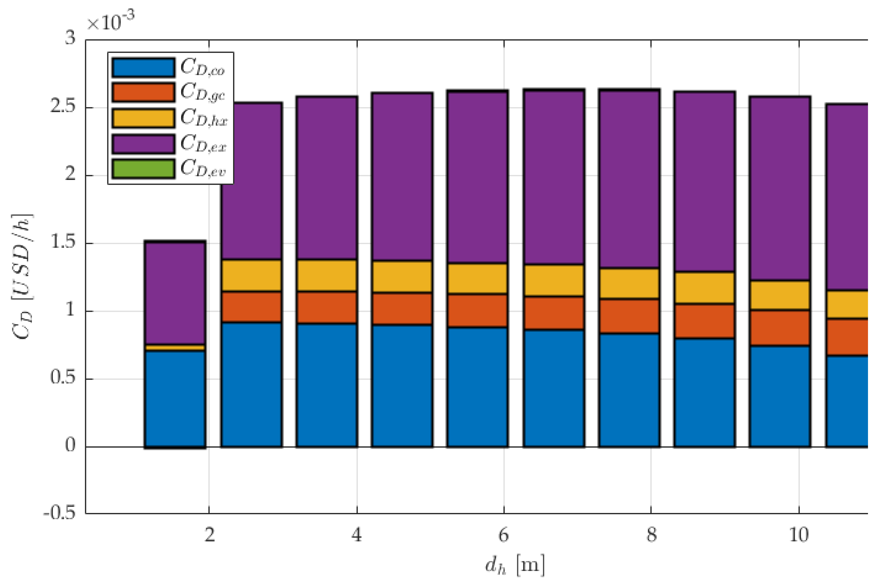
In Figure 8, it is clear that for both systems, the expansion valve is the highest, followed by the compressor. For all equipment, the TPMS system recorded lower values of exergy cost rate than the tube HX, proving to be have less losses, hence more efficient overall. While the losses in the IHX and the gas cooler remain almost constant as hydraulic diameter increases, they are also almost identical between the two systems, indicating that the TPMS has contributed insignificant exergy cost rate efficiency to these two pieces of equipment. However, in the compressor and the expansion valve, we are witnessing impressive reduction of exergy cost rate in the TPMS system, indicating that irreversibilities lessen as hydraulic diameter increases. At the final hydraulic diameter, the percentage improvement done by the TPMS HX in the expansion valve is 21.77% and in the compressor is 99%. For an alternative view, a stacked bar chart is provided in Appendix Figure A2 and Figure A3.
3.5. Effect of Hydraulic Diameter Increase on Environmental and Overall Exergy Cost
As the compressor runs, it requires some electrical energy, and a sustainable analysis is not complete without considering the amount of CO2 released into the environment due to this operation. In our case it is presented in Figure 9 in terms of USD per hour of operation, and is termed CO2 penalty cost rate. In both systems, we notice an initial sharp increase from the first to the second hydraulic diameter, from 36.3 to 46.58 and from 35.96 to 46.4 for the TPMS and the tube HX respectively. This is due to the high energy demands at smaller hydraulic diameter, which intensifies exergy destruction and cost per unit efficiency – these in turn have a direct bearing on the compressor energy demand, manifesting in high CO2 penalty cost rate. We however see a good downward trend developing beyond the second on both systems. The TPMS model demonstrates a more rapid decline, concluding at 36.38 while the tube HX concludes higher at 42.82. The faster decline for the TPMS is due to its superior thermohydraulic performance, which enhances system efficiency and reduces irreversibilities, thereby minimizing cumulative environmental and operational costs at larger .
Overall exergy cost rate (USD/hr) is the sum of the investment cost and all the exergy cost rate of all the equipment of the system. By extension, this is the overall cost of running the refrigeration system, being a combination of both initial capital costs and the ongoing operational costs due to inefficiencies. Figure 9 shows an initial rise in both systems, indicating a high material demand at smaller , but less material demand and less operational costs as increases. The final figures of for TPMS HX and tubular HX systems are 0.001507 and 0.002547, respectively. This 40.83% reduction in is indicative of the TPMS HX system’s superior thermohydraulic performance, which enhances system efficiency and reduces irreversibilities, thereby minimizing cumulative operational costs at larger .
4. Conclusion
Our conclusions align with each of our earlier stated objectives; to conduct an energy, exergy, exergoeconomic, economic and environmental (5Es) study with the respective indices of cooling rate (), exergy efficiency (), overall exergy cost rate (), Pay back period (PBP) and the CO2 penalty cost rate (). While we have discussed the causal trends f increasing on all the indices under study, the percentage effect in this section is discussed at the terminal of 0.01181m. Following the discussion in the results section, we aver that;
- Compared to the TPMS, the tubular heat exchanger has a comparatively limited surface area and surface area to volume ratio for the same hydraulic diameter, resulting in a lower rate of increase in cooling capacity.
- The novel TPMS design provides greater surface area for heat transfer without proportionally increasing the overall material volume, thereby reducing the capital cost of 3D printing/manufacturing of AlSi10Mg for the HXs.
- The novel TPMS design has a better and positive exergy efficiency response rate to hydraulic diameter, and is 5.79% better than the pipe system.
- The compressor is the most expensive component. The evaporator is the most responsive to hydraulic diameter variations, indicating that a designer needs to be careful about its tradeoff balances between its cooling capacity and its effect on the system’s economics. The overall initial investment savings that come with using the TPMS HXs is 16.49%, which is a true testament the compactness and space economy of the TPMS against the pipe HX.
- The PBP analysis shows that the capital investment cost of both systems take longer to be recovered as hydraulic diameter grows and that at the final hydraulic diameter, the TPMS system’s capital investment cost takes a little over 1.5 months more to be recovered than in a tubular system.
- For all equipment, the TPMS system recorded lower values of exergy cost rate than the tube HX, proving to have less losses, hence more efficient in overall operation.
- The TPMS HXs reduces the CO2 penalty cost rate by 15.04%.
- The 40.83% reduction of in using TPMS HX systems points to the adverse material volume reduction and operational irreversibilities reduction savings over counterpart system.
The novel TPMS heat exchanger has impressive results, but for future work, optimization studies can be performed to reduce investment cost and irreversibilities while maximize cooling capacity.
Author Contributions
Conceptualization, K.L.W.; methodology, K.L.W.; software, X.Y.; validation, K.L.W.; formal analysis, X.Y. and K.L.W.; investigation, K.L.W.; resources, X.Y.; data curation, K.L.W.; writing—original draft preparation, K.L.W.; writing—review and editing, X.Y. and K.L.W.; visualization, K.L.W.; supervision, X.Y.; project administration, X.Y. All authors have read and agreed to the published version of the manuscript.
Funding
This research received no external funding.
Data Availability Statement
Data will be made available on request by emailing the corresponding author.
Conflicts of Interest
The authors declare no conflicts of interest.
Appendix A
Table A1.
Darcy friction factor and Nusselt number at Prandtl number of 6.97 [23].
Table A1.
Darcy friction factor and Nusselt number at Prandtl number of 6.97 [23].
| Parameter | TPMS | Range of Re |
|---|---|---|
| Nusselt number | 10 < Re < 140 | |
| 25 < Re < 250 | ||
| 15 < Re < 300 | ||
| Darcy friction factor* | 10 < Re < 140 | |
| 10 < Re < 140 | ||
| ) | 10 < Re < 140 |
*Fanning friction factor is
Figure A2.
Exergy destruction cost rate of the TPMS system.
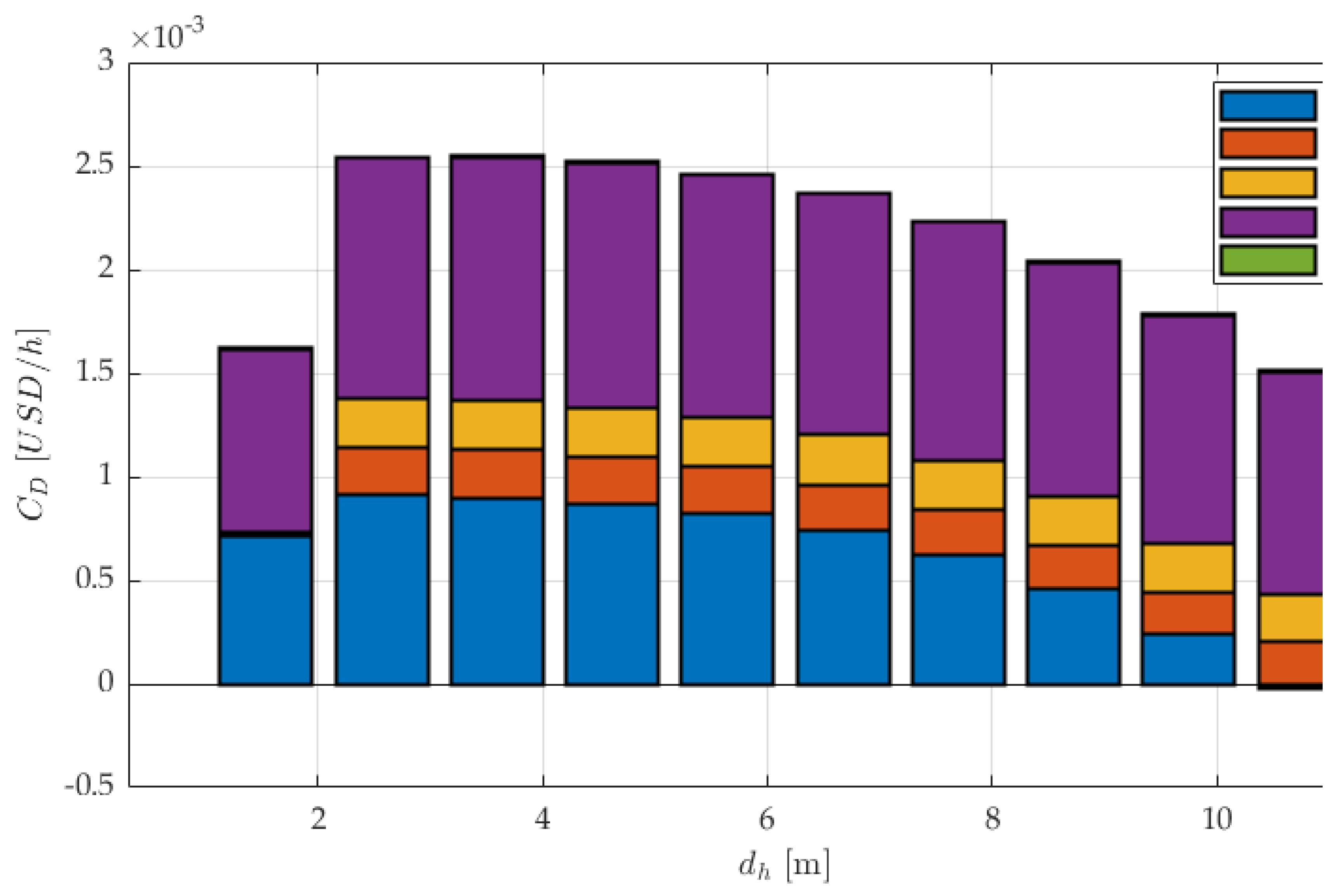
Figure A3.
Exergy destruction cost rate of the Tubular system.
References
- Dilshad, S.; Kalair, A.R.; Khan, N. Review of Carbon Dioxide (CO2) Based Heating and Cooling Technologies: Past, Present, and Future Outlook. Int. J. Energy Res. 2020, 44, 1408–1463. [Google Scholar] [CrossRef]
- Boewe, D.E.; Bullard, C.W.; Yin, J.M.; Hrnjak, P.S. Contribution of Internal Heat Exchanger to Transcritical R-744 Cycle Performance. HVAC R Res. 2001, 7, 155–168. [Google Scholar] [CrossRef]
- Wang, Z.; Gong, Y.; Wu, X.H.; Zhang, W.H.; Lu, Y.L. THERMODYNAMIC ANALYSIS AND EXPERIMENTAL RESEARCH OF TRANSCRITICAL CO2 CYCLE WITH INTERNAL HEAT EXCHANGER AND DUAL EXPANSION. Int. J. Air-Cond. Refrig. 2013, 21, 1350005. [Google Scholar] [CrossRef]
- Purohit, N.; Gupta, D.K.; Dasgupta, M.S. Experimental Investigation of a CO2 Trans-Critical Cycle with IHX for Chiller Application and Its Energetic and Exergetic Evaluation in Warm Climate. Appl. Therm. Eng. 2018, 136, 617–632. [Google Scholar] [CrossRef]
- Mehrdad, S.; Dadsetani, R.; Amiriyoon, A.; Leon, A.S.; Reza Safaei, M.; Goodarzi, M. Exergo-Economic Optimization of Organic Rankine Cycle for Saving of Thermal Energy in a Sample Power Plant by Using of Strength Pareto Evolutionary Algorithm II. Processes 2020, 8, 264. [Google Scholar] [CrossRef]
- Dadsetani, R.; Sheikhzadeh, GH.A.; Safaei, M.R.; Alnaqi, A.A.; Amiriyoon, A. Exergoeconomic Optimization of Liquefying Cycle for Noble Gas Argon. Heat Mass Transf. 2019, 55, 1995–2007. [Google Scholar] [CrossRef]
- Al-Ketan, O.; Abu Al-Rub, R.K. Multifunctional Mechanical Metamaterials Based on Triply Periodic Minimal Surface Lattices. Adv. Eng. Mater. 2019, 21, 1900524. [Google Scholar] [CrossRef]
- Li, W.; Yu, G.; Yu, Z. Bioinspired Heat Exchangers Based on Triply Periodic Minimal Surfaces for Supercritical CO2 Cycles. Appl. Therm. Eng. 2020, 179, 115686. [Google Scholar] [CrossRef]
- Torquato, S.; Donev, A. Minimal Surfaces and Multifunctionality. Proc. R. Soc. Lond. Ser. Math. Phys. Eng. Sci. 2004, 460, 1849–1856. [Google Scholar] [CrossRef]
- Termpiyakul, P.; Jiraratananon, R.; Srisurichan, S. Heat and Mass Transfer Characteristics of a Direct Contact Membrane Distillation Process for Desalination. Desalination 2005, 177, 133–141. [Google Scholar] [CrossRef]
- Chordia, L.; Portnoff, M.A.; Green, E.; Southwest Research Institute; Knolls Atomic Power Laboratory High Temperature Heat Exchanger Design and Fabrication for Systems with Large Pressure Differentials; 2017; p. DE-FE0024012, 1349235.
- Yun, Y.; Ma, R.; Zhang, W.; Fane, A.G.; Li, J. Direct Contact Membrane Distillation Mechanism for High Concentration NaCl Solutions. Desalination 2006, 188, 251–262. [Google Scholar] [CrossRef]
- Lawson, K.W.; Lloyd, D.R. Membrane Distillation. J. Membr. Sci. 1997, 124, 1–25. [Google Scholar] [CrossRef]
- Alkhudhiri, A.; Darwish, N.; Hilal, N. Membrane Distillation: A Comprehensive Review. Desalination 2012, 287, 2–18. [Google Scholar] [CrossRef]
- Thomas, N.; Mavukkandy, M.O.; Loutatidou, S.; Arafat, H.A. Membrane Distillation Research & Implementation: Lessons from the Past Five Decades. Sep. Purif. Technol. 2017, 189, 108–127. [Google Scholar] [CrossRef]
- Qureshi, Z.A.; Addin Burhan Al-Omari, S.; Elnajjar, E.; Al-Ketan, O.; Al-Rub, R.A. On the Effect of Porosity and Functional Grading of 3D Printable Triply Periodic Minimal Surface (TPMS) Based Architected Lattices Embedded with a Phase Change Material. Int. J. Heat Mass Transf. 2022, 183, 122111. [Google Scholar] [CrossRef]
- Kumaresan, V.; Chandrasekaran, P.; Nanda, M.; Maini, A.K.; Velraj, R. Role of PCM Based Nanofluids for Energy Efficient Cool Thermal Storage System. Int. J. Refrig. 2013, 36, 1641–1647. [Google Scholar] [CrossRef]
- Gado, M.G.; Ookawara, S.; Nada, S.; Hassan, H. Performance Investigation of Hybrid Adsorption-Compression Refrigeration System Accompanied with Phase Change Materials − Intermittent Characteristics. Int. J. Refrig. 2022, 142, 66–81. [Google Scholar] [CrossRef]
- Gado, M.G.; Hassan, H. Energy-Saving Potential of Compression Heat Pump Using Thermal Energy Storage of Phase Change Materials for Cooling and Heating Applications. Energy 2023, 263, 126046. [Google Scholar] [CrossRef]
- Zhao, C.; Liu, J.; Li, B.; Ren, D.; Chen, X.; Yu, J.; Zhang, Q. Multiscale Construction of Bifunctional Electrocatalysts for Long-Lifespan Rechargeable Zinc–Air Batteries. Adv. Funct. Mater. 2020, 30, 2003619. [Google Scholar] [CrossRef]
- Yan, K.; Wang, J.; Li, L.; Deng, H. Numerical Investigation into Thermo-Hydraulic Characteristics and Mixing Performance of Triply Periodic Minimal Surface-Structured Heat Exchangers. Appl. Therm. Eng. 2023, 230, 120748. [Google Scholar] [CrossRef]
- Liang, D.; Yang, K.; Gu, H.; Chen, W.; Chyu, M.K. The Effect of Unit Size on the Flow and Heat Transfer Performance of the “Schwartz-D” Heat Exchanger. Int. J. Heat Mass Transf. 2023, 214, 124367. [Google Scholar] [CrossRef]
- Iyer, J.; Moore, T.; Nguyen, D.; Roy, P.; Stolaroff, J. Heat Transfer and Pressure Drop Characteristics of Heat Exchangers Based on Triply Periodic Minimal and Periodic Nodal Surfaces. Appl. Therm. Eng. 2022, 209, 118192. [Google Scholar] [CrossRef]
- Yan, G.; Sun, M.; Zhang, Z.; Liang, Y.; Jiang, N.; Pang, X.; Song, Y.; Liu, Y.; Zhao, J. Experimental Study on Flow and Heat Transfer Performance of Triply Periodic Minimal Surface Structures and Their Hybrid Form as Disturbance Structure. Int. Commun. Heat Mass Transf. 2023, 147, 106942. [Google Scholar] [CrossRef]
- Letlhare-Wastikc, K.; Yang, X. Hybridized Triply Periodic Minimal Surface Recuperators in CSP Super-Critical CO2 Recompressed Brayton Cycles – Review and Avant-Garde Pro-Spects 2024.
- von Schnering, H.G.; Nesper, R. Nodal Surfaces of Fourier Series: Fundamental Invariants of Structured Matter. Z. Für Phys. B Condens. Matter 1991, 83, 407–412. [Google Scholar] [CrossRef]
- Michielsen, K.; Kole, J.S. Photonic Band Gaps in Materials with Triply Periodic Surfaces and Related Tubular Structures. Phys. Rev. B 2003, 68, 115107. [Google Scholar] [CrossRef]
- Letlhare-Wastikc, K.; Yang, X. Triply Periodic Minimal Surface Hybridization and Novel Thin Walled AlSi10Mg Heat Exchanger Modeling for Sustainable Energy Applications 2024.
- Yang, N.; Wang, S.; Gao, L.; Men, Y.; Zhang, C. Building Implicit-Surface-Based Composite Porous Architectures. Compos. Struct. 2017, 173, 35–43. [Google Scholar] [CrossRef]
- Al-Ketan, O.; Abu Al-Rub, R.K. MSLattice: A Free Software for Generating Uniform and Graded Lattices Based on Triply Periodic Minimal Surfaces. Mater. Des. Process. Commun. 2021, 3. [Google Scholar] [CrossRef]
- Kelly, J.P.; Finkenauer, L.R.; Roy, P.; Stolaroff, J.K.; Nguyen, D.T.; Ross, M.S.; Hoff, A.T.; Haslam, J.J. Binder Jet Additive Manufacturing of Ceramic Heat Exchangers for Concentrating Solar Power Applications with Thermal Energy Storage in Molten Chlorides. Addit. Manuf. 2022, 56, 102937. [Google Scholar] [CrossRef]
- MET3DP, D. AlSi10Mg for Metal 3D Printing: A Definitive Guide. Lead. Addit. Manuf. Mater.
- Belman-Flores, J.M.; Rangel-Hernández, V.H.; Pérez-García, V.; Zaleta-Aguilar, A.; Fang, Q.; Méndez-Méndez, D. An Advanced Exergoeconomic Comparison of CO2-Based Transcritical Refrigeration Cycles. Energies 2020, 13, 6454. [Google Scholar] [CrossRef]
- Exergy Economics, E. What Is Exergy?
- Fazelpour, F.; Morosuk, T. Exergoeconomic Analysis of Carbon Dioxide Transcritical Refrigeration Machines. Int. J. Refrig. 2014, 38, 128–139. [Google Scholar] [CrossRef]
- Bu, S.; Yang, X.; Li, W.; Dai, W.; Su, C.; Wang, X.; Liu, X.; Yu, N.; Wang, G. Energy, Exergy, Environmental, and Economic Analyses and Multiobjective Optimization of a DSORC System for Waste Heat Utilization in Low-Concentration Gas Power Generation. Energy 2024, 286, 129647. [Google Scholar] [CrossRef]
- Garousi Farshi, L.; Mahmoudi, S.M.S.; Rosen, M.A. Exergoeconomic Comparison of Double Effect and Combined Ejector-Double Effect Absorption Refrigeration Systems. Appl. Energy 2013, 103, 700–711. [Google Scholar] [CrossRef]
- Maxwell, C. Cost Indices 2020.
- Isik, M.; Bilir Sag, N. Energetic, Economic, and Environmental Analysis of CO2 Booster Refrigeration Systems of Supermarket Application for Türkiye. Sādhanā 2023, 48, 275. [Google Scholar] [CrossRef]
- Mosaffa, A.H.; Farshi, L.G.; Infante Ferreira, C.A.; Rosen, M.A. Exergoeconomic and Environmental Analyses of CO2/NH3 Cascade Refrigeration Systems Equipped with Different Types of Flash Tank Intercoolers. Energy Convers. Manag. 2016, 117, 442–453. [Google Scholar] [CrossRef]
Figure 1.
The hybrid HX in 4 views (a), (b), (c), (d) and the cross sections when diamond, gyroid and FKS are interchanged between the tri-domains [28].
Figure 1.
The hybrid HX in 4 views (a), (b), (c), (d) and the cross sections when diamond, gyroid and FKS are interchanged between the tri-domains [28].
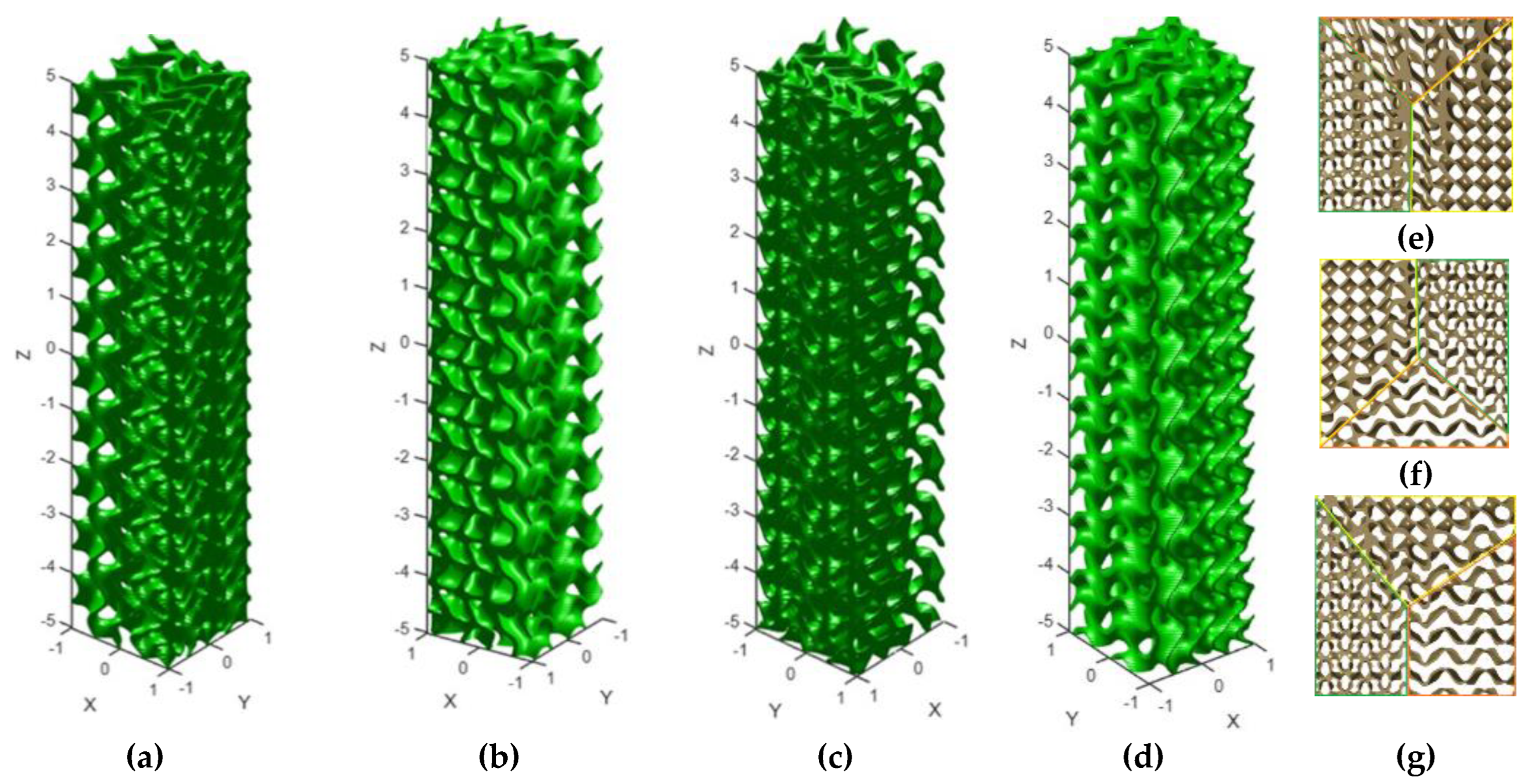
Figure 2.
An example of how the designed TPMS HX can be rendered in 3D print [31].
Figure 2.
An example of how the designed TPMS HX can be rendered in 3D print [31].
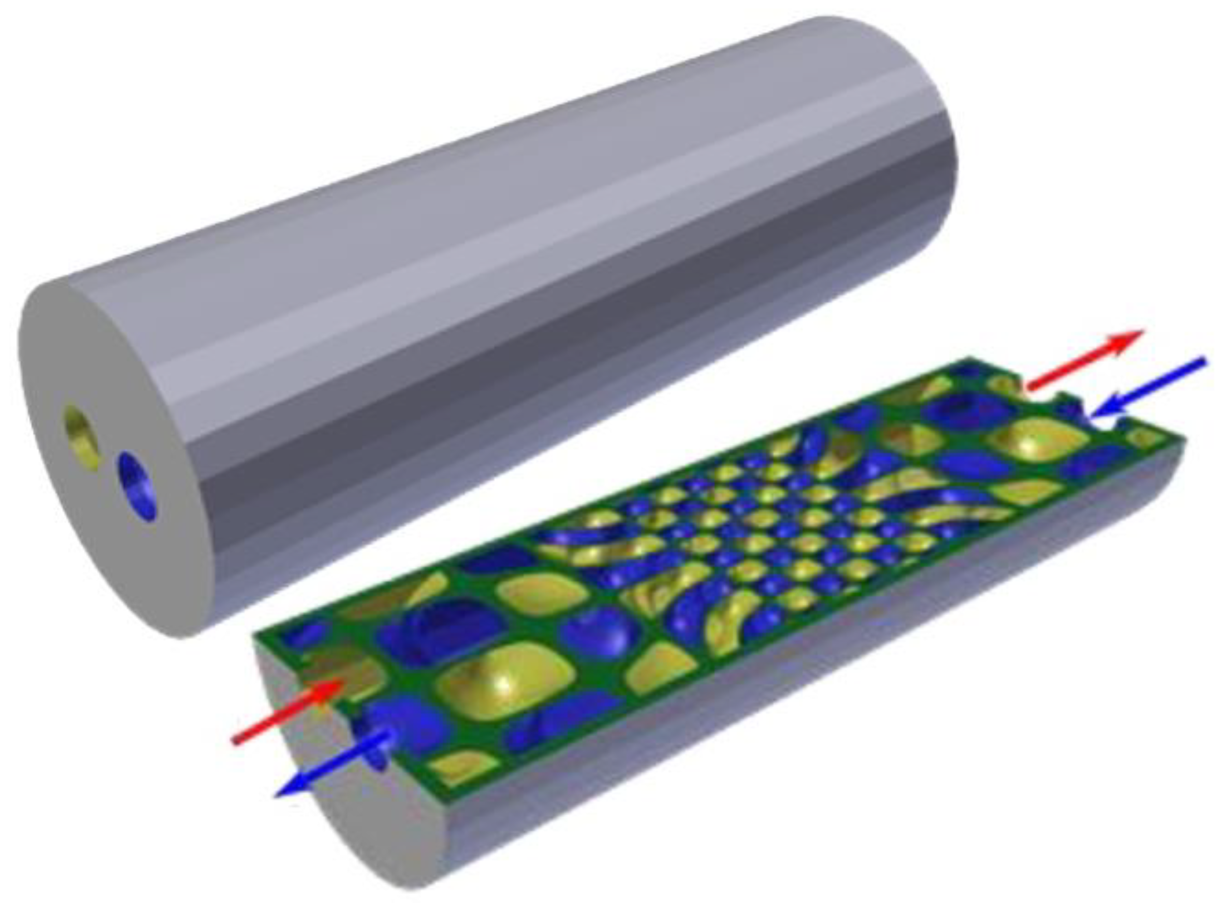
Figure 3.
The cycle schematic and the Ph diagram, edited from [33].
Figure 3.
The cycle schematic and the Ph diagram, edited from [33].
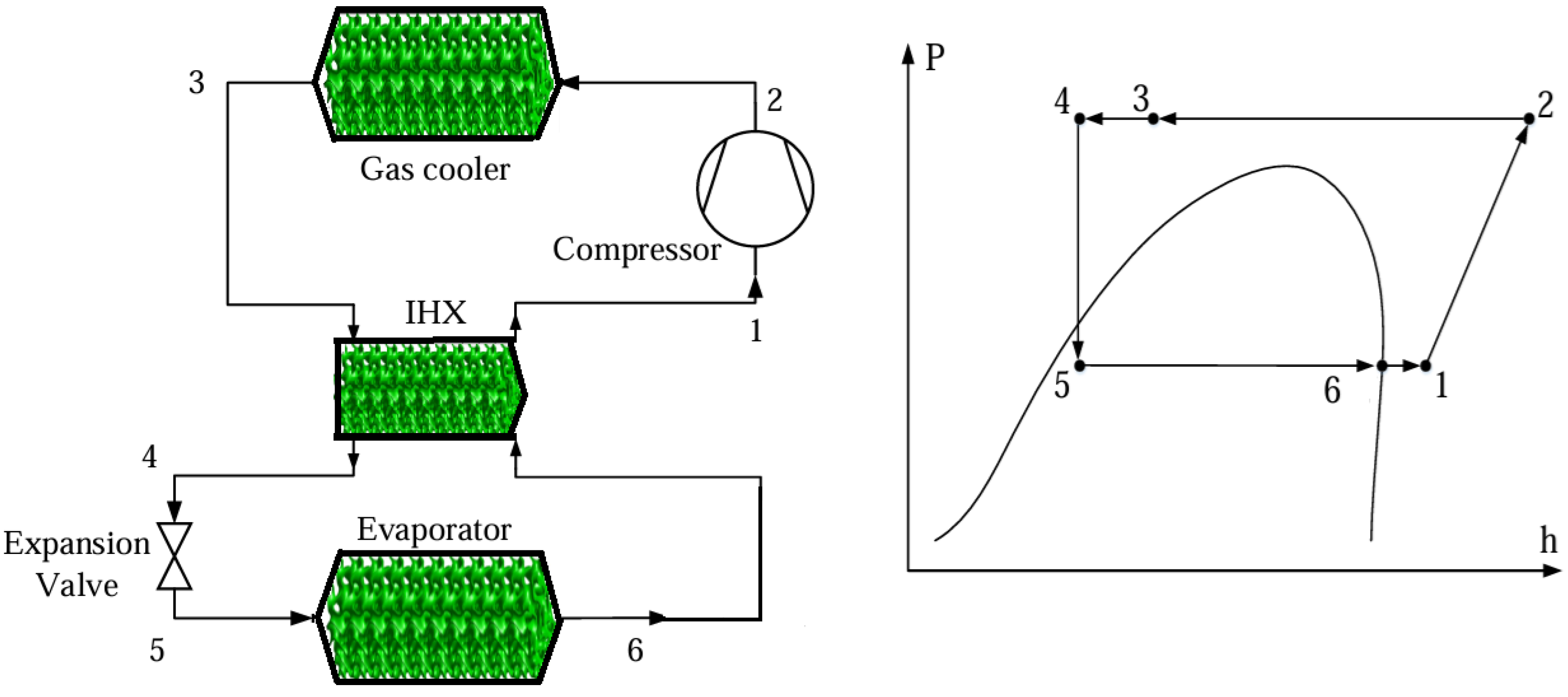
Figure 4.
Modeling flow chart.
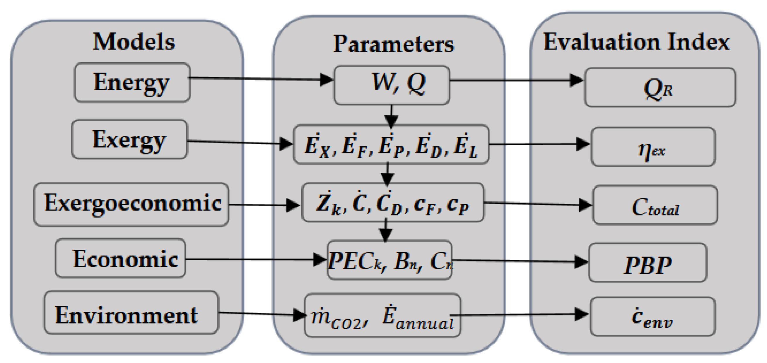
Figure 5.
A 3D plot of the evaporator’s surface area and refrigerating capacity all against hydraulic diameter for the (a) TPMS HX and the (b) tubular HX.
Figure 5.
A 3D plot of the evaporator’s surface area and refrigerating capacity all against hydraulic diameter for the (a) TPMS HX and the (b) tubular HX.
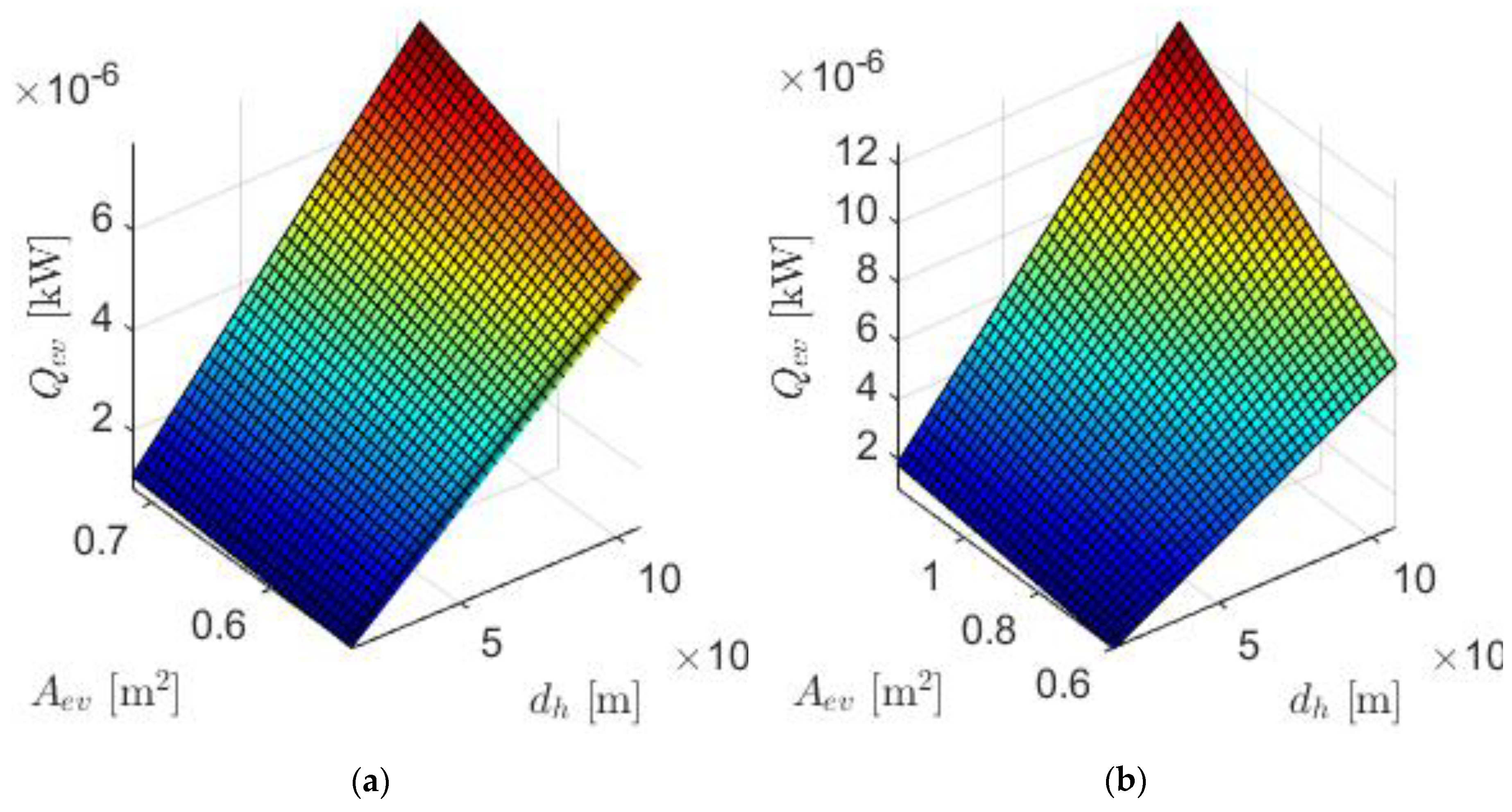
Figure 6.
Exergy efficiency and PBP.
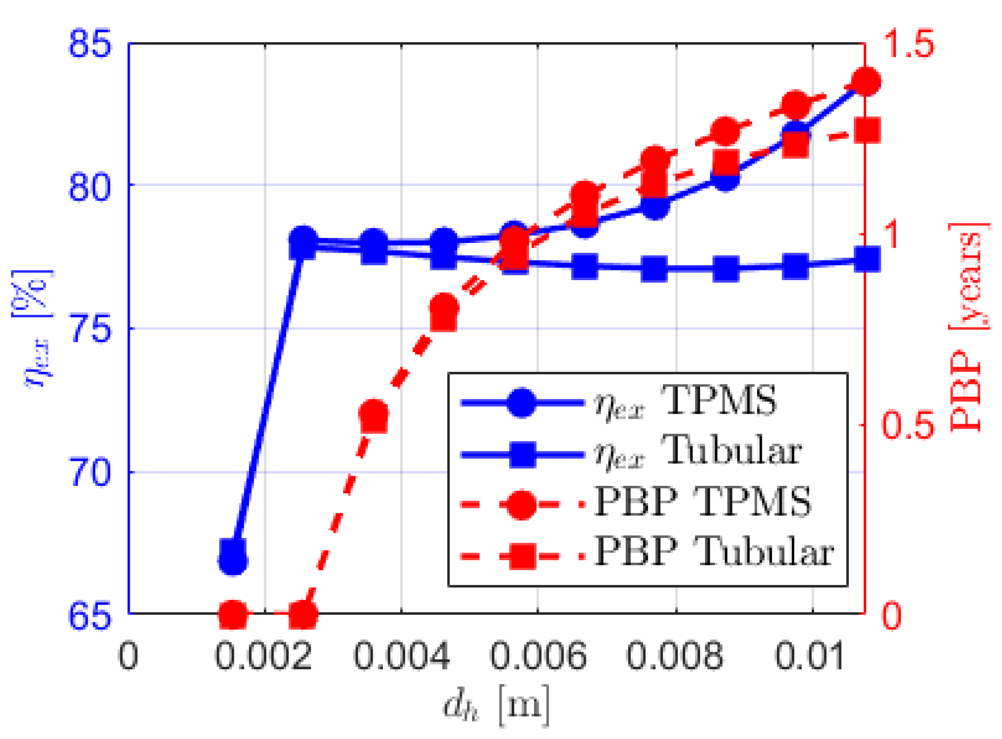
Figure 7.
Equipment investment cost, or Purchase Equipment Cost (PEC).
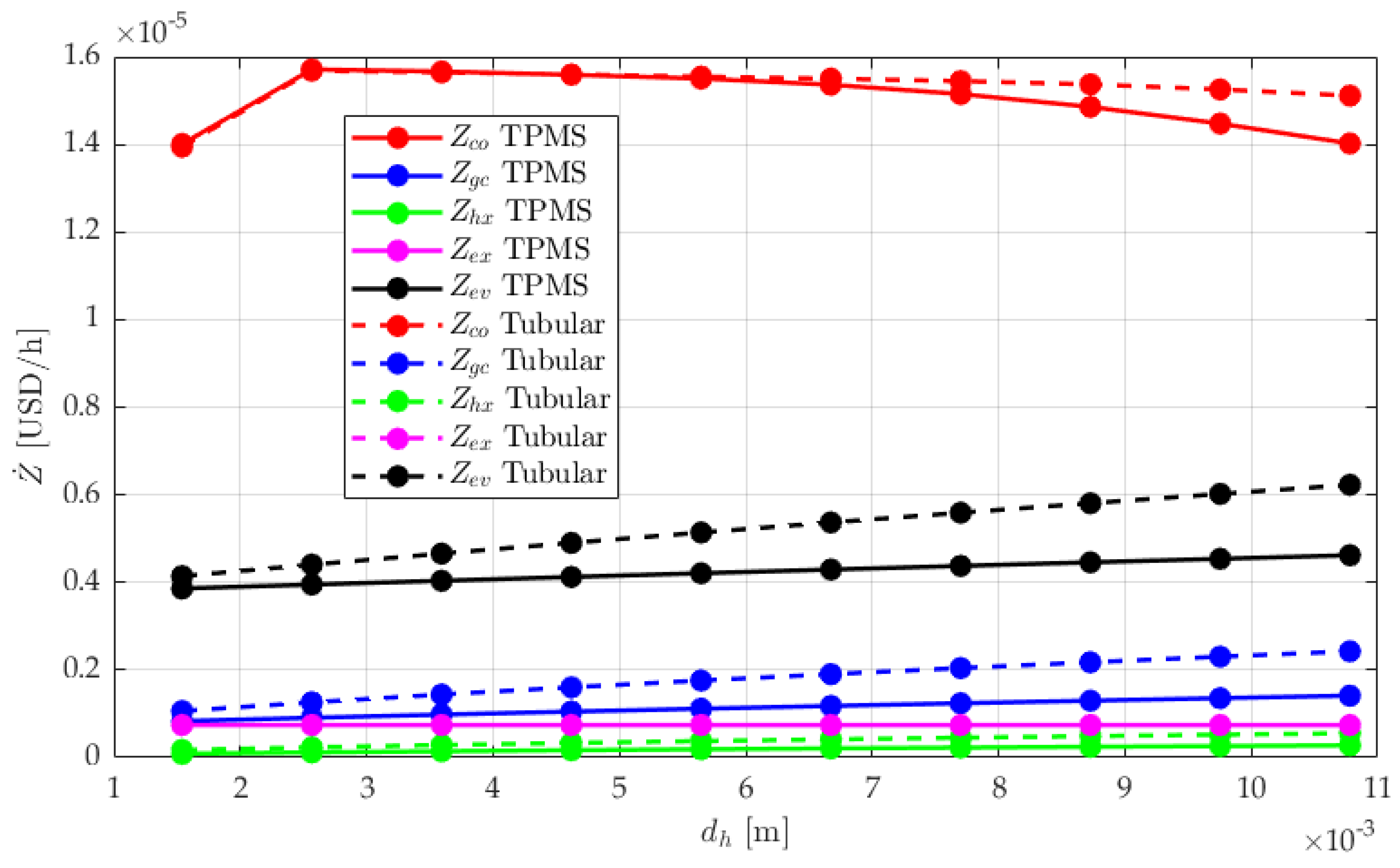
Figure 8.
Exergy cost rate per equipment.
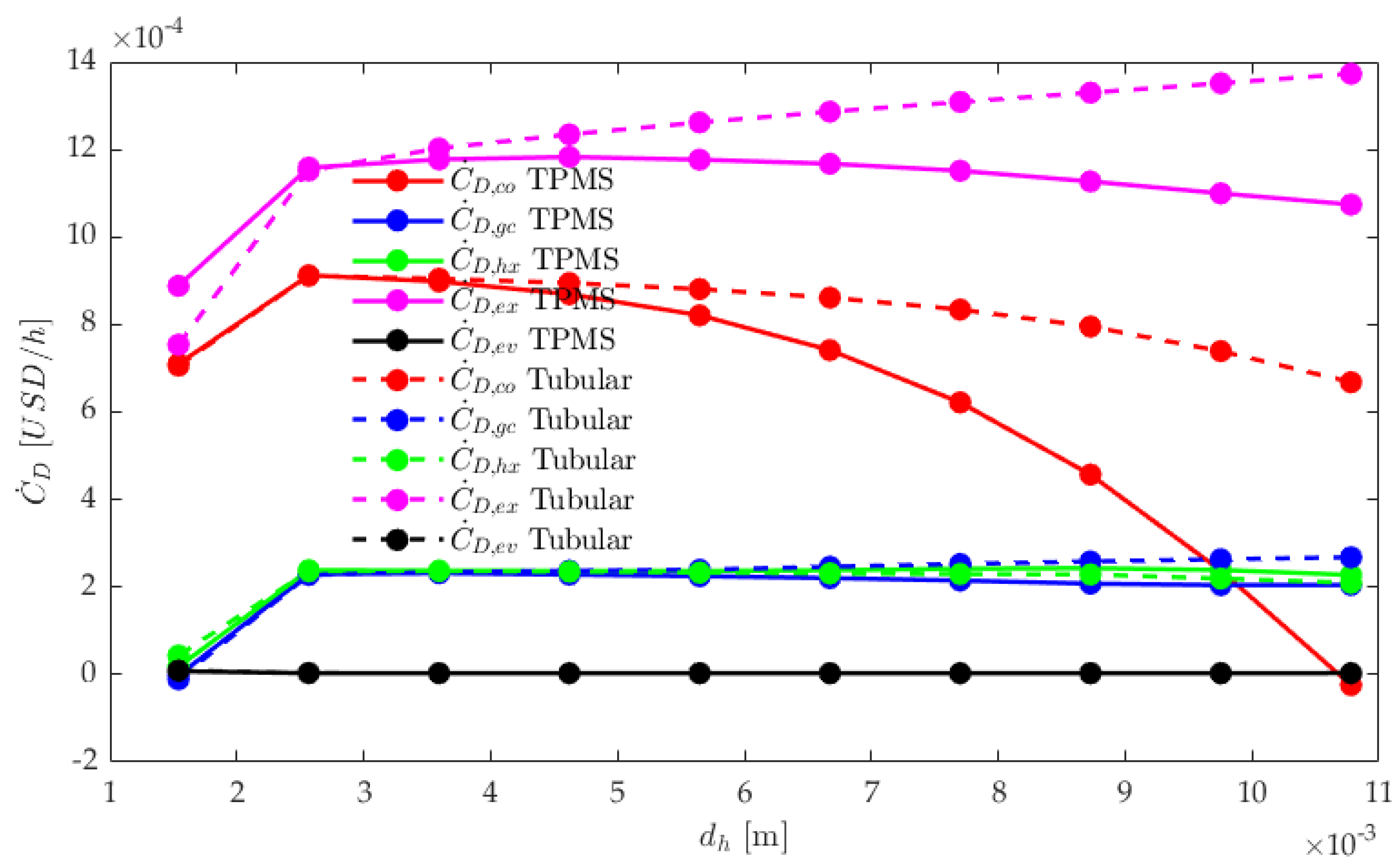
Figure 9.
CO2 penalty cost rate and overall exergy cost rate.
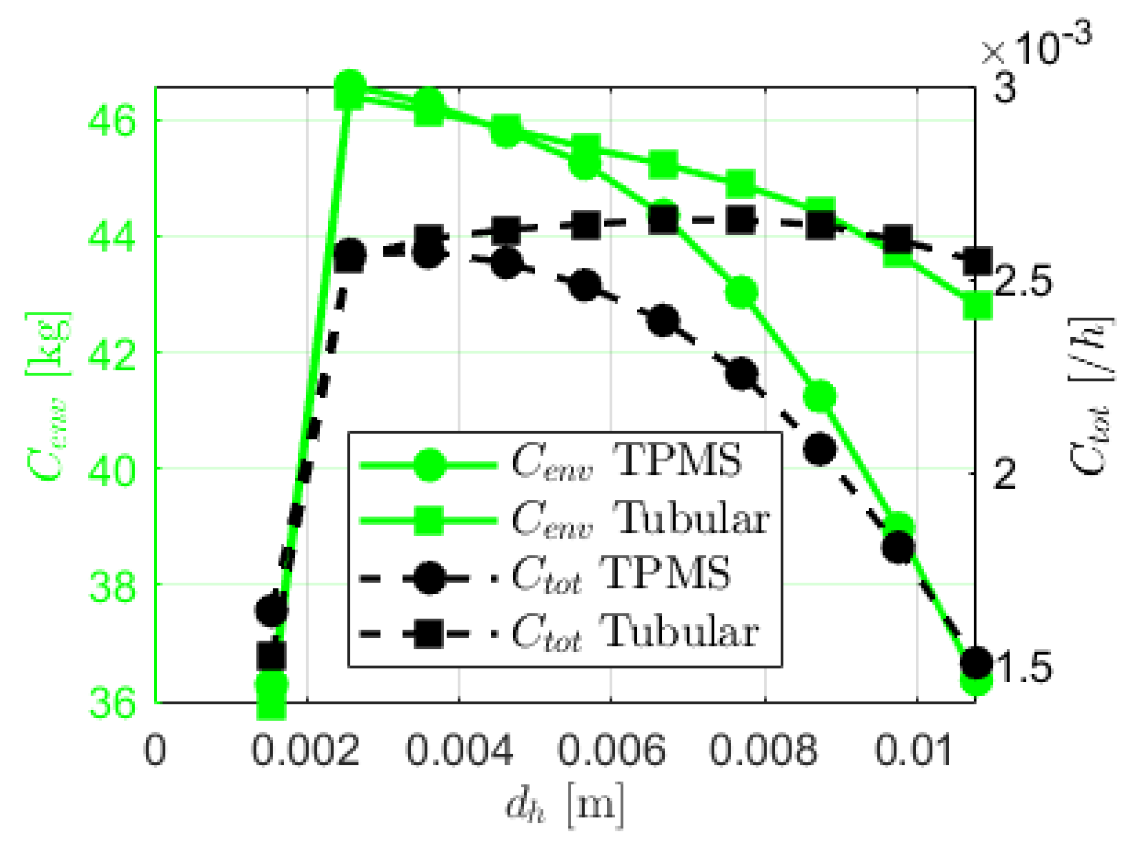
Table 2.
Material properties of AlSi10Mg [28].
Table 2.
Material properties of AlSi10Mg [28].
| Parameter/Material | Symbol | Value | |
|---|---|---|---|
| Material composition balance | Silicon [%] | Si | 9.0 – 11.0 |
| Iron [%] | Fe | 0.55 | |
| Copper [%] | Cu | ≤ 0.05 | |
| Manganese [%] | Mn | ≤ 0.45 | |
| Magnesium [%] | Mg | 0.2 – 0.45 | |
| Nickel [%] | Ni | ≤ 0.05 | |
| Zinc [%] | Zn | ≤ 0.10 | |
| Lead [%] | Pb | ≤ 0.05 | |
| Tin [%] | Sn | ≤ 0.05 | |
| Titanium [%] | Ti | ≤ 0.15 | |
| Thermal properties | Relative density [%] | 99.85 | |
| Material density [g/cm3] | 2.67 | ||
| Wall thermal conductivity [W/(m.K)] | 119 | ||
| Wall specific heat capacity [J/kg/K] | 910 | ||
| Surface roughness [m] | 10e 6 | ||
| Yield strength [MPa] | 240 | ||
| Modulus of elasticity [GPa] | E | 70 | |
| Hardness [HBW] | HR | 119 | |
| Tensile strength [MPa] | 460 |
Table 3.
Structural parameters of the hybrid TPMS heat exchanger.
| Parameter | Symbol | Tubular | TPMS | Source |
|---|---|---|---|---|
| Unit cell length /m | - | [3.0, 5.0, 7.0, 9.0, 11.0, 13.0, 15.0, 17.0, 19.0, 21.0] x e-03 | ||
| to relationship | : | - | [23] | |
| Hydraulic diameter /m | [2.57, 3.59, 4.62, 5.65, 6.67, 7.70, 8.73, 9.75, 10.78, 11.81] x e-03 | |||
| Cross section area /m2 | [23] | |||
| Surface area /m2 | [23] | |||
| Darcy Friction factor | f | |||
| Nusselt number | Nu. | 3.66 | ||
| Where; and for this study are given in Appendix A Table A1 | ||||
Table 4.
Operating parameters and initial conditions.
| Components | Parameter | Symbol | Value |
|---|---|---|---|
| Compartment | Width /m | 1 | |
| Depth /m | 1 | ||
| Height /m | 2 | ||
| Foam thickness /m | 0.05 | ||
| Foam thermal conductivity /W/(m.K) | 0.03 | ||
| Foam heat capacity /J/kJ/K | 1500 | ||
| Foam density /kg/m3 | 30 | ||
| Area of food contents /m2 | 0.25 | ||
| Food density /kg/m3 | 1000 | ||
| Food heat capacity /J/kJ/K | 4000 | ||
| Food volume /m3 | 0.004 | ||
| Compressor | Isentropic efficiency /% | 85 | |
| Cross sectional area /m2 | |||
| Rotational speed /RPM and xMFR /kg/s | acontrolled | ||
| Expansion valve | Discharge coefficient | 0.64 | |
| Pressure ratio | 0.999 | ||
| Restriction area /m2 | bcontrolled | ||
| Evaporator, 1Gas cooler and 2IHX | Evap. conv. heat transfer coef. /W/(m2.K) | 50 | |
| Length of evaporator /m | 20 | ||
| Length of IHX both sides /m | 1 | ||
| Fin thickness /m | 1e-03 | ||
| Hydraulic diameter /m | in Table 3 | ||
| Unit cell length /m | in Table 3 | ||
| Cross sectional area /m2 | in Table 3 | ||
| Area of the fin /m2 | 0.5 | ||
| Area of evaporator /m2 | in Table 3 | ||
| Friction factor | 3.5973 | ||
| Nusselt no. | 27.64337 | ||
| Aggregate eq. length resistance | |||
| Initial conditions | Evaporator: Pressure () = 3.5MPa, Temperature () = 276.15K, Vapor quality (x_init,ev) = 3[0.4, 0.52, 0.64, 0.76, 0.88] Gas cooler: = 10MPa, /K= 4[364, 348, 332, 316, 300], /K=364 IHX hot side: = 10MPa, = 300K, = 300K IHX cold side: = 3.5MPa, x_init,IHXcold = 1 |
||
xMass flow rate, a,bSee the control strategy section, 1The gas cooler and the, 2IHX will bear the subscripts gc and IHX respectively. The 20m length of the 3evaporator and the 4gas cooler is divided into 5 sections, each with its own initial conditions, because Simulink will not simulate the whole length.
Table 5.
Energy and exergy equations.
| Components | Energy balance | * | |||
|---|---|---|---|---|---|
| Compressor | |||||
| Gas cooler | For all; | ||||
| IHX | |||||
| Expansion valve | |||||
| Evaporator | |||||
*general form of exergy equation.
Table 6.
Equipment investment cost and exergy cost rate models.
| Equipment | PECk [Source] |
Reference values | Exergy cost rate bal. equation | Unit exergy cost |
|---|---|---|---|---|
| Compressor |
[31Flors] |
|
|
|
| Gas cooler |
[37] |
|
|
|
| Internal HX |
[37] |
|
|
|
| Expansion valve |
[33] |
|
||
| Evaporator |
[37] |
|
|
|
|
[38] [38] |
||||
Table 7.
Energy comparison between the TPMS-IHX system and the tube based IHX system at 0.01078m.
| Index | Tube HX cycle | TPMS HX-cycle | |
|---|---|---|---|
| Evaluation indices | Wnet /kW | 0.561 | 0.477 |
| Qev /kW | 0.0952 | 0.1063 | |
| ηex /% | 77.39 | 83.62 | |
| Ctot /USD/h | 0.0025 | 0.0015 | |
| PBP /yr | 1.27 | 1.39 | |
| /kg | 42.82 | 36.38 |
Disclaimer/Publisher’s Note: The statements, opinions and data contained in all publications are solely those of the individual author(s) and contributor(s) and not of MDPI and/or the editor(s). MDPI and/or the editor(s) disclaim responsibility for any injury to people or property resulting from any ideas, methods, instructions or products referred to in the content. |
© 2025 by the authors. Licensee MDPI, Basel, Switzerland. This article is an open access article distributed under the terms and conditions of the Creative Commons Attribution (CC BY) license (http://creativecommons.org/licenses/by/4.0/).
Copyright: This open access article is published under a Creative Commons CC BY 4.0 license, which permit the free download, distribution, and reuse, provided that the author and preprint are cited in any reuse.


