
Submitted:
04 June 2025
Posted:
04 June 2025
You are already at the latest version
Abstract
Digital Twin (DT) technology has become a cornerstone of data-driven decision-making in the construction industry through its simulation and predictive capabilities. The integration of Building Information Modeling (BIM) and DT forms a closed-loop system that delivers dynamic operational insights, including predictive maintenance, performance tracking, and risk assessment. This study introduces a BIM-enabled DT framework designed to optimize in-situ production and stockyard management of precast concrete (PC) components. Utilizing the Oracle Crystal Ball simulation tool, probabilistic scheduling and CO₂ emissions optimization were conducted. Results showed potential reductions exceeding 10% in project duration and up to 8.7% in environmental impact. The framework was validated through application to a large-scale logistics warehouse project, providing practical insights for sustainable construction planning.
Keywords:
digital twin
; building information modeling
; precast concrete
; scheduling
; environmental impact
1. Introduction
The construction industry is undergoing a paradigm shift, driven by the emergence of digital technologies that enable the management of complexity, uncertainty, and sustainability [1,2]. As projects grow more intricate with diverse stakeholders, sustainability imperatives, and unpredictable site conditions, digital transformation has become essential. Among these advancements, Digital Twin (DT) technology stands out as a pivotal tool, enabling the real-time synchronization of physical assets with virtual models to support simulation-driven and predictive decision-making [3,4].
The integration of DT with Building Information Modeling (BIM) has garnered increasing attention. BIM provides a foundational platform for data-driven project coordination, design management, and stakeholder collaboration [5,6,7,8,9]. While BIM offers a comprehensive static representation of a facility, DT augments this by incorporating real-time data streams to enable dynamic responses, such as anomaly detection, maintenance forecasting, and risk evaluation, within a closed-loop feedback system [10,11].
Despite these technological advances, significant research gaps remain, particularly in applying BIM-DT integration to optimize the production and storage of precast concrete (PC) components. Prior research has often focused on modular production systems or factory-based simulation models, which tend to lack the flexibility required for resource-constrained, site-specific scenarios [12,13].
Moreover, existing studies have largely overlooked real-time planning for in-situ production and yard layout of PC components [16,17,18,19]. Efficient management of these components demands precise coordination of production, transportation, and temporary storage, all of which are susceptible to spatial limitations, scheduling conflicts, and environmental considerations [20,21]. A comprehensive and real-time platform is urgently needed to monitor, predict, and optimize these tasks.
In particular, studies on in-situ PC production have primarily focused on production area and layout planning [22,23,24,25,26]. However, yard-stock areas are reported to require more than five times the space of production areas [27,28,29,30], and inefficient stockyard layouts can lead to material congestion, schedule delays, and increased environmental burden [31,32,33]. Nonetheless, research on operational strategies and layout management for storage areas remains limited [34,35].
In-situ production replicates the processes of factory manufacturing, rebar placement, formwork, concrete pouring, curing, and temporary storage, on the construction site [36,37,38,39]. This method has been shown to reduce environmental loads by over 14.58% and construction costs by up to 39.4% compared to factory production, without sacrificing quality [24,25,40]. These benefits highlight the need for intelligent, real-time scheduling and layout planning using BIM-integrated DT systems and simulation tools.
Studies also show that in-situ production can yield quality levels equal to or exceeding those of in-plant production, making it competitive in terms of convenience, quality, cost, and schedule [25,26,27,28,29,30,31,32,33,34,35,36,37,38,39,40]. To gain these advantages, it is essential to optimize real-time production and layout planning based on site conditions, requiring the integration of BIM-based DT technology and probabilistic simulation tools. Accordingly, this study proposes a BIM-based digital twin framework designed to optimize the in-situ production and yard-stock layout of PC components. The objectives are to minimize construction duration and carbon emissions through predictive modeling and simulation.
This paper emphasizes the importance of an integrated platform that simultaneously addresses layout efficiency and carbon reduction strategies as a key enabler for sustainable construction. And simulation tools such as Oracle Crystal Ball are applied. The scope of this study is confined to steel-reinforced concrete (SRC) precast components.
The research follows these steps:
- 1)
- Analyze each stage of in-situ PC production and stockyard management
- 2)
- Review BIM and DT applications in the construction industry
- 3)
- Analyze time requirements for each production stage
- 4)
- Simulate integrated production and yard management using BIM for a real logistics center project
- 5)
- Optimize the construction schedule using Crystal Ball based on BIM data
- 6)
- Optimize CO₂ emissions using the same simulation approach
- 7)
- Compare layout scenarios to validate the effectiveness of the proposed framework
2. Literature Review
2.1. Integration of BIM and DT in the Construction Industry
BIM has become a foundational platform for construction information management, supporting tasks such as design coordination, scheduling, and resource allocation [10,35]. However, BIM traditionally functions as a static system, lacking the ability to reflect real-time conditions on site. To address this limitation, DT technology is increasingly being adopted to create dynamic, real-time representations of physical environments [3,4].
The integration of BIM and DT has significantly improved decision-making across the project lifecycle by enhancing visualization, operational control, and performance monitoring. For instance, Opoku et al. (2021) utilized DT to improve site visibility and adaptive decision-making [41], while Kassem et al. (2022) applied IoT-based DT frameworks for real-time equipment tracking [42]. Other studies, such as those by Xu et al. (2024) have reviewed the technical challenges and strategic benefits of integrating digital technologies in construction [43].
Importantly, recent research has expanded DT applications to include environmental impact assessment through Life Cycle Assessment (LCA). Chen et al. (2021) [44], Tagliabue et al. (2023) [45] and Alizadehsalehi et al. (2021) [46] demonstrate how DT can be linked to LCA metrics to promote low-carbon construction and compliance with environmental regulations.
Lu et al. (2020) further illustrated the value of integrating sensor data into BIM-DT systems to enable anomaly detection in facility monitoring [11]. Opoku et al. (2021) emphasized the use of real-time data from IoT and machine learning models to enhance the predictive capabilities of DT [41]. According to Xu et al. (2024), the transition from BIM to DT represents a fundamental evolution in construction workflows, one that enables system-wide intelligence and predictive control [43].
2.2. DT for Predictive Planning and Risk Management
DT’s core strength lies in its ability to simulate future scenarios and support proactive decision-making in complex environments. For example, Lu et al. (2020) developed a DT-based approach to improve coordination and productivity in on-site construction processes[11]. Zhang et al. (2024) applied DT for real-time environmental monitoring and integrated lifecycle carbon footprint analysis into planning workflows [47].
More recently, scenario-based and probabilistic simulation tools have been embedded within DT frameworks. Bakhshi et al. (2024) introduced a DT platform that incorporates simulation techniques for proactive risk mitigation and emission tracking [48]. The integration of optimization algorithms with DT has proven especially useful in improving the responsiveness and reliability of construction project control systems.
2.3. On-Site Precast Concrete Production and Stockyard Management
Effective management of in-situ production and temporary storage is critical in precast construction, where just-in-time assembly and spatial optimization are essential. Kosse et al. (2020) proposed a simulation-based model for optimizing yard layout in precast construction [49], while Lim and Kim (2024) explored the integration of scheduling and spatial constraints in PC logistics planning [25].
However, many existing models remain static and are not responsive to real-time conditions. To overcome this limitation, it is essential to incorporate sensor inputs and intelligent simulation platforms within DT systems. Environmental optimization is an area that has not yet been adequately addressed in the literature.
2.4. Simulation-Based Optimization of Schedule and Environmental Impact
The integration of simulation tools, such as Oracle Crystal Ball, within BIM-DT systems enables the evaluation of multiple planning scenarios under uncertainty. Monte Carlo simulation is effective for modeling probabilistic outcomes related to schedule variation and emission profiles. Nikoukar and Tavakolan (2025) demonstrated the potential of such techniques to improve logistics planning, project resilience, and sustainability outcomes [50].
While traditional tools like Primavera and MS Project generate deterministic schedules, tools like Crystal Ball allow for probabilistic risk assessment. When combined with BIM and DT, this enables simultaneous optimization across various dimensions, including productivity, safety, and environmental performance.
2.5. Research Gap
Despite growing interest in DT applications, there remains a lack of fully integrated BIM-DT systems specifically tailored to the complexities of precast concrete logistics. In particular, few frameworks support simulation-based optimization of CO₂ emissions in tandem with production and yard management. This study aims to address this gap by proposing a unified platform that enables real-time synchronization, predictive simulation, and environmentally conscious decision-making for in-situ PC component production.
3. Case Application of BIM-Based In-Situ Production
3.1. Selection of the Case Project
To validate the effectiveness and practical applicability of the proposed BIM-based digital twin framework, a real-world construction project was selected as a case study. The project involves the construction of a large-scale logistics warehouse located in A City. The structure consists of four above-ground floors, with precast concrete (PC) slabs installed from Level 1 to Level 4. The building’s core structure is composed of reinforced concrete (RC), and the ramp areas utilize a combination of steel and steel-reinforced concrete (SRC) systems. This study focuses primarily on the PC slab construction processes across the four floors.
3.2. Analysis of In-Situ Production and Installation Time for PC Components
To identify risks and inefficiencies in in-situ PC production, the entire process—from formwork to installation—was thoroughly analyzed. The PC construction process comprises three main stages: production, transportation (minimal in this case), and installation. Due to the large spans and high ceiling requirements of the warehouse, the components used are oversized, requiring specialized handling.
Production begins with mold preparation, including cleaning, assembly, installation of embedded items, and rebar placement. Following this, a release agent is applied, concrete is cast and compacted, and the components undergo steam curing before demolding. Post-curing activities involve hoisting, surface finishing, inspection, and temporary yard storage.
Installation starts with site preparation and crane connection, followed by component hoisting, positioning, temporary jointing, and alignment verification. Cranes are allocated based on mold availability and construction schedules, and idle cranes are dynamically reassigned to support in-situ production. The time required for each sub-process was estimated and compiled, as shown in Table 1.
The number of required molds is calculated based on production quantity, production cycle, and total production duration. Similarly, the number of cranes is determined by the unit erection time, total installation quantity, and allowable erection period. The total yard area is estimated by multiplying the number of stored components by the unit yard area per component type. These calculations are formalized in Equations (1) through (3).
where, Nm: number of molds; QMi: in-situ production quantity of each mold type; TPC: production cycle time; Ts: in-situ production time; i: number of mold types (1, … , n).
where, NC : number of cranes; ; TUE: unit erection time QS : in-situ production quantity; Te: erection time
where, AYS: yard stock area, QYSi: yard stock quantity of each mold type, AUYSi: unit yard stock area of each mold type, i :number of mold types(1, … , n))
1) Comparison Between In-Plant and In-Situ Production
PC production for large-scale projects typically follows one of two methods: in-plant or in-situ. In the in-plant method, production occurs at a centralized facility, involving material preparation, mold assembly, rebar installation, and embedding. After casting and curing, components are temporarily stored until they reach the required strength for delivery and installation.
In contrast, in-situ production eliminates the need for long-distance transportation, allowing components to be fabricated and installed on-site. This approach is particularly advantageous in spatially constrained projects, as it reduces handling and logistics risks. However, crane operation times become a critical factor in overall project scheduling. If yard space is limited, production must be closely aligned with the installation plan to minimize on-site storage. In some cases, hybrid approaches combining partial in-plant production may be adopted to address spatial constraints.
Given the nature of the case project, with oversized components and restricted yard space, it was assumed that components would be installed immediately after production, minimizing the need for intermediate storage.
2) Installation Process of PC Components
Installation of PC components is carried out using crawler cranes, chosen for their superior lifting capacity and mobility relative to tower cranes. The process includes preparing for lifting, attaching components to lifting equipment, vertical hoisting, transportation to the installation location, and final placement.
After hoisting, vertical and horizontal members are positioned, followed by rebar integration, joint treatment, and curing. These stages are highly interdependent, requiring integrated management across production, temporary storage, and installation workflows (Najafi et al., 2015). Proper synchronization is essential to avoid delays and ensure structural quality.
3) Process-Based Work Time Estimation
To estimate the overall construction duration, work times for each process stage were analyzed based on field knowledge and prior literature (Lim et al., 2017a). This included production sub-tasks such as rebar placement and casting, as well as installation and transportation tasks. Labor requirements and durations for each sub-task were estimated using practical experience and domain knowledge (Lim et al., 2017a).
The analysis revealed that the full production cycle requires approximately 985 minutes (16.42 hours), while the installation cycle takes about 32 minutes per component. The installation time, although not directly applied in the simulation model, informs crane operation planning and resource allocation.
3.3. Analysis of Yard Layout Planning for In-Situ Produced PC Components
The yard layout process follows the sequence of production, storage, and installation [24,25,51]. As illustrated in Figure 1 (a), components are first produced based on zone-specific requirements identified from design drawings. Since component shapes and sizes vary, multiple mold types are required. Zones are classified by component type (e.g., beams, columns, slabs), and production is planned to meet the earliest possible installation deadline within each zone. As production, storage, and installation quantities are the same, the components to be installed are identified. The quantity is calculated to determine the target quantity for in-situ production. The location of the column and beam components for each zone of in-situ production quantity is analyzed through design drawing analysis.
The number of members and area for yard-stock of Figure 1(b) are calculated. And the required yard-stock area is calculated by multiplying the number of members. The production and yard storage available area for each process are calculated, and the yard storage and production arrangement plan are simulated based on the reviewed area. If yard storage and production are not satisfied, the arrangement simulation is completed through repeated modifications (feedback routine). For yard storage simulation, first, the crane movement path is analyzed and the possibility of utilizing the yard space is reviewed. At this time, the yard space is determined by dividing it into before and during the installation of PC members. The yard-stock utilization order is determined, the possibility of utilizing the yard-stock space according to the in-situ production schedule is reviewed.
For PC component installation, as shown in Figure 1(c), the number of cranes required is determined based on the in-situ production duration. The specifications of each crane, such as work radius and lifting capacity, are defined accordingly [52]. Based on the number of cranes, zoning plans are established. The zoning plan is established based on the number of cranes. Installation sequence is determined, and installation time is estimated for each component type (columns, beams, slabs). Finally, the installation schedule is simulated according to the construction schedule. In other word, in-situ produced PC components are first arranged in the storage yard and installed in sequence.
3.4. 4D Simulation Using BIM
For efficient in-situ production and yard layout, implementation of digital twins using BIM and optimal space planning strategies based on time series analysis are required. These values were established based on actual site conditions during the preparation stage for in-situ production. The assumption conditions of the main factors for BIM implementation are as shown in Table 2. This is a value that was reflected considering the on-site conditions during the on-site production preparation stage. The required construction period presented by the client is 18 months, and the applied quantity is 1,035ea of columns and 1,906ea of beams. The in-situ production cycle using form (mold) is 2 days and the lead time is 5 months. Lead-time refers to the period from M+1 to M+5 during which only PC members are produced. In other words, only in-situ production and yard storage are performed during this period, and PC members are not installed.
And the number of molds applied is 32ea for columns and 90ea for beams. Two cranes were assigned, corresponding to the number of designated work zones. The maximum yard storage area derived by reflecting these conditions was calculated to be 13,235㎡. The construction period applied on site was estimated to be 8 months within the range of compliance with the client's requested construction time (18 months). According to Lim et al. (2020) [53], the number of mold cycles makes a profit when 39 PC parts are produced with one mold. If the mold is not sufficient, the lead-time requires a considerably long period, so this study applied 40-50 times.
The production and yard-stock areas for a unit area are calculated as shown in the table. The following equations (4) and (5) were applied for the area. The production area, installation area, and yard-stock area for one member are 16.5㎡ and 9.6㎡, respectively. The maximum yard-stock area of 15,235㎡ was derived at lead-time M+5. The reason why the highest number of yard-stock members is shown during this period is because the PC members produced during the lead-time were accumulated. And since the yard-stock members are installed, the number of PC members decreases as they are installed. The period from M+6 to M+8 means time-lag and is 3 months. That is, when construction begins, the yard-stock area gradually increases, and the largest yard-stock area is recorded just before the start of installation (M+6). And when installation begins, the yard-stock area decreases, and when the area becomes 0, the PC construction is finished.

Table 3.
Monthly area (unit: 1,000㎡).
| Monthly area | 1 | 2 | 3 | 4 | 5 | 6 | 7 | 8 |
| Production area | 12.1 | 12.1 | 12.1 | 12.1 | 12.1 | 0.0 | 0.0 | 0.0 |
| Yard stock area | 2.8 | 5.7 | 8.5 | 11.3 | 13.9 | 8.2 | 4.1 | 0.0 |
Ap(t) = 1∑n{Ai | t ∈ [Si, Ei)}
Ay(t) = 1∑n{Ai | t ∈ [Si, Ii)}
Ap(t): In-situ production area occupied at time t, Ay(t): Yard-stock area occupied at time t, Si: Production start date of the ith component, Ei: Production completion date of the ith component, Ii: Installation date of the ith component
Figure 2 shows the 4D simulation after the installation of PC members has started, built using BIM. PC members are not installed during the lead time from M+1 to M+5. Therefore, only the construction from M+6 to M+8 is shown. In M+6, the production areas of zone A and zone B are 630㎡ and 580㎡, respectively, and the yard-stock areas of zone A and zone B are 7,124㎡ and 6,812㎡, respectively. In the case of a general in-situ production system, since the erection area is added, it is difficult to produce and store PC members in the same location, so the production and yard-stock locations can have to be moved. However, in this study, only the production location was moved, and the yard-stock location was set up to be the closest location to the installation location.
4. Optimization of Schedule and CO₂ Emission
Lim et al. (2020) [52] explained six assumptions about the available area selected as the main influencing factor, and derived the highest cost reduction rate among the scenarios applicable to the field. In addition, Lim et al. (2020) [40] derived Min and Max for each factor such as in-situ production quantity, lead time, number of molds, and number of cranes, and analyzed the effect of quantity on cost and CO₂. However, this study assumes that all members are produced, and derives factors affecting the process and CO₂ emission. In addition, the goal was to reduce environmental loads by 10% within the range where the construction time can be reduced by more than 10%.
4.1. Schedule Optimization
This study proposes an in-situ production and construction schedule optimization method of PC members using the Oracle Crystal Ball simulation tool based on member quantity information extracted from BIM data. At construction sites, the accuracy and reliability of schedule planning can easily be reduced due to the variability of material quantity, inter-task dependency, and unexpected delay factors. To solve this, this study quantifies the process risk according to quantity change through Monte Carlo simulation based on probabilistic variables, analyzes the sensitivity, and derives the optimal scenario. The objective function used for construction duration optimization is defined as follow Equation (6).
Tt: Total duration of in-situ production, Tpi: Production time of the ith component, Tyi: Yard storage and transportation time of the ith component, Tei: Installation time of the ith component, n: Total number of components
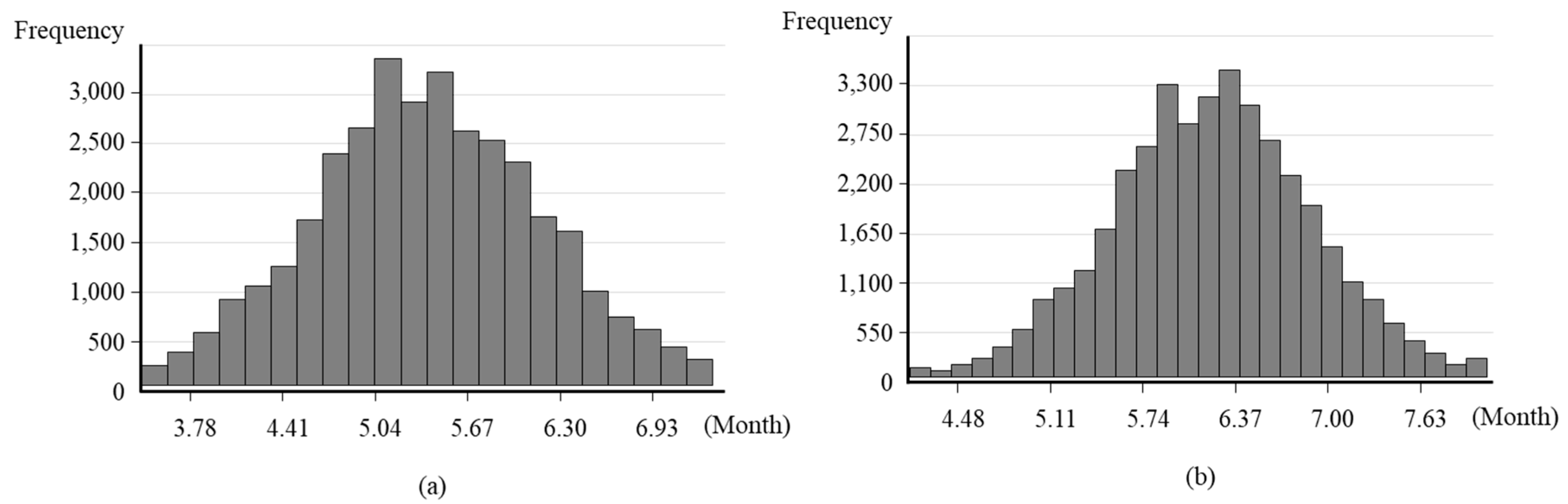
The schedule optimization was performed through the maximum repetition simulation (1,000,000 times) in the Oracle Crystal Ball program. The simulation results were derived using the normal distribution. All possible cases of lead time and construction period were derived, and Min and Max for each factor were derived. The factors used as parameters at this time were quantity, production cycle, lead time, number of molds, and number of cranes. Assuming that the construction period is within the allowable range, it was considered to be within 18 months considering the construction period requested by the client. As a result of deriving the Min-Max management range of lead time as shown in the following figure, Min was set to 3.53 months and Max to 7.28 months. The reason why the lead time does not decrease below 3.53 months is because only PC members whose production is complete can be installed, so it is necessary to secure the members production period. The construction time was estimated as Min 14.11 months and Max 17.99 months.
Figure 3.
Control range of lead-time and construction time: (a) Lead-time; (b) Construction time.
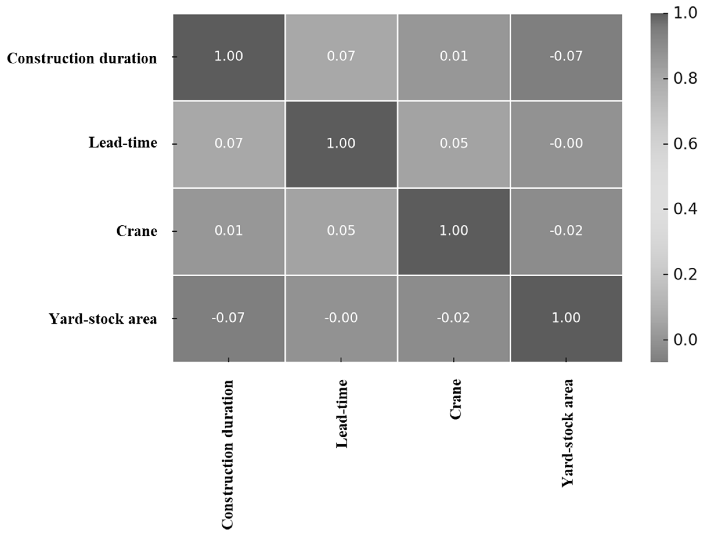
Lead-time and duration were analyzed to have a correlation coefficient of +0.59, which means that the total construction period increases when the lead time increases. Duration and yard-stock area had a correlation coefficient of -0.52, which means that as the construction period gets longer, the mold is used to produce PC members in a timely manner, which reduces the yard-stock area. In addition, lead-time and yard-stock area had a correlation coefficient of +0.18, which means that the yard-stock area also increases somewhat when the lead time increases. In addition, cranes and the remaining variables showed a relatively weak correlation, which means that the number of cranes did not have a significant effect on the construction period and yard-stock area. This is because the total installation period is short, so the crane has a relatively small effect on the total construction period compared to other variables. For the algorithms for the process of deriving the final optimal value, refer to appendix 1. The work time for each stage is analyzed, and the number of forms considering the yard-stock area is derived. Then, the lead time and total construction period applied with the number of forms are derived, and the yard-stock area is calculated.
Figure 4.
Sensitivity Analysis.
Using the management ranges of lead time and construction time derived through Monte Carlo simulation, the optimal case is derived as shown in Table 4. The construction time is derived as 6.3 months, which is the smallest value among the values that can be shortened by more than 10% of the applied construction period of 8 months. In addition, this represents a 75% reduction compared to the client’s original 18-month construction schedule. The number of molds is 22 columns, 60 beams, the lead time is 4.8 months, and the number of cranes is 2. The yard-stock area is derived as 12,342㎡. Through these results, the minimum value can be derived in terms of the construction period, and it can be seen that the lead time corresponding to this value is not the smallest value. In addition, the appropriate construction time can be derived by considering various factors in the future and applied to the site, and various decision-making related to the process plan can be supported.
4.2. CO₂ emission Optimization
Based on the quantity data extracted from the BIM model, this study presents a procedure for quantifying and optimizing CO₂ emissions generated during the production and yard storage of PC components using Oracle Crystal Ball. Carbon emissions at construction sites vary sensitively depending on the distance traveled by materials, equipment operation time, yard density, and work waiting time. However, this study focuses on the main factors of in-situ production. CO₂ emissions are calculated using actual labor inputs, along with oil and electricity consumption during the production and storage processes. The objective function for CO₂ emission optimization, as well as the CO₂ emission calculation formulas, are provided in Equations (7)–(9).
: total CO₂ emission, : CO₂ emission of column, : CO₂ emission of beam, : ith column quantity, : unit CO₂ emission of labor, : unit CO₂ emission of oil, : unit CO₂ emission of electricity, : unit CO₂ emission of lighting and heating, : unit CO₂ emission of environmental conservation, : ith beam quantity, : Number of installed ith column (1, … , n), : Number of installed ith beam (1, … , m)
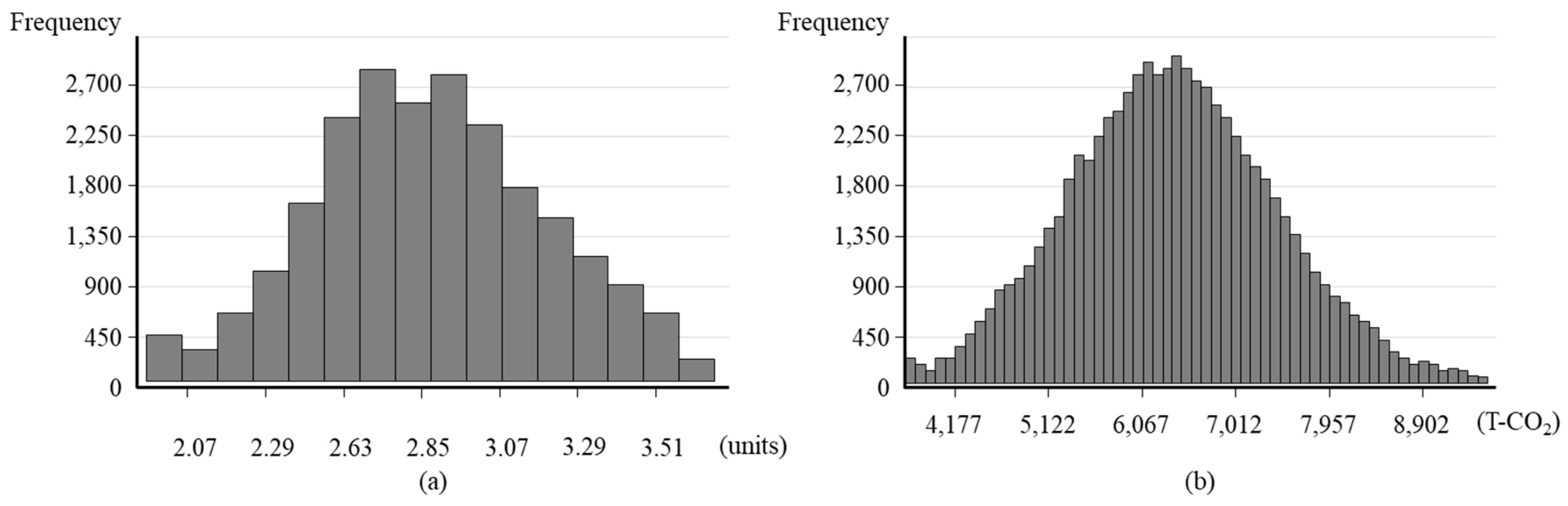
In the same way as schedule optimization, CO₂ emission optimization was performed through maximum repetition simulation (1,000,000 times) in the Oracle Crystal Ball program. All possible cases of crane and CO₂ occurrence were derived to derive Min and Max for each factor. The factors used as parameters at this time were quantity, production cycle, lead-time, number of molds, and number of cranes. As a result of deriving the Min-Max management range of the crane as shown in the following figure, Min was set to 2.00 ea and Max was set to 3.270 ea. The reason why the crane does not decrease below 2.00 months is because the minimum number of cranes is required to match the process. And CO₂ emission was estimated as Min 35,352 T- CO₂ and Max 97,244 T-CO₂. As a result of analyzing the management range, the crane and CO₂ emission according to the change in each factor were generally proportional, so they appeared in a graph of a similar shape.
Figure 5.
Control range of crane and CO₂ emission: (a) Crane; (b) CO₂ emission.
Using the management scope of crane and CO₂ emission derived through Monte Carlo simulation, the optimal case is derived as shown in Table 5. CO₂ emission is derived as 40,423 T- CO₂, construction time is 6.5 months, and this value is the smallest value among the derived CO₂ emission values. The number of molds is 30 columns, 91 beams, lead time is 5.1 months, number of cranes is 2, and yard-stock area is 15,729㎡. Through the results, it is analyzed that CO₂ emission increases as the number of cranes increases, which means that the crane is a factor that increases CO₂ emission. In the future, the values of various factors can be determined on site considering the minimum CO₂ emission by considering various factors. For the algorithms for the process of deriving the final selected optimal CO₂ emission, refer to Appendix 2. The number of forms according to the yard-stock area is derived, and the lead time and total construction period applied to the number of forms are derived, and the yard-stock area is calculated. CO₂ emissions were calculated by applying these results step by step.
5. Conclusion
This study proposed a BIM-based digital twin framework to optimize in-situ production, yard-stock management, and installation of PC components in large-scale construction projects. By integrating probabilistic simulation with BIM-derived data, the framework effectively addressed the core constraints of time, space, and environmental impact within a unified digital environment.
Using Oracle Crystal Ball, the study conducted Monte Carlo simulations to evaluate construction schedule risks and CO₂ emissions. The schedule optimization revealed a strong correlation between lead-time and project duration, underscoring the importance of production planning in meeting construction deadlines. Conversely, crane quantity showed minimal impact on overall duration, given the relatively short installation phases.
The optimal construction duration identified was 6.3 months, exceeding the project’s target of a 10% reduction compared to the original 8-month schedule. This is 75% shorter than the client’s required construction duration. CO₂ emissions were optimized to 40,423 T-CO₂, with a construction time of 6.5 months, highlighting the significant environmental benefits achievable through intelligent layout and production planning. Notably, increased crane use was associated with higher carbon output, indicating that equipment operation is a key driver of environmental load.
Overall, the results validate the feasibility of predictive and simulation-driven planning in managing complex construction variables. By enabling real-time synchronization of production, yard layout, and installation processes, the proposed framework contributes to more sustainable and resilient construction strategies.
From an academic perspective, this research advances the application of DT in construction by holistically integrating time, spatial layout, and environmental performance into a single model. Practically, it provides actionable insights for project managers and policy makers seeking to implement smart, low-carbon construction practices. However, the findings are limited to a single case project and do not yet incorporate real-time sensor feedback or automated 3D yard modeling.
Future research should focus on expanding the applicability of the framework by:
- Integrating real-time sensor data for dynamic feedback control,
- Applying machine learning techniques to improve CO₂ emission forecasting,
- Enhancing safety and risk management through predictive analytics, and
- Developing cloud-based visualization dashboards for intelligent site monitoring.
By addressing these directions, the framework can evolve into a fully autonomous, adaptive Digital Twin system capable of supporting the next generation of sustainable construction management.
Author Contributions
Conceptualization, S.K. and J.L.; methodology, J.L.; software, J.P. and J.L.; validation, J.L.; formal analysis, J.P. and J.L.; investigation, S.K. and J.L.; resources, J.P., S.K. and J.L.; data curation, J.P. and J.L.; writing—original draft preparation, J.P. and J.L.; writing—review and editing, J.P., S.K. and J.L.; visualization, J.L.; supervision, S.K. and J.L.; project administration, S.K. and J.L.; funding acquisition, S.K. and J.L. All authors have read and agreed to the published version of the manuscript.
Funding
This work was supported by the National Research Foundation of Korea (NRF) grant funded by the Korea government (MOE) (No. 2021R1C1C2094527 and No. 2022R1A2C2005276).
Data Availability Statement
The raw data supporting the conclusions of this article will be made available by the authors on request.
Conflicts of Interest
The authors declare no conflicts of interest.
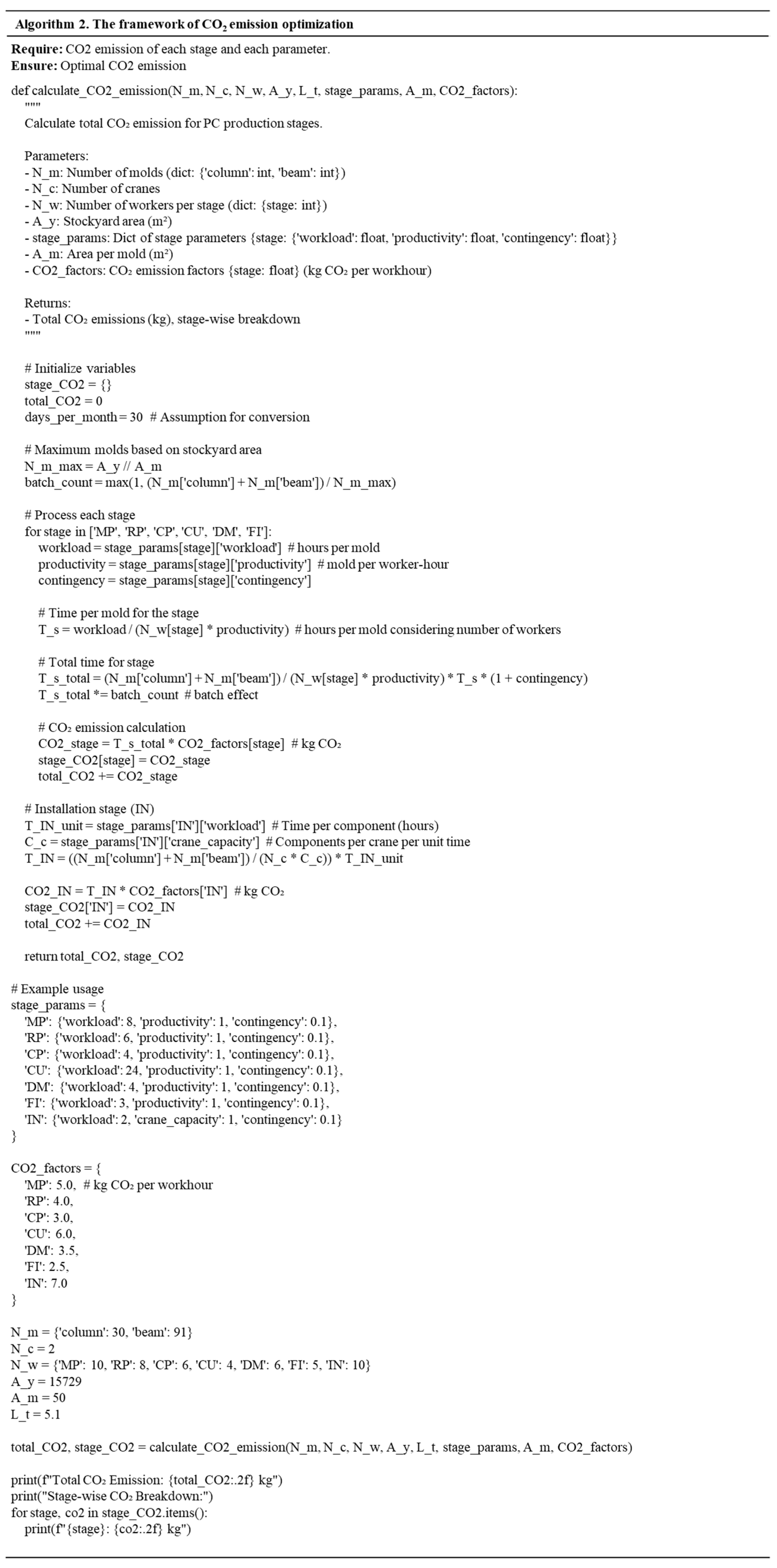
Appendix A
Figure A1.
Algorithms for the process of deriving the selected optimal schedule.
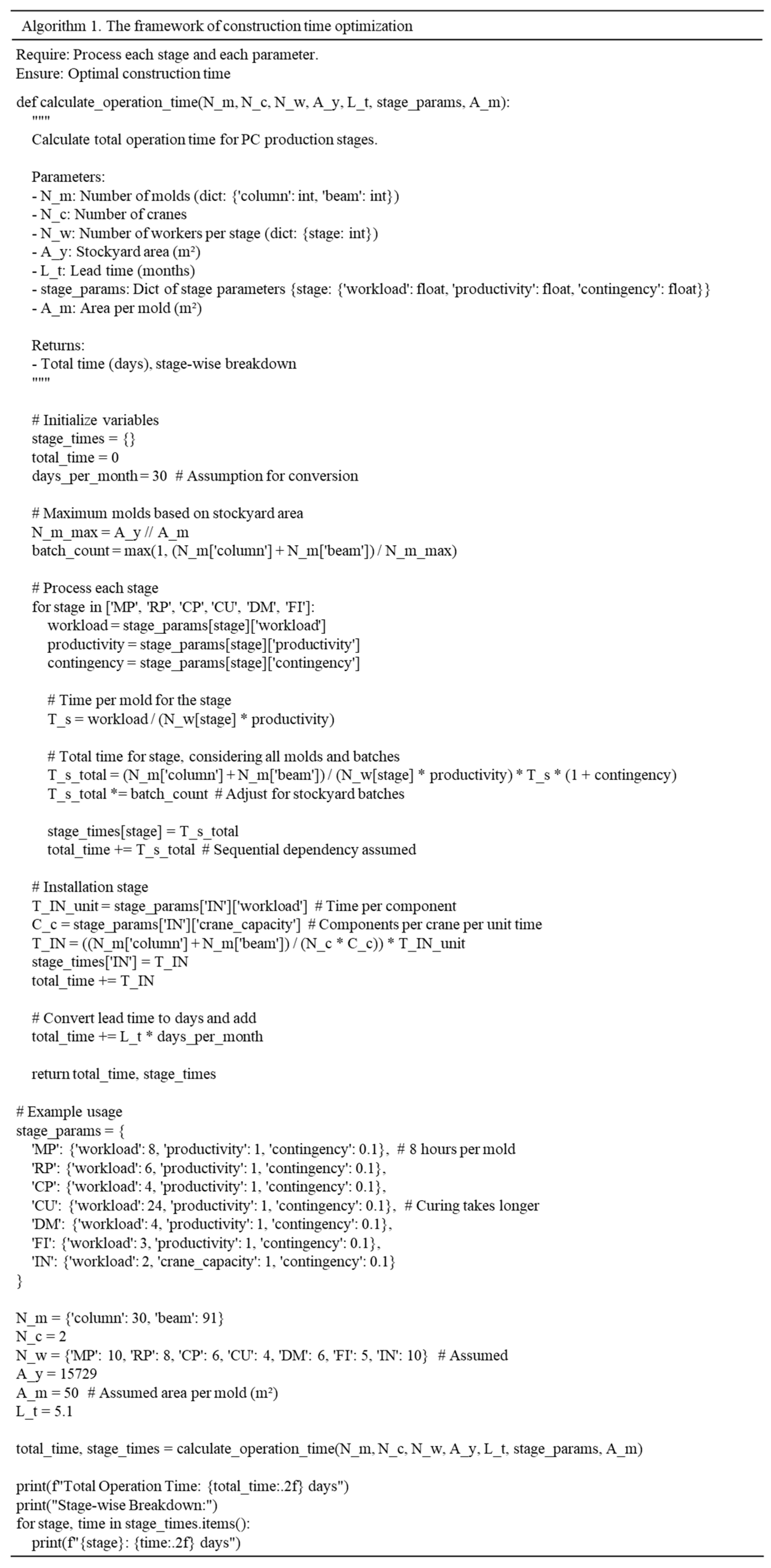
Figure A2.
Algorithms for the process of deriving the selected optimal CO₂ emission.
References
- Merschbrock, C., & Munkvold, B. E. (2024). The digital transformation of the construction industry: A review. Industrial and Commercial Training, 56(2), 123–140. [CrossRef]
- Nyqvist, R., Peltokorpi, A., Lavikka, R., & Ainamo, A. (2025). Building the digital age: management of digital transformation in the construction industry. Construction Management and Economics, 43(4), 262-283. [CrossRef]
- Qi, Q., & Tao, F. (2021). Digital twins and big data towards smart manufacturing and Industry 4.0: 360-degree comparison. Advanced Engineering Informatics, 59, 101542. [CrossRef]
- Boje, C., Guerriero, A., Kubicki, S., & Rezgui, Y. (2020). Towards a semantic construction digital twin: Directions for future research. Automation in Construction, 114, 103179. [CrossRef]
- Jeong, S.-H., & Kim, G.-H. (2024). Development of BIM Utilization Level Evaluation Model in Construction Management Company. Korean Journal of Construction Engineering and Management, 25(4), 24–33. [CrossRef]
- Hwang, J., Song, S. H., Lee, C., Ahn, H., Cho, H., & Kang, K.-I. (2024). BIM and OpenAI-based Model for Supporting Initial Construction Planning of Bridges and Tunnels. Korean Journal of Construction Engineering and Management, 25(6), 24–33. [CrossRef]
- Kang, H., & Seong, H. (2025). Conceptual Model for Quality Risk Assessment and Reserve Cost Estimation for Construction Projects based on BIM. Korean Journal of Construction Engineering and Management, 26(2), 62–71. [CrossRef]
- Kim, H., & Nam, J. (2025). Applying BIM Standard Guideline to Expressway BIM Results and Drawing its Improvement Measure for Project Management. Korean Journal of Construction Engineering and Management, 26(2), 82–88. [CrossRef]
- Kim, I., & Shah, S. H. (2025). A Proposal for Evaluation Criteria of Decision Support System for BIM. Korean Journal of Construction Engineering and Management, 26(2), 89–102. [CrossRef]
- Sacks, R., Brilakis, I., Pikas, E., Xie, H. S., & Girolami, M. (2020). Construction with digital twin information systems. Data-Centric Engineering, 1, e14. [CrossRef]
- Lu, Q., Parlikad, A. K., Woodall, P., Ranasinghe, G. D., Xie, Y., Liang, Z., & Konstantinou, E. (2020). Developing a digital twin at building and city levels: Case study of West Cambridge campus. Journal of Management in Engineering, 36(3), 05020004. [CrossRef]
- Jiang, Y., Li, M., Guo, D., Wu, W., Zhong, R. Y., & Huang, G. Q. (2022). Digital twin-enabled smart modular integrated construction system for on-site assembly. Computers in Industry, 136, 103594. [CrossRef]
- Guo, J., Zhao, N., Sun, L. et al. Modular based flexible digital twin for factory design. J Ambient Intell Human Comput 10, 1189–1200 (2019). [CrossRef]
- Al-Kahwati, K., Birk, W., Nilsfors, E. F., & Nilsen, R. (2022, June). Experiences of a digital twin based predictive maintenance solution for belt conveyor systems. In PHM Society European Conference (Vol. 7, No. 1, pp. 1-8). [CrossRef]
- Chen, Z., Tan, Y., & Zhang, A. (2023). Integrating digital twin and blockchain for smart building management. Sustainable Cities and Society, 99, 104514. [CrossRef]
- Lim, C.; Joo, J.K.; Lee, G.J.; Kim, S.K. Basic Analysis for Form System of In-situ Production of Precast Concrete Members. In Proceedings of the 2011 Autumn Annual Conference of Construction Engineering and Management, Seoul, Republic of Korea, 27–30 October 2011; Volume 12, pp. 137–138. [Google Scholar]
- Lim, C.-Y.; Joo, J.-K.; Lee, G.-J.; Kim, S.-K. In-situ Production Analysis of Composite Precast Concrete Members of Green Frame. J. Korea Inst. Build. Constr. 2011, 11, 501–514. [Google Scholar] [CrossRef]
- Lee, G.J.; Lee, S.H.; Joo, J.K.; Kim, S.K. A Basic Study of In-Situ Production Process of PC Members. In Proceeding of the 2011 Autumn Annual Conference of the Architectural Institute of Korea, 2011 Oct 28-29, Seoul, Republic of Korea, 2011; Volume 31, pp. 263–264. [Google Scholar]
- Lee, G.J.; Joo, J.K.; Lee, S.H.; Kim, S.K. A Basic Study on the Arrangement of In-situ Production Module of the Composite PC Members. In Proceeding of the 2011 Autumn Annual Conference of the Korea Institute of Building Construction, Seoul, Republic of Korea, 2011 Oct 28-29, Seoul, Republic of Korea, 2011; Volume 11,pp. 29–30.
- Lim, J.; Kim, J.J. Dynamic optimization model for estimating in-situ production quantity of PC members to minimize environmental loads. Sustainability 2020, 12, 8202. [Google Scholar] [CrossRef]
- Hong, W.-K.; Lee, G.; Lee, S.; Kim, S. Algorithms for in-situ production layout of composite precast concrete members. Autom. Constr. 2014, 41, 50–59. [Google Scholar] [CrossRef]
- Na, Y.J.; Kim, S.K. A process for the efficient in-situ production of precast concrete members. J. Reg. Assoc. Archit. Inst. Korea 2017, 19, 153–161. [Google Scholar]
- Lim, C. Construction Planning Model for In-situ Production and Installation of Composite Precast Concrete Frame. Ph.D. Thesis, Kyung Hee University, Seoul, Republic of Korea, 2016. [Google Scholar]
- Lim, J.; Son, C.-B.; Kim, S. Scenario-based 4D dynamic simulation model for in-situ production and yard stock of precast concrete members. J. Asian Arch. Build. Eng. 2022, 22, 2320–2334. [Google Scholar] [CrossRef]
- Lim, J., & Kim, S. (2024). Environmental Impact Minimization Model for Storage Yard of In-Situ Produced PC Components: Comparison of Dung Beetle Algorithm and Improved Dung Beetle Algorithm. Buildings, 14(12), 3753. [CrossRef]
- Jung, H.T.; Lee, M.S. A Study on the Site-production Possibility of the Prefabricated PC Components. In Proceeding of the 1992 Autumn Annual Conference of the Architectural Institute of Korea, Seoul, Republic of Korea, 1992 Oct 24, Seoul, Republic of Korea, 1992; Volume 12, pp. 629–636.
- Li, H.; Love, P.E. Genetic search for solving construction site-level unequal-area facility layout problems. Autom. Constr. 2000, 9, 217–226. [Google Scholar] [CrossRef]
- Won, I.; Na, Y.; Kim, J.T.; Kim, S. Energy-efficient algorithms of the steam curing for the in situ production of precast concrete members. Energy Build. 2013, 64, 275–284. [Google Scholar] [CrossRef]
- Kim, S.; Kim, G.; Kang, K. A Study on the effective inventory management by optimizing lot size in building construction. J. Korea Inst. Build. Constr. 2004, 4, 73–80. [Google Scholar] [CrossRef]
- Lee, J.M.; Yu, J.H.; Kim, C.D. A Economic Order Quantity (EOQ) Determination Method considering Stock Yard Size; Korea Institute of Construction Engineering and Management, , Seoul, Republic of Korea: 2007; pp. 549–552.
- Lee, J.M.; Yu, J.H.; Kim, C.D.; Lee, K.J.; Lim, B.S. Order Point Determination Method considering Materials Demand Variation of Construction Site. J. Archit. Inst. Korea 2008, 24, 117–125. [Google Scholar]
- Thomas, H.R.; Horman, M.J.; Minchin, R.E.; Chen, D. Improving labor flow reliability for better productivity as lean construction principle. J. Constr. Eng. Manag. 2003, 129, 251–261. [Google Scholar] [CrossRef]
- Yun, J.-S.; Yu, J.-H.; Kim, C.-D. Economic Order Quantity(EOQ) Determination Process for Construction Material considering Demand Variation and Stockyard Availability. Korean J. Constr. Eng. Manag. 2011, 12, 33–42. [Google Scholar] [CrossRef]
- Dobson, D. W., Sourani, A., Sertyesilisik, B., & Tunstall, A. (2013). Sustainable construction: analysis of its costs and benefits. American Journal of Civil Engineering and Architecture, 1(2), 32-38.
- Volk, R., Stengel, J., & Schultmann, F. (2014). Building Information Modeling (BIM) for existing buildings—Literature review and future needs. Automation in Construction, 38, 109–127. [CrossRef]
- Osman, H.M.; Georgy, M.E.; Ibrahim, M.E. A hybrid CAD-based construction site layout planning system using genetic algorithms. Autom. Constr. 2003, 12, 749–764. [Google Scholar] [CrossRef]
- Ning, X.; Lam, K.-C.; Lam, M.C.-K. Dynamic construction site layout planning using max-min ant system. Autom. Constr. 2009, 19, 55–65. [Google Scholar] [CrossRef]
- Abdul-Rahman, H.; Wang, C.; Eng, K.S. Repertory grid technique in the development of Tacit-based Decision Support System (TDSS) for sustainable site layout planning. Autom. Constr. 2011, 20, 818–829. [Google Scholar] [CrossRef]
- Lee, G.J. A Study of In-situ Production Management Model of Composite Precast Concrete Members. Ph.D. Thesis, Kyung Hee University, Seoul, Republic of Korea, 2012. [Google Scholar]
- Lim, J.; Kim, S. Evaluation of CO2 Emission Reduction Effect Using In-situ Production of Precast Concrete Components. J. Asian Arch. Build. Eng. 2020, 19, 176–186. [Google Scholar] [CrossRef]
- Opoku, D. G. J., Perera, S., & Osei-Kyei, R. (2021). "Digital Twins for the Built Environment: Learning from Conceptual and Process Models in Manufacturing." Smart and Sustainable Built Environment, 10(4), 557–575.
- Kassem, M., Kelly, G., Dawood, N., Serginson, M., & Lockley, S. (2015). "BIM in Facilities Management Applications: A Case Study of a Large University Complex." Built Environment Project and Asset Management, 5(3), 261–277.
- Xu, Q., Wang, J., Gao, W., Ren, S., & Li, Z. (2024, October). Digital Twin: State-of-the-Art and Future Perspectives. In Proceeding of the 2024 5th International Conference on Computer Science and Management Technology (pp. 731-740).
- Chen, C., Zhao, Z., Xiao, J., & Tiong, R. (2021). A conceptual framework for estimating building embodied carbon based on digital twin technology and life cycle assessment. Sustainability, 13(24), 13875.
- Tagliabue, L. C., Brazzalle, T. F., Rinaldi, S., & Dotelli, G. (2023). Cognitive Digital Twin Framework for Life Cycle Assessment Supporting Building Sustainability. In Cognitive Digital Twins for Smart Lifecycle Management of Built Environment and Infrastructure (pp. 177-205). CRC Press.
- Alizadehsalehi, S., Hadavi, A., & Huang, J. C. (2021). "From BIM to Extended Reality in AEC Industry." Journal of Information Technology in Construction (ITcon), 26, 1–17.
- Zhang, Z., Wei, Z., Court, S., Yang, L., Wang, S., Thirunavukarasu, A., & Zhao, Y. (2024). A review of digital twin technologies for enhanced sustainability in the construction industry. Buildings, 14(4), 1113. [CrossRef]
- Bakhshi, S., Ghaffarianhoseini, A., Ghaffarianhoseini, A., Najafi, M., Rahimian, F., Park, C., & Lee, D. (2024). Digital twin applications for overcoming construction supply chain challenges. Automation in Construction, 167, 105679. [CrossRef]
- Kosse, S., Forman, P., Stindt, J., Hoppe, J., König, M., & Mark, P. (2023, June). Industry 4.0 enabled modular precast concrete components: a case study. In International RILEM Conference on Synergising expertise towards sustainability and robustness of CBMs and concrete structures (pp. 229-240). Cham: Springer Nature Switzerland.
- Nikoukar, S., & Tavakolan, M. (2025). A simulation-based approach to optimizing resource allocation and logistics in construction projects: a case study. Engineering, Construction and Architectural Management.
- Na, Y.J.; Kim, S.K. A process for the efficient in-situ production of precast concrete members. J. Reg. Assoc. Archit. Inst. Korea 2017, 19, 153–161. [Google Scholar]
- Lim, J.; Kim, S.; Kim, J.J. Dynamic simulation model for estimating in-situ production quantity of pc members. Int. J. Civ. Eng. 2020, 18, 935–950. [Google Scholar] [CrossRef]
- Lim, J.; Park, K.; Son, S.; Kim, S. Cost reduction effects of in-situ PC production for heavily loaded long-span buildings. J. Asian Arch. Build. Eng. 2020, 19, 242–253. [Google Scholar] [CrossRef]
Figure 1.
Production-stock yard-erection process of PC components: (a) In-situ production; (b) Yard-stock; (c) Erection.
Figure 1.
Production-stock yard-erection process of PC components: (a) In-situ production; (b) Yard-stock; (c) Erection.
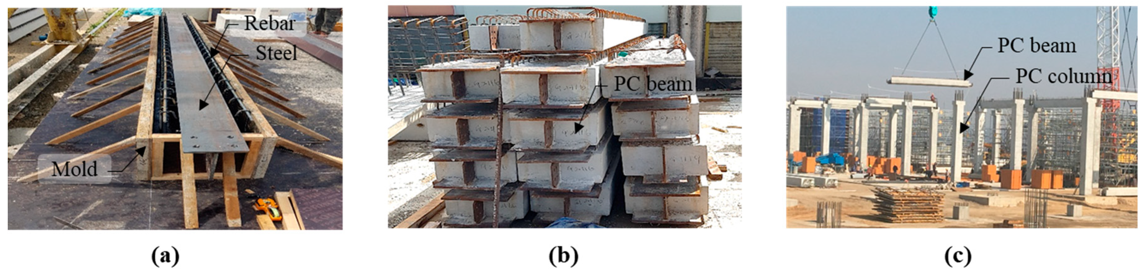
Figure 2.
Monthly site plan using BIM: (a) D+12; (b) D+24; (c) D+36; (d) D+48.
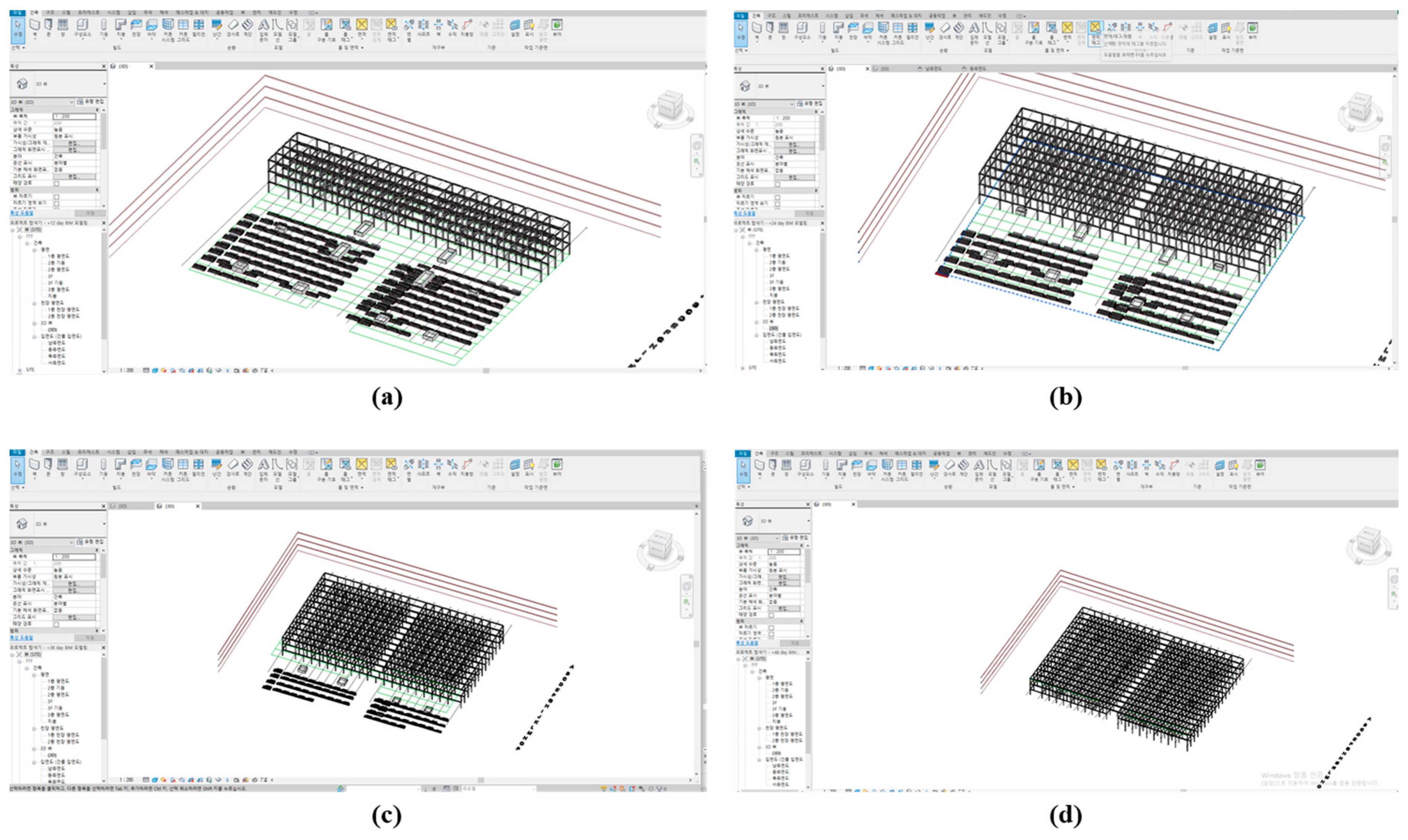
Table 1.
Analysis of work time in in-situ production.
| Work | Process | Required labor | Work Time (min) |
|---|---|---|---|
| Form work | Mold installation | Two common labors | 2 |
| Cleaning | Two common labors | 2 | |
| Stirrup support installation | Two common labors | 1 | |
| Rebar and insert installation | Four common labors | 50 | |
| Concrete work | Release mold agent application | Two common labors | 2 |
| Concrete casting and compaction | Four common labors | 20 | |
| Surface finishing | Two common labors | 5 | |
| Curing work | Curing sheet installation | Two common labors | 720 |
| Steam curing | Two common labors | ||
| Demolding | One common labors | 10 | |
| Yard-Stock work | Yard-stock preparation | Two common labors | 2 |
| Hoisting | Two common labors | 6 | |
| Dismantling binding | One common labors | 5 | |
| Inspection | Each one of skilled and common labor | 60 | |
| Plastering | Each one of skilled and common labor | 100 | |
| PC installation | Lifting preparation and component binding | Two common labors | 2 |
| Lifting | Two common labors | 6 | |
| Alignment | Two common labors | 19 | |
| Final binding removal | One common labors | 5 |
Table 2.
Assumed conditions for BIM implementation.
| Category | Details | |
| Required Construction Duration (month) | 18 | |
| Applied construction Duration (month) | 8 | |
| Quantity (ea) | Column | 1,035 |
| Beam | 1,906 | |
| Production Cycle (day) | 2 | |
| Number of Molds (ea) | Column | 32 |
| Beam | 90 | |
| Lead-time (month) | 5 | |
| Number of Cranes (ea) | 3 | |
| Maximum yard stock area (㎡) | 15,235 m2 | |
Table 4.
Optimization Result for schedule.
| Item | unit | Value | |
| Construction time | month | 6.3 | |
| Number of molds | Column | ea | 22 |
| Beam | ea | 60 | |
| Lead-time | Months | 4.8 | |
| Cranes | ea | 3 | |
| Yard-stock area | ㎡ | 12,342 | |
Table 5.
Optimization Result for schedule.
| Item | unit | Value | |
| CO₂ emission | T-CO₂ | 40,423 | |
| Construction time | month | 6.5 | |
| Number of molds | Column | ea | 30 |
| Beam | ea | 91 | |
| Lead-time | Months | 5.1 | |
| Cranes | ea | 3 | |
| Yard-stock area | ㎡ | 15,729 | |
Disclaimer/Publisher’s Note: The statements, opinions and data contained in all publications are solely those of the individual author(s) and contributor(s) and not of MDPI and/or the editor(s). MDPI and/or the editor(s) disclaim responsibility for any injury to people or property resulting from any ideas, methods, instructions or products referred to in the content. |
© 2025 by the authors. Licensee MDPI, Basel, Switzerland. This article is an open access article distributed under the terms and conditions of the Creative Commons Attribution (CC BY) license (http://creativecommons.org/licenses/by/4.0/).
Copyright: This open access article is published under a Creative Commons CC BY 4.0 license, which permit the free download, distribution, and reuse, provided that the author and preprint are cited in any reuse.


