
Submitted:
04 June 2025
Posted:
04 June 2025
You are already at the latest version
Abstract
In this paper, the stability and stabilization problems of singular fractional order systems (FOSs) with order α∈(0,1) are investigated. Firstly, admissibility criteria for singular FOSs are proposed by introducing full-column rank matrices. Next, the admissibility criterion using only one (linear matrix inequality) LMI variable is presented. A branch-and-bound algorithm (BBA) is designed to solve the bilinear constraints appearing in the stabilization criterion. Finally, the validity of the given results is verified by numerical simulations.
Keywords:
Singular fractional-order systems
; admissibility criteria
; branch-and-bound algorithm
; full-column rank matrix
; strict LMI
1. Introduction
Fractional-order systems (FOSs) have attracted a wide range of attention in recent years from an application point of view, since many physical systems can be described concisely and accurately in terms of FOSs [1,2]. Thanks to the great efforts of researchers, many valuable results have been obtained for stability analysis [4] and controller synthesis [5] of FOSs.
Stability is a key issue in control theory [6,7,8,9,10], particularly for FOSs. As in the case of integer-order systems (IOSs) [11,12], the stability of linear FOSs [13] depends on the localization of eigenvalues in the complex plane [14]. However, the research results in [14] lack a systematic approach to solving the stability problem of FOSs and are limited to stability analysis rather than control applications. Since the early 1960s, the linear matrix inequalities (LMI) approach has been instrumental in control theory, primarily since many control-related problems can be formulated as convex optimization problems involving LMIs [15]. In terms of stability, one of the most well-known LMI conditions arises from applying Lyapunov theory to linear time-invariant systems of integer order. This LMI condition enables testing whether the system poles are located in the left half of the complex plane. Due to the differing stability domain properties across various fractional-order intervals [16], researchers have classified the order of FOSs into two primary ranges: and . In the study of singular FOSs, the issues are significantly more complex than in standard systems, as the admissibility property—including regularity, non-impulsiveness, and stability—must be addressed. Many challenging problems remain in the area of stability analysis and controller synthesis for singular FOSs. In fact, either the decision matrix involves complex numbers [17,18,19] and too many numbers [20,21], or the criteria yield LMI conditions with equality constraints[22,23]. These limitations make these criteria too complex to be used directly in controller design. For example, [21] makes assumptions about the form of the variables in the controller design, thus introducing conservatism. Furthermore, the results in [24,25] were in the bilinear matrix inequality form, which is more complicated to solve. In order to eliminate these drawbacks, some results have been proposed for the synthesis of state feedback controllers in the form of LMI based on matrix singular value decomposition [26]. However, the results presented in [26] only provide sufficient conditions. For singular FOSs of order belonging to ,27,28] provided design methods for state feedback controllers and state output feedback controllers, respectively. Nevertheless, [27,28] focused only on the stability problem rather than the broader admissibility problem and provided results under the assumption that singular FOSs are regular, which does not always hold. In recent years, some results using strict LMIs have been reported for solving control problems of various types of FOSs. In [29], the problem of stability and robust stabilization of FOSs is investigated and an approach using strict LMIs with minimal decision variable is proposed. In [30,31,32,33], control methods for singular FOSs are also proposed, including state feedback control, derivative feedback control and control. For , Zhang et al. [34] proposed a unified framework for singular FOSs.
The above discussion motivates us to focus on the issue of admissibility and stabilization of singular FOSs. First, the bilinearity problem encountered in state feedback controller design is solved using the branch-and-bound algorithm (BBA). Subsequently, the extension of the results in [11] gives necessary and sufficient conditions for the admissibility criteria of singular FOSs. Finally, the singular matrix decomposition technique is used for state feedback control of closed-loop systems. The main contributions are summarized as follows:
- (1)
- The proposed admissibility criteria are different from all existing criteria. Unlike in [21], which involves an excessive number of decision variables, the proposed admissibility criterion uses only a single LMI variable. This paper not only reduces computational complexity but also extends the results of [11] from IOSs to singular fractional-order systems with orders in .
- (2)
- These criteria provide several advantageous characterizations of existing results. The proposed approach avoids the use of complex variables [17,18,19], making it well-suited for handling eigenvalues of system matrices with positive real parts; it does not involve a large number of LMI variables [20] and does not contain equality constraints [22,23], making it easy to both for controller design and numerical simulation.
- (3)
- Admissibility and stabilization problems for singular FOSs with orders in the interval solved. Equality constraints and non-strict linear matrix inequalities have been removed in all admissibility conditions to facilitate checking. A BBA was devised to solve the bilinear problem [24,25] arising in stabilization criterion.
The paper is organized as follows: The foundational results needed for the analysis are provided in Section 2. Section 3 details the main findings related to singular FOSs. Section 4 validates these results with computational examples. In conclusion, Section 5 presents final remarks and highlights the main contributions.
Notations : Let denotes that X is a complex matrix of dimension and denotes that X is a real matrix of dimension . denotes a complex number, where and denote the real and imaginary parts of , respectively; denotes the imaginary unit. I denotes the unit matrix with the appropriate dimension. represents that the eigenvalues of the matrix X are all less than zero (greater than zero). The conjugate transpose (transpose) of the matrix X is denoted as and is denoted as . The symbol denotes the Kronecker product of the matrices X and Y. Given a fractional order , let , where and .
2. Problem Statements and Preliminaries
Consider the following singular fractional-order linear system
where denotes the state vector; is the fractional order; and represent the known matrices; signifies a singular matrix with a rank of m, where m is less than n. In case of , system (1) reduces to
For the given system (2), there exist dimensional real invertible matrices G and W satisfying
A sufficient and necessary condition for the system (2) to be impulse-free is that the matrix is non-singular.
The system described in (2) is admissible if and only if the following statements hold, respectively:
- (1)
- for , there exist dimensional real square matrices X and Y such that
- (2)
- for , there exist dimensional real square matrices X and Y, and dimensional real matrix Q, such thatwhere S is an dimensional matrix characterized by full column rank, such that .
The system described in (2) with is asymptotically stable if and only if there exist dimensional real square matrices X and Y satisfying inequality (4) and
Given an complex matrix Z, then the following three inequalities are equivalent:
- (1)
- (2)
- (3)
where the real and imaginary parts of Z are denoted by X and Y, respectively.
3. Main Results
3.1. Novel Admissibility Conditions for Singular FOSs
This section introduces new admissibility criteria based on LMIs.
In case of , the system described in (2) is admissible if and only if there exist dimensional symmetric real matrix P and dimensional anti-symmetric real matrix Q that satisfy the following LMIs
where the definition of S is same as Lemma 2.
(Sufficiency) It is supposed that inequalities (6) and (7) are hold. There exist reversible matrices G and W satisfying inequality (3). Decompose the matrix as
Let
Then, Let
Multiplying the 1-1 block in (6) by on the left side and on the right by its transpose, yields
where * represents the entries that are not relevant in the following discussion. Thus, , i.e., is a non-singular matrix. According to Lemma 1, system (2) is regular and impulses-free. The next step involves demonstrating the stability of system (2). Let be the generalized eigenvalue of system (2) and be the eigenvector corresponding to . Then
By pre-multiplying Eq. (7) by and post-multiplying by its conjugate transpose, the following result is obtained:
For , there are and . System (2) is stable when (with in the case that ); thus, only the case is considered. In this scenario, . Let By applying Lemma 4, inequality (6) is equivalent to
and
Multiplying inequality (12) on the left by and on the right by its conjugate transpose, it yields that
Multiplying inequality (13) on the left by and on the right by its conjugate transpose, results in the following inequality:
Multiplying the 1-1 block in inequality (6) on the left by and on the right by its conjugate transpose, results in the following inequality:
The following discussion is categorized based on the comparison of with zero.
(1) In case of : By the definition of b, it follows that . According to inequalities (11), (14) and (16), there is
witch indicates that , i.e.,
(2) In case of : By the definition of b, it follows that .
If , from inequality (14), inequality
indicates that . Then, according to inequality (15), we have that
which contradicts inequality (11). Thus, this case is not valid.
Therefore, inequality (11) always holds. At this point,
In summary, the fact that the inequalities (17) and (18) hold indicates that condition
holds. Therefore, the system (2) is stable.
(Necessity) Suppose that the system (2) is admissible. According to the property of a block matrix, there exist invertible matrices satisfying the following conditions:
as well as
According to Lemma 3, there exist matrices and that satisfy the inequalities (4) and (5). Set
Then,
From inequalities (4), (5) and (23), inequality (6) holds. Meanwhile,
which shows that inequality (7) holds. □
Theorem 1 extends the admissibility criterion for singular IOSs established in [11] to singular FOSs in the interval using minor LMI variables. For conventional linear systems ( and ), conditions (6) and (7) reduce to the well-known condition that the matrix A is Hurwitz: there exists a matrix such that .
According to Theorem 1, by setting and , an admissibility criterion using only one LMI variable can be obtained.
In case of , the system described in (2) is admissible if and only if there exists dimensional real matrix X that satisfy the following LMIs
where the definition of S is same as Lemma 2.
Corollary 1 is derived from a strict LMI-based criterion that eliminates the need for equality constraints and avoids the introduction of redundant decision variables. This simplification enhances computational efficiency and leads to more practical and fundamental results.
While Theorem 1 provides necessary and sufficient conditions for determining the acceptability of the system (2), it suffers from the disadvantage that it involves bilinear matrix inequalities, which complicates the design of the controller. The following result addresses this limitation by introducing a matrix Q that linearizes the nonlinear term associated with A in Theorem 1.
In case of , the system described in (2) is admissible if and only if there exist dimensional symmetric real matrix P, dimensional anti-symmetric real matrix Q and dimensional real matrix H that satisfy the following LMIs
where the definition of S is same as Lemma 2.
(Sufficiency) There exist reversible matrices G and W satisfying inequality (3). Then, the 1-1 block in (26) becomes
where * represents the entries that are not relevant in the following discussion; G and S satisfied (8) and (9); . Thus, is a non-singular matrix, i.e., is a non-singular matrix. According to Lemma 1, system (2) is regular and impulses-free. Subsequently, from the stability analysis presented in the sufficiency proof of Theorem 1, it follows that the satisfaction of inequalities (26) and (27) establishes the stability of the system. Thus, the system (2) is proved to be admissible since it is regular, impulse-free, and stable.
(Necessity) Assuming the system (2) is admissible. Based on Theorem 1, it follows that inequalities (6) and (7) hold. Let
Then inequalities (26) and (26) hold. □
For and , one obtains for Theorems 1 and 2. In this case, the LMIs conditions given in Theorems 1 and 2 all reduce to the LMIs conditions provided in Lemma 3. For , the singular FOSs reduces to the singular IOSs. Thus, these results extend Lyapunov stability theorem from the normal IOSs to the singular FOSs of order .
3.2. Novel Stabilization Conditions for Singular FOSs
Consider the state feedback controller given by
Applying the controller in (29) to system (1) yields the following closed-loop singular FOS:
Consider the system (31)
Since systems (2) and (31) have the same generalized eigenvalues, system (2) is admissible if and only if system (31) is admissible. Therefore, Theorems 1 and 2 remain valid by simultaneously taking and satisfying .
Considering the closed-loop singular FOS (30) and applying Theorem 2 in conjunction with Remark 5, the desired results are obtained immediately.
For the system described in (2), the existence of the state feedback controller 29 makes the closed-loop system 30 admissible if and only if there exist dimensional symmetric real matrices P, dimensional antisymmetric real matrices Q and dimensional real matrix H that satisfies
where the definition of S is same as Lemma 2.
In Theorem 3, the feedback gain K is coupled to and , respectively. This means that Theorem 3 contains bilinear terms, it cannot be solved directly using the LMI toolbox. Therefore, a Branch and Bound Algorithm (BBA) is employed to determine the control system parameters and K, subject to the conditions of LMIs (32) and (33). First, the variables M and N are introduced to linearize the bilinear term in Eqs. (32) and (33), yielding relaxation LMIs (34) and (35).
Then, solving LMIs (34) and (35) yields the initial values of and N. Afterwards, the initial value of K is obtained via Eq. (36).
Since the required feasible solutions and K need to satisfy the equations (32) and (33), only the inequalities (37), (38) and (39) need to be considered. The number of total iterations, the number of iterations of K, and the initial step size, denoted using N, , and , are set to optimize K as well as , and H, respectively.
as well as
The implementation of the BBA is shown in Figure 1.
4. Numerical Examples
Numerical examples are provided to verify the results presented in Section 3. These examples serve to confirm the theoretical findings and demonstrate their validity under various conditions.
Set the parameters of System (2) as and
It has been verified that , indicating that the system in Example 1 is regular. The degree of , given by , implies that the system in Example 1 is impulse-free. The roots of the characteristic polynomial are . All roots satisfy the stability condition , which confirms the stability of the system in Example 1. Therefore, the system in Example 1 is admissible. Set . Solving the LMIs (6) and (7) yields the following feasible solutions
Solving the LMIs (24) and (25) yields the following feasible solutions
The feasible solutions obtained by solving the LMIs in (26) and (27) are as follows:
The state responses of the system in Example 1 are shown in Figure 2, which shows that the system is admissible and its state tends to zero.
Set the parameters of System (2) as , and
Similar to the calculations in Example 1, it is verified that the system in Example 2 is regular and impulse-free when . However, the system is unstable, indicating that it is not admissible. Set . According to the BBA shown in Figure 1, the feasible solutions are obtained as
As shown in Figure 3, although the open-loop singular system is unstable, the state feedback controller (29) can be employed to stabilize the closed-loop system.
Examples 2 can be solved for admissibility and stabilization singular FOSs of order between via strict LMI frameworks. Referring to Table 1, our approaches involve fewer real decision variables and remove the equality constraints, which makes it easy to solve for the decision variables. Overall, from the comparison in Table 1, our results outperform the existing ones.
Consider electrical circuit from [31] shown in Figure 4. It includes resistor R, capacitors in the supercondensator, source voltages and . The electrical circuit the equations are as follows:
For and , the system can be readily verified to be regular, impulse-free, and unstable. Set . According to the BBA shown in Figure 1, the feasible solutions are obtained as
5. Conclusions
In this paper, a distinctive and strict LMI-based admissibility criterion is proposed by introducing a full-column rank matrix, which can be regarded as a generalization of Lyapunov’s stability theorem. Building on this, an admissibility condition involving only a single LMI variable is developed, effectively reducing the number of decision variables. To address the bilinear constraints arising in the matrix inequalities, a BBA is designed to facilitate the synthesis of a state feedback controller. For singular FOSs, the robust stabilization criterion based on our approach remains an open question that merits further academic investigation.
Author Contributions
Methodology, software, validation, data curation, writing-original draft, writing—review and editing, Visualization, X.H.W.; Conceptualization, formal analysis, writing-review and editing, X.F.Z.; Formal analysis, validation, funding acquisition, Q.-G.W.; Visualization supervision, funding acquisition, D.B. All authors have read and agreed to the published version of the manuscript.
Funding
This work was supported in part by the National Natural Science Foundation of China under Grant 62103093, the National Key Research and Development Program of China under Grant 2022YFB3305905, National Natural Science Foundation of China under Grant 62373060, BNU Talent seed fund and the Guangdong Provincial Key Laboratory of IRADS (2022B1212010006).
Data Availability Statement
Not applicable.
Conflicts of Interest
The authors declare no conflict of interest.
References
- Lim, Y.; Oh, M.; Ahn, H. Stability and stabilization of fractional-order linear systems subject to input saturation. IEEE Trans. Autom. Control, 2013, 58, 1062–1067. [CrossRef]
- Zhang, X.F.; Liu, R.; Ren, J.X.; Cui, Q.L. Adaptive fractional image enhancement algorithm based on rough set and particle swarm optimization. Fractal Fract., 2022, 6, 100. [CrossRef]
- Zhang, J.-X.; Zhang, X.F.; Boutat, D.; Liu, D.Y. Fractional-order complex systems: Advanced control, intelligent estimation and reinforcement learning image-processing algorithms. Fractal Fract., 2025, 7, 67. [CrossRef]
- Huang, L.; Wu, G.; Baleanu, D.; Wang, H. Discrete fractional calculus for interval-valued systems. Fuzzy Sets Syst., 2021, 404, 141–158. [CrossRef]
- Gong, P.; Lan, W.; Han, Q. Robust adaptive fault-tolerant consensus control for uncertain nonlinear fractional-order multi-agent systems with directed topologies. Automatica, 2020, 117, 109011. [CrossRef]
- Zhang, J.-X.; Ding, J.; Chai, T. Fault-tolerant prescribed performance control of wheeled mobile robots: A mixed-gain adaption approach. IEEE Trans. Autom. Control, 2024, 69, 5500–5507. [CrossRef]
- Zhang, J.-X.; Xu, K.; Wang, Q. Prescribed performance tracking control of time-delay nonlinear systems with output constraints. IEEE/CAA J. Autom. Sin., 2024, 11, 1557–1565. [CrossRef]
- Zhang, J.-X.; Ding, J.; Chai, T. Cyclic performance monitoring-based fault-tolerant funnel control of unknown nonlinear systems with actuator failures. IEEE Trans. Autom. Control, 2025. [CrossRef]
- Zhang, J.-X.; Cui, E.-Y.; Shi, P. Low-complexity high-performance control of unknown block-triangular MIMO nonlinear systems. IEEE Trans. Ind. Electron., 2024, doi:10.1109/TIE.2024.3515269. [CrossRef]
- Zhang, J.-X.; Yang, G.-H. Low-complexity tracking control of strict-feedback systems with unknown control directions. IEEE Trans. Autom. Control, 2019, 64(12), 5175–5182. [CrossRef]
- Wu, J.; Yung, C. A new generalized bounded real lemma for continuous-time descriptor systems. Asian J. Control, 2022, 24, 2729–2737. [CrossRef]
- Feng, Z.; Shi, P. Two equivalent sets: Application to singular systems. Automatica, 2017, 77, 198–205. [CrossRef]
- Tavazoei, M.; Haeri, M. A note on the stability of fractional order systems. Math. Comput. Simul., 2009, 79, 1566–1576. [CrossRef]
- Matignon, D. Stability result on fractional differential equations with applications to control processing. Comput. Eng. Syst. Appl., 1996, 2, 963–968.
- Amini, A.; Azarbahram, A.; Sojoodi, M. H∞ consensus of nonlinear multi-agent systems using dynamic output feedback controller: An LMI approach. Nonlinear Dyn., 2016, 85, 1865–1886. [CrossRef]
- El-Khazali, R.; Momani, S. Stability analysis of composite fractional systems. Int. J. Appl. Math., 2003, 12, 73–85.
- Sabatier, J.; Moze, M.; Farges, C. LMI stability conditions for fractional order systems. Comput. Math. Appl., 2010, 59, 1594–1609. [CrossRef]
- Ahn, H.; Chen, Y. Necessary and sufficient stability condition of fractional-order interval linear systems. Automatica, 2008, 44, 2985–2988. [CrossRef]
- Farges, C.; Moze, M.; Sabatier, J. Pseudo-state feedback stabilization of commensurate fractional order systems. Automatica, 2010, 46, 1730–1734. [CrossRef]
- Jiao, Z.; Zhong, Y. Robust stability for fractional-order systems with structured and unstructured uncertainties. Comput. Math. Appl., 2012, 3258–3266.
- Lu, J.G.; Chen, Y.Q. Robust stability and stabilization of fractional-order interval systems with the fractional order α: The 0 < α < 1 Case. IEEE Trans. Autom. Control, 2009, 152–158.
- Marir, S.; Chadli, M.; Basin, M. Necessary and sufficient admissibility conditions of dynamic output feedback for singular linear fractional-order systems. Asian J. Control, 2023, 25, 2439–2450. [CrossRef]
- Liu, Y.; Cui, L.; Duan, D. Dynamic output feedback stabilization of singular fractional-order systems. Math. Probl. Eng., 2016, 9694780.
- Marir, S.; Chadli, M.; Bouagada, D. A novel approach of admissibility for singular linear continuous-time fractional-order systems. Int. J. Control Autom. Syst., 2017, 15, 959–964. [CrossRef]
- Marir, S.; Chadli, M. Robust admissibility and stabilization of uncertain singular fractional-order linear time-invariant systems. IEEE/CAA J. Autom. Sin., 2019, 6, 685–692. [CrossRef]
- Ji, Y.; Qiu, J. Stabilization of fractional-order singular uncertain systems. ISA Trans., 2015, 56, 53–643. [CrossRef]
- N’Doye, I.; Darouach, M.; Zasadzinski, M.; Radhy, N. Robust stabilization of uncertain descriptor fractional-order systems. Automatica, 2013, 49, 1907–1913. [CrossRef]
- Wei, Y.; Tse, P.; Yao, Z.; Wang, Y. The output feedback control synthesis for a class of singular fractional order systems. ISA Trans., 2017, 69, 1–9. [CrossRef]
- Zhang, X.F.; Lin, C.; Chen, Y.Q.; Boutat, D. A unified framework of stability theorems for LTI fractional order systems with 0 < α < 2. IEEE Trans. Circuits Syst. II Express Briefs, 2020, 67, 3237–3241.
- Shen, J.; Lam, J. State feedback H∞ control of commensurate fractional-order systems. Int. J. Syst. Sci., 2014, 45, 363–372. [CrossRef]
- Zhang, X.; Chen, Y. Admissibility and robust stabilization of continuous linear singular fractional order systems with the fractional order α: The 0 < α < 1 case. ISA Trans., 2018, 82, 42–50.
- Marir, S.; Chadli, M.; Basin, M. Bounded real lemma for singular linear continuous-time fractional-order systems. Automatica, 2022, 135, 109962. [CrossRef]
- Di, Y.; Zhang, J.; Zhang, X. Robust stabilization of descriptor fractional-order interval systems with uncertain derivative matrices. Appl. Math. Comput., 2023, 453, 128076. [CrossRef]
- Zhang, L.; Zhang, J.; Zhang, X. Generalized criteria for admissibility of singular fractional order systems. Fractal Fract., 2023, 7, 363. [CrossRef]
Figure 1.
Flowchart of BBA
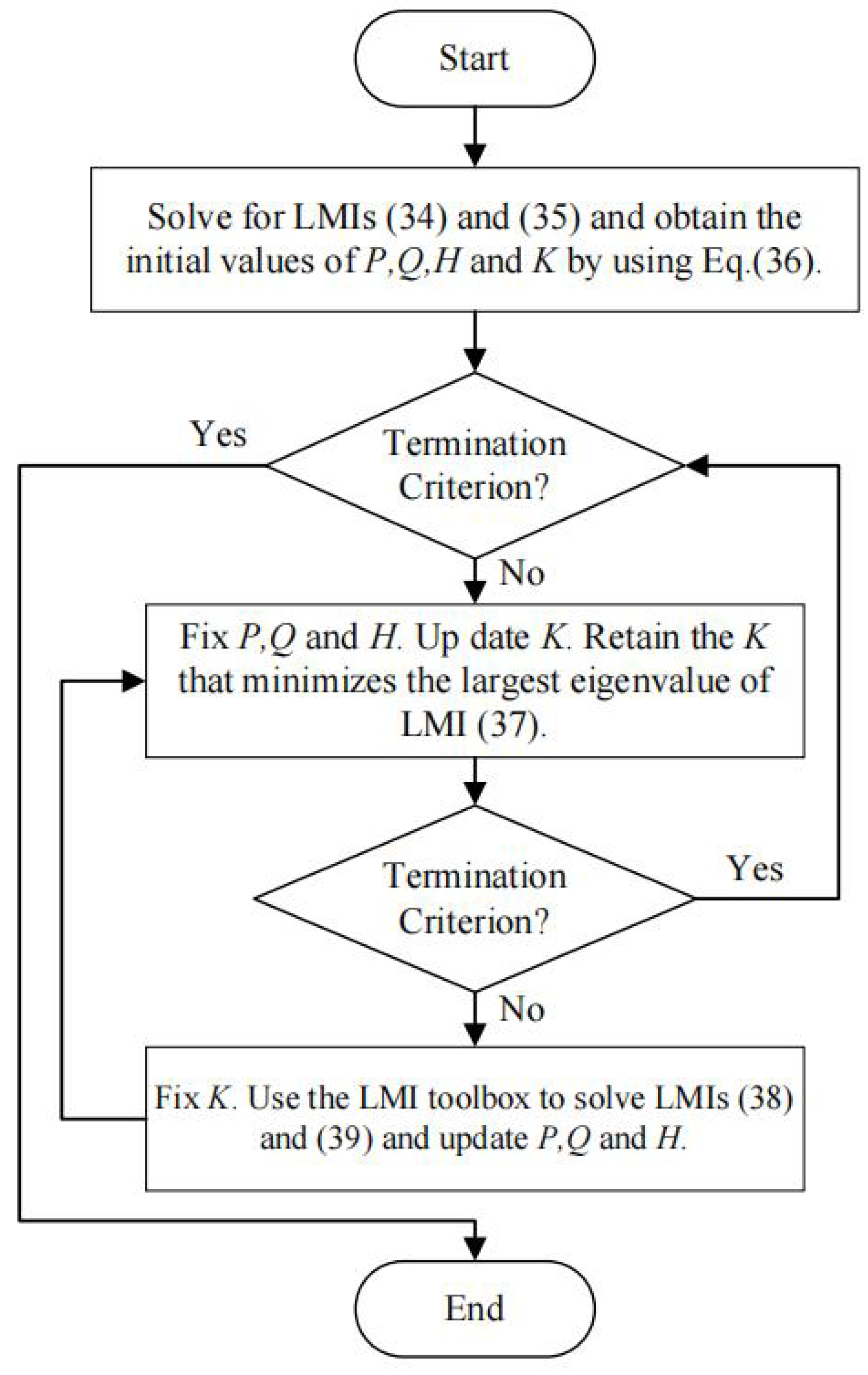
Figure 2.
Responses of the system states for as shown in Example 1
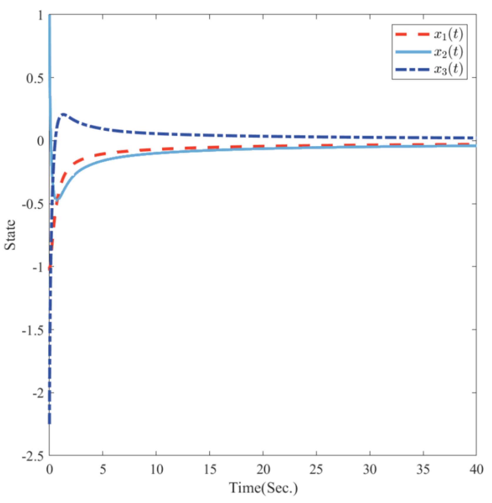
Figure 3.
Responses of the close-loop system states as shown in Example 2
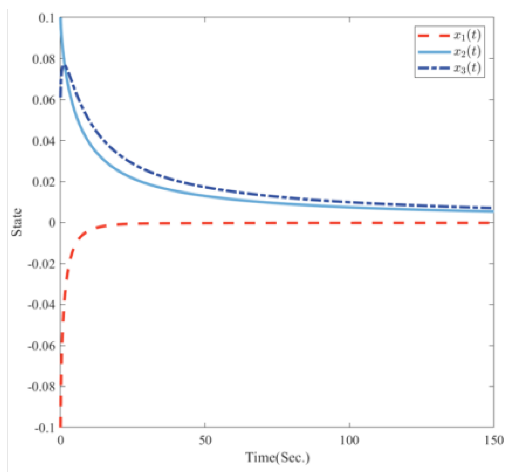
Figure 4.
Electrical circuit Illustration to Example 3
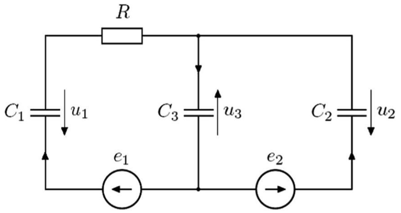
Figure 5.
Responses of the close-loop system states as shown in Example 3
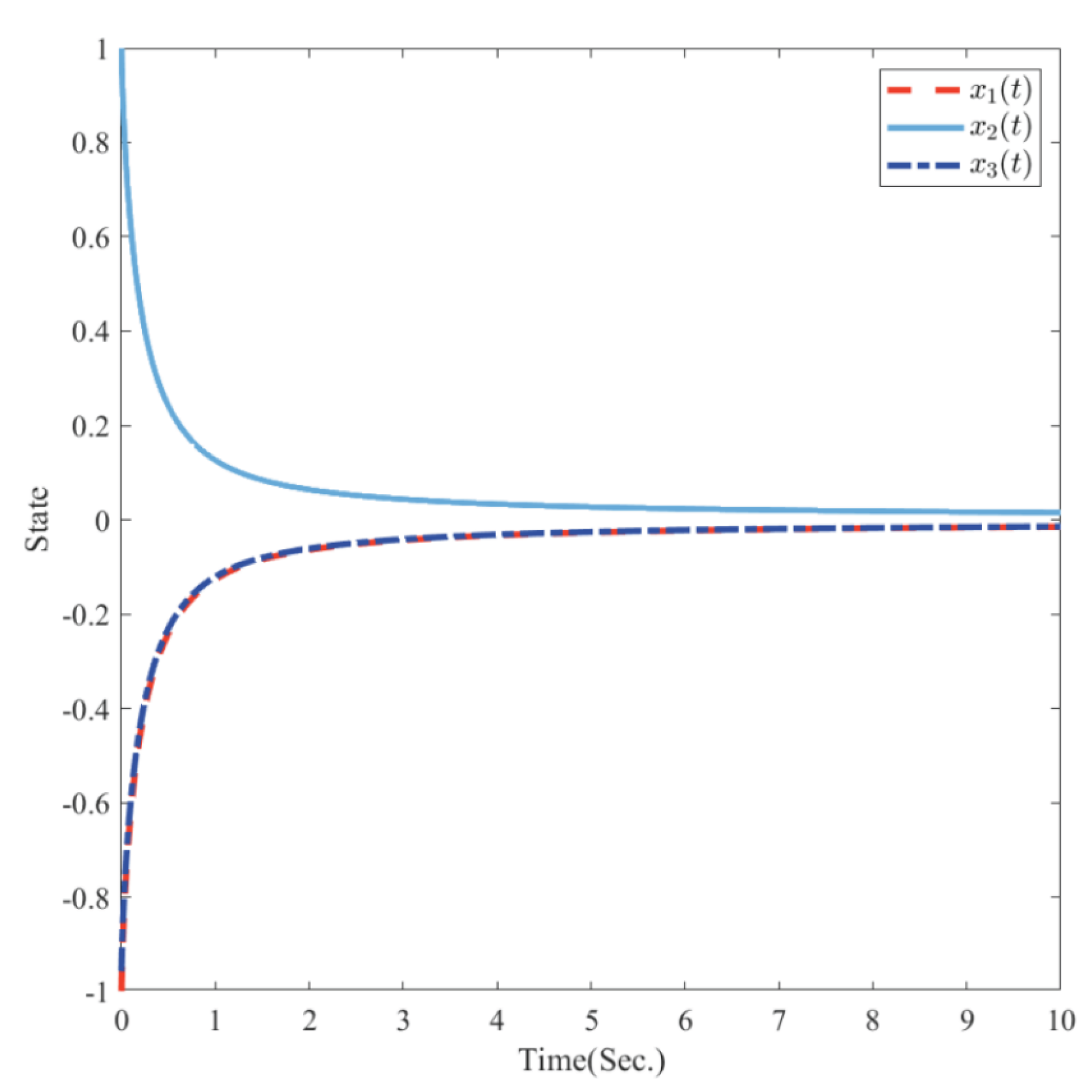

Table 1.
Comparison of the proposed approaches with existing approaches
| Ref. | System type | Fractional order field |
Variables | No equality constraints |
No bilinear problem |
|---|---|---|---|---|---|
| Theorem 3 in [24] | Singular FOSs | 6 | × | ||
| Theorem 2 in [25] | Singular FOSs | 5 | × | ||
| Theorem 1 in [22] | Singular FOSs | 4 | × | ||
| Theorem 1 in [21] | FOSs | 4 | |||
| Our Theorems 1 and 2 | Singular FOSs | 2/3 | |||
| Our Corollary 1 | Singular FOSs | 1 | |||
| Our Theorem 3 | Singular FOSs | 3 | × |
Disclaimer/Publisher’s Note: The statements, opinions and data contained in all publications are solely those of the individual author(s) and contributor(s) and not of MDPI and/or the editor(s). MDPI and/or the editor(s) disclaim responsibility for any injury to people or property resulting from any ideas, methods, instructions or products referred to in the content. |
© 2025 by the authors. Licensee MDPI, Basel, Switzerland. This article is an open access article distributed under the terms and conditions of the Creative Commons Attribution (CC BY) license (http://creativecommons.org/licenses/by/4.0/).
Copyright: This open access article is published under a Creative Commons CC BY 4.0 license, which permit the free download, distribution, and reuse, provided that the author and preprint are cited in any reuse.


