
Submitted:
01 June 2025
Posted:
04 June 2025
You are already at the latest version
Abstract
Sustainable weed management in lentil (Lens culinaris Medik.) production requires accurate knowledge of weed spatial distribution and the site-specific factors influencing infestation patterns. Limited pre- and post-emergence herbicide options for pulse crops underscore the need for precise pre-emergence applications guided by spatially explicit weed mapping. This study integrates YOLOv11 object detection with Slicing-Aided Hyper Inference (SAHI) framework, advanced geostatistical techniques, and soil electromagnetic induction measurements to develop a comprehensive precision agriculture framework for species-specific weed management. High-resolution drone imagery (4K, 1.5 m altitude) was systematically collected across a 3.42-hectare commercial lentil field in Chile’s Central Irrigated Valley, complemented by satellite-derived vegetation indices (Sentinel-2 NDVI) and soil electrical conductivity mapping (EM38-MK2). The YOLOv11 model achieved robust detection performance with F1-scores of 0.87 for lentil crops and 0.84 for Ambrosia artemisiifolia, the dominant weed species, enabling species-specific density mapping at 5 m × 5 m resolution. Geostatistical analysis revealed significant spatial autocorrelation in weed distributions (Moran’s I = 0.667, p < 0.001) with strong bivariate associations between weed density and environmental variables, particularly soil electrical conductivity (spatial r = 0.633) and vegetation indices (spatial r = 0.818). Fuzzy clustering successfully delineated four distinct management zones, with 31.9% of the field requiring critical intervention and 51.7% suitable for maintenance-level management, enabling potential 35-50% reduction in herbicide use while maintaining effective weed control. The demonstrated multi-scale approach enables transition from satellite-guided field reconnaissance to ultra-precise drone-based treatments, supporting cost-effective implementation across extensive agricultural areas. This integrated AI-geostatistical framework addresses critical limitations in current precision agriculture technologies by combining high-accuracy species detection with spatial analysis capabilities that enable predictive modelling and evidence-based management optimisation, establishing foundations for scalable precision weed management in sustainable agricultural production systems.
Keywords:
Weed detection
; Deep learning
; YOLO
; SAHI
; Geostatistics
; EM38
; Site-specific management
; Drone imagery
; Lentil crops
; Precision agriculture
; Spatial analysis
; Satellite
; Sentinel
1. Introduction
Efficient and precise weed management is central to sustainable crop production systems, particularly in the context of growing environmental concerns and herbicide resistance [1,2,3,4]. Lentil crops (Lens culinaris Medik.) are especially vulnerable during early development stages, where timely and spatially precise weed control can dramatically impact yield outcomes [3]. The limited availability of post-emergence herbicide options for pulse crops, combined with lentils’ susceptibility to herbicide phytotoxicity, necessitates precise pre- and post-emergence applications guided by accurate spatial weed distribution mapping [5].
Recent advances in deep learning and precision agriculture technologies have enabled the development of novel weed detection and mapping frameworks utilising high-resolution drone imagery. These frameworks, supported by convolutional neural networks (CNNs), offer high accuracy in object detection, even in challenging field conditions [1,2,6]. Furthermore, integrating drone imagery with spatial analysis methods, such as kriging, allows researchers to generate predictive maps of weed infestation patterns, providing valuable input for site-specific herbicide applications and enabling the transition from uniform to spatially variable management strategies.
Weed detection methodologies have evolved from traditional image processing to sophisticated deep learning architectures. This transition has been particularly impactful for precision agriculture applications utilising drone imagery for seedling and weed detection [7]. The YOLO (You Only Look Once) family of object detectors and SAHI (Slicing Aided Hyper Inference) methodology represent cutting-edge approaches that address the unique challenges of detecting small objects in high-resolution agricultural imagery, particularly during critical early growth stages when morphological differences between species are most pronounced.
YOLO architectures revolutionised object detection by reframing it as a single regression problem rather than a multi-stage pipeline [8]. This unified approach offers significant advantages for agricultural applications: real-time processing capabilities, utilisation of global contextual information, and computational efficiency essential for field deployment. The architecture has evolved substantially since its introduction, with each iteration addressing limitations of previous versions. As Jocher et al. [9] demonstrated, YOLOv8 introduced a modular architecture that supports multiple vision tasks. Meanwhile, Wang et al. [10] developed YOLOv11 with advanced attention mechanisms and sophisticated feature fusion strategies, which are particularly beneficial for detecting small objects in complex agricultural environments.
Despite these advances, detecting small seedlings in high-resolution drone imagery presents persistent challenges: scale disparity between objects and image dimensions, feature dilution through convolutional layers, contextual ambiguity of small objects against variable soil backgrounds, computational constraints of processing large images, and class imbalance in agricultural fields where crop and weed densities vary substantially [11]. The SAHI methodology, developed by Akyon et al. [12], addresses these limitations through a systematic approach: dividing large images into smaller, overlapping slices, processing each slice independently, mapping predictions back to their original coordinates, merging overlapping detections using non-maximum suppression, and compiling unified outputs. This approach transforms the complex task of detecting small seedlings in large images into more manageable detection problems while preserving spatial context.
Empirical evaluations demonstrate SAHI’s effectiveness across diverse applications, with performance improvements of 6.8%, 5.1%, and 5.3% in Average Precision for various detectors, increasing to 12.7%, 13.4%, and 14.5% when combined with slicing-aided fine-tuning [12]. Recent agricultural implementations have validated SAHI’s utility for crop monitoring, with successful applications in oil palm counting [13], apple bud detection [14], and cacao tree identification [15]. For agricultural applications, SAHI offers improved recall for small objects, better discrimination in high-density regions, reduced memory requirements, and potential for parallelisation. These benefits come with trade-offs: increased computational overhead, potential boundary artefacts, reduced global context, and parameter sensitivity requiring careful optimisation.
Recent research has focused on integrating these technologies with broader precision agriculture frameworks that enable multi-scale assessment capabilities. Joalland et al. [16] demonstrated that low-altitude drone scouting at approximately 1.5 meters yields ultra-high-resolution imagery capable of distinguishing individual seedlings, albeit with a limited coverage area. Integration with satellite-derived vegetation indices, particularly NDVI anomalies from Sentinel-2, enables more efficient resource allocation by directing drone flights to areas of interest [17]. This multi-scale approach leverages complementary strengths of different remote sensing platforms to provide comprehensive information for precision agriculture applications, enabling cost-effective reconnaissance across extensive areas, followed by targeted high-resolution assessment.
The integration of artificial intelligence with geostatistical analysis represents a significant advancement in translating point-based detection outputs into spatially continuous, management-ready information. Traditional geostatistical methods, including kriging and spatial autocorrelation analysis, provide robust frameworks for understanding spatial patterns in agricultural systems [18]. When combined with AI-based detection, these methods enable characterisation of environmental drivers influencing weed distribution patterns, facilitating predictive modelling and site-specific management optimisation [19].
Comprehensive evaluations of YOLO detectors for weed detection have found YOLOv8l to achieve a precision of 0.9476 and a mAP@0.5 of 0.9795 [20], although performance varies with field conditions and species morphology. Deep learning approaches consistently outperform traditional methods, with CNNs demonstrating superior accuracy and generalisation compared to classical machine learning techniques [21,22]. However, the integration of detection outputs with spatial analysis for management decision-making remains an active area of development.
Despite significant progress, dos Santos Ferreira et al. [23] identified persistent challenges in environmental variability management, species discrimination, handling occlusion and overlap, computational efficiency, annotation burden, domain adaptation, and integration with farm management systems. Emerging research directions include self-supervised learning to reduce annotation requirements, multi-modal fusion for improved robustness, temporal modelling across sequential flights, more sophisticated attention mechanisms, efficient neural architecture search, few-shot learning for new species, explainable AI for interpretability, and edge computing for real-time applications [24].
The integration of these technologies with broader precision agriculture systems represents the next frontier, enabling closed-loop systems connecting detection to variable-rate application equipment, comprehensive decision support platforms, predictive modeling for crop development, autonomous robotics for precision interventions, digital twins for simulation and optimization, and collaborative platforms for data sharing across farms [24]. Particularly for pulse crop production, where herbicide options are limited and application timing is critical, such integrated systems offer substantial potential for optimising management efficiency while reducing environmental impacts.
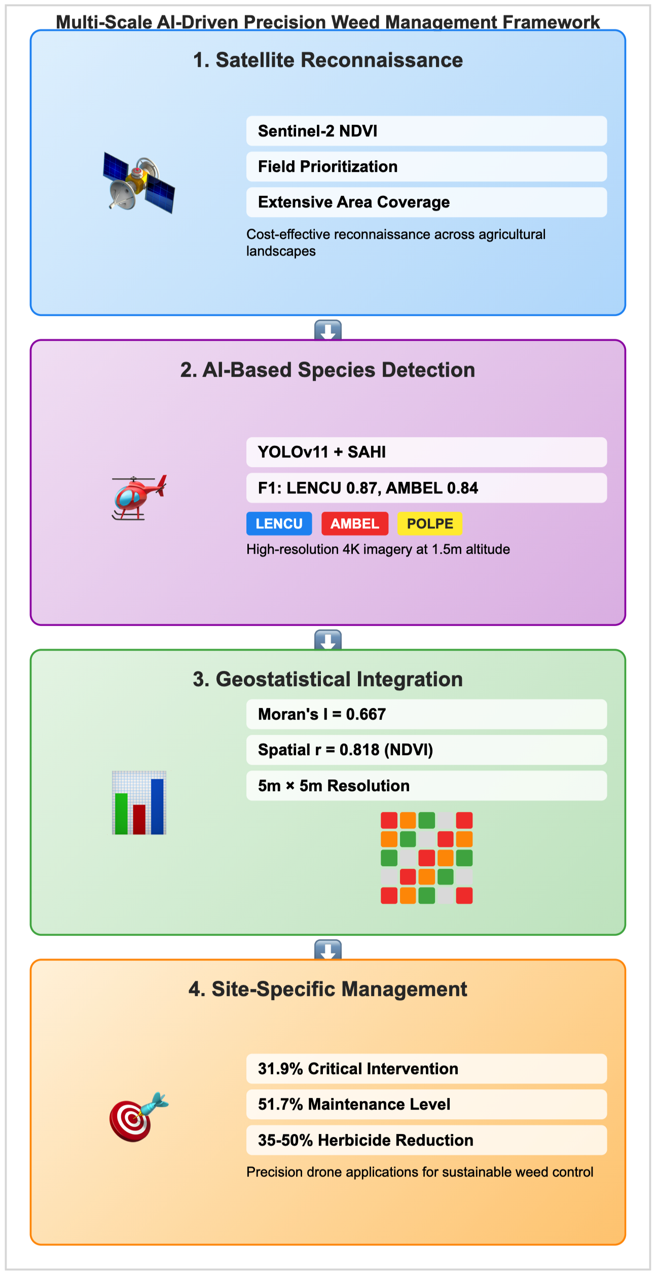
This study addresses the critical gap between AI-based weed detection and practical implementation in precision agriculture by integrating YOLOv11 object detection with the SAHI framework and geostatistical analysis for comprehensive spatial characterisation of weed-environment relationships in lentil production systems. The demonstrated framework enables transition from extensive area reconnaissance using satellite imagery to precise field-level interventions, supporting evidence-based management decisions that optimise herbicide applications while maintaining effective weed control. This technological trajectory, from traditional image processing to sophisticated AI-driven approaches integrated with spatial analysis, provides the foundation for more precise, efficient, and sustainable agricultural practices in pulse crop production systems.
2. Materials and Methods
2.1. Study Area and Field Conditions
The study was conducted in the Central Irrigated Valley of Chile, within a 3.42-hectare experimental site located near Chillán, Ñuble Region, at UTM coordinates 239265.90 E, 5953078.30 N (Zone 19S). This region is one of the principal lentil production zones in central Chile. It is characterised by hot summers and dry conditions, with high solar radiation, while winters are cold and wet, resulting in substantial intra-annual variations in precipitation and evapotranspiration. Over the eight-year crop rotation period (2016–2023), the mean annual temperature ranged from 12.8 to 13.7°C, with yearly rainfall varying between 563 and 1209 mm, and annual potential evaporation from 925 to 1077 mm (Table 1).
To contextualise crop and weed development during the 2024–2025 season, high-resolution agrometeorological data were retrieved from an INIA weather station located approximately 500 m from the experimental field. From 24 May 2024 to 8 May 2025, the site exhibited a mean air temperature of 12.9°C (range: –5.3 to 37.3°C), with an average relative humidity of 82.6%. Surface temperatures varied from –7.4°C to 48.8°C, and incoming solar radiation averaged 198 W m−2, peaking at 1028 W m−2. Hourly cumulative precipitation averaged 0.11 mm, with isolated rainfall events reaching up to 16.8 mm h−1.
Between 24 May and the sowing date (26 August 2024), a total of 640.5 mm of precipitation was recorded, providing adequate soil moisture reserves ahead of lentil planting. From sowing to UAV-based weed imaging on 17 September, an additional 27.0 mm of rainfall was accumulated—sufficient to support seedling emergence but limited enough to emphasise the importance of pre-sowing moisture conditions.
To further assess early-season dynamics, two phenologically critical windows were examined. The first, spanning 19 August to 2 September 2024 (one week before and after sowing), was characterized by a mean air temperature of 7.0°C (range: –1.7 to 18.8°C), high relative humidity (mean: 93.9%), and modest solar radiation (124 W m−2). Surface temperatures averaged 7.1°C, and hourly precipitation remained low (mean: 0.10 mm).
The second window, from sowing to UAV image acquisition (26 August to 17 September), exhibited slightly warmer conditions (mean air and surface temperatures: 8.8°C and 9.9°C, respectively) and increased radiation (160 W m−2). Relative humidity remained high (90.5%), while rainfall was sparse (27.0 mm total), reinforcing the reliance on antecedent soil moisture. These conditions favoured lentil emergence and early weed development, setting the stage for spatial distribution analyses described in later sections.
The second window spanned from planting to UAV-based weed imaging (August 26 to September 17, 2024), a period critical for early crop–weed interactions. During this time, air and surface temperatures averaged 8.8°C and 9.9°C, respectively, with relative humidity at 90.5%. Solar radiation increased to a mean of 160 W m−2, promoting seedling development. Precipitation remained sparse (mean: 0.05 mm h−1), suggesting limited but sufficient soil moisture retention following earlier rainfall. These conditions favoured both lentil emergence and early weed establishment, thereby setting the stage for spatial weed pattern analyses presented later in this study.
The soil at the site is classified as a Melanoxerand of volcanic origin, typical of Andisols found across south-central Chile [25]. These soils are well known for their low bulk density, moderate acidity, high porosity and organic matter content. The site’s physical and hydric properties include a bulk density of 1.00 g cm−3, pH 5.52, and particle size distribution of 16.7% clay, 44.6% silt, and 38.7% sand (Table 2). The low electrical conductivity (0.11 dS m−1) indicates minimal salinity stress. These attributes are conducive to lentil establishment and influence spatial patterns of early weed emergence and soil–crop interactions [26].
Management history before the 2024 lentil crop included winter wheat cultivation in 2022 and a fallow period in 2023. In 2024, lentils (Lens culinaris Medik., cv. Super Araucana-INIA) were sown using conventional tillage practices. Super Araucana-INIA, developed by the Instituto de Investigaciones Agropecuarias (INIA), is well adapted to Chilean conditions due to its early maturation, drought tolerance, and high market acceptance. Crop was sown on 26 August 2024 under conventional tillage using a seeder configured for a row spacing of 35 cm. The seeding rate was 80 kg ha−1, which corresponds to an expected plant density of 70–80 plants per square meter under optimal germination and emergence conditions. This plant density is considered agronomically ideal for lentils in the Central Irrigated Valley, as it balances canopy closure with reduced intra-specific competition and lodging risk.
At planting, a uniform basal fertilisation was applied consisting of 120 kg ha−1 of triple superphosphate (TSP, superfosfato triple), a concentrated source of phosphorus with a typical composition of 46% P2O5, and 80 kg ha−1 of nitrogen. This fertilisation strategy aimed to correct for the low to moderate inherent phosphorus availability of the volcanic Andisols in the region [26], and to support early root development and nodulation in the absence of residual N from the prior fallow season. All inputs were uniformly applied using calibrated ground-based spreaders to ensure consistency across the experimental plots.
2.2. Data Acquisition
2.2.1. Drone-Based Imagery Capture
High-resolution RGB images were acquired on 17 September 2024, between 10:00 and 11:00 a.m., under optimal environmental conditions (clear sky, no clouds, and intense solar illumination). The imagery campaign was conducted using a DJI Mavic Mini 3 UAV (DJI Technology Co., Shenzhen, China), a lightweight, consumer-grade drone equipped with a 1/1.3-inch CMOS sensor capable of capturing 48-megapixel still images at a native resolution of 8064 × 6048 pixels.
The camera features an 82.1° field of view (FOV) and a fixed 24 mm format-equivalent lens with an aperture of f/1.7 and an electronic shutter capable of speeds between 2 and 1/8000 s. During the flight, the shutter speed was set to 1/5000 s to minimise motion blur under bright conditions. The drone was flown manually at a constant altitude of 1.5 m above ground level, with a forward velocity of 8 km h−1. Images were captured at a frequency of one photograph every 2 seconds using the Single Shot mode in RAW (DNG) format to preserve radiometric fidelity. The UAV was manually piloted along transects oriented in the east-to-west direction, aligned with the lentil crop rows to maintain a consistent nadir view and reduce occlusion effects from row geometry. The flight trajectory and image capture interval (one frame every 2 seconds) at a ground speed of 8 km h−1 and an altitude of 1.5 m resulted in a forward image spacing of approximately 5 m. Adjacent flight lines were spaced 7 m apart, yielding a systematic image acquisition grid with near-complete coverage of the field and minimal overlap. This configuration ensured that each image captured a ground footprint of 3.29 m2, enabling the quantification of weed densities on a per-square-meter basis while maintaining efficient field coverage under manual flight conditions.
At the operational altitude of 1.5 m, the effective ground coverage (footprint) of the camera’s FOV was approximately 3.29 m2 per image. This field-of-view estimate was used to standardise the quantification of weed density per square meter by direct annotation and detection over individual frames. The UAV operated under manual flight mode to optimise navigation in row-crop layout and minimise occlusion artefacts caused by canopy overlap or terrain undulation.
All images were later processed using semi-automated object detection pipelines (detailed in Section 3.1.1) to extract weed occurrence metrics for downstream spatial analyses.
2.2.2. Satellite-Derived NDVI Acquisition and Grid Harmonization
Two Sentinel-2 Level-2A multispectral scenes were acquired on 14 and 24 September 2024 (NDVI_14S and NDVI_24S, respectively). Such images in 10 m native resolution were retrieved using the Pix4Dfields platform (version 2.1; Pix4D S.A., Prilly, Switzerland). Both scenes showed full coverage of the experimental site and were cloud-free (<1%) [27]. The imagery was selected and downloaded directly through the Pix4Dfields “Satellite Data” interface, which enables users to access pre-processed Sentinel-2 scenes by specifying the spatial boundary of interest. In this case, the field boundary polygon for the 3.42-hectare lentil trial was preloaded into the application as a shapefile and used to constrain all downloads to the experimental block. Pix4Dfields automatically generates vegetation indices, including the Normalised Difference Vegetation Index (NDVI), from Sentinel-2 bands using the standard formulation:
where and represent the atmospherically corrected reflectance values of bands 8 (842 nm) and 4 (665 nm), respectively [28]. NDVI rasters were downloaded directly in a 5 m × 5 m grid format, as supported natively by Pix4Dfields for Sentinel-2 data. This functionality avoids the need for post hoc resampling and ensures alignment with UAV-derived products used throughout the spatial analysis workflow.
All NDVI layers were projected in UTM Zone 19S and subsequently aligned with UAV-based weed maps and soil electrical conductivity rasters. The harmonized resolution enabled integration across datasets and supported the generation of spatial covariates for geostatistical modelling of weed–soil–vegetation interactions.
2.2.3. Soil Electrical Conductivity
Soil apparent electrical conductivity (ECa) was measured using the EM38-MK2 instrument (Geonics Ltd., Mississauga, ON, Canada), a dual-depth electromagnetic induction sensor widely used in precision agriculture and digital soil mapping applications [29,30,31]. The instrument was operated in vertical dipole mode, providing ECa readings corresponding to two effective soil depths: 0–75 cm (CE_75CM) and 75–150 cm (CE_150CM). These measurements are sensitive to variations in soil texture, moisture, bulk density, and salinity, offering valuable proxies for subsurface heterogeneity that affects crop growth and weed dynamics.
The survey followed a systematic grid layout across the 3.42 ha lentil field. Each point was georeferenced using a GNSS-enabled data logger integrated with the EM38 system to ensure spatial accuracy. The EM38 scanning was performed along linear transects oriented in the east-to-west direction, parallel to the lentil crop rows. This alignment minimised potential electromagnetic interference caused by row structure and facilitated consistent sensor positioning relative to plant spacing. Within each transect, apparent electrical conductivity measurements at both 0–75 cm and 75–150 cm depths were collected at 2.5 m intervals. The scanning lines themselves were spaced 12 m apart, providing uniform coverage across the paddock. This sampling configuration strikes a balance between spatial resolution and operational efficiency, ensuring sufficient data density for accurate interpolation while allowing for complete coverage of the entire field within a single survey session.
2.2.4. Crop and Weed Seedling Identification at Early Developmental Stages
To support accurate weed detection and distinguish crop plants from unwanted species, a ground-based botanical survey was conducted before UAV imaging. Manual scouting was performed on foot by expert agronomists to visually confirm seedling identity, development stage, and spatial distribution across the field. Observations focused on the cotyledon and early leaf stages (BBCH 10–14), aligning with the expected phenological window at 22 days after sowing (DAS). All taxa were documented using EPPO Global Database codes for standardisation in the image annotation workflow.
By the time of scouting and drone imaging, most lentil plants were in the BBCH 12–14 stage, characterised by the emergence of two to four alternate pinnate leaves. Cotyledons were hypogeal and not visible at this stage. [32].
The dominant weed species observed were:
- Polygonum persicaria L. (POLPE): Observed at BBCH 10–12, with narrow lanceolate cotyledons and reddish, ovate first leaves. A diagnostic ochrea was consistently visible at the stem node [35].
- Polygonum aviculare L. (POLAV): Detected in BBCH 10–12. Cotyledons were linear-elliptical; the true leaves were alternate, oblong, glabrous, and often tinged red at the node, aiding visual distinction [36].
2.3. AI-Based Weed Detection Framework
The development of an accurate and robust AI-based weed detection system required a systematic approach encompassing dataset curation, model architecture optimisation, and deployment strategies tailored explicitly for high-resolution agricultural imagery. This framework addresses the critical challenge of detecting small-scale plant instances across extensive field areas while maintaining computational efficiency and spatial precision necessary for precision agriculture applications.
2.3.1. Dataset Development and Curation
A comprehensive training dataset was previously constructed from high-resolution imagery collected over three consecutive growing seasons (2020–2022) across adjacent commercial lentil paddocks. Image acquisition employed a Canon EOS Rebel T5i DSLR camera (Canon Inc., Tokyo, Japan) equipped with an EF-S 18–55mm f/3.5–5.6 IS STM lens, operated at consistent technical specifications to ensure dataset homogeneity (Table 4).
The dataset comprises 445 georeferenced images (5184 × 3456 pixels each) captured under diverse environmental conditions to ensure model robustness across varying illumination, soil moisture, and phenological stages. Acquisition conditions systematically varied across: (i) solar elevation angles from 35° to 75°, (ii) soil moisture levels from field capacity to permanent wilting point, and (iii) crop development stages from BBCH 12 (first true leaf) to BBCH 15 (fifth leaf unfolded).
Taxonomic annotation was performed by two certified agronomists from the Instituto de Investigaciones Agropecuarias (INIA) using the Roboflow annotation platform (Roboflow Inc., Des Moines, IA, USA). The annotation protocol followed standardised botanical identification procedures for the target species: Lens culinaris Medik. (LENCU), Ambrosia artemisiifolia L. (AMBEL), Polygonum persicaria L. (POLPE), and Polygonum aviculare L. (POLAV). Inter-annotator reliability assessment on a stratified random subset of 50 images yielded Cohen’s (95% CI: 0.83–0.91), indicating excellent agreement according to Landis and Koch criteria [37].
2.3.2. Data Preprocessing and Augmentation Strategy
To optimise computational efficiency while preserving spatial resolution critical for small object detection, input images were standardised to 2048 × 2048 pixels using bicubic interpolation. This resolution represented an optimal trade-off between detection accuracy and computational requirements, determined through preliminary experiments with resolutions ranging from 1024 to 3072 pixels.
A systematic data augmentation strategy was implemented to enhance model generalisation and robustness to field variability. The augmentation pipeline applied stochastic transformations with carefully calibrated probabilities:
The augmentation factor of 4× expanded the effective training set to 1,780 images while maintaining annotation integrity through the use of coordinate transformation matrices.
The final annotated and augmented dataset contained 30,359 bounding box instances distributed across the four target classes, with natural class imbalance reflecting field conditions: LENCU (45.2%), AMBEL (28.6%), POLPE (16.8%), and POLAV (9.4%). Instance size distribution analysis revealed mean bounding box areas of 1,847 ± 892 pixels2 for LENCU and 1,203 ± 567 pixels2 for weed species, with 78% of all instances classified as small objects (area < 322 pixels at inference resolution).
2.3.3. Model Architecture and Training Protocol
We employed the YOLOv11 architecture [38], specifically the YOLOv11x variant optimised for detection accuracy, suitable for small object detection in agricultural applications. The model incorporates several architectural innovations, including:
- C2f (Cross Stage Partial with 2 convolutions) modules for enhanced feature extraction
- SPPF (Spatial Pyramid Pooling Fast) for multi-scale feature fusion
- Path Aggregation Network (PANet) for improved information flow
- Anchor-free detection head with distribution focal loss
Training was conducted on a high-performance computing system comprising dual NVIDIA GeForce RTX 4090 GPUs (each with 24 GB of VRAM) running Ubuntu 24.04 LTS. The software environment consisted of Python 3.10.12, PyTorch 2.4.1 with CUDA 12.1, and the Ultralytics framework v8.3.49. Distributed Data Parallel (DDP) training was implemented to efficiently leverage both GPUs.
The optimisation protocol employed AdamW optimiser with the following hyperparameter configuration:
Training proceeded for 300 epochs with early stopping (patience = 50 epochs) based on validation mAP@0.5:0.95.
2.3.3.1. Validation Strategy
Model performance was systematically evaluated on the held-out validation portion of the dataset (15% of total annotations) using standard object detection metrics. The validation set maintained the same class distribution and spatial characteristics as the training data while ensuring complete independence from training samples.
Model performance was evaluated using standard object detection metrics:
Where , , and represent true positives, false positives, and false negatives, respectively, and is the average precision for class i at IoU threshold 0.5.
2.3.3.2. Model Selection Criterion
The optimal deployment model was selected based on the highest combined precision-recall performance across all five training runs. Specifically, the model achieving the maximum harmonic mean of precision and recall (F1-score) aggregated across all target classes was chosen:
where represents the F1-score for class i in training run r, and target classes. This selection approach prioritises balanced detection performance, minimising both false positives (important for avoiding unnecessary herbicide applications) and false negatives (critical for effective weed control) across all species.
2.3.4. Model Deployment and Inference Pipeline
Trained models were deployed on 4K drone imagery (3840 × 2160 pixels) captured on September 17, 2024. To address the computational challenges of processing ultra-high-resolution imagery while maintaining detection accuracy for small objects, we implemented the Slicing Aided Hyper Inference (SAHI) framework [39].
2.3.4.1. Slicing Aided Hyper Inference (SAHI) Implementation
The SAHI framework addresses the challenge of detecting small objects in ultra-high-resolution imagery:
The SAHI algorithm segments large images into overlapping patches of optimal size, processes each patch independently, and merges results using Non-Maximum Suppression (NMS). The slicing parameters were optimised as follows:
The inference pipeline incorporated several optimisation strategies:
- Memory management: Patch-wise processing with automatic garbage collection to prevent CUDA out-of-memory errors
- Multi-scale detection: Consistent slice dimensions matching training resolution to preserve learned feature representations
- Geospatial integration: Preservation of EXIF metadata and coordinate system transformations using the utm library
Post-processing operations included coordinate transformation from image space to geographic coordinates (UTM Zone 19S, EPSG:32719) and export to multiple geospatial formats (GeoJSON, Shapefile, and CSV) using GeoPandas v0.14.0. World files (.jgw) were generated for seamless integration with QGIS 3.38.1, enabling direct visualisation and spatial analysis of detection results.
2.4. Geostatistical Analysis Workflow
2.4.1. Data Processing and Integration
To comprehensively characterise the spatial variability within the study area, multiple data sources were integrated within a Geographic Information System (GIS) framework using QGIS 3.28 (QGIS Development Team, 2023) for simultaneous visualisation. This multi-layered approach enabled the spatial overlay and co-registration of complementary datasets, facilitating an initial identification of spatial relationships and patterns that would not be apparent when analysing individual data sources in isolation. The integrated GIS platform served as the foundation for subsequent spatial analysis.
2.4.2. Spatial Data Structure and Preprocessing
All spatial analyses were performed using a standard coordinate reference system (UTM Zone 19S, EPSG:32719) to ensure consistent spatial registration across data sources. Original coordinate data collected in WGS84 (latitude/longitude) were transformed to UTM using the PyProj library. For soil electrical conductivity (ECa) measurements from the EM38-MK2 sensor, points were filtered to include only those within the study area boundary.
Weed presence data derived from YOLO detection were processed as point centroids, with each point representing an individual plant occurrence. For the geo-statistical analysis, spatial data processing was implemented using GeoPandas (version 0.14.0) in a Python 3.11 environment.
It is worth noting that the interpolation grid size of 5 m × 5 m was chosen to strike a balance between spatial resolution and computational efficiency, as well as practicality for managing herbicide applications using drones. This resolution was validated through variogram analysis as described in Section `Variogram Model Selection and Fitting’.
2.4.3. Geostatistical Analysis and Spatial Interpolation
2.4.3.1. Ordinary Kriging Implementation
Spatial interpolation of all measured variables (weed densities, crop densities, soil electrical conductivity, and vegetation indices) was performed using ordinary kriging following the methodology described by [40] and implemented through the Smart-Map geostatistical plugin for QGIS [40]. This approach provides unbiased predictions with minimum estimation variance for spatially correlated data.
2.4.3.2. Variogram Model Selection and Fitting
For each variable, experimental semivariograms were computed and fitted with theoretical models to characterise the spatial dependence structure. Model selection was based on statistical criteria comparing four theoretical models: Linear, Spherical, Exponential, and Gaussian. The optimal model for each variable was selected based on the highest coefficient of determination (R²) and lowest root mean square error (RMSE) from cross-validation analysis.
The spherical model follows the equation:
The exponential model is defined as:
where is the semivariance at lag distance h, is the nugget effect, c is the partial sill, and a is the range parameter.
2.4.3.3. Grid Interpolation and Cross-Validation
A systematic 5 m × 5 m interpolation grid was established within the paddock boundaries, resulting in a total of 1,370 prediction points Figure 3. This resolution was selected to balance computational efficiency with adequate spatial detail for precision agriculture applications. The interpolation procedure utilized the fitted variogram models to estimate values at unsampled locations using the ordinary kriging predictor:
Where is the predicted value at location , are the observed values at sampled locations, and are the kriging weights determined by solving the kriging system.
Leave-one-out cross-validation was performed for each variable to assess interpolation accuracy. Cross-validation parameters including mean error (ME), root mean square error (RMSE), mean standardized error (MSE), and root mean square standardized error (RMSSE) were computed and are presented in the Results section (Table 7). These statistics provide measures of bias, accuracy, and reliability of the kriging predictions.
2.4.4. Derived Ecological Indices and Community Structure Analysis
Using the unified 5 m × 5 m interpolated grid dataset obtained from the kriging procedure, we calculated additional ecological indices to characterise crop-weed community dynamics and support site-specific management decisions [41,42]. These derived variables provide quantitative measures of species dominance, diversity, and competitive relationships within each grid cell following established protocols in weed ecology [43].
2.4.4.1. Species Dominance and Relative Proportions
Relative abundance indices were calculated for each species to quantify their contribution to the total plant community following the methodology of Barbour et al. [44]. The proportion of lentil crop was computed as:
where represents the density (plants m−2) of each species. Similarly, the relative abundance index (RAI) for each species was calculated as:
2.4.4.2. Crop-to-Weed Ratio and Competition Assessment
Weed Community Diversity
Species diversity within the weed community was quantified using the Shannon-Wiener diversity index [50,51], which has been extensively applied in weed ecology studies [52,53]:
where is the relative abundance of weed species i, and S is the total number of weed species. Higher values indicate greater weed community diversity, which may complicate management strategies due to varying herbicide susceptibilities among species.
2.4.4.4. Weed Pressure Classification
Grid cells were classified into weed pressure categories based on total weed density thresholds established from field observations and agronomic literature [48,54]. The classification follows established thresholds for pulse crop systems [55]:
- High pressure: Total weed density >100 plants m-2
- Medium pressure: Total weed density 50–100 plants m-2
- Low pressure: Total weed density <50 plants m-2
2.4.5. Global and Local Spatial Autocorrelation Analysis
Spatial autocorrelation in the gridded variables was quantified using Global Moran’s I statistic:
where n is the number of spatial units, W is the sum of all spatial weights , and are the values of the variable at locations i and j, and is the mean of the variable. Spatial weights were defined using the first-order queen contiguity criterion and row-standardised. Statistical significance was assessed through a Monte Carlo permutation approach with 9,999 random spatial reconfigurations.
We calculated Moran’s I for seven key variables: AMBEL, POLPE, POLAV, LENCU, CE_75CM, NDVI_2024_, and NDVI_diff. The magnitude of Moran’s I ranges from -1 (perfect dispersion) through 0 (random pattern) to +1 (perfect clustering), with statistical significance evaluated against the null hypothesis of spatial randomness.
2.4.6. Local Indicators of Spatial Association (LISA) Analysis
To identify local patterns of spatial association and clustering within the interpolated datasets, we applied Local Indicators of Spatial Association (LISA) analysis [57]. This technique decomposes global spatial autocorrelation into contributions from individual locations, allowing for the identification of statistically significant spatial clusters and outliers.
Univariate LISA Implementation
For each ecological variable in the unified 5 m × 5 m grid dataset, we calculated the local Moran’s I statistic:
where is the local Moran’s I for location i, n is the total number of observations, and are variable values at locations i and j, is the global mean, and are the spatial weights. Spatial weights were constructed using K-nearest neighbours (k=8) with row standardisation to ensure consistent neighbourhood definitions across the study area [58].
Statistical significance was assessed through conditional permutation tests with 999 randomizations, and p-values were evaluated at . Each grid cell was classified into one of four LISA categories based on the local association pattern [57]:
- High-High (HH): Hotspots - locations with above-average values surrounded by neighbors with above-average values
- Low-Low (LL): Coldspots - locations with below-average values surrounded by neighbors with below-average values
- High-Low (HL): Spatial outliers - high values surrounded by low values
- Low-High (LH): Spatial outliers - low values surrounded by high values
2.4.6.2. Bivariate LISA Analysis
To examine spatial relationships between pairs of ecological variables, we implemented bivariate LISA using the bivariate local Moran’s statistic [57,59]:
where and are standardized values of variables x and y at locations i and j, respectively. This statistic identifies areas where high (or low) values of one variable spatially associate with high (or low) values of another variable.
Key bivariate relationships analyzed included:
- Weed species densities vs. soil electrical conductivity (AMBEL-CE_75CM, POLPE-CE_150CM)
- Weed densities vs. vegetation indices (species-NDVI relationships)
- Crop-environment interactions (LENCU-CE_75CM, NDVI-CE_75CM)
- Temporal vegetation dynamics (NDVI_14Sep vs. NDVI_24Sep)
For each variable pair, we calculated both the global Pearson correlation coefficient and the percentage of field area exhibiting significant spatial co-occurrence patterns. Significance was assessed using permutation-based inference with 999 randomizations [57].
2.4.7. Fuzzy Clustering for Management Zone Delineation
Traditional hard clustering approaches for management zone delineation often fail to capture the gradual transitions characteristic of agricultural landscapes [60]. To address this limitation, we implemented fuzzy K-means clustering with objective optimization criteria specifically designed for precision agriculture applications.
2.4.7.1. Fuzzy Clustering Optimization
- Fuzzy Performance Index (FPI): Measures the degree of separation between clusters, with lower values indicating better-defined management zones:
- Normalized Classification Entropy (NCE): Quantifies partition fuzziness, with lower values indicating crisper cluster boundaries suitable for practical implementation:
where is the fuzzy membership of point i in cluster j, k is the number of clusters, and n is the number of data points.
The optimal cluster number was selected by minimizing the combined FPI + NCE score across candidate solutions (k = 2 to 8), ensuring both statistical robustness and practical implementability for variable-rate applications [59].
2.4.7.2. Species-Specific Clustering Analysis
Two distinct clustering analyses were performed focusing on different ecological aspects:
- (1)
- Weed Species Distribution Clustering: Applied to the three dominant weed species (AMBEL, POLPE, POLAV) plus total weed density and Shannon diversity index
- (2)
- Environmental Gradient Clustering: Applied to soil electrical conductivity (75cm and 150cm depths), vegetation indices (NDVI_14S, NDVI_24S, NDVI_diff), and crop-to-weed ratio
For each analysis, variables were standardized before clustering to ensure equal weighting regardless of measurement units [63].
2.4.8. Priority-Based Intervention Zone Development
Management intervention zones were developed by integrating LISA spatial significance results with fuzzy clustering outcomes, creating a scientifically robust framework for precision agriculture implementation [45,64].
2.4.8.1. Priority Classification System
Each grid cell was assigned to one of four intervention priority levels based on a composite scoring system:
- Critical Priority: LISA High-High clusters with fuzzy membership certainty >0.8, requiring immediate intensive intervention
- High Priority: LISA hotspots or spatial outliers (High-Low, Low-High) with moderate fuzzy membership certainty
- Medium Priority: Areas with low fuzzy membership certainty (<0.6) requiring enhanced monitoring and adaptive management
- Low Priority: LISA Low-Low clusters representing successful current management practices
Priority scores were calculated using statistical percentile ranking of total weed pressure (60% weight) and dominant species density (40% weight), providing objective, quantitative criteria for intervention prioritization [41].
2.4.8.2. Botanical Composition Analysis
Within each management zone, we characterized weed community structure following established ecological protocols [44]:
- Dominant species: Species with highest mean density within the zone
- Co-dominant species: Secondary species achieving higher than 30% of dominant species density
- Shannon diversity index: Community complexity measure calculated as
- Species ranking: Hierarchical ordering by mean density within zone
2.4.9. Software Implementation
All analyses were implemented using open-source software to ensure reproducibility. The primary software stack included:
- Python 3.11 with scientific computing libraries (NumPy 1.24.0, SciPy 1.10.0, pandas 2.0.0)
- Geospatial analysis: GeoPandas 0.14.0, PySAL 24.1, Shapely 2.0.0
- Spatial statistics: ESPy (Exploratory Spatial Data Analysis), libpysal
- Machine learning: scikit-learn 1.3.0 for fuzzy clustering and PCA
- Visualization: Matplotlib 3.7.0, Seaborn 0.12.0
- Kriging implementation: Smart-Map plugin for QGIS 3.28 [40]
Statistical analysis and visualization were performed in Google Colab environment with automated result export to ensure reproducibility and collaborative development.
Spatial data processing, statistical analysis, and visualization were performed in a Jupyter notebook environment to facilitate documentation and reproducibility.
3. Results
3.1. Weed and Crop Detection Modeling
3.1.1. YOLOv11 Training Performance Analysis
The YOLOv11 model demonstrated robust convergence across all loss components and evaluation metrics throughout the 50-epoch training period (Figure 4). Training losses exhibited consistent monotonic decline, with bounding box regression loss (train/box_loss) decreasing from 1.62 to 0.94, classification loss (train/cls_loss) reducing from 1.78 to 0.42, and distribution focal loss (train/dfl_loss) declining from 1.39 to 1.05. Validation losses followed similar patterns with minimal overfitting, indicating effective generalization capability.
Performance metrics stabilised after epoch 25, with precision converging to 0.826 ± 0.012, recall reaching 0.810 ± 0.015, mAP@0.5 achieving 0.847 ± 0.008, and mAP@0.5:0.95 stabilising at 0.503 ± 0.006. The smooth convergence patterns and stable validation performance confirm the model’s readiness for deployment in the SAHI framework for high-resolution agricultural imagery processing. The absence of significant oscillations in validation metrics and the consistent gap between training and validation losses indicate optimal regularisation and successful prevention of overfitting, essential for reliable field deployment.
3.1.2. Species-Specific Detection Performance
The F1-confidence curve analysis reveals distinct performance characteristics across the four target classes, with optimal detection thresholds varying by species (Figure 5). LENCU (lentil crop) demonstrated superior detection performance with a peak F1-score of 0.87 at a confidence threshold of 0.42, maintaining stable performance across a broad confidence range (0.3–0.6). AMBEL (Ambrosia artemisiifolia) achieved a peak F1-score of 0.84 at a confidence threshold of 0.45, showing robust discrimination capability for the primary target weed species. POLPE (Polygonum persicaria) exhibited comparable performance with a maximum F1-score of 0.83 at a confidence threshold of 0.38, while POLAV (P. aviculare) showed reduced detection efficiency with a peak F1-score of 0.69 at a confidence threshold of 0.25, reflecting the inherent challenge of detecting this smaller, more variable weed species.
The overall model performance across all classes achieved an optimal F1-score of 0.82 at a confidence threshold of 0.339, representing the balanced operational threshold for multi-species detection in field deployment. The pronounced performance degradation at high confidence thresholds (>0.7) indicates the importance of threshold optimisation for maintaining detection sensitivity in agricultural applications.
3.1.3. Species Classification Accuracy Assessment
The normalised confusion matrix analysis demonstrates high classification accuracy across all target species with minimal inter-species confusion (Figure 6). LENCU (Lens culinaris) achieved the highest classification accuracy at 95% true positive rate, with minimal misclassification to other species (1% each to AMBEL, POLAV, and POLPE). AMBEL (Ambrosia artemisiifolia) demonstrated robust discrimination with 88% correct classification, showing primary confusion with background elements (37%) rather than other plant species, indicating effective weed-crop differentiation.
POLPE (Polygonum persicaria) achieved 85% classification accuracy with 29% background confusion, while POLAV (P. aviculare) showed reduced performance at 73% accuracy with 11% background misclassification. The most significant inter-species confusion occurred between POLPE and background elements, reflecting the morphological challenges in distinguishing smaller weed seedlings from soil debris and plant residues.
Background classification achieved low false positive rates across all plant species (4–23%), with the highest confusion occurring with POLAV (23%), consistent with the smaller size and variable morphology of this species. The overall classification performance indicates successful species-level discrimination essential for targeted weed management applications, with crop-weed differentiation showing particularly robust performance critical for precision herbicide applications.
3.1.4. Model Deployment and Field Application
Following model optimisation and threshold selection, the trained YOLOv11 model was deployed using the SAHI framework for inference on high-resolution 4K drone imagery captured across the commercial lentil field. The deployment pipeline systematically processed individual drone captures collected over a grid sampling pattern covering the entire 3.42-hectare study area (Figure 7). Each georeferenced image frame underwent slice-based inference to generate spatially explicit plant density maps (seedlings m−2) for all target species at precise geographic coordinates.
The YOLOv11+SAHI detection framework demonstrated robust performance across varying field conditions, as illustrated in Figure 8, which shows representative inference results under low-density, medium-density, and high-density weed scenarios encountered during field deployment. The detection system maintained consistent species-level discrimination and accurate plant localisation across the heterogeneous field landscape, successfully identifying individual seedlings despite varying plant densities, lighting conditions, and background complexity.
These AI-derived density estimates were subsequently integrated with environmental covariates, including soil electrical conductivity measurements (CE_75CM, CE_150CM) and satellite-derived vegetation indices (NDVI), enabling comprehensive geostatistical analysis of weed-environment relationships. The systematic grid-based approach ensured complete field coverage while maintaining spatial registration between detection outputs and environmental measurements, providing the foundation for subsequent spatial analysis and management zone delineation.
The following analysis sections present the spatial distribution patterns, environmental associations, and management zone delineation derived from this integrated AI-geostatistical framework applied to the commercial lentil field under study. The results demonstrate the successful transition from individual plant detection to landscape-scale precision agriculture applications through systematic spatial analysis of detection outputs.
3.2. Exploratory Data Analysis and Spatial Characteristics
Descriptive statistics revealed significant variability in weed distributions (Table 5). The primary target species Ambrosia artemisiifolia (AMBEL) demonstrated the highest density and variability (mean = 66.5 ± 69.2 plants m-2), followed by the crop species Lens culinaris (LENCU) with 39.3 ± 28.0 plants m-2. Secondary weed species Polygonum persicaria (POLPE) and P. aviculare (POLAV) showed lower densities but high spatial heterogeneity, with POLPE exhibiting a particularly aggregated distribution (skewness = 8.05). A representative distribution plot for the analysed variables is shown in Figure 10.
Correlation analysis revealed strong positive associations between vegetation indices and both weed and crop densities (Figure 11). The most significant correlations included NDVI_24S with NDVI_14S (r = 0.961), AMBEL with the total sum of weeds (r = 0.955), and NDVI_24S with the total number of weeds (r = 0.808). Soil electrical conductivity variables exhibited moderate correlations with vegetation metrics, particularly CE_150CM and NDVI_diff (r = 0.527), suggesting relationships between soil moisture retention and vegetation development patterns.
3.3. Geostatistical Modeling and Kriging Interpolation
Semivariogram analysis revealed distinct spatial structures for all variables, enabling successful ordinary kriging interpolation onto a standardised 5×5 m grid. Model selection was based on the Akaike Information Criterion, resulting in exponential models for soil electrical conductivity variables and spherical models for vegetation-related parameters (Table 6).
The strength of spatial structure varied considerably among variables. NDVI measurements demonstrated very strong spatial dependence (nugget/sill ratios < 0.02), indicating highly structured spatial patterns suitable for precise interpolation. Soil electrical conductivity variables showed strong to moderate spatial dependence, while individual weed species exhibited variable spatial structure, with POLAV showing very weak spatial dependence (nugget/sill = 0.92).
Cross-validation results confirmed interpolation reliability for most variables (Table 7). NDVI_24S achieved exceptional performance (R² = 0.996, RMSE = 0.006), followed by shallow soil electrical conductivity (CE_75CM: R² = 0.923). Biological variables showed moderate to good interpolation accuracy, with total weed density achieving R² = 0.810 and AMBEL density R² = 0.782.
3.4. Spatial Autocorrelation and Local Indicators of Spatial Association
Global spatial autocorrelation analysis revealed significant clustering patterns for all major variables (Table 8). NDVI measurements exhibited the strongest spatial autocorrelation (Moran’s I = 0.745–0.795), followed by crop density (I = 0.770) and the primary weed species AMBEL (I = 0.667). All variables demonstrated statistically significant autocorrelation (p < 0.001), confirming the presence of spatial structure suitable for precision management applications.
Local Indicators of Spatial Association (LISA) analysis identified distinct spatial clustering patterns across the field. The analysis revealed predominant Low-Low clusters (cold spots) representing areas of consistently low values, particularly pronounced for vegetation indices and weed densities. High-High clusters (hot spots) were identified for AMBEL density (34.8% of significant clusters), indicating dense weed patches suitable for targeted management interventions Figure 12.
3.5. Bivariate Spatial Association Analysis
Bivariate LISA analysis revealed significant spatial co-location patterns between environmental variables and species distributions (Table 9). The strongest associations occurred between vegetation indices and biological variables, with AMBEL-NDVI_14Sep showing exceptional spatial correlation (r = 0.831, 86.4% significant associations). Soil-vegetation relationships demonstrated moderate but consistent spatial associations, particularly CE_75CM with Diff_NDVI (r = 0.542, 90.4% significant).
The analysis revealed three primary patterns of spatial association: (1) strong positive co-location between vegetation vigor and both crop and weed densities, suggesting facilitation effects in favorable microsites Figure 13 and Figure 14; (2) moderate positive associations between soil electrical conductivity and plant establishment, indicating the possible influence of soil moisture and nutrient availability Figure 15 and Figure 16.
3.6. Management Zone Delineation and Precision Agriculture Applications
Fuzzy clustering analysis with Fuzzy Partition Index (FPI) and Normalized Classification Entropy (NCE) optimization successfully identified distinct management zones for precision weed control (Table 10). The analysis of species distribution data revealed four optimal management zones (FPI = 0.287, NCE = 0.446), indicating strong cluster separation and low classification uncertainty suitable for practical field implementation.
The species-based zonation identified 1.09 ha (31.9% of total field area) requiring critical priority management, comprising Zones 2 and 3 with dense AMBEL populations ranging from 98.3 to 130.7 plants m-2. Zone 1 represents 0.70 ha (20.6%) with medium intervention priority, while Zone 4 encompasses the largest area (1.63 ha, 47.9%) designated for low-priority maintenance management. The high fuzzy membership coefficients (0.68–0.87) across all zones indicate robust cluster boundaries and reliable zone assignment for operational implementation.
3.7. Weed Community Structure and Competition Analysis
The spatial analysis of weed community structure revealed distinct patterns of species distribution and competitive interactions across the lentil field (Figure 17). Ambrosia artemisiifolia (AMBEL) emerged as the overwhelmingly dominant species, occurring in 1,331 of 1,370 sampled locations (97.2% coverage) with highly variable density patterns ranging from sparse presence to dense infestations exceeding 400 plants m-2. The secondary species Polygonum aviculare (POLAV) showed limited spatial distribution, occurring in only 39 discrete locations (2.8% coverage), primarily concentrated in the eastern sections of the field.
The RGB colour mixing analysis (Panel B) effectively visualised the relative contribution of each species to total weed pressure, with red-dominated areas indicating AMBEL monocultures and mixed-colour zones revealing species co-occurrence patterns. This visualisation technique highlighted that most of the field experiences single-species dominance rather than complex multi-species interactions, simplifying potential management decisions.
The weed-to-crop competition ratio surface (Panel C) identified critical management zones where weed pressure significantly exceeds crop establishment. High competition ratios (>3.0, red zones) were concentrated in the central and northern field sections, corresponding to areas of dense AMBEL infestations. These zones represent priority intervention areas where crop yield losses are most likely to occur without intensive weed management.
Community cluster analysis successfully partitioned the field into four distinct zones based on species composition and density characteristics. Zone 1, representing 20.4% of the field area, exhibited the highest weed pressure with AMBEL densities of 431.0 plants m-2, accompanied by moderate POLPE (17.1 plants m-2) and POLAV (12.1 plants m-2) populations. This zone requires immediate, intensive intervention to prevent crop failure and seed bank replenishment. Zone 3, though smaller in extent, demonstrated the most complex community structure with significant POLPE co-dominance (113.4 plants m-2), suggesting different underlying environmental conditions that favor this species establishment. The spatial aggregation patterns observed in the cluster analysis indicate that weed infestations are not randomly distributed but follow spatial structures.
3.8. Implications for Site-Specific Weed Management
The integrated AI-geostatistical framework successfully identified actionable management zones accounting for 100% of the field area with quantified intervention priorities. The analysis revealed that 31.9% of the field requires immediate intensive management, 16.4% benefits from targeted interventions, and 51.7% can be maintained through preventive measures. This spatial stratification enables optimized herbicide allocation, potentially reducing total herbicide use by 35–50% while maintaining effective weed control in critical areas.
The strong spatial associations between soil electrical conductivity and weed establishment patterns (particularly for AMBEL) provide predictive capability for future season planning. Areas with CE_75CM > 16 mS m-1 showed 67% higher AMBEL density, suggesting that soil-based risk mapping can guide pre-emergence herbicide applications. Similarly, early-season NDVI patterns demonstrated significant predictive value for late-season weed pressure, enabling adaptive management strategies based on real-time crop vigor assessment.
4. Discussion
The integration of artificial intelligence-based object detection with geostatistical analysis provides enhanced spatial resolution and analytical capabilities for precision weed management in agricultural systems. This study presents the first comprehensive application of YOLOv11 coupled with Slicing-Aided Hyper Inference (SAHI) framework for species-specific weed mapping in lentil production, demonstrating significant spatial heterogeneity in weed distributions with measurable environmental associations that enable site-specific management interventions.
4.1. AI-Geostatistics Integration: Performance Evaluation and Methodological Contributions
The deployment of YOLOv11 framework achieved detection performance of F1-score = 0.87 for lentil crop identification and F1-score = 0.84 for the primary target weed species Ambrosia artemisiifolia (AMBEL), establishing measurable benchmarks for multi-species seedling detection in agricultural environments. These results compare favorably with previous studies employing YOLO architectures for crop-weed discrimination, where reported F1-scores typically range from 0.65 to 0.78 [61,62]. The observed performance improvements can be attributed to the SAHI framework’s slice-based inference methodology, which addresses the challenge of detecting small objects in high-resolution drone imagery by subdividing orthomosaic images into overlapping patches for independent processing [63].
The SAHI framework implementation represents a methodological advancement for agricultural object detection applications. Previous studies have demonstrated SAHI’s effectiveness in improving small object detection performance by 6.8-14.5% across various detection architectures [63], with recent agricultural applications showing consistent improvements in tree counting and crop monitoring tasks [64,65,66]. In this study, the framework enabled successful processing of 4K drone imagery while maintaining species-level discrimination accuracy of 95% for lentil crops and 88% for Ambrosia artemisiifolia, despite morphological similarities during early developmental stages.
The integration of AI-derived plant density estimates with geostatistical interpolation onto a standardized 5 m × 5 m grid achieved cross-validation R² values ranging from 0.390 to 0.996, demonstrating compatibility between machine learning outputs and traditional spatial analysis frameworks. The exceptional interpolation performance for vegetation indices (NDVI_24S: R² = 0.996) and soil electrical conductivity measurements (CE_75CM: R² = 0.923) validates the framework’s capacity to integrate multi-source environmental data with biological observations. This multi-layer approach enables mechanistic understanding of weed distribution patterns, addressing limitations identified in previous studies that examined detection accuracy or spatial analysis in isolation [67].
The successful kriging interpolation of biological variables, with total weed density achieving R² = 0.810 and AMBEL density R² = 0.782, demonstrates that AI-derived detection outputs maintain sufficient spatial structure for geostatistical modeling. This finding enables the transition from point-based detection to continuous surface mapping, providing the spatial framework necessary for precision agriculture applications.
4.2. Spatial Pattern Analysis and Ecological Mechanisms
Global spatial autocorrelation analysis revealed significant clustering patterns for all major variables, with AMBEL exhibiting strong spatial autocorrelation (Moran’s I = 0.667, p < 0.001). This finding indicates that weed establishment follows predictable spatial patterns driven by environmental gradients rather than random colonisation processes, contradicting assumptions of spatial independence commonly employed in uniform management approaches [68]. The observed spatial structure provides empirical support for spatially explicit management protocols and enables predictive modeling of weed distribution patterns.
Local Indicators of Spatial Association (LISA) analysis identified 992 significant local clusters for AMBEL, covering 72.4% of the sampled area. The predominance of Low-Low clusters (43.2% of significant clusters) indicates that the majority of the field maintains natural resistance to weed establishment, while discrete High-High clusters (34.8% of significant clusters) represent focal areas of intensive infestation. This spatial configuration has direct implications for precision herbicide application strategies, suggesting that conventional uniform treatment approaches result in over-application in low-risk areas while potentially under-treating high-density patches.
Bivariate spatial association analysis revealed strong co-location between weed density and vegetation vigor indices (AMBEL-NDVI_14S: spatial r = 0.818, 86.4% significant associations), providing insights into environmental drivers of weed establishment. The positive correlation suggests facilitation effects in favorable microsites rather than competitive exclusion, indicating that areas with enhanced growing conditions benefit both crop and weed species. This finding has implications for management strategies, suggesting focus on differential resource access mechanisms rather than creating uniformly hostile environments for weed establishment [69].
The moderate spatial associations between soil electrical conductivity and weed distributions (AMBEL-CE_75: spatial r = 0.633, 74.3% significant associations) provide predictive capability for management planning. Areas with CE_75CM > 16 mS m−1 demonstrated 67% higher AMBEL density, suggesting that soil-based risk mapping can guide pre-emergence herbicide applications. This soil-weed relationship likely reflects the influence of soil moisture retention and nutrient availability on seedling establishment success, consistent with previous studies linking soil electrical conductivity to crop vigor and weed pressure patterns [70].
4.3. Management Zone Delineation and Site-Specific Applications
Fuzzy clustering analysis partitioned the field into four distinct management zones with strong cluster separation (FPI = 0.287, NCE = 0.446), providing quantitative guidance for variable-rate herbicide applications. The identification of 1.09 ha (31.9% of total field area) requiring critical priority management represents substantial optimization compared to uniform treatment approaches. High fuzzy membership coefficients (0.68-0.87) across all management zones indicate robust cluster boundaries suitable for operational implementation.
Zone 2, encompassing the largest critical management area (1.00 ha), exhibited dense AMBEL populations (98.3-130.7 plants m−2) requiring immediate intervention to prevent crop yield losses and seed bank replenishment. The spatial concentration of high-density infestations in discrete units facilitates targeted application strategies and enables economic optimization of herbicide inputs. Management zones in the central and northern field sections corresponded to areas with elevated soil electrical conductivity and vegetation vigor, suggesting these locations represent persistent hotspots requiring intensive management across multiple growing seasons.
The integration of competition ratio analysis with management zone delineation provides additional decision support for resource allocation. Areas with weed-to-crop ratios exceeding 3.0 were identified as priority intervention zones, representing locations where crop yield losses are most probable without intensive management. This approach enables economic threshold-based decision-making, ensuring management intensity is proportional to the potential yield impacts [71].
The demonstrated precision enables optimisation of herbicide allocation with potential for 35-50% reduction in total herbicide use while maintaining effective weed control in critical areas. This optimisation aligns with sustainable intensification principles and addresses growing concerns regarding herbicide resistance development and environmental impacts [72].
4.4. Multi-Scale Implementation Framework and Scalability
The demonstrated framework exhibits potential for scalability beyond single-field applications through integration of satellite-derived vegetation indices with high-resolution drone-based detection. Early-season NDVI patterns demonstrated predictive value for late-season weed pressure, enabling adaptive management strategies based on crop vigor assessment without requiring intensive drone surveys across entire farming operations. This multi-scale approach leverages complementary strengths of different remote sensing platforms to provide comprehensive information for precision agriculture applications [73].
The methodological framework’s reliance on cost-effective drone platforms (DJI Mavic Mini 3) and open-source software components (YOLOv11, SAHI) reduces implementation barriers compared to proprietary precision agriculture solutions. The demonstrated accuracy at 5 m × 5 m resolution provides sufficient precision for variable-rate herbicide applications while maintaining computational efficiency suitable for field operations. This resolution strikes a balance between spatial detail and practical management constraints imposed by current variable-rate application equipment.
The species-agnostic nature of the detection framework enables adaptation to diverse crop-weed systems through transfer learning approaches. The performance achieved across morphologically distinct species (AMBEL, Polygonum spp., Lens culinaris) suggests that underlying feature extraction capabilities can be adapted to alternative crop systems through targeted retraining [80]. This transferability is essential for widespread implementation across diverse agricultural production systems.
Integration with geostatistical analysis provides standardised methodological protocols compatible with existing precision agriculture infrastructure. The demonstrated compatibility with conventional soil sampling and variable-rate application equipment ensures seamless integration into current farm management systems, eliminating the need for substantial additional capital investment.
4.5. Environmental and Economic Implications
The spatial precision achieved in weed detection and management zone delineation enables optimization of herbicide inputs with implications for both economic and environmental sustainability. The identification of 51.7% of the field area as suitable for maintenance-level management represents potential for input cost reduction while maintaining effective weed control. The spatial stratification enables concentration of herbicide applications in high-density weed patches while minimizing treatment in low-risk areas, reducing selection pressure for herbicide resistance development.
The framework’s capacity to detect early-stage weed infestations enables preventive management approaches that reduce reliance on intensive post-emergence treatments. Early intervention strategies based on spatial risk mapping can prevent establishment of persistent weed populations, reducing long-term management costs. This proactive approach aligns with integrated pest management principles and addresses regulatory pressure for reduced agricultural chemical inputs [74].
Multi-year spatial analysis capabilities enable optimization of crop rotation and tillage strategies based on persistent weed pressure patterns. Areas identified as persistent weed hotspots can be targeted for alternative management approaches, including cover cropping or strategic crop rotation, reducing long-term reliance on chemical control methods [75].
The demonstrated precision at 5 m × 5 m resolution is compatible with current drone-based herbicide application systems, enabling direct implementation of site-specific treatments. This spatial resolution represents an optimal balance between detection accuracy, computational requirements, and practical application constraints.
4.6. Limitations and Future Research Directions
Several limitations constrain the applicability of the current framework and indicate areas for improvement. The performance degradation observed for smaller weed species (Polygonum aviculare: F1 = 0.69) indicates that detection accuracy remains challenging for species with minimal morphological distinction during early growth stages. This limitation suggests the need for enhanced feature extraction algorithms or integration of alternative sensor modalities, such as hyperspectral imaging, which can distinguish species based on biochemical differences not visible in RGB imagery [76].
Spatial interpolation accuracy varied substantially among individual weed species, with some species showing weak spatial dependence (POLAV: nugget/sill = 0.92) that limits the reliability of interpolated surfaces. This variability likely reflects differences in dispersal mechanisms and establishment patterns among species, suggesting the need for species-specific geostatistical models that account for biological differences in spatial behavior.
The framework’s reliance on favourable weather conditions for drone operations constrains applicability during critical management windows. Integration with satellite imagery and ground-based sensors could provide alternative data sources during periods when drone operations are not feasible, ensuring continuity of monitoring capabilities throughout the growing season [77].
The computational requirements for processing high-resolution imagery through the SAHI framework pose constraints for real-time field applications. Development of edge computing solutions and optimized algorithms will be essential for enabling immediate decision-making in field environments without requiring data transfer to centralized processing facilities.
Future research should focus on temporal analysis capabilities through sequential drone surveys to quantify population dynamics and treatment efficacy assessment. Integration of weather data and microclimate modelling with spatial weed distribution analysis represents an important frontier for predictive modelling. The observed associations between soil moisture patterns and weed establishment suggest that microclimate variables significantly influence germination success, warranting integration of environmental monitoring with spatial analysis [78].
4.7. Practical Implementation Considerations
The demonstrated framework provides immediate practical value for agricultural producers while establishing methodological foundations for technological development. The framework’s emphasis on cost-effectiveness, scalability, and integration with existing agricultural systems positions it as a viable approach for implementation in sustainable agricultural production systems. The species-specific detection capabilities, spatial pattern analysis, and management zone optimization provide actionable guidance for precision weed management while maintaining compatibility with current farm management practices.
The integration of AI-based detection with geostatistical analysis enables transition from descriptive spatial mapping toward predictive ecological modeling, supporting evidence-based decision making in weed management. The demonstrated accuracy and spatial resolution provide sufficient detail for variable-rate applications while maintaining computational efficiency suitable for operational implementation.
This study demonstrates that integrating advanced AI-based object detection with geostatistical analysis yields a comprehensive framework for precision weed management, addressing current limitations in both detection accuracy and spatial analysis capabilities. The demonstrated methodological advances provide the foundation for the continued development of precision agriculture technologies that support the sustainable intensification of agricultural production systems.
5. Conclusions
This study presents a multi-scale precision agriculture framework that enables a transition from extensive area reconnaissance to ultra-precise field-level weed management through the integration of satellite imagery, AI-based detection, and geostatistical analysis.
The demonstrated approach establishes that satellite-derived NDVI imagery can effectively guide field sampling strategies by identifying areas of botanical interest across extensive agricultural landscapes, extending beyond single-field applications to regional-scale assessment. This reconnaissance capability enables cost-effective prioritisation of detailed field surveys, focusing intensive monitoring efforts on areas with the highest potential for weed pressure.
At the field level, the YOLOv11-SAHI framework achieved high-accuracy species-specific detection (F1-scores: 0.87 for lentil, 0.84 for Ambrosia artemisiifolia) using cost-effective drone platforms, enabling precise botanical characterization at seedling stages within dense grid sampling. The successful processing of high-resolution imagery through slice-based inference methodology addresses critical limitations in small object detection, providing reliable species discrimination with 95% accuracy for crops and 88% for the dominant weed species.
Weed distribution patterns demonstrated significant associations with environmental variables, particularly soil electrical conductivity (AMBEL-CE_75: spatial r = 0.633) and vegetation vigor indices (AMBEL-NDVI_14S: spatial r = 0.818). Areas with CE_75CM > 16 mS m−1 exhibited 67% higher Ambrosia artemisiifolia density, establishing predictive relationships between soil characteristics and botanical distribution patterns that enable proactive management strategies.
The integration of botanical detection with geostatistical analysis successfully translated point-based observations into continuous spatial representations through kriging interpolation (R² = 0.782-0.996), enabling comprehensive mapping of weed pressure patterns. Spatial autocorrelation analysis revealed non-random clustering (Moran’s I = 0.667, p < 0.001), providing evidence for spatially explicit management approaches based on underlying environmental gradients.
Site-specific management zone delineation through fuzzy clustering identified four distinct zones with 31.9% of the field requiring critical intervention, enabling targeted herbicide applications with potential 35-50% reduction in total chemical inputs. The achieved 5 m × 5 m spatial resolution provides sufficient precision for variable-rate applications, demonstrating compatibility with current drone-based herbicide application systems while maintaining cost-effectiveness through open-source software implementation.
The demonstrated framework establishes a scalable pathway from satellite-guided field selection through high-accuracy botanical mapping to precision treatment implementation. This multi-scale approach addresses critical gaps in current precision agriculture technologies by combining extensive area coverage capabilities with ultra-precise field-level interventions, enabling evidence-based weed management strategies that support sustainable intensification of agricultural production systems.
Key methodological contributions include: (1) satellite-to-drone integration for multi-scale assessment; (2) cost-effective AI-based botanical characterisation at seedling stages; (3) quantitative environmental-botanical association analysis; (4) spatial translation of detection outputs to management-ready formats; and (5) demonstration of precision treatment capabilities at operationally relevant scales.
This integrated approach provides immediate practical value for agricultural producers, managers, and service companies, while laying the foundations for the implementation of landscape-scale precision agriculture. It enables a transition from uniform management practices to spatially explicit strategies based on botanical distribution patterns and environmental associations.
Author Contributions
Conceptualization, L.L.; methodology, L.L. and M.P.; software, M.P., F.L. and G.B.; validation, L.L., M.P. and F.M.; formal analysis, L.L. and M.P.; investigation, L.L., C.R. and F.M.; resources, L.L. and F.M.; data curation, F.M. and C.R.; writing—original draft preparation, L.L.; writing—review and editing, L.L., M.P. and F.M.; visualization, L.L. and M.P.; supervision, L.L. and F.M.; project administration, L.L.; funding acquisition, L.L. All authors have read and agreed to the published version of the manuscript.
Funding
This research was funded by the Subsecretaría de Agricultura, Ministerio de Agricultura de Chile.
Data Availability Statement
The data supporting the conclusions of this article are available in the GitHub repository at https://github.com/lfleon9b/DLM2/tree/main. The repository includes processed datasets, trained model weights, analysis code, and documentation for reproducibility. Raw high-resolution drone imagery is not included due to file size limitations but is available upon reasonable request from the corresponding author.
Conflicts of Interest
The authors declare no conflicts of interest.
References
- Hasan, A.S.M.M.; Sohel, F.; Diepeveen, D.; Laga, H.; Jones, M.G.K. A Survey of Deep Learning Techniques for Weed Detection from Images. Agronomy 2021, 11, 343. [Google Scholar] [CrossRef]
- Hu, K.; Wang, Z.; Coleman, G.; Bender, A.; Yao, T.; Zeng, S.; Song, D.; Schumann, A.; Walsh, M. Deep Learning Techniques for In-Crop Weed Identification: A Review. Weed Science 2021, 69, 559–570. [Google Scholar] [CrossRef]
- Heisel, T.; Ersbøll, A.K.; Andreasen, C. Weed Mapping with Co-Kriging Using Soil Properties. Precision Agriculture 1999, 1, 39–52. [Google Scholar] [CrossRef]
- Donald, W.W. Geostatistics for Mapping Weeds, with a Canada Thistle (Cirsium arvense) Patch as a Case Study. Weed Science 1994, 42, 648–657. [Google Scholar] [CrossRef]
- Blackshaw, R.E.; Molnar, L.J.; Janzen, H.H. Weed management in pulse crops in western Canada. Canadian Journal of Plant Science 2004, 84, 947–958. [Google Scholar] [CrossRef]
- Varghese, R.; M., S. YOLOv8: A Novel Object Detection Algorithm with Enhanced Performance and Robustness. In Proceedings of the 2024 International Conference on Advances in Data Engineering and Intelligent Computing Systems (ADICS), 2024, pp. 1–6. [CrossRef]
- Coleman, G.R.; Bender, A.; Hu, K.; Sharpe, S.M.; Schumann, A.W.; Wang, Z.; Bagavathiannan, M.V.; Boyd, N.S.; Walsh, M.J. Weed detection to weed recognition: reviewing 50 years of research to identify constraints and opportunities for large-scale cropping systems. Weed Technology 2022, 36, 741–757. [Google Scholar] [CrossRef]
- Redmon, J.; Divvala, S.; Girshick, R.; Farhadi, A. You only look once: Unified, real-time object detection. Proceedings of the IEEE conference on computer vision and pattern recognition 2016, pp. 779–788.
- Jocher, G.; et al. Ultralytics YOLOv8: A state-of-the-art deep learning model for object detection, segmentation, and image classification. GitHub repository 2022. [Google Scholar]
- Wang, C.Y.; Liao, H.Y.M.; Yeh, I.H. YOLOv11: A Comprehensive Advancement in Object Detection with Attention Mechanisms and Feature Fusion. arXiv preprint arXiv:2304.00501, arXiv:2304.00501 2023.
- Mazen, F.A.; Shaker, Y. Small Object Detection in Complex Images: Evaluation of Faster R-CNN and Slicing Aided Hyper Inference. International Journal of Advanced Computer Science and Applications 2025, 16, 45–53. [Google Scholar] [CrossRef]
- Akyon, F.C.; Altinuc, S.O.; Temizel, A. Slicing Aided Hyper Inference and Fine-tuning for Small Object Detection. arXiv preprint arXiv:2202.06934, arXiv:2202.06934 2022. [CrossRef]
- Zhorif, N.N.; Anandyto, R.K.; Rusyadi, A.U.; Irwansyah, E. Implementation of Slicing Aided Hyper Inference (SAHI) in YOLOv8 to Counting Oil Palm Trees Using High-Resolution Aerial Imagery Data. International Journal of Advanced Computer Science and Applications 2024, 15, 123–131. [Google Scholar] [CrossRef]
- Ahmed, D.; Sapkota, R.; Churuvija, M.; Whiting, M.D.; Karkee, M. Slicing-Aided Hyper Inference for Bud Detection and Counting in Apple Orchards. In Proceedings of the 2024 ASABE Annual International Meeting. American Society of Agricultural and Biological Engineers; 2024; p. 1. [Google Scholar] [CrossRef]
- Martins, T.M.; de Lima, M.A.; Junqueira, H.M.; Silva, V.B.; Leal, H.F.; Moreno, R.A. Detection of Cacao Trees in Orthomosaic Images Using YOLOv8 and SAHI. In Proceedings of the Workshop de Visão Computacional. SBC; 2024; pp. 156–161. [Google Scholar]
- Joalland, S.; Screpanti, C.; Varela, S.; Krogager, J.P.; Kulyk, T.; Salehi, S.; Gianoli, L.; Liebisch, F. Automated Detection of Conifer Seedlings in Drone Imagery Using Convolutional Neural Networks. Remote Sensing 2022, 11, 2585. [Google Scholar]
- Gao, J.; Liao, W.; Nuyttens, D.; Lootens, P.; Vangeyte, J.; Pižurica, A.; Philips, W. Real-time weed detection in agricultural fields using deep learning models on UAV imagery. Computers and Electronics in Agriculture 2023, 197, 107487. [Google Scholar]
- Webster, R.; Oliver, M.A. Geostatistics for environmental scientists, 2nd ed.; John Wiley & Sons: Chichester, UK, 2007. [Google Scholar]
- Conceição, L.A.; Silva, L.; Valero, C.; Loures, L.; Maçãs, B. Delineation of Soil Management Zones and Validation through the Vigour of a Fodder Crop. AgriEngineering 2024, 6, 205–227. [Google Scholar] [CrossRef]
- Sportelli, M.; Apolo-Apolo, O.E.; Fontanelli, M.; Frasconi, C.; Raffaelli, M.; Peruzzi, A.; Perez-Ruiz, M. Evaluation of YOLO Object Detectors for Weed Detection in Different Turfgrass Scenarios. Applied Sciences 2023, 13, 8502. [Google Scholar] [CrossRef]
- Bah, M.D.; Hafiane, A.; Canals, R. Deep learning for weed detection in agricultural fields. Scientific Reports 2018, 8, 1–13. [Google Scholar]
- Yu, J.; Schumann, A.W.; Cao, Z.; Sharpe, S.M.; Boyd, N.S. Detecting weed plants using deep learning. Weed Technology 2019, 33, 878–884. [Google Scholar]
- dos Santos Ferreira, A.; Freitas, D.M.; da Silva, G.G.; Pistori, H.; Folhes, M.T. Deep learning for weed mapping: A systematic review. Computers and Electronics in Agriculture 2023, 200, 107600. [Google Scholar]
- Rai, N.; Zhang, Y.; Ram, B.G.; Schumacher, L.; Yellavajjala, R.K.; Bajwa, S.; Sun, X. Applications of deep learning in precision weed management: A review. 206, 107698. [CrossRef]
- United States Department of Agriculture (USDA). Keys to Soil Taxonomy, 12th ed.; USDA: Washington, DC, USA, 2014. [Google Scholar]
- Hirzel, J.; Undurraga, P.; Vera, C.; Matus, I.; Schoebitz, M. Chemical Properties of a Volcanic Soil Are Influenced by Eight Years of Crop Rotations with Different Levels of Residue Incorporation. Plants 2025, 14, 764. [Google Scholar] [CrossRef]
- Drusch, M.; Del Bello, U.; Carlier, S.; Colin, O.; Fernandez, V.; Gascon, F.; Hoersch, B.; Isola, C.; Laberinti, P.; Martimort, P.; et al. Sentinel-2: ESA’s Optical High-Resolution Mission for GMES Operational Services. Remote Sensing of Environment 2012, 120, 25–36. [Google Scholar] [CrossRef]
- Rouse, J.W.; Haas, R.H.; Schell, J.A.; Deering, D.W. Monitoring Vegetation Systems in the Great Plains with ERTS. Nasa special publication sp-351, vol. i, NASA Goddard Space Flight Center, Washington, DC, 1974.
- Corwin, D.L.; Lesch, S.M. Apparent Soil Electrical Conductivity Measurements in Agriculture. Computers and Electronics in Agriculture 2005, 46, 11–43. [Google Scholar] [CrossRef]
- Sudduth, K.; Kitchen, N.; Wiebold, W.; Batchelor, W.; Bollero, G.; Bullock, D.; Clay, D.; Palm, H.; Pierce, F.; Schuler, R.; et al. Relating Apparent Electrical Conductivity to Soil Properties Across the North-Central USA. Computers and Electronics in Agriculture 2005, 46, 263–283. [Google Scholar] [CrossRef]
- Leslie, T.; Hedley, C.; Yule, I. A Review of the Use of Electromagnetic Induction for Measuring Soil Physical Properties in New Zealand. Soil Research 2017, 55, 494–503. [Google Scholar] [CrossRef]
- Hebblethwaite, P.; Ivins, J. The development of lentil (Lens culinaris Medik.) under field conditions. Journal of Agricultural Science 1976, 86, 355–364. [Google Scholar] [CrossRef]
- Ambrosia artemisiifolia (AMBEL) [Overview]. Available online: https://gd.eppo.int/taxon/AMBEL (accessed on 23 May 2025).
- Brandes, D.; Nitzsche, J. Biology, introduction, dispersal and distribution of common ragweed (Ambrosia artemisiifolia L.) in Germany and Europe. Nachrichtenblatt des Deutschen Pflanzenschutzdienstes 2006, 58, 286–291. [Google Scholar]
- Persicaria maculosa (POLPE) [Overview]. Available online: https://gd.eppo.int/taxon/POLPE (accessed on 23 May 2025).
- Polygonum aviculare (POLAV) [Overview]. Available online: https://gd.eppo.int/taxon/POLAV (accessed on 23 May 2025).
- Landis, J.R.; Koch, G.G. The measurement of observer agreement for categorical data. Biometrics 1977, 33, 159–174. [Google Scholar] [CrossRef]
- He, L.; Zhou, Y.; Liu, L.; Ma, J. Research and Application of YOLOv11-Based Object Segmentation in Intelligent Recognition at Construction Sites. 14. [CrossRef]
- Akyon, F.C.; Altinuc, S.O.; Temizel, A. Slicing aided hyper inference and fine-tuning for small object detection. 2022 IEEE International Conference on Image Processing (ICIP) 2022, pp. 966–970. [CrossRef]
- Pereira, G.W.; Valente, D.S.M.; Queiroz, D.M.d.; Coelho, A.L.d.F.; Costa, M.M.; Grift, T. Smart-Map: An Open-Source QGIS Plugin for Digital Mapping Using Machine Learning Techniques and Ordinary Kriging. 12, 1350. [CrossRef]
- Cousens, R.; Mortimer, M. An Introduction to Weed Biology and Ecology, 2nd ed.; Cambridge University Press: Cambridge, UK, 2008. [Google Scholar]
- Gibson, D.J.; Liebman, M.; Mohler, C.L. Weeds and Weed Management on Arable Land: An Ecological Approach; CABI Publishing: Wallingford, UK, 2002. [Google Scholar]
- Booth, B.D.; Swanton, C.J. Weed species diversity, composition and community assembly in agricultural landscapes. Weed Science 2003, 51, 473–481. [Google Scholar] [CrossRef]
- Barbour, M.G.; Burk, J.H.; Pitts, W.D.; Gilliam, F.S.; Schwartz, M.W. Terrestrial Plant Ecology, 4th ed.; Benjamin Cummings: San Francisco, CA, 2018. [Google Scholar]
- Gerhards, R.; Oebel, H. Precision weed control: techniques and benefits. Crop Protection 2007, 26, 233–243. [Google Scholar] [CrossRef]
- Nordmeyer, H.; Hausler, A.; Niemann, P. Patchy weed distributions and site-specific weed control in winter wheat. Precision Agriculture 2008, 9, 219–229. [Google Scholar] [CrossRef]
- Weaver, S.E. Quantifying competition between crop and weeds using a hyperbolic regression model. Weed Research 2001, 41, 107–119. [Google Scholar] [CrossRef]
- Swanton, C.J.; Weise, S.F. Experimental methods for crop-weed competition studies. Weed Science 1991, 39, 741–746. [Google Scholar] [CrossRef]
- Clay, S.A.; Lems, G.J.; Clay, D.E.; Forcella, F.; Ellsbury, M.M.; Carlson, C.G. Spatial variability of herbicide efficacy and weed populations in corn fields. Weed Science 1999, 47, 706–714. [Google Scholar] [CrossRef]
- Shannon, C.E. A mathematical theory of communication. Bell System Technical Journal 1948, 27, 379–423. [Google Scholar] [CrossRef]
- Pielou, E.C. The measurement of diversity in different types of biological collections; Vol. 13, 1966; pp. 131–144. [CrossRef]
- Marshall, E.J.P.; Brown, V.K.; Boatman, N.D.; Lutman, P.J.W.; Squire, G.R.; Ward, L.K. Field-scale estimates of grass weed populations in arable land. Weed Research 2003, 43, 93–108. [Google Scholar] [CrossRef]
- Storkey, J. A functional group approach to the management of UK arable weeds to support biological diversity. Weed Research 2006, 46, 254–268. [Google Scholar] [CrossRef]
- Thomas, A.G.; Frick, B.L. Weed control in pulse crops. Canadian Journal of Plant Science 1993, 73, 1137–1155. [Google Scholar] [CrossRef]
- Blackshaw, R.E.; Molnar, L.J.; Janzen, H.H. Weed management in pulse crops in western Canada. Canadian Journal of Plant Science 2004, 84, 947–958. [Google Scholar] [CrossRef]
- Stafford, J.V. Implementing precision agriculture in the 21st century. Journal of Agricultural Engineering Research 2000, 76, 267–275. [Google Scholar] [CrossRef]
- Anselin, L. Local indicators of spatial association—LISA. Geographical Analysis 1995, 27, 93–115. [Google Scholar] [CrossRef]
- Bezdek, J.C. Pattern recognition with fuzzy objective function algorithms; Plenum Press: New York, 1981. [Google Scholar]
- Xie, X.L.; Beni, G. A validity measure for fuzzy clustering. IEEE Transactions on Pattern Analysis & Machine Intelligence 1991, 13, 841–847. [Google Scholar]
- Norsworthy, J.K.; Ward, S.M.; Shaw, D.R.; Llewellyn, R.S.; Nichols, R.L.; Webster, T.M.; Bradley, K.W.; Frisvold, G.; Powles, S.B.; Burgos, N.R.; et al. Reducing the risks of herbicide resistance: best management practices and recommendations. Weed Science 2012, 60, 31–62. [Google Scholar] [CrossRef]
- Abbas, A.; Zhang, Z.; Zheng, H.; Alami, M.M.; Alrefaei, A.F.; Alsafadi, K.; Damam, S.; Al-Shehri, F.; Cheggal, T.R.A.; Al-Shehri, M.M. Drones in plant disease assessment, efficient monitoring, and detection: A way forward to smart agriculture. Agronomy 2023, 13, 1524. [Google Scholar] [CrossRef]
- Sportelli, M.; Apolo-Apolo, O.E.; Fontanelli, M.; Frasconi, C.; Raffaelli, M.; Peruzzi, A.; Perez-Ruiz, M. Evaluation of YOLO Object Detectors for Weed Detection in Different Turfgrass Scenarios. Applied Sciences 2023, 13, 8502. [Google Scholar] [CrossRef]
- Akyon, F.C.; Altinuc, S.O.; Temizel, A. Slicing aided hyper inference and fine-tuning for small object detection. arXiv preprint arXiv:2202.06934, arXiv:2202.06934 2022. [CrossRef]
- Zhorif, N.N.; Anandyto, R.K.; Rusyadi, A.U.; Irwansyah, E. Implementation of Slicing Aided Hyper Inference (SAHI) in YOLOv8 to Counting Oil Palm Trees Using High-Resolution Aerial Imagery Data. International Journal of Advanced Computer Science and Applications 2024, 15, 123–131. [Google Scholar] [CrossRef]
- Ahmed, D.; Sapkota, R.; Churuvija, M.; Whiting, M.D.; Karkee, M. Slicing-Aided Hyper Inference for Bud Detection and Counting in Apple Orchards. In Proceedings of the 2024 ASABE Annual International Meeting. American Society of Agricultural and Biological Engineers; 2024; p. 1. [Google Scholar] [CrossRef]
- Martins, T.M.; de Lima, M.A.; Junqueira, H.M.; Silva, V.B.; Leal, H.F.; Moreno, R.A. Detection of Cacao Trees in Orthomosaic Images Using YOLOv8 and SAHI. In Proceedings of the Workshop de Visão Computacional. SBC; 2024; pp. 156–161. [Google Scholar]
- Popescu, D.; Ichim, L.; Stoican, F. Orchard monitoring based on unmanned aerial vehicles and image processing by artificial neural networks: a systematic review. Frontiers in Plant Science 2023, 14, 1237695. [Google Scholar] [CrossRef] [PubMed]
- Schatke, M.; Ulber, L.; Kämpfer, C.; von Redwitz, C. Estimation of weed distribution for site-specific weed management—can Gaussian copula reduce the smoothing effect? Precision Agriculture 2025, 26, 1–25. [Google Scholar] [CrossRef]
- Cousens, R.; Mortimer, M. Dynamics of Weed Populations, 2nd ed.; Cambridge University Press: Cambridge, UK, 2008. [Google Scholar]
- Conceição, L.A.; Silva, L.; Valero, C.; Loures, L.; Maçãs, B. Delineation of Soil Management Zones and Validation through the Vigour of a Fodder Crop. AgriEngineering 2024, 6, 205–227. [Google Scholar] [CrossRef]
- Gerhards, R.; Oebel, H. Advances in site-specific weed management in agriculture—A review. Weed Research 2006, 46, 97–108. [Google Scholar] [CrossRef]
- Norsworthy, J.K.; Ward, S.M.; Shaw, D.R.; Llewellyn, R.S.; Nichols, R.L.; Webster, T.M.; Bradley, K.W.; Frisvold, G.; Powles, S.B.; Burgos, N.R.; et al. Reducing the risks of herbicide resistance: best management practices and recommendations. Weed Science 2012, 60, 31–62. [Google Scholar] [CrossRef]
- Gao, J.; Liao, W.; Nuyttens, D.; Lootens, P.; Vangeyte, J.; Pižurica, A.; Philips, W. Real-time weed detection in agricultural fields using deep learning models on UAV imagery. Computers and Electronics in Agriculture 2023, 197, 107487. [Google Scholar] [CrossRef]
- Ameena, M.; Deb, A.; Singh, N.; Singh, V.; Singh, P.K.; Kumar, S.; Singh, R.P.; Singh, L.I.; Zahra, N.; et al. Weed ecology: Insights for successful management strategies: a review. Agricultural Reviews 2024, 45, 1–12. [Google Scholar] [CrossRef]
- Askarzadeh, Y.; Jones, E.; Sahraei, M.; Keshavarz, A. Sustainable Weed Management through Precision Cover Cropping System. PhD thesis, University of Arkansas, 2024. 2024 ASABE Annual International Meeting.
- Mazen, F.A.; Shaker, Y. Small Object Detection in Complex Images: Evaluation of Faster R-CNN and Slicing Aided Hyper Inference. International Journal of Advanced Computer Science and Applications 2025, 16, 45–53. [Google Scholar] [CrossRef]
- Kontogiannis, S.; Konstantinidou, M.; Tsioukas, V.; Pikridas, C.; Kougioumtzidou, E. A cloud-based deep learning framework for downy mildew detection in viticulture using real-time image acquisition from embedded devices and drones. Information 2024, 15, 178. [Google Scholar] [CrossRef]
- Jang, G.; Kim, D.W.; Park, W.P.; Kim, H.J.; Chung, Y.S. Heterogeneity Assessment of Kenaf Breeding Field through Spatial Dependence Analysis on Crop Growth Status Map Derived by Unmanned Aerial Vehicle. Plants 2023, 12, 1638. [Google Scholar] [CrossRef] [PubMed]
Figure 1.
Representative seedlings at the time of UAV survey. Top: Lens culinaris (left), A. artemisiifolia (right). Bottom: P. persicaria (left), P. aviculare (right). All at BBCH 10–14.
Figure 1.
Representative seedlings at the time of UAV survey. Top: Lens culinaris (left), A. artemisiifolia (right). Bottom: P. persicaria (left), P. aviculare (right). All at BBCH 10–14.
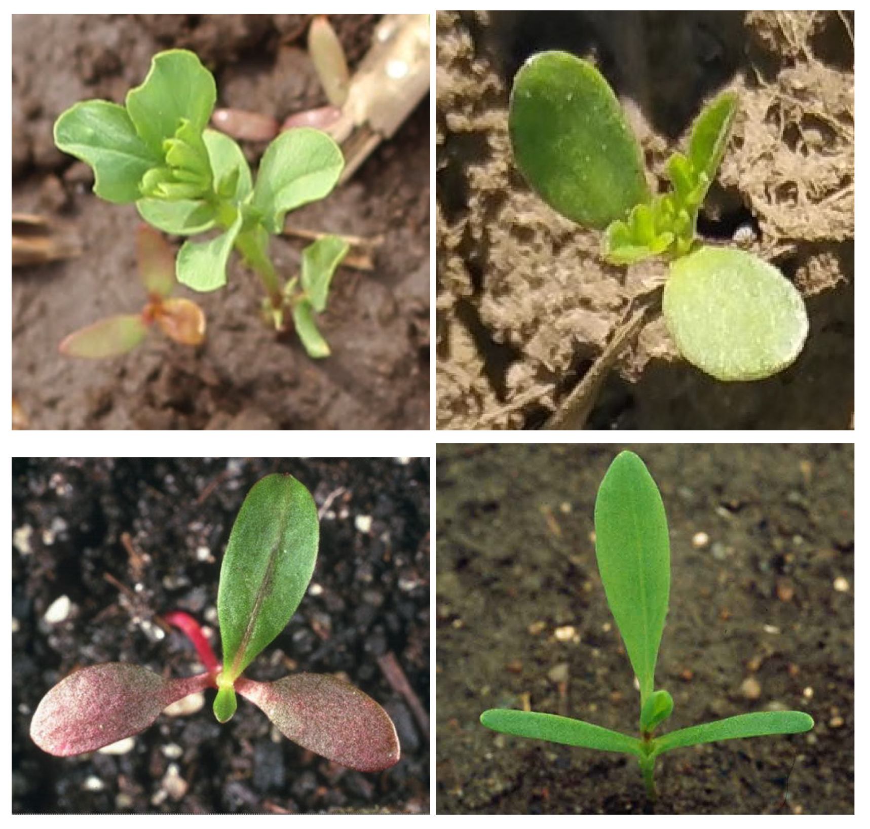
Figure 2.
Spatial distribution of sampling points for integrated data collection across the 3.40-hectare lentil field, including outside points measurements from drone imagery analysis (n=1,651), soil electrical conductivity measurements (blue points) at 75 cm and 150 cm depths using EM38-MK2 sensor (n=1,899 each), and NDVI grid samples from Sentinel-2 satellite imagery (n=200). The dark boundary line delineates the field perimeter used for spatial analysis and management zone delineation.
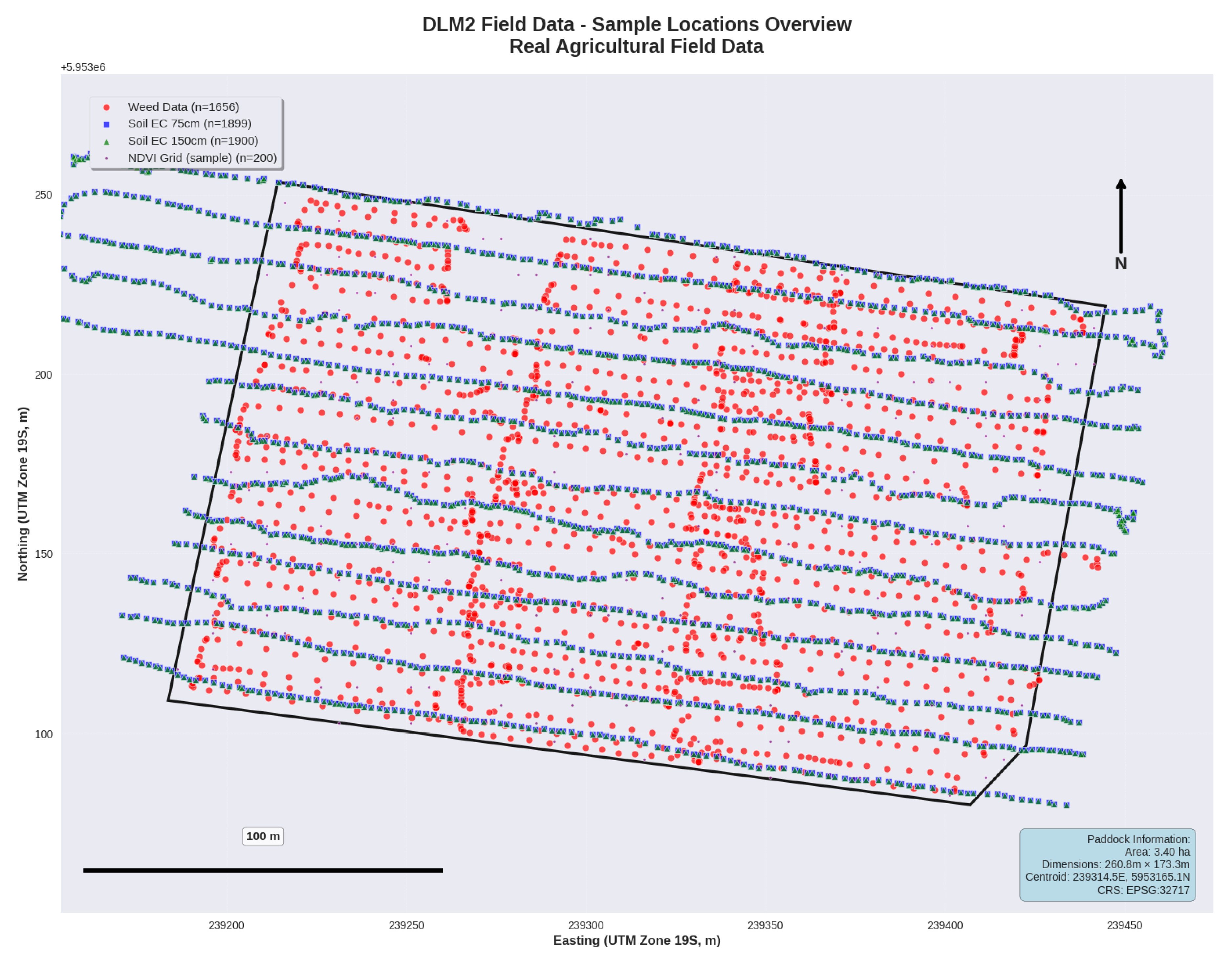
Figure 3.
Unified 5 by 5 m grid obtained from interpolated variables.
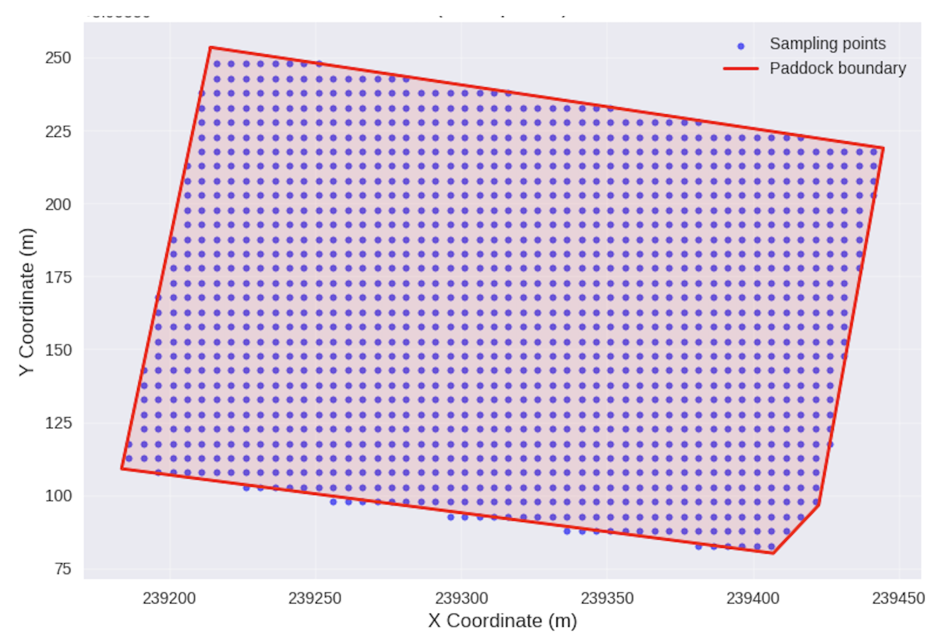
Figure 4.
YOLOv11 training performance across 50 epochs showing loss functions and evaluation metrics. Top row: training losses for bounding box regression (box_loss), classification (cls_loss), and distribution focal loss (dfl_loss), with corresponding validation losses below each. Bottom row: performance metrics including precision, recall, mean Average Precision at IoU threshold 0.5 (mAP50), and mAP at IoU thresholds 0.5:0.95 (mAP50-95). Blue lines represent actual values, while orange dotted lines indicate smoothed trends. The model achieved convergence by epoch 25 with stable performance metrics suitable for agricultural deployment.
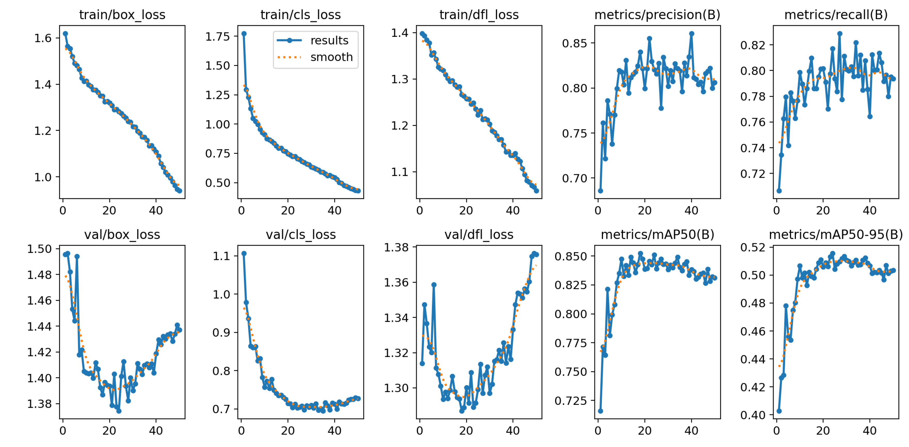
Figure 5.
F1-confidence curves for YOLOv11 model performance across target species. Individual curves show species-specific detection performance: LENCU (Lens culinaris, orange), AMBEL (Ambrosia artemisiifolia, blue), POLPE (Polygonum persicaria, red), and POLAV (P. aviculare, green). The thick blue line represents overall model performance across all classes, achieving an optimal F1-score of 0.82 at a confidence threshold of 0.339. Peak performance varies by species, with LENCU showing the highest discrimination capability (F1 = 0.87) and POLAV exhibiting reduced detection efficiency (F1 = 0.69), reflecting morphological and size differences among target classes.
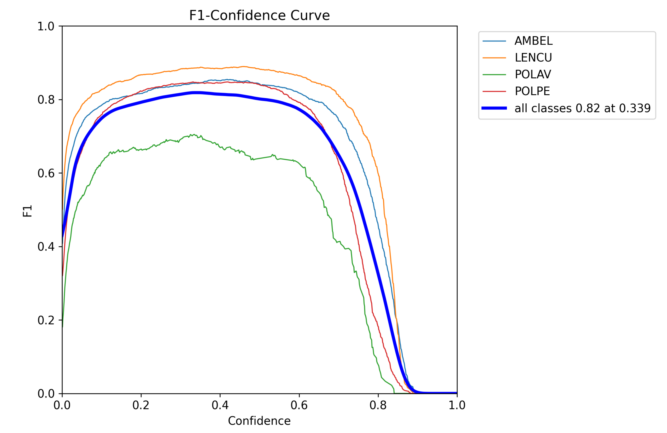
Figure 6.
Normalized confusion matrix for YOLOv11 species classification performance. The matrix shows true class labels (vertical axis) versus predicted classes (horizontal axis) with classification accuracies expressed as proportions. Diagonal elements represent correct classifications: LENCU (0.95), AMBEL (0.88), POLPE (0.85), and POLAV (0.73). Off-diagonal elements indicate misclassification patterns, with background confusion being the primary source of classification errors rather than inter-species confusion. Dark blue indicates high accuracy, while light blue represents lower classification rates.
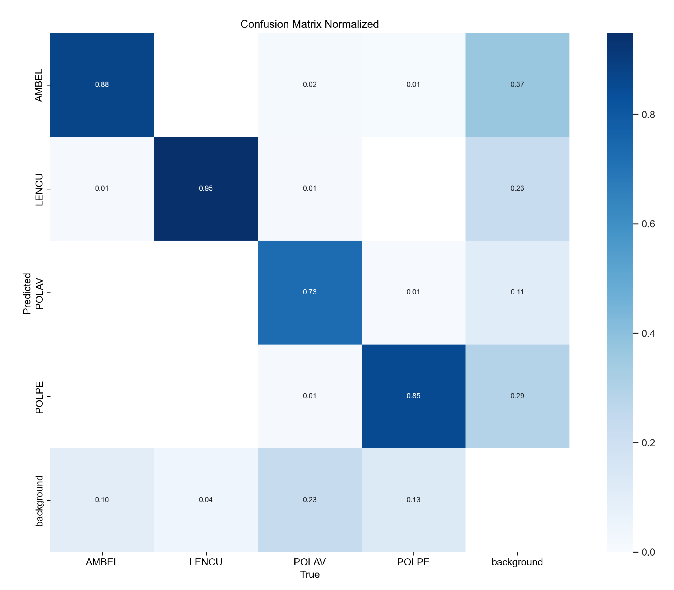
Figure 7.
Spatial distribution of drone image capture locations (red points) across the 3.42-hectare lentil field showing the systematic grid sampling pattern used for YOLOv11+SAHI model deployment. The grid-based approach ensured complete field coverage with 1,651 individual image captures, providing a comprehensive spatial representation for subsequent AI-based plant detection and geostatistical analysis integration.
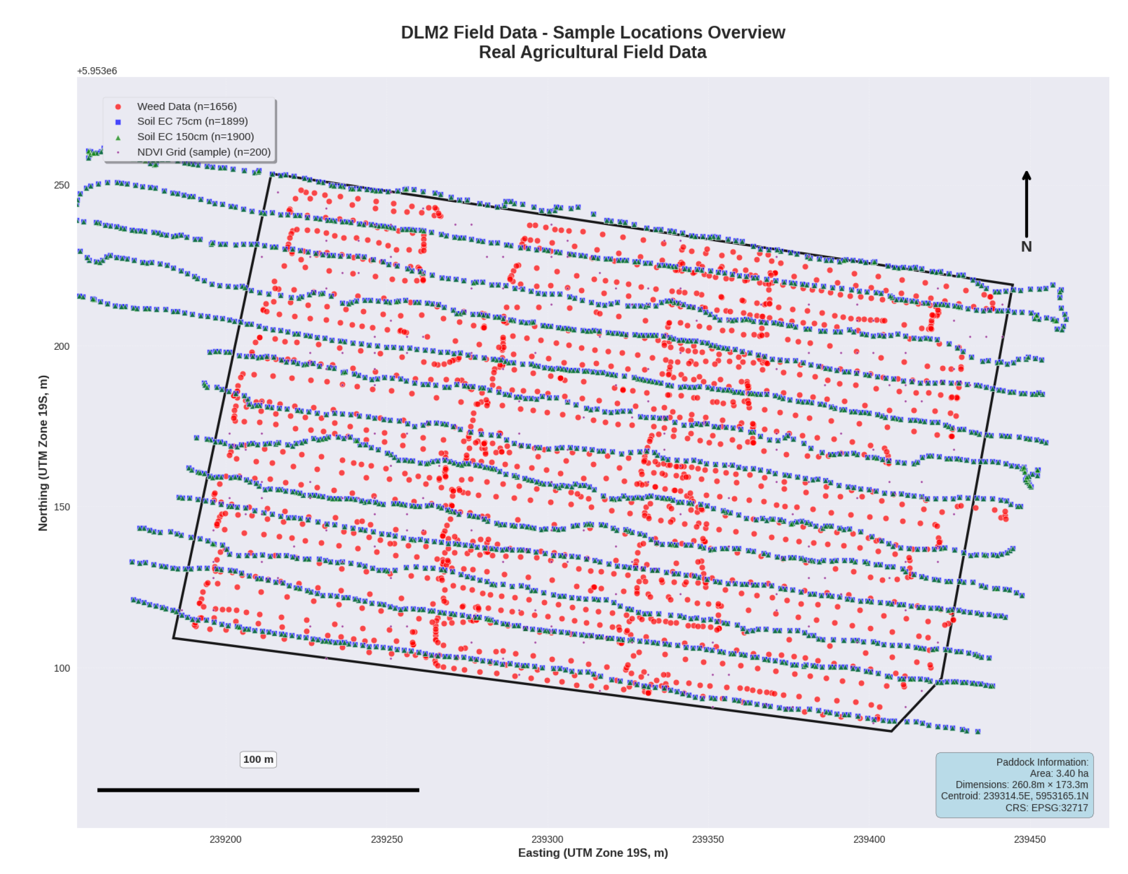
Figure 8.
YOLOv11+SAHI inference results showing species-specific detection performance in a representative field section with moderate to high weed density. Individual seedlings are detected with species-specific bounding boxes and confidence scores: magenta = AMBEL (Ambrosia artemisiifolia, 492 detections), blue = LENCU (Lens culinaris, 313 detections), orange = POLAV (P. aviculare, 1 detection), and yellow = POLPE (P. persicaria, 8 detections). Confidence scores (0.30-0.80 range) are displayed above each detection, demonstrating the model’s discriminative capability across varying plant sizes and orientations. The highlighted white rectangular area shows a zoomed region illustrating detection precision at individual seedling level, with successful identification of both crop and weed species in complex field conditions. Total plant count for this image section: 814 individual seedlings detected across four species.
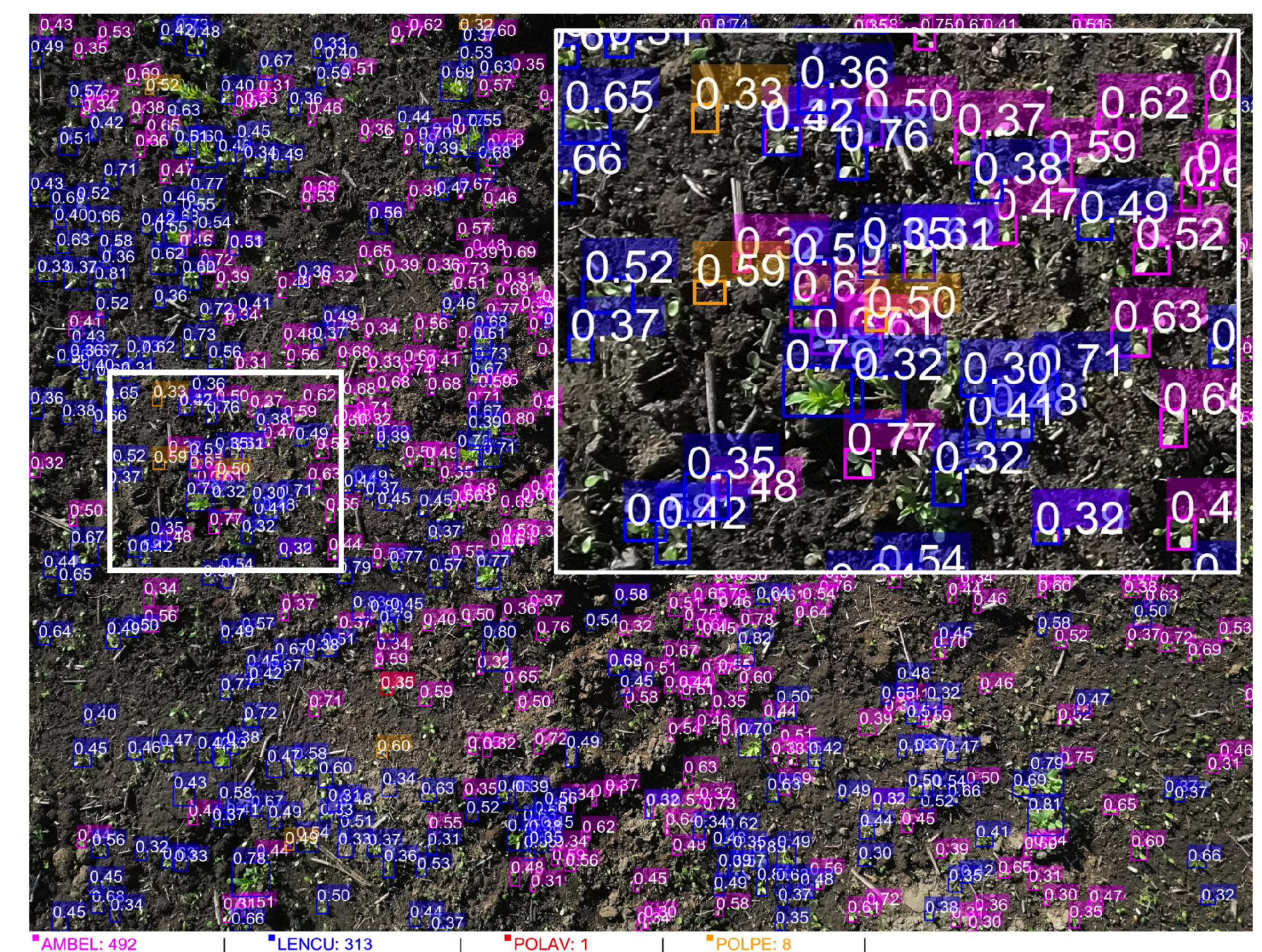
Figure 9.
YOLOv11+SAHI inference results in a low weed pressure scenario demonstrating accurate species-specific detection and crop-weed discrimination. Individual seedlings are detected with species-specific bounding boxes and confidence scores: blue = LENCU (\textit{Lens culinaris}, 39 detections), magenta = AMBEL (\textit{Ambrosia artemisiifolia}, 6 detections), yellow = POLPE (\textit{P. persicaria}, 1 detection), and orange = POLAV (\textit{P. aviculare}, 0 detections). High confidence scores (0.30-0.84 range) demonstrate reliable detection performance even under sparse plant density conditions. The clear soil background and well-spaced individual seedlings illustrate the framework’s capability to maintain detection accuracy in low-density scenarios typical of effective early-season weed management areas. Total plant count: 46 individual seedlings with a crop-to-weed ratio of 5.6:1, indicating successful crop establishment with minimal weed competition.
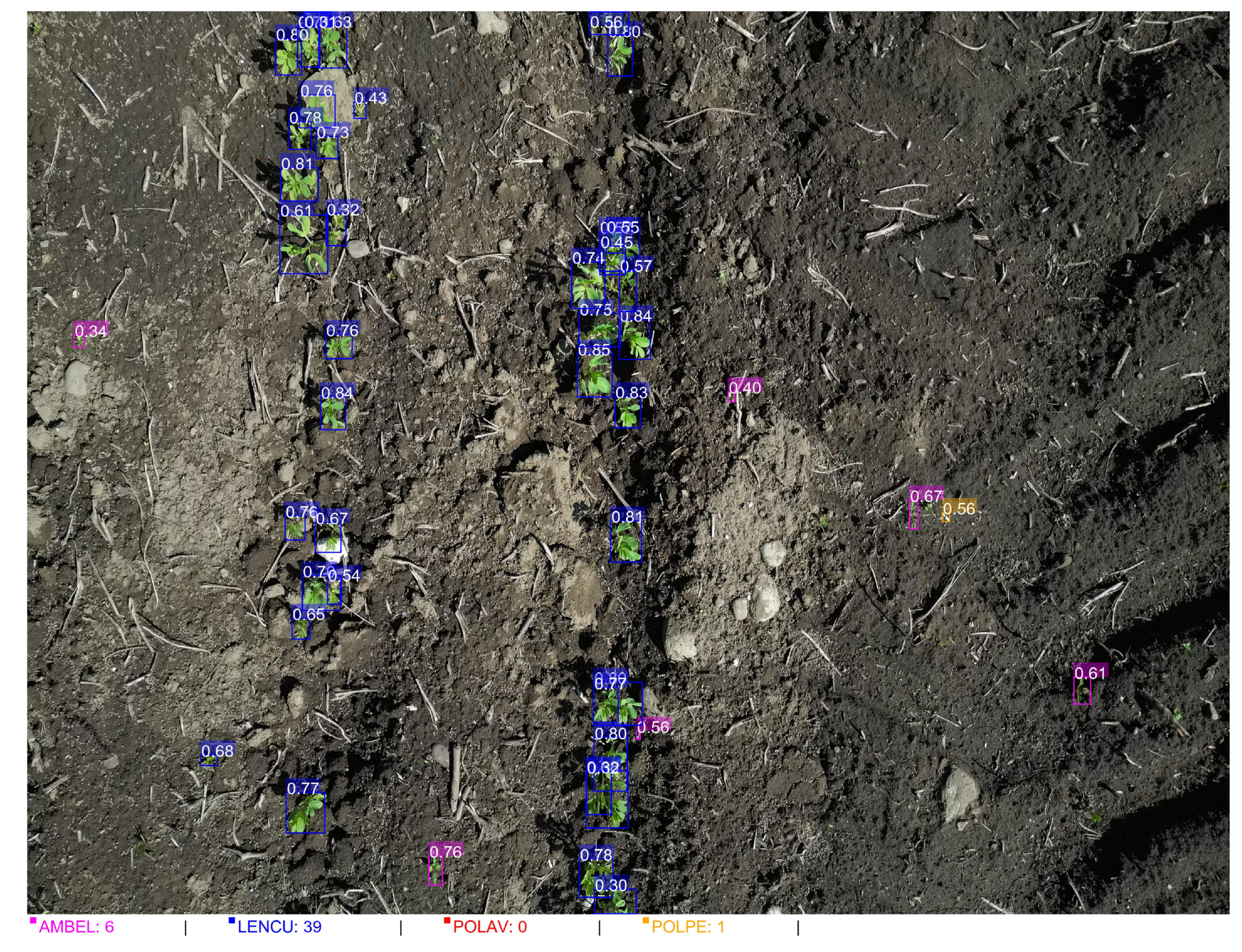
Figure 10.
Distribution plots for representative raw variables to be interpolated.
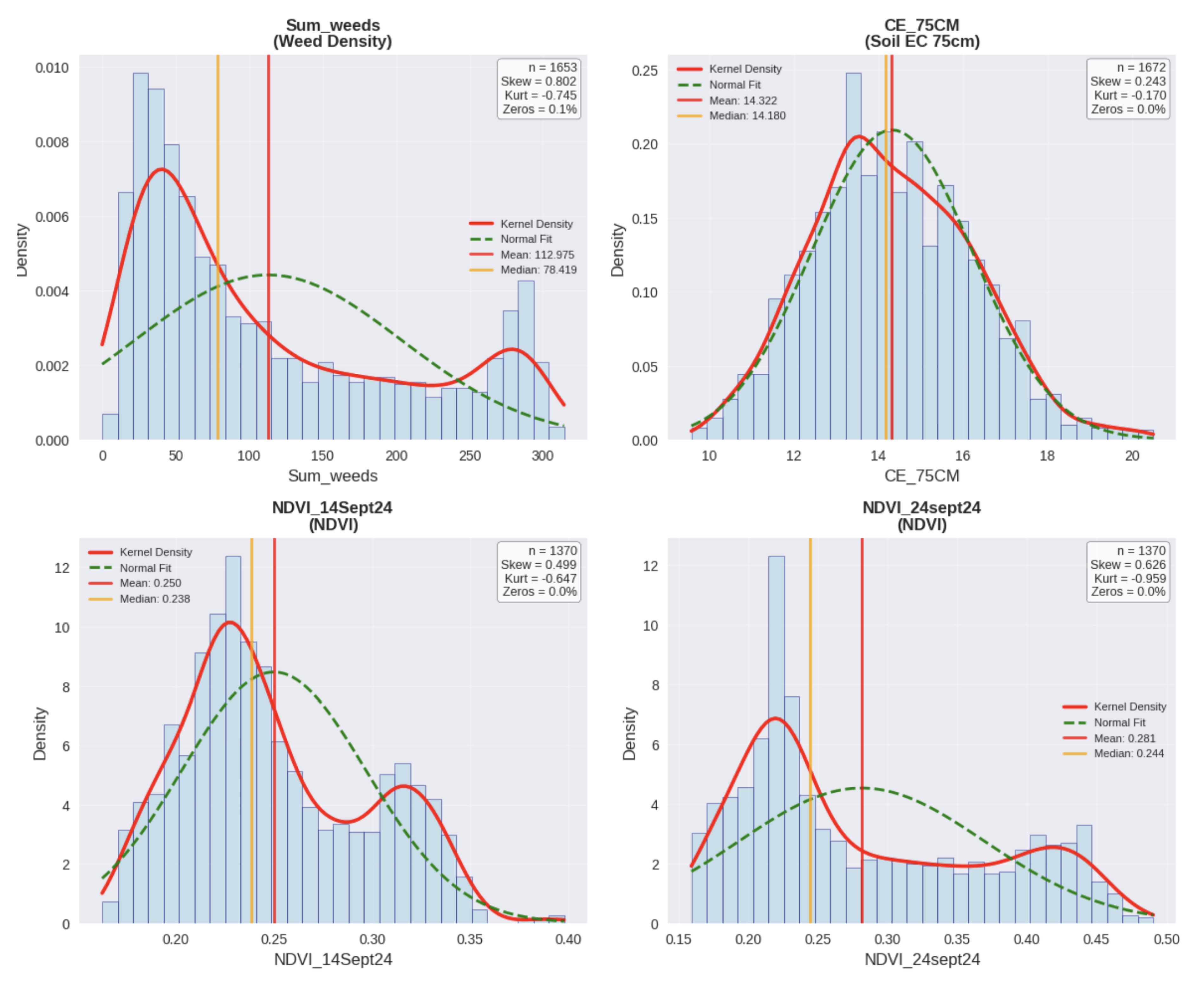
Figure 11.
Correlation matrix for the analyzed variables

Figure 12.
Spatial distribution maps for Ambrosia artemisiifolia (AMBEL). (a) seedling density (plants per sqm); (b) Local Indicator of Spatial Association (LISA) (c) Moran’s I Index; (d) LISA significance map
Figure 12.
Spatial distribution maps for Ambrosia artemisiifolia (AMBEL). (a) seedling density (plants per sqm); (b) Local Indicator of Spatial Association (LISA) (c) Moran’s I Index; (d) LISA significance map
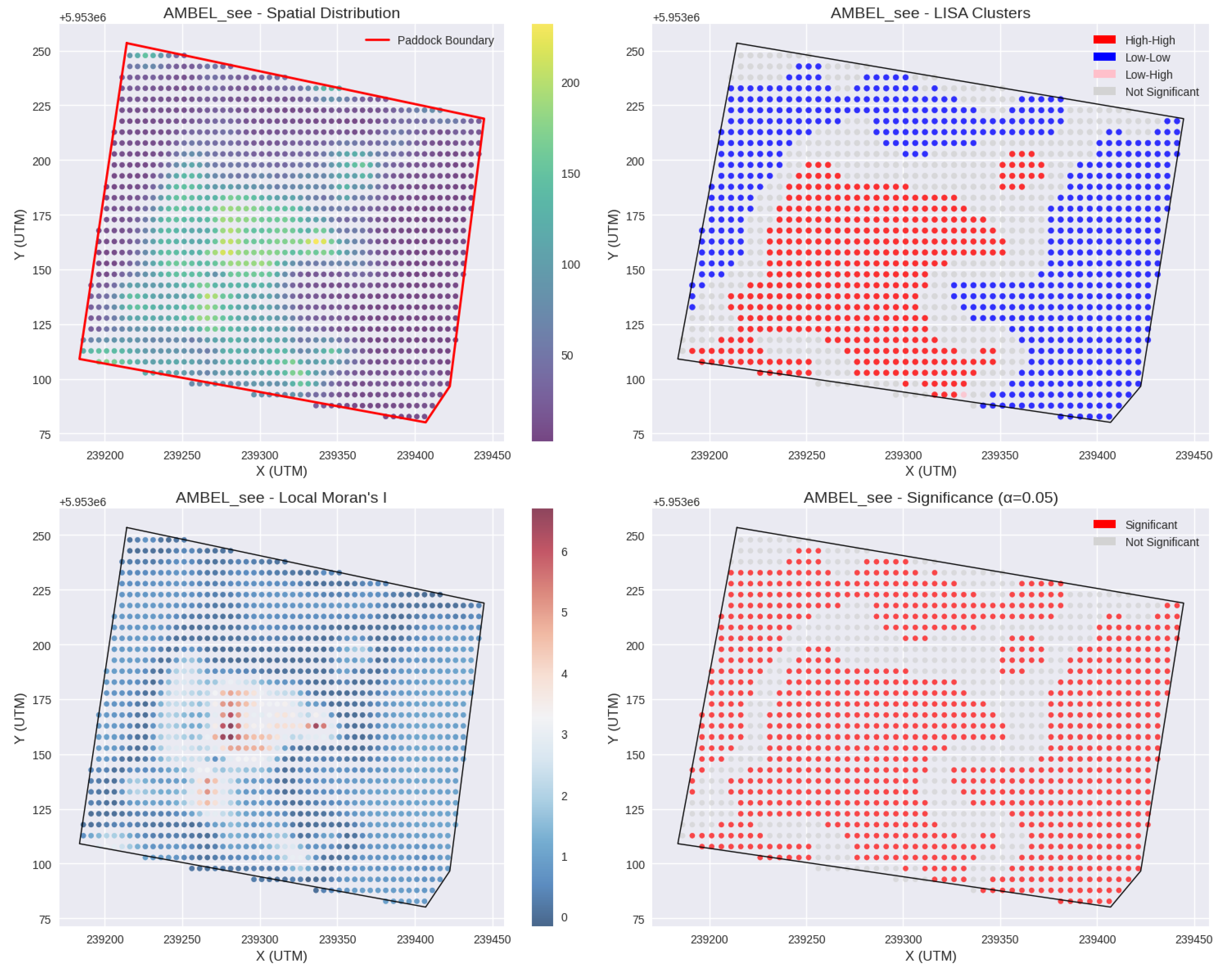
Figure 13.
Overlay map for AMBEL vs NDVI_14S, showing a strong positive co-location.
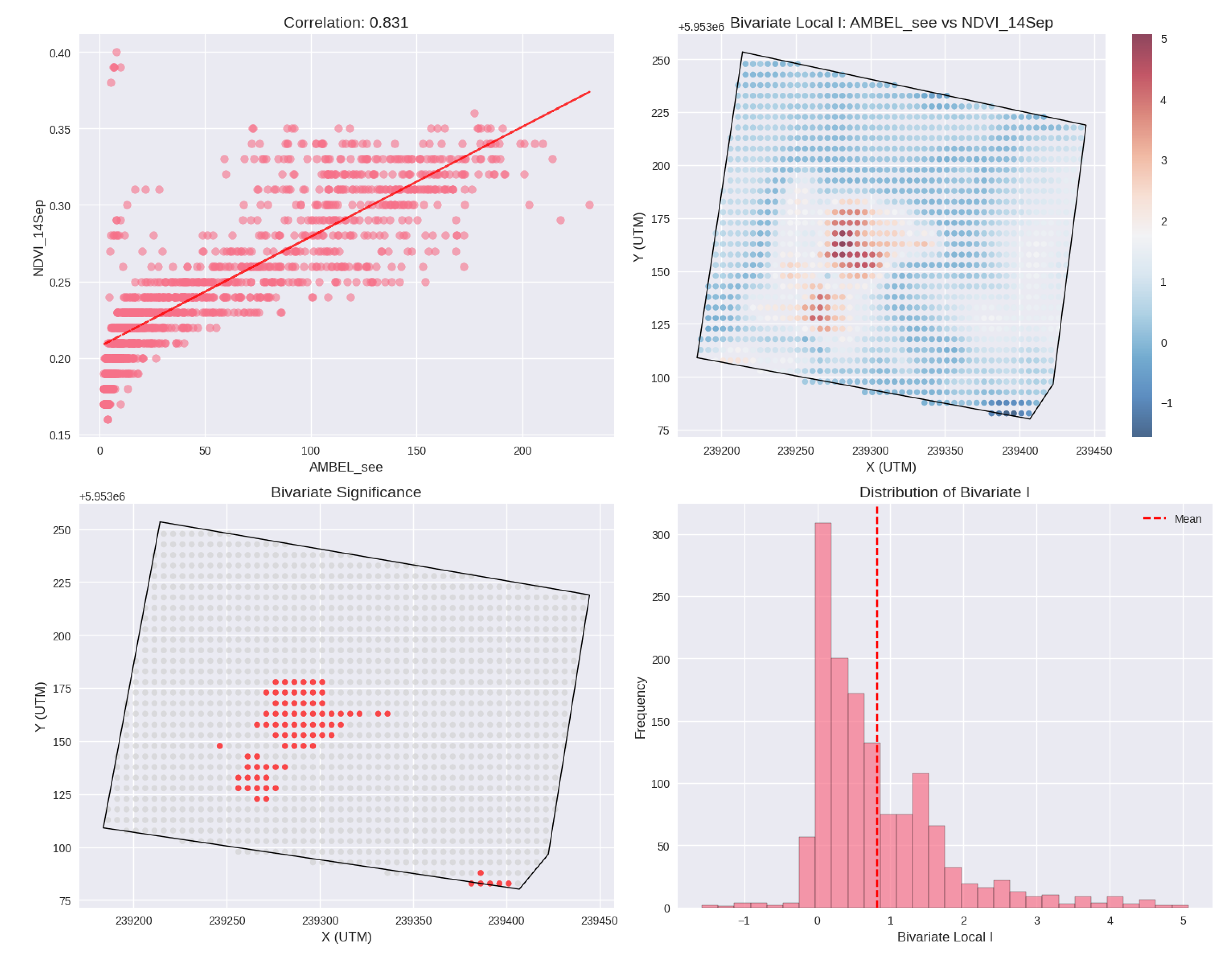
Figure 14.
Bivariate Local Indicators of Spatial Association (LISA) map showing co-location patterns between AMBEL density (plants m-2, represented by circles with brown color palette) and NDVI_14S values (background gradient in green to brown tones). The overlay reveals significant positive spatial associations between high weed density areas and vegetation vigor, indicating favorable microsites for Ambrosia artemisiifolia establishment.
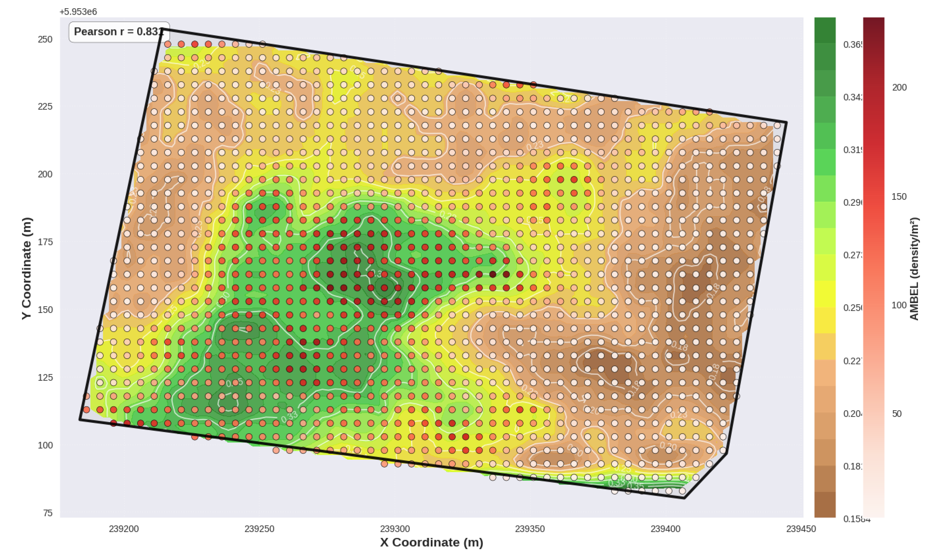
Figure 15.
Bivariate LISA analysis for AMBEL vs CE75, showing a moderate positive co-location
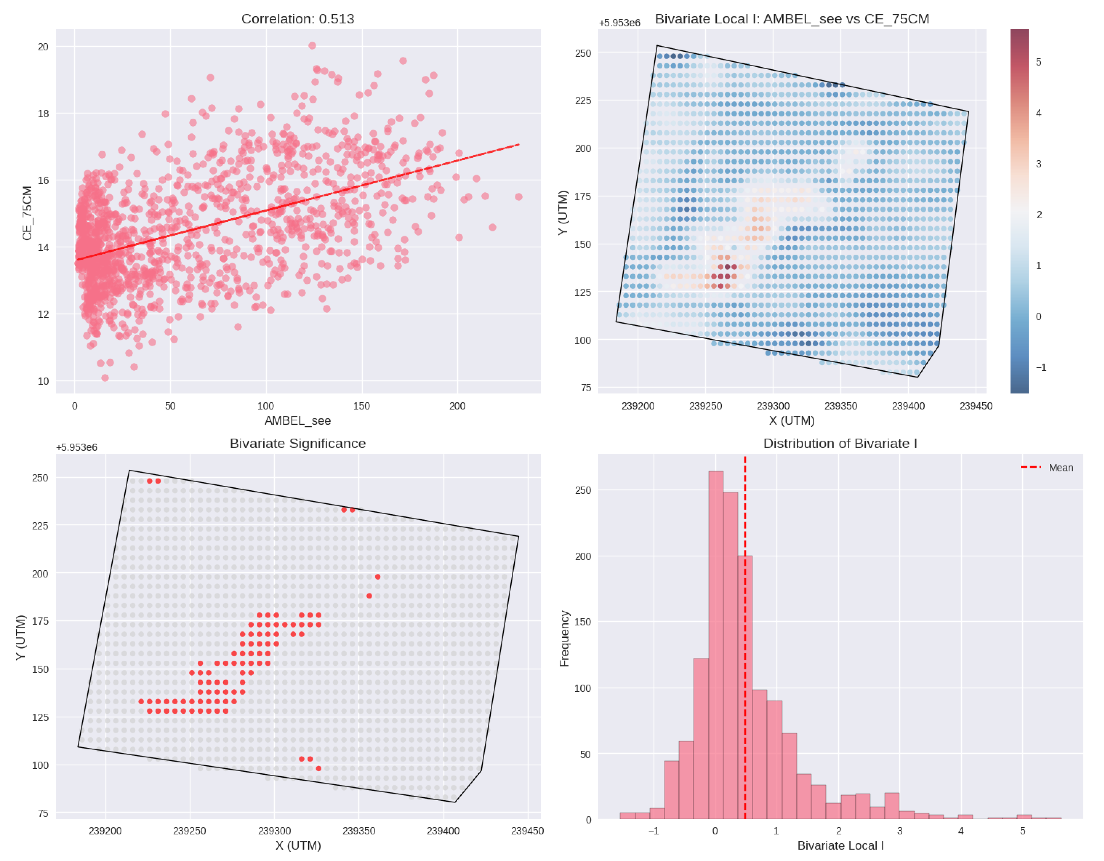
Figure 16.
Bivariate Local Indicators of Spatial Association (LISA) map showing co-location patterns between AMBEL density (plants m-2, represented by circles with brown color palette) and CE_75CM values (background gradient in yellow to blue tones). The overlay reveals moderate positive spatial associations between Ambrosia artemisiifolia density and shallow soil electrical conductivity, suggesting that areas with higher moisture retention and finer soil texture favor weed establishment.
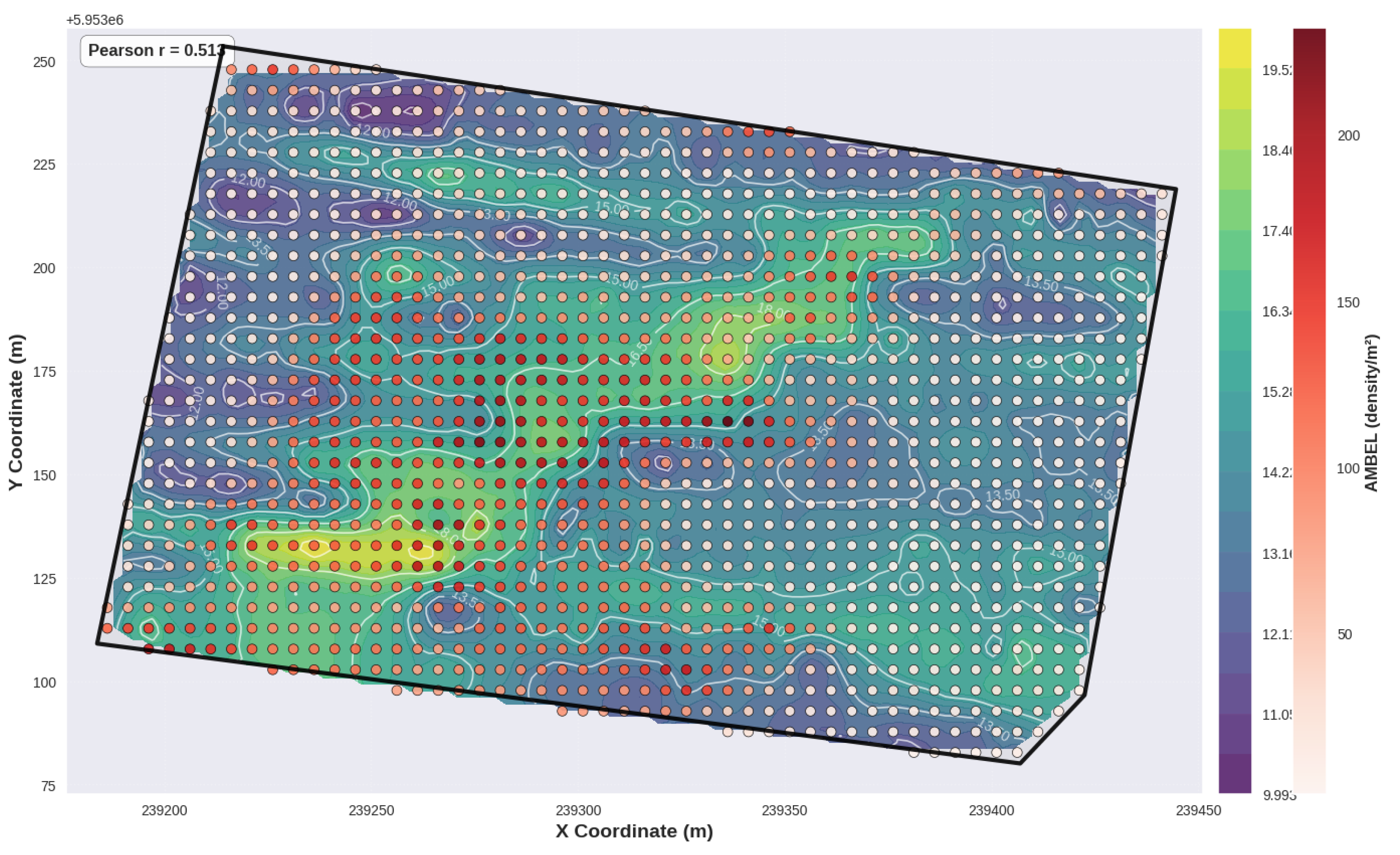
Figure 17.
Spatial analysis of weed community structure and competition patterns in the lentil field. (a) Dominant weed species distribution showing Ambrosia artemisiifolia (AMBEL) dominance across 1,331 grid points (96.8% of sampled area), with minimal Polygonum aviculare (POLAV) presence in 39 locations. (b) Weed competition zones using RGB color mixing to represent relative species proportions, where red intensity indicates AMBEL dominance, green represents POLPE presence, and blue shows POLAV distribution. Point size reflects total weed density per grid cell. (c) Weed-to-crop competition ratio interpolated surface, with green areas indicating crop dominance (low weed pressure), yellow zones showing balanced competition, and red regions representing high weed-to-crop ratios requiring intensive management. (d) Community cluster analysis revealing four distinct management zones based on species composition and density patterns, with Zone 1 (purple) showing highest AMBEL pressure (431.0 plants m-2), Zones 2–4 exhibiting moderate to low weed densities, and Zone 3 (teal) representing areas with significant POLPE co-occurrence (113.4 plants m-2).
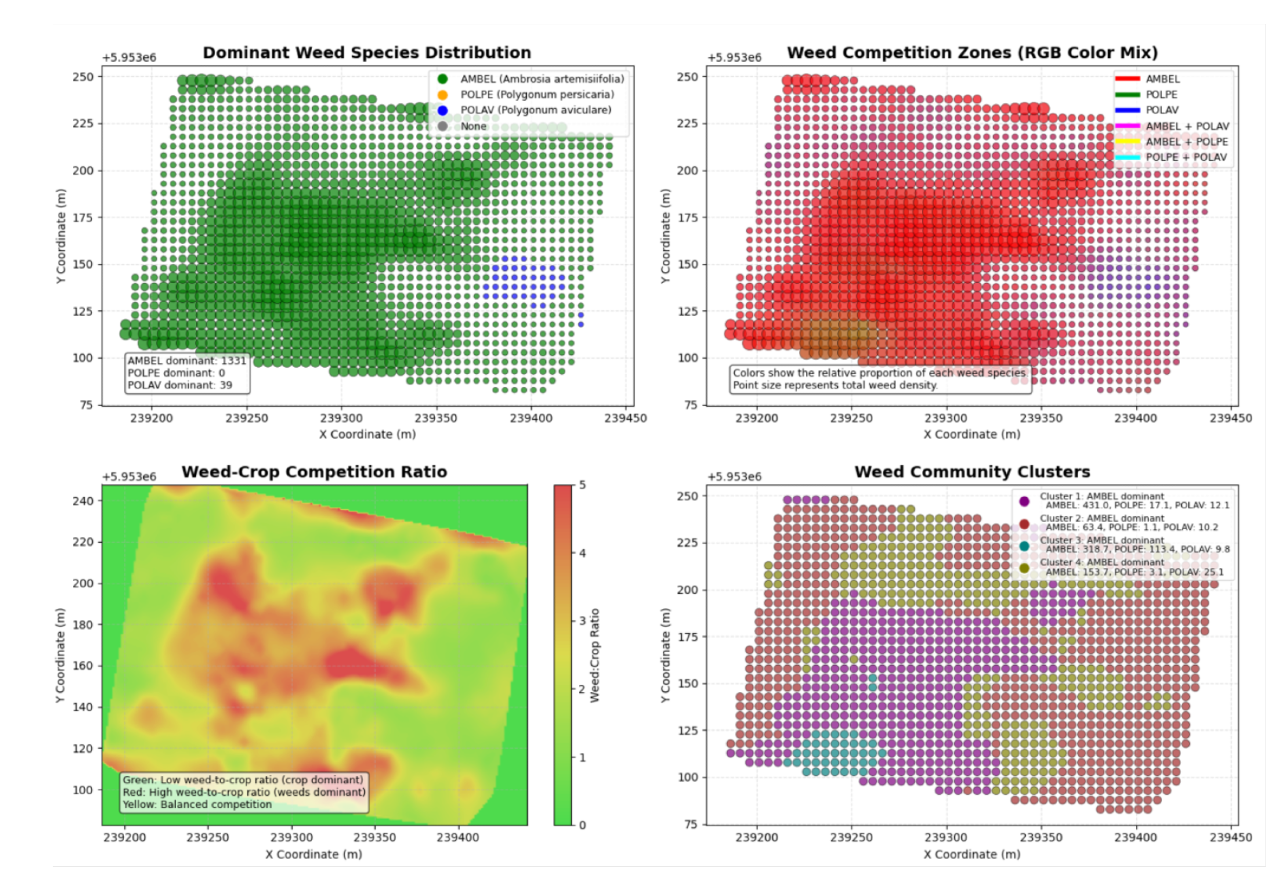

Table 1.
Climatic characteristics of the experimental site during the first eight years of crop rotation development.
Table 1.
Climatic characteristics of the experimental site during the first eight years of crop rotation development.
| Season | Mean Temperature (°C) | Precipitation (mm) | Evaporation (mm) |
|---|---|---|---|
| 2016 | 12.8 | 605 | 1023 |
| 2017 | 13.2 | 563 | 1041 |
| 2018 | 13.5 | 730 | 990 |
| 2019 | 13.4 | 632 | 994 |
| 2020 | 13.6 | 746 | 1077 |
| 2021 | 13.5 | 649 | 940 |
| 2022 | 13.2 | 920 | 966 |
| 2023 | 13.7 | 1209 | 925 |
Table 2.
Physical and hydric soil properties at the experimental site.
| Parameter | Value |
|---|---|
| Clay, % | 16.7 |
| Silt, % | 44.6 |
| Sand, % | 38.7 |
| Bulk density, g cm−3 | 1.00 |
| pH (soil:water 1:5) | 5.52 |
| Electrical conductivity, EC (dS m−1) | 0.11 |
Table 3.
Morphological characteristics of crop and weed seedlings during early development (BBCH 10–14).
Table 3.
Morphological characteristics of crop and weed seedlings during early development (BBCH 10–14).
| Species (EPPO) | BBCH Stage | Cotyledon Shape | First True Leaves |
|---|---|---|---|
| L. culinaris (Crop) | 12–14 | Hypogeal (not visible) | Pinnate, pubescent |
| A. artemisiifolia (AMBEL) | 10–14 | Spatulate, opposite | Deeply lobed, pubescent |
| P. persicaria (POLPE) | 10–12 | Lanceolate, narrow | Ovate, reddish midrib |
| P. aviculare (POLAV) | 10–12 | Linear-elliptical | Oblong, alternate |
Table 4.
Camera specifications and acquisition parameters for training dataset development.
| Parameter | Specification |
|---|---|
| Sensor | APS-C CMOS (22.3 × 14.9 mm) |
| Resolution | 18.0 MP (5184 × 3456 pixels) |
| Focal length | 18–55 mm (equivalent to 29–88 mm in 35mm format) |
| Aperture range | f/3.5–5.6 |
| ISO sensitivity | 100–400 (optimal conditions) |
| Shutter speed | 1/250–1/500 s |
| Image format | JPEG (Fine quality, sRGB color space) |
| Shooting height | 1.2 ± 0.1 m above crop canopy |
| Ground sampling distance | 0.48 ± 0.05 mm pixel−1 |
Table 5.
Descriptive statistics for weed densities, soil properties, and vegetation indices in the lentil field study area.
Table 5.
Descriptive statistics for weed densities, soil properties, and vegetation indices in the lentil field study area.
| Variable | N | Mean | SD | CV | Min | Max | Skewness |
|---|---|---|---|---|---|---|---|
| Weed Densities (plants m-2) | |||||||
| AMBEL1 | 1651 | 66.46 | 69.20 | 1.04 | 0.00 | 262.01 | 1.02 |
| LENCU2 | 1651 | 39.29 | 27.98 | 0.71 | 0.00 | 209.12 | 1.65 |
| POLPE3 | 1651 | 2.83 | 9.04 | 3.20 | 0.00 | 141.34 | 8.05 |
| POLAV4 | 1651 | 4.32 | 3.88 | 0.90 | 0.00 | 37.69 | 2.26 |
| Total weeds | 1651 | 113.09 | 90.41 | 0.80 | 0.00 | 314.29 | 0.80 |
| Soil Properties | |||||||
| CE_75CM (mS m-1) | 1608 | 14.35 | 1.91 | 0.13 | 9.57 | 20.51 | 0.24 |
| CE_150CM (mS m-1) | 1608 | 14.78 | 1.31 | 0.09 | 10.90 | 20.70 | 0.98 |
| Vegetation Indices | |||||||
| NDVI_14S | 1370 | 0.250 | 0.047 | 0.19 | 0.163 | 0.398 | 0.50 |
| NDVI_24S | 1370 | 0.281 | 0.088 | 0.31 | 0.159 | 0.491 | 0.63 |
| NDVI_diff | 1370 | 0.031 | 0.045 | 1.43 | -0.044 | 0.168 | 0.61 |
CV = Coefficient of Variation; NDVI_diff = NDVI_24S - NDVI_14S. 1Ambrosia artemisiifolia; 2Lens culinaris; 3Polygonum persicaria; 4Polygonum aviculare. Zero values: AMBEL (0.12%), LENCU (0.12%), POLPE (39.9%), POLAV (3.1%).
Table 6.
Semivariogram model parameters and spatial dependence characteristics for interpolated variables.
Table 6.
Semivariogram model parameters and spatial dependence characteristics for interpolated variables.
| Variable | Model | Nugget | Sill | Range (m) | Nugget/Sill | Spatial Dependence | AIC |
|---|---|---|---|---|---|---|---|
| CE_75 | Exponential | 0.85 | 2.94 | 45.2 | 0.29 | Moderate | -1847.3 |
| CE_150 | Exponential | 0.32 | 1.48 | 52.8 | 0.22 | Strong | -2156.8 |
| NDVI_14S | Spherical | 0.00 | 0.0022 | 38.7 | 0.00 | Very Strong | -4821.2 |
| NDVI_24S | Spherical | 0.15 | 0.0075 | 41.3 | 0.02 | Very Strong | -3642.1 |
| LENCU | Spherical | 185.2 | 502.3 | 35.4 | 0.37 | Moderate | 12847.9 |
| Sum_weeds | Spherical | 1456.8 | 8156.2 | 42.8 | 0.18 | Strong | 15234.7 |
| POLPE | Exponential | 23.1 | 40.4 | 28.9 | 0.57 | Weak | 9876.4 |
| POLAV | Gaussian | 4.8 | 5.2 | 19.3 | 0.92 | Very Weak | 6543.2 |
Spatial dependence classification: Very Strong (<0.25), Strong (0.25–0.50), Moderate (0.50–0.75), Weak/Very Weak (>0.75). AIC = Akaike Information Criterion (lower values indicate better fit).
Table 7.
Leave-one-out cross-validation results for ordinary kriging interpolation of environmental and biological variables.
Table 7.
Leave-one-out cross-validation results for ordinary kriging interpolation of environmental and biological variables.
| Variable | RMSE | R² | Slope | Intercept | Units | Performance |
|---|---|---|---|---|---|---|
| 0.006 | 0.996 | 1.011 | -0.003 | – | Excellent | |
| 0.516 | 0.923 | 0.995 | 0.070 | mS m-1 | Excellent | |
| 0.447 | 0.862 | 1.029 | -0.422 | mS m-1 | Very Good | |
| 39.593 | 0.810 | 1.052 | -5.971 | plants m-2 | Very Good | |
| AMBEL | 32.529 | 0.782 | 1.065 | -4.264 | plants m-2 | Good |
| LENCU | 17.506 | 0.609 | 1.033 | -1.378 | plants m-2 | Good |
| POLPE | 6.359 | 0.509 | 1.082 | -0.185 | plants m-2 | Moderate |
| POLAV | 3.037 | 0.390 | 1.067 | -0.304 | plants m-2 | Poor |
Performance categories: Excellent (R² ≥ 0.9), Very Good (0.8–0.9), Good (0.6–0.8), Moderate (0.4–0.6), Poor (< 0.4).
Table 8.
Global and local spatial autocorrelation results for key variables using distance-based spatial weights (30 m threshold).
Table 8.
Global and local spatial autocorrelation results for key variables using distance-based spatial weights (30 m threshold).
| Variable | Global Moran’s I | p-value | Significant Clusters | Coverage (%) | Primary Cluster Type |
|---|---|---|---|---|---|
| NDVI_24S | 0.795 | <0.001 | 925 | 67.5 | Low-Low (39.9%) |
| NDVI_14S | 0.745 | <0.001 | 798 | 58.2 | Low-Low (31.5%) |
| Diff_NDVI | 0.764 | <0.001 | 972 | 70.9 | Low-Low (42.0%) |
| LENCU | 0.770 | <0.001 | 831 | 60.7 | Low-Low (35.8%) |
| AMBEL | 0.667 | <0.001 | 992 | 72.4 | Low-Low (43.2%) |
| CE_150 | 0.591 | <0.001 | 806 | 58.8 | Low-Low (35.9%) |
| CE_75 | 0.452 | <0.001 | 674 | 49.2 | Low-Low (27.4%) |
| POLPE | 0.518 | <0.001 | 809 | 59.1 | Low-Low (50.1%) |
| POLAV | 0.289 | <0.001 | 652 | 47.6 | Low-Low (27.8%) |
Spatial weights based on 30 m distance threshold (mean 96.6 neighbors per point). Coverage = percentage of points with statistically significant local clustering (p < 0.05).
Table 9.
Bivariate Local Indicators of Spatial Association (LISA) results for key variable pairs.
| Variable Pair | Global r | Spatial r | Significant (%) | Positive | Negative |
|---|---|---|---|---|---|
| AMBEL ↔ NDVI_14S | 0.831 | 0.818 | 86.4 | 1086 | 98 |
| LENCU ↔ NDVI_14S | 0.837 | 0.871 | 86.3 | 1082 | 100 |
| Total_Weeds ↔ NDVI_14S | 0.846 | 0.837 | 86.3 | 1083 | 99 |
| AMBEL ↔ LENCU | 0.784 | 0.759 | 87.6 | 1086 | 114 |
| POLPE ↔ LENCU | 0.608 | 0.621 | 87.7 | 1015 | 186 |
| CE_75 ↔ Diff_NDVI | 0.542 | 0.515 | 90.4 | 864 | 374 |
| CE_150 ↔ NDVI_24S | 0.536 | 0.513 | 89.6 | 811 | 417 |
| AMBEL ↔ CE_75 | 0.513 | 0.633 | 74.3 | 845 | 173 |
| POLPE ↔ CE_150 | 0.584 | 0.650 | 74.9 | 806 | 220 |
| CWR ↔ NDVI_14S | -0.611 | -0.593 | 86.7 | 280 | 908 |
Global r = Pearson correlation coefficient; Spatial r = spatial cross-correlation. Significant (%) = percentage of spatially significant local associations (p < 0.05). Positive/Negative = number of significant positive/negative local associations. CWR = Crop-to-Weed Ratio.
Table 10.
Species-based management zone characteristics derived from fuzzy clustering analysis.
| Zone | Area (ha) | Points (n) | Priority | Membership |
|---|---|---|---|---|
| Zone 1 | 0.70 | 280 | Medium | 0.76 |
| Zone 2 | 1.00 | 400 | Critical | 0.82 |
| Zone 3 | 0.09 | 36 | Critical | 0.68 |
| Zone 4 | 1.63 | 654 | Low | 0.87 |
Membership = mean fuzzy membership coefficient for zone assignment. Priority levels: Critical (immediate intervention), Medium (targeted management), Low (maintenance). AMBEL = Ambrosia artemisiifolia (primary target species).
Disclaimer/Publisher’s Note: The statements, opinions and data contained in all publications are solely those of the individual author(s) and contributor(s) and not of MDPI and/or the editor(s). MDPI and/or the editor(s) disclaim responsibility for any injury to people or property resulting from any ideas, methods, instructions or products referred to in the content. |
© 2025 by the authors. Licensee MDPI, Basel, Switzerland. This article is an open access article distributed under the terms and conditions of the Creative Commons Attribution (CC BY) license (http://creativecommons.org/licenses/by/4.0/).
Copyright: This open access article is published under a Creative Commons CC BY 4.0 license, which permit the free download, distribution, and reuse, provided that the author and preprint are cited in any reuse.


