
Submitted:
19 February 2025
Posted:
20 February 2025
You are already at the latest version
Abstract
This study presents the evaluation of tools for weed analysis and management to support agroecological practices in organic farming, emphasizing agriculture digitalization and remote sensing. The main aim was to provide techniques for monitoring and prediction of weed spread using multispectral satellite and drone data, without the use of chemical inputs. Key findings indicate that VV and VH channels of Sentinel-1 and B2, B3, B4 and B8 channels of Sentinel-2 are not different regarding tillage, herbicide use, or sowing den-sity. However, RE and NIR channels of drone detected significant variations and proved effectiveness for weediness monitoring. The NIR channel is sensitive to agrotechnical factors such as cultivation type, making it valuable for field monitoring. Correlation and regression analyses revealed that B2, B3, B8 channels of Sentinel-2 and RE and NIR drone channels are the most reliable for predicting weed levels. Conversely, Sentinel-1 showed limited predictive utility. Random effect models confirmed that Sentinel-2 and drone channels can accurately account for site characteristics and timing of weed proliferation. Taken together these tools provide effective organic weed monitoring systems, enabling rapid identification of problem areas and adjustments in agronomic practices.
Keywords:
Agroecological farming
; Digitalization
; Drone
; Herbicide
; Organic agriculture
; Sentinel
; Weediness.
1. Introduction
Effective weed management is an important component of sustainable agricultural development in modern organic farming [1]. Organic production requires strong reduction or complete avoidance of the use of chemical herbicides, that stimulates development of alternative, environmentally safe methods of weed control [2,3,4,5]. The use of remote sensing (RS) data in precision agriculture is an important tool in modern agronomic management. Using RS technologies and geospatial data processing, it becomes possible to conduct accurate monitoring of the state of crops. Such analysis of images from Sentinel-1 and Sentinel-2 satellites and data from drones opens new opportunities for monitoring vegetation, including the assessment of the weediness [6].
RS data might be also used to identify areas with extensive weediness and analyze the effectiveness of herbicide-free agrotechnical methods. Remote sensing is the basis of modern approaches [7,8]. The use of spectral data from satellites or drones allows the analysis of light reflectance by vegetation in near-infrared (NIR) and mid-infrared (MIR) spectral ranges. In addition, the distribution of spectral reflectance can serve as useful indicator of different types of vegetation, including weeds [9,10,11].
The use of vegetation indices such as Normalized Difference Vegetation Index (NDVI), Soil-Adjusted Vegetation Index (SAVI) and Green Normalized Difference Vegetation Index (GNDVI) showed high efficiency in separating weeds from crops [12,13,14,15,16]. Recent advances in machine learning and artificial intelligence have significantly improved the accuracy of weed identification [17,18]. Algorithms such as Random Forest, Support Vector Machines (SVM) and neural networks are effectively used to analyze large amounts of RS data [18,19,20,21].
Maize is extensively used in such type of studies because it is one of the key agricultural crops where accurate determination of weed infestation level is critical to ensure high yields. According to earlier studies, the spectral properties of weeds are significantly different from those of maize, which allows effective RS using for their identification [10,22,23]. The use of unmanned aerial vehicles (UAVs) and satellite imagery combined with high-precision indices allows for the assessment of weed infestation levels over large areas with minimal cost [24,25,26].
Organic production of maize requires a tool that helps predict weed levels based on historical data. The model, which includes the coefficient of weediness such as integrated indicator that considers the density and height of grass, broadleaf, and root weeds, can be the basis for planning agrotechnical measures. This makes possible to evaluate the effectiveness of weed control measures and to improve management systems in agroecological farming. Thus, the goal of present study was to develop and substantiate new approaches to weed management based on agriculture digitalization and RS technologies. The study was designed in the way to evaluate the possibilities of analyzing the state of weeding using multispectral images from satellites and drones, to identify key factors affecting the level of weeding, and to create a model that will allow effective monitoring and forecasting of weeding without the use of chemicals.
The outcomes of using remote sensing and drone data may be very different, though, depending on the crop being analyzed, the processing technologies, the density of the plantation, and other technological factors. Therefore, we elucidated the potential applications of Sentinel-1, Sentinel-2, and drone images taken at different spectral channels in determining the extent of weed infestation in areas with varying plowing methods, sowing density, and natural protection, among other factors.
2. Materials and Methods
Key characteristics of experimental field. The experimental plot was a part of larger the experimental field of the Polissia National University (N 50°26′; E 28°42). The site has predominantly Gleic Albic Luvisol (Endoclayic, Cutanic, Differentic, Katogleyic, Ochric type of soil according to WRB (2022).
Weather conditions significantly affect the quality of space or drone shooting and shooting from drones, it should be noted that the weather of research area is moderately continental with humid conditions. The average annual air temperature is about 7–8 °C, and the average temperature in January is about 5 °C. The summer temperature usually ranges between 18–20 °C. The amount of precipitation varies between 600–700 mm per year, with the most part falling in the summer period. The relative humidity of the air is significantly raised.
Analysis of variance is used to evaluate the effects of factors F1, F2, F3, and their interactions. Experiment was tested in three replications to minimize experimental error and improve result validity.
Plot of about 1 hectare was divided into 12 experimental plots with three replications (Figure 1). The research employs a factorial experimental design where F1, F2, F3 were combined. Еach combination of F1 × F2 × F3 was implemented in three replicates. The study explored the impact of the following factors: F1 - tillage systems: S1- deep soil plowing on 18–20 cm (standard), S2 – soil disking on 10–12 cm (AES), S3 – soil milling on 5–7 cm (AES); F2 – sowing density: A1 – 1.1 sowing units/ha (standard); A2 – 1.3 sowing units/ha (AES); F3 - herbicide application: H1 – herbicide application (standard); H2 - herbicide nonapplication (AES).
Data were collected with a frequency of one week using each source. During field research, the parameters of main crops, cereal weeds, broadleaf, and short-leaved weeds were measured by height and density for each plot.
To conduct aviation research copter-type DJI Mavic 3M drone was used with a multispectral camera of the following characteristics: image sensor – 1/2.8-inch CMOS, effective pixels: 5 Mn; Lens – FOV: 73.91° (61.2° x 48.10°); equivalent focal length – 25 mm; aperture – f/2.0; fixed focus; image format – TIFF; video resolution – H.264 FHD: 1920 x 1080@30 fps.
Images were obtained in the following spectral ranges based on the results from aerial photography: Green (G): 560 ± 16 nm; Red (R): 650 ± 16 nm; Red Edge (RE): 730 ± 16 nm; Near infrared range (NIR): 860 ± 26 nm. We determined the average values of radiation intensity in the specified spectral ranges, made calculations, and determined the average values of the NDVI vegetation index for each site over a five-week time interval during the geoinformation analysis of the obtained images.
Space research was conducted using data received from the Sentinel-1 and Sentinel-2 spacecraft. During Sentinel-1 measurements, space images were obtained in the radio wave range in the IWS mode with a resolution of 5 x 5 m, a bandwidth of 20 x 20 km with VV and VH polarization. As a result of data processing, the average values of the radiation intensity for the middle of each section were determined.
The reception of images from the Sentinel-2 optical-electronic observation spacecraft was carried out in the Band 2 (Blue) spectral ranges of 490 nm; Band 3 (Green) 560 nm; Band 4 (Red) 665 nm; Band 8 (NIR) 842 nm. The processing of the data from the space shooting was carried out according to the methodology like the processing of the data from the aerophotography by spectral channels with the determination of the vegetation index NDVI.
Database description. To effectively conduct the experiment, we formed a panel database that incorporated the results of physical examinations of plants and soil, data from the Sentinel-1 and Sentinel-2 satellites, and indicators from a drone. We collected data for five time points at each experimental site. This ensures the two-dimensionality of the data, enabling the analysis of the object individual features and their changes over time. Additionally, we ensured the stability of the sample when forming the panel database. Observation took place in the same areas, which do not change over time in terms of size and type of observation.
The object of the sample was 36 plots, which were formed from one experimental field where maize was sown. The database formation process provides the sample depth, which determines the number of observations for a specific researched field. Indeed, we observed each of the 36 sites five times. Three indicators determine the type of plot cultivation, ten indicators stem from a visual survey, six indicators derive from data from the Sentinel-1 and Sentinel-2 satellites, five indicators come from a drone survey of experimental plots, and the remaining indicators come from soil tests at the experimental site (Table 1).
Data from various sources, including space and drone images, were processed as shown in Figure 2. The NDVI coefficients were used to create models that help identify how weedy the crops are. The measurements were carried out 5 times at different phases of the maize plant development.
Consequently, the database using 8460 unique indicators for each research area was formed.
3. Results
3.1. Employing Satellite and Drone Imagery for Weed Identification
Since organic farming does are pesticide-free, effective weed management is crucial to ensuring high yields. Using agroecological methods like changing tillage practices, adjusting planting density, and adding natural pest controls might significantly affect weed growth.
However, regional conditions often determine the effectiveness of these methods, this requires accurate measurements that are taken often. That can only be done by ground monitoring. Modern RS methods, like images from Sentinel-1 and Sentinel-2 satellites and data from drones, allow for rapid checks of field conditions. This research aims to find out if RS data can show how different farming methods, natural materials, and planting amounts affect crops, and if images from Sentinel-1, Sentinel-2, and drones can show these differences.
ANOVA was used to determine the differences in VV, VH, B2, B3, B4, B8, G, R, RE, and NIR channels within different types of tillage (Tillage_system), herbicide application (Herbicides), and sowing density (Sowing_density) (Table 2). An ANOVA test was used to see how important each factor was in the channels and to see if this information can be used to keep track of weediness levels in organic farming.
Consequently, the use VV and VH channels of Sentinel-1 for all three factors, reveals no changes. This indicates that these tools are not sufficiently effective for discerning variations in tillage systems, sowing density, and the application of herbicides. We also identified no statistically significant variations concerning all this factors for the Sentinel-2 channels. Sentinel-2 channels demonstrate restricted sensitivity to differing tillage practices and planting techniques.
Using G, R, RE, NIR drone channels to study tillage systems shows a significant difference (p = 0.003) indicating that the tillage system has a strong effect. Herbicide application and sowing density are not statistically significant. Variation in the R channel showed substantial impact of herbicide application with suggesting a possible impact of tillage (p = 0.061).
The RE channel related to herbicides is significant (p = 0.022), demonstrating the impact of herbicide treatment, and three factors are statistically significant for NIR channel: tillage system (p < 0.001), herbicides (p < 0.001), and sowing density (p = 0.002). Thus, the NIR drone channel is the most sensitive and appropriate for detecting of all three agrotechnical parameters effects.
Thus, we can conclude, that the VV and VH channels of Sentinel-1 did not yield statistically significant findings for any of the three criteria, rendering them less useful in discerning differences. We found the same results for bands 2, 3, 4 and 8 of Sentinel-2; these channels also do not show any significant impact on tillage, herbicide, and sowing density parameters.
The G drone channel exhibited sensitivity to the processing method employed. Channel R demonstrated importance for herbicides and approached significance about tillage system, while RE is significant solely for the herbicide component. The NIR channel is the most informative and exhibits high sensitivity to all three parameters, rendering it the most promising for weed monitoring.
3.2. Estimation the Weediness Level in Maize Based on Sentinel-1, Sentinel-2 and Drone Images
This study aims to find out if RS images from these sources can be used to check weed levels by using information from different channels. To meet this goal, we used the same dataset as in 3.1.
To accomplish this, we computed the weed index (WI), a composite metric that considers the density and height of various weed species. Regression analysis was employed to assess the data and estimate the value of the RS channels of the landscape concerning the integrated WI, defined as the cumulative product of the height of all weed species on their projective coverage. Following the formulation of the WI variable, defined as:
WI = (grass weeds, quantity× grass weeds density, m²) + (I Dicotyledoneae weeds, quantity× I Dicotyledoneae weeds density, m²) + (II Dicotyledoneae weeds, quantity× I Dicotyledoneae weeds density, m²) + (Root weeds, quantity× Root weeds density, m²).
A correlation and regression analysis were conducted between Sentinel-1, Sentinel-2, and drone channels and the level of weediness.
Sentinel-1: channels VV and VH have a weak correlation with WI (0.116 and 0.137, respectively). Channels B2, B3, B4, and B8 of Sentinel-2 exhibit an average correlation level, with B2 (-0.428) and B8 (0.399) being the most informative. The RE drone channel (-0.244) and the NIR channel (0.401) have a more robust correlation with the weediness score, signifying their substantial informativeness (Table 3).
The combined regression “Weed_model” reveals that B2, B3, B8, RE, and NIR are significant channels, with a p-value <0.05 (Table 4). Coefficient of determination: R² = 0.5406, indicating that the model explains approximately 54% of the variation in weed_index.
The Sentinel-1 model shows a very weak connection between changes in weediness and the VV and VH channels, with a correlation value of R² = 0.0218. Therefore, we can deduce that the VV and VH channels are not useful for weediness evaluation.
Weediness changes in Sentinel-2 channels demonstrate statistical significance (p < 0.05), and R² = 0.467, indicate a strong correlation between the Sentinel-2 and WI channels. Consequently, the Sentinel-2 channels, particularly B2 and B3, are indicative for forecasting weed density.
The models created with data from drones identified important channels, specifically RE and NIR, with a p < 0.05. The coefficient of determination R2 = 0.239 signifies the reasonable efficacy of the model utilizing drone channels for forecasting WI.
Consequently, the RE and NIR channels substantially indicate the weediness level, validating their appropriateness for monitoring.
The RE and NIR channels greatly affect how we measure weediness, proving they are useful for monitoring. All Sentinel-2 channels, RE and NIR drones channels exhibit the strongest association with weediness levels and show potential for predictive applications. Channels Sentinel-1 has shown little utility and is not advisable for application in weed assessment models.
The model that uses the best channels, especially B2, B3, RE, NIR, can accurately predict weed growth, which will help agroecological farming.
3.3. RS Factors for the Model Construction of Weediness
Models have to consider the unique characteristics of each plot and the individuality of temporal observations; thus, the addition of random effects (plm) is essential.
The Table 6 displays the outcomes of modeling the assessment of weediness in maize crops utilizing the Sentinel-1 VV and VH channels. In research modeling, random factors account for the unique weediness features of each plot and the temporal specificity of observations. The coefficient values for VV and VH, similar to prior tasks of this study, were not statistically significant (p-value for VV = 0.446 and for VH = 0.221), indicating a modest correlation between these channels and weediness. R² = 0.0218, indicating a minimal capacity to explain differences in weediness levels.
As a result, the Sentinel-1 channels (VV and VH) do not provide sufficient information to forecast weediness assessments.
The model used to detect weeds in maize fields with Sentinel-2 indicators (B2, B3, B4, B8) showed that all channels are important (p < 0.05), meaning they strongly relate to the amount of weed infestation (Table 7).
There is a strong negative relationship between weed_index and channel B2 (S = -7.85, p < 0.001). A substantial positive correlation was identified for B3 (S = 8.23, p < 0.001). The data from channels B4 and B8 are statistically significant as well, and R² = 0.467 signifies a satisfactory capacity to reflect fluctuations in weediness levels.
Consequently, Sentinel-2 channels, particularly B2 and B3, serve as crucial indicators for weediness evaluation, rendering this set of channels appropriate for prediction.
The method for checking weeds in maize crops using drone channels showed that the data of RE and NIR channels are significant. RE exhibits a substantial negative correlation with WI (S = -0.046, p < 0.001), while NIR demonstrates a considerable positive correlation (S = 0.152, p < 0.001). The data from the G and R channels did not exhibit a significant correlation with the weediness indices of maize crops. The coefficient of determination R² = 0.239, signifying a moderate capacity to reflect fluctuations in weediness levels. Consequently, the RE and NIR channels from drones are proficient in evaluating the degree of weediness.
Thus, the B2 and B3 Sentinel-2 channels and RE and NIR drone channels are the most informative approach for indicating the weediness level. Sentinel-1 channels did not show a statistically significant relationship with the level of weediness and are probably less useful for this task. The most promising channels can be used to develop a monitoring system that will allow effective management of weeding within the framework of agroecological farming.
5. Conclusions
In this study, we assessed several key parameters employing satellite and drone imagery for weed identification and estimation of weediness level in maize fields.
The obtained results indicated that RE and NIR drone channels effectively identified substantial changes and are more sensitive to all three factors, which makes it the best choice for weed identification. The NIR channel sensitivity to agrotechnical aspects, such as cultivation type, rendering it advantageous for field monitoring. Sentinel-1 and Sentinel-2 channels exhibit no statistical changes concerning the three investigated factors.
Correlation and regression analysis indicate that B2, B3, B8 Sentinel-2 channels and RE, NIR drone channels have the strongest association with weediness, yielding precise forecasts of weediness levels. Conversely, Sentinel-1 channels exhibited minimal correlation and significance, suggesting its restricted utility for weed prediction.
Panel models of random effects indicated that B2 and B3 channels of Sentinel-2, RE and NIR channels of drone were the most informative for prediction of weediness. They guarantee the precision of predictions by considering the unique attributes of each location and the temporal variations in weed proliferation. These channels can serve as the foundation for developing an efficient weed monitoring system for organic agriculture, enabling the prompt detection of problematic regions and the adjustment of agronomic practices.
6. Patents
Utility model patent No. 158094 (UKR) Station for Receiving Information from Space Apparatus for Remote Sensing of the Earth. https://iprop-ua.com/inv/3tjnh0sz/
Author Contributions
Conceptualization, P.P and T.F.; methodology, P.P. and P.T.; software, P.P.; validation, O.R., M.K., T.P. and P.T.; formal analysis, T.F., O.S.; investigation, O.R. and V.P.; resources, M.K.; data curation, O.R. and T.P.; writing—original draft preparation, P.P., P.T., V.P. and T.F.; writing—review and editing, V.P., O.S.; visualization, M.K.; supervision, T.F.; project administration, T.F. All authors have read and agreed to the published version of the manuscript.
Funding
This research was funded by the EU-Horizon Europe Framework Programme (HORIZON-CL6–2022-FARM2FORK-02–01), Proposal ID: 101084084, AGROSUS (AGROecological strategies for SUStainable weed management in key European crops).
Data Availability Statement
Dataset available on request from the authors.
Acknowledgments
In this section, you can acknowledge any support given which is not covered by the author contribution or funding sections. This may include administrative and technical support, or donations in kind (e.g., materials used for experiments).
Conflicts of Interest
The authors declare no conflicts of interest.
References
- Monteiro, A.; Santos, S. Sustainable Approach to Weed Management: The Role of Precision Weed Management. Agronomy 2022, 12, 118. [Google Scholar] [CrossRef]
- Rawat, L.; Bisht, T.S.; Naithani, D.C. Plant disease management in organic farming system: strategies and challenges. Emerging trends in plant pathology, 2021, 611–642. [Google Scholar]
- Fedoniuk, T.P.; Pyvovar, P.V.; Skydan, O.V.; Melnychuk, T.V.; Topolnytskyi, P.P. Spatial structure of natural landscapes within the Chornobyl Exclusion Zone. J. Water Land Dev. 2024, 79–90. [Google Scholar] [CrossRef]
- Fuentes-Peñailillo, F.; Gutter, K.; Vega, R.; Silva, G.C. Transformative Technologies in Digital Agriculture: Leveraging Internet of Things, Remote Sensing, and Artificial Intelligence for Smart Crop Management. J. Sens. Actuator Networks 2024, 13, 39. [Google Scholar] [CrossRef]
- Getahun, S.; Kefale, H.; Gelaye, Y. Application of Precision Agriculture Technologies for Sustainable Crop Production and Environmental Sustainability: A Systematic Review. Sci. World J. 2024, 2024, 2126734. [Google Scholar] [CrossRef]
- Vidican, R.; Mălinaș, A.; Ranta, O.; Moldovan, C.; Marian, O.; Ghețe, A.; Ghișe, C.R.; Popovici, F.; Cătunescu, G.M. Using Remote Sensing Vegetation Indices for the Discrimination and Monitoring of Agricultural Crops: A Critical Review. Agronomy 2023, 13, 3040. [Google Scholar] [CrossRef]
- Radočaj, D.; Jurišić, M.; Gašparović, M. The Role of Remote Sensing Data and Methods in a Modern Approach to Fertilization in Precision Agriculture. Remote. Sens. 2022, 14, 778. [Google Scholar] [CrossRef]
- Wang, J.; Wang, Y.; Li, G.; Qi, Z. Integration of Remote Sensing and Machine Learning for Precision Agriculture: A Comprehensive Perspective on Applications. Agronomy 2024, 14, 1975. [Google Scholar] [CrossRef]
- Che’Ya, N.N.; Dunwoody, E.; Gupta, M. Assessment of Weed Classification Using Hyperspectral Reflectance and Optimal Multispectral UAV Imagery. Agronomy 2021, 11, 1435. [Google Scholar] [CrossRef]
- Lou, Z.; Quan, L.; Sun, D.; Li, H.; Xia, F. Hyperspectral remote sensing to assess weed competitiveness in maize farmland ecosystems. Sci. Total. Environ. 2022, 844, 157071. [Google Scholar] [CrossRef]
- Xia, F.; Quan, L.; Lou, Z.; Sun, D.; Li, H.; Lv, X. Identification and Comprehensive Evaluation of Resistant Weeds Using Unmanned Aerial Vehicle-Based Multispectral Imagery. Front. Plant Sci. 2022, 13, 938604. [Google Scholar] [CrossRef]
- Maresma, A.; Chamberlain, L.; Tagarakis, A.; Kharel, T.; Godwin, G.; Czymmek, K.J.; Shields, E.; Ketterings, Q.M. Accuracy of NDVI-derived corn yield predictions is impacted by time of sensing. Comput. Electron. Agric. 2020, 169. [Google Scholar] [CrossRef]
- Sarvakar, K.; Thakkar, M. Different Vegetation Indices Measurement Using Computer Vision. In Applications of Computer Vision and Drone Technology in Agriculture 4.0; Springer Nature Singapore: Singapore; pp. 133–163.
- Pasternak, M.; Pawluszek-Filipiak, K. The Evaluation of Spectral Vegetation Indexes and Redundancy Reduction on the Accuracy of Crop Type Detection. Appl. Sci. 2022, 12, 5067. [Google Scholar] [CrossRef]
- Reserve, V.I.C.R.-E.B.; Fedonyuk, T.; Galushchenko, O.; Melnichuk, T.; Zhukov, O.; Vishnevskiy, D.; Zymaroieva, A.; Hurelia, V. Prospects and main aspects of the GIS-technologies application for monitoring of biodiversity (on the example of the Chornobyl Radiation-Ecological Biosphere Reserve). Space Sci. Technol. Nauk. I Teh. 2020, 26, 75–93. [Google Scholar] [CrossRef]
- Skydan, O.V.; Danyk, Y.H.; Fedoniuk, T.P.; et al. Skydan, R.O.V., Ed.; Space and geoinformation support for decision-making in key areas of national security and defense of Ukraine: monografy; [In Ukrainian]; Poliskyi natsionalnyi universytet: Zhytomyr, 2022; pp. 280p. ISBN 978-617-7684-81-6. [Google Scholar]
- Rai, N.; Zhang, Y.; Ram, B.G.; Schumacher, L.; Yellavajjala, R.K.; Bajwa, S.; Sun, X. Applications of deep learning in precision weed management: A review. Comput. Electron. Agric. 2023, 206. [Google Scholar] [CrossRef]
- Adhinata, F.D.; Wahyono, *!!! REPLACE !!!*; Sumiharto, R. A comprehensive survey on weed and crop classification using machine learning and deep learning. Artif. Intell. Agric. 2024, 13, 45–63. [Google Scholar] [CrossRef]
- Adugna, T.; Xu, W.; Fan, J. Comparison of Random Forest and Support Vector Machine Classifiers for Regional Land Cover Mapping Using Coarse Resolution FY-3C Images. Remote. Sens. 2022, 14, 574. [Google Scholar] [CrossRef]
- Espejo-Garcia, B.; Mylonas, N.; Athanasakos, L.; Fountas, S.; Vasilakoglou, I. Towards weeds identification assistance through transfer learning. Computers and Electronics in Agriculture, 2020; 171, 105306. [Google Scholar] [CrossRef]
- de Oliveira, I.C.; Gava, R.; Santana, D.C.; Seron, A.C.d.S.C.; Teodoro, L.P.R.; Cotrim, M.F.; dos Santos, R.G.; Alvarez, R.d.C.F.; Junior, C.A.d.S.; Baio, F.H.R.; et al. Detection of Irrigated and Non-Irrigated Soybeans Using Hyperspectral Data in Machine-Learning Models. Algorithms 2024, 17, 542. [Google Scholar] [CrossRef]
- Xu, B. Meng, R., Chen, G., Liang, L., Lv, Z., Zhou, L.,... & Yang, W. Improved weed mapping in corn fields by combining UAV-based spectral, textural, structural, and thermal measurements. Pest Management Science 2023, 79, 2591–2602. [Google Scholar]
- Quan, L.; Lou, Z.; Lv, X.; Sun, D.; Xia, F.; Li, H.; Sun, W. Multimodal remote sensing application for weed competition time series analysis in maize farmland ecosystems. J. Environ. Manag. 2023, 344, 118376. [Google Scholar] [CrossRef]
- Harle, S.; Bhagat, A.; Dash, A. Remote Sensing Revolution: Mapping Land Productivity and Vegetation Trends with Unmanned Aerial Vehicles (UAVs). Curr. Appl. Mater. 2024, 03, 1–14. [Google Scholar] [CrossRef]
- Fedoniuk, T.; Zhuravel, S.; Kravchuk, M.; Pazych, V.; Bezvershuck, I. Historical sketch and current state of weed diversity in continental zone of Ukraine. Agric. Nat. Resour. 2024, 58, 631–342. [Google Scholar] [CrossRef]
- Skydan, O.; Fedoniuk, T.; Pyvovar, P.; Dankevych, V.; Dankevych, Y. Landscape fire safety management^ the experience of Ukraine and the EU. Ser. Geol. Tech. Sci. 2021, 6, 125–132. [Google Scholar] [CrossRef]
Figure 1.
Experiment design.
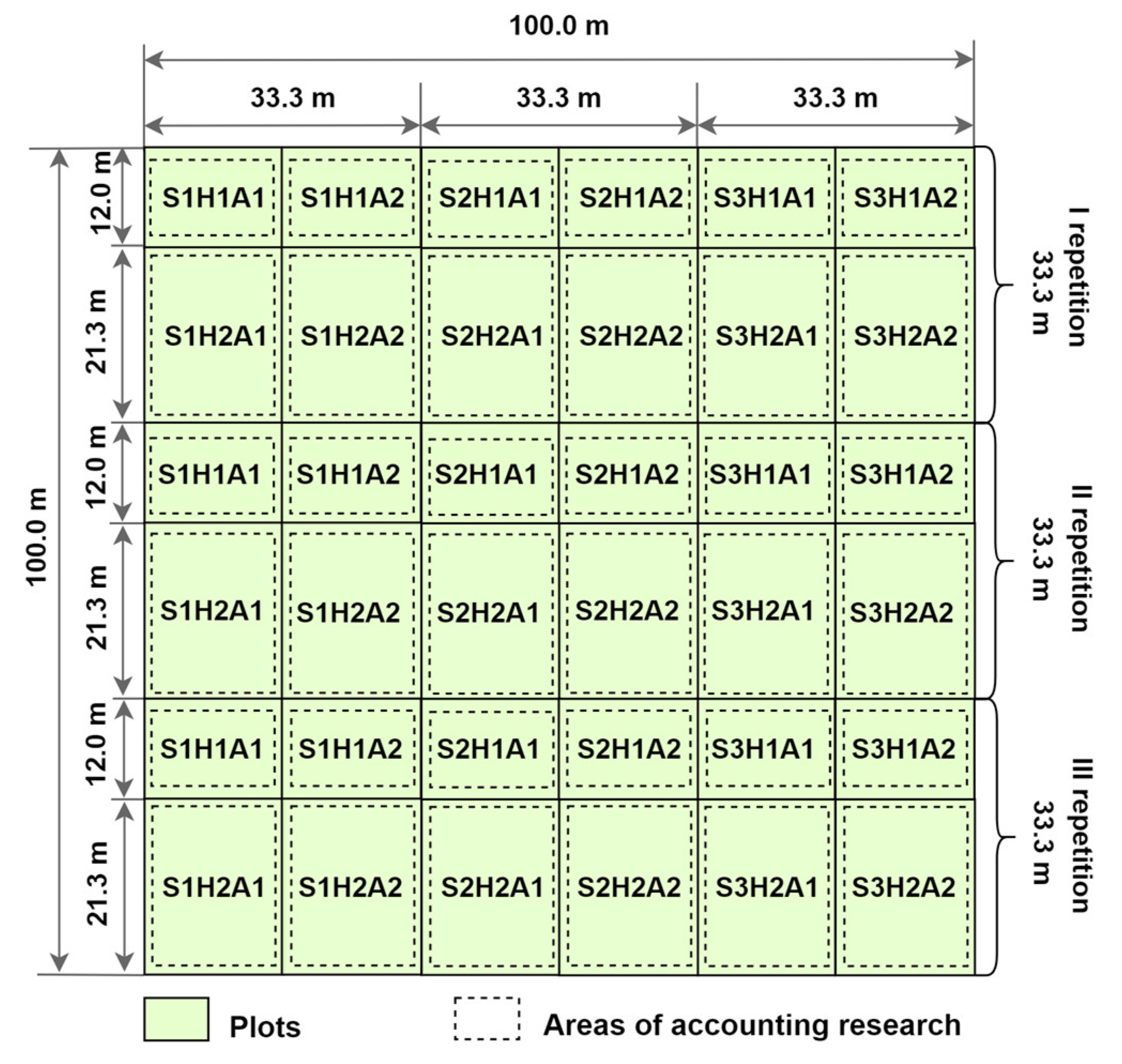
Figure 2.
The procedure for processing space images and images from drones. Flowering stage (shooting from a drone DJI Mavic 3M). A - image in pseudo-color; B - NDVI coefficient per pixel distribution; C - averaged values of the NDVI coefficient by fields.
Figure 2.
The procedure for processing space images and images from drones. Flowering stage (shooting from a drone DJI Mavic 3M). A - image in pseudo-color; B - NDVI coefficient per pixel distribution; C - averaged values of the NDVI coefficient by fields.
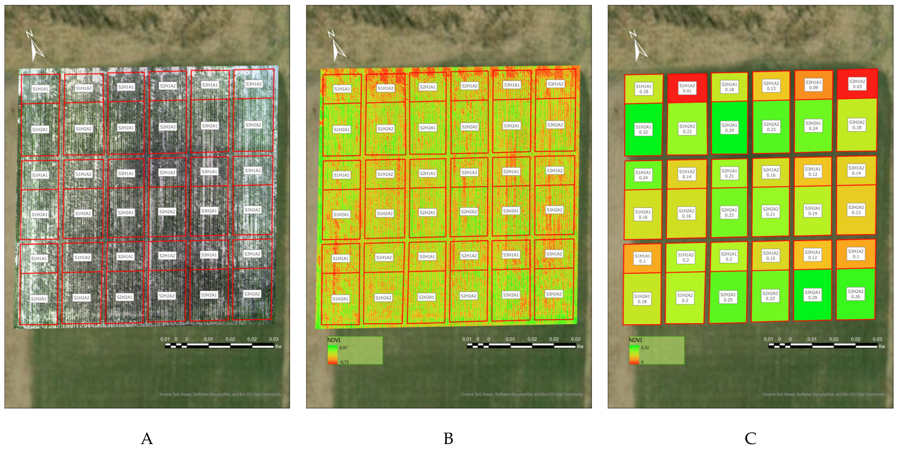

Table 1.
Database indicators.
| A group of indicators | Indicators |
|---|---|
| Type of processing | Tillage_sy, Herbicides, Sowing_den |
| Visual examination | Maize_height_cm, Maize_density_m2, Grass_weeds_number, Grass_weeds_density_m2, I_Dicotyledoneae_weeds_number, I_Dicotyledoneae_weeds_density_m2, II_Dicotyledoneae_weeds_number, II_Dicotyledoneae_weeds_density_m2, Root_weeds_number, Root_weeds_density_m2, Int_weed |
| Satellite data | VV, VH, B2, B3, B4, B8 |
| Drone data | G, R, RE, NIR, NDVI |
Table 2.
Variance analysis (ANOVA) for all channels of Sentinel-1, Sentinel-2 and drones for weed detection.
Table 2.
Variance analysis (ANOVA) for all channels of Sentinel-1, Sentinel-2 and drones for weed detection.
| Channel | Df | Sum | Sq Mean | Sq F | Value | Pr(>F) |
| VV | Tillage_system | 2 | 17.4 | 8.715 | 1.872 | 0.157 |
| Herbicides | 1 | 2.0 | 1.990 | 0.427 | 0.514 | |
| Sowing_density | 1 | 4.2 | 4.248 | 0.912 | 0.341 | |
| Residuals | 175 | 814.9 | 4.656 | |||
| VH | Tillage_system | 2 | 18.1 | 9.073 | 1.045 | 0.354 |
| Herbicides | 1 | 1.3 | 1.305 | 0.150 | 0.699 | |
| Sowing_density | 1 | 1.5 | 1.528 | 0.176 | 0.675 | |
| Residuals | 175 | 1519.7 | 8.684 | |||
| B2 | Tillage_system | 2 | 49854 | 24927 | 0.991 | 0.373 |
| Herbicides | 1 | 2102 | 2102 | 0.084 | 0.773 | |
| Sowing_density | 1 | 5571 | 5571 | 0.221 | 0.639 | |
| Residuals | 175 | 4403990 | 25166 | |||
| B3 | Tillage_system | 2 | 109883 | 54942 | 1.550 | 0.215 |
| Herbicides | 1 | 10554 | 10554 | 0.298 | 0.586 | |
| Sowing_density | 1 | 9437 | 9437 | 0.266 | 0.606 | |
| Residuals | 175 | 6201606 | 35438 | |||
| B4 | Tillage_system | 2 | 255469 | 127734 | 0.963 | 0.384 |
| Herbicides | 1 | 8563 | 8563 | 0.065 | 0.800 | |
| Sowing_density | 1 | 29341 | 29341 | 0.221 | 0.639 | |
| Residuals | 175 | 23207253 | 132613 | |||
| B8 | Tillage_system | 2 | 485977 | 242989 | 1.577 | 0.209 |
| Herbicides | 1 | 129754 | 129754 | 0.842 | 0.360 | |
| Sowing_density | 1 | 16495 | 16495 | 0.107 | 0.744 | |
| Residuals | 175 | 26958475 | 154048 | |||
| G | Tillage_system | 2 | 22183221 | 11091610 | 6.184 | 0.003 |
| Herbicides | 1 | 1141370 | 1141370 | 0.636 | 0.426 | |
| Sowing_density | 1 | 56954 | 56954 | 0.032 | 0.859 | |
| Residuals | 175 | 313870661 | 1793547 | |||
| R | Tillage_system | 2 | 13020158 | 6510079 | 2.849. | 0.061 |
| Herbicides | 1 | 18115158 | 18115158 | 7.927 | 0.005 | |
| Sowing_density | 1 | 1577901 | 1577901 | 0.690 | 0.407 | |
| Residuals | 175 | 399912227 | 2285213 | |||
| RE | Tillage_system | 2 | 1740347 | 870174 | 0.313 | 0.732 |
| Herbicides | 1 | 14970699 | 14970699 | 5.381 | 0.022 | |
| Sowing_density | 1 | 337323 | 337323 | 0.121 | 0.728 | |
| Residuals | 175 | 486873488 | 2782134 | |||
| NIR | Tillage_system | 2 | 15326079 | 7663039 | 11.86 | <0.001 |
| Herbicides | 1 | 18277361 | 18277361 | 28.29 | <0.001 | |
| Sowing_density | 1 | 6644403 | 6644403 | 10.29 | 0.002 | |
| Residuals | 175 | 113050243 | 646001 |
Df – degrees of freedom for each factor and residual values; Sum Sq – sums of each factor squares; Mean Sq – average squares; F value – the value of the F-statistic for each factor; Pr(>F) – p-value that allows to assess whether the effect of a factor is statistically significant.
Table 3.
Correlation analysis between the channels and the level of weediness.
| Channel | Weed correlations |
|---|---|
| VV | 0.1165 |
| VH | 0.1365 |
| B2 | -0.4276 |
| B3 | -0.3307 |
| B4 | -0.3584 |
| B8 | 0.3993 |
| G | -0.1821 |
| R | -0.2347 |
| RE | -0.2440 |
| NIR | 0.4007 |
Residuals:Min -416.48, 1Q -116.54, Median -13.84, 3Q 70.59, Max 886.84.
Table 4.
Regression analysis for Sentinel-1, Sentinel-2, and drone channels.
| Channel | Estimate Std. Error | t | value | Pr(>|t|) |
|---|---|---|---|---|
| (Intercept) | 4281.867 | 1229.373 | 3.483 | 0.001 |
| VV | 0.154 | 8.950 | 0.017 | 0.986 |
| VH | -18.581 | 7.300 | -2.545 | 0.012 |
| B2 | -9.145 | 1.070 | -8.549 | <0.001 |
| B3 | 8.481 | 1.449 | 5.853 | <0.001 |
| B4 | -0.977 | 0.648 | -1.509 | 0.133 |
| B8 | -0.358 | 0.108 | -3.326 | 0.001 |
| G | -0.033 | 0.047 | -0.687 | 0.493 |
| R | 0.020 | 0.044 | 0.451 | 0.652 |
| RE | 0.033 | 0.013 | 2.570 | 0.011 |
| NIR | 0.052 | 0.027 | 1.938 | 0.054 |
Residual standard error: 206.5 on 169 degrees of freedom. Multiple R-squared: 0.5406, Adjusted R-squared: 0.5134. F-statistic: 19.89 on 10 and 169 DF, p-value: < 0.001.
Table 5.
The Weed model.
| Residuals: |
Channel | Coefficients: | ||||
|---|---|---|---|---|---|---|
| Estimate Std. Error | t | value | Pr(>|t|) |
|||
| Call: lm(formula = weed_index ~ VV + VH, data = data) | ||||||
| Min | -313.04 | (Intercept) | 573.463 | 149.268 | 3.842 | <0.001 |
| 1Q | -171.20 | VV | 8.906 | 11.682 | 0.762 | 0.447 |
| Median | -81.68 | VH | 10.543 | 8.618 | 1.223 | 0.223 |
| 3Q | 51.15 | |||||
| Max | 1426.12 | Residual standard error: | 294.5 on 177 degrees of freedom | |||
| Multiple R-squared: | 0.022 | |||||
| Adjusted R-squared: | 0.011 | |||||
| F-statistic | 1.977 on 2 and 177 DF | |||||
| p-value | 0.142 | |||||
| Call: lm(formula = weed_index ~ B2 + B3 + B4 + B8, data = data) | ||||||
| Min | -353.10 | (Intercept) | 4144.249 | 1084.508 | 3.821 | <0.001 |
| 1Q | -132.90 | B2 | -7.851 | 0.828 | -9.485 | <0.001 |
| Median | -25.40 | B3 | 8.226 | 1.323 | 6.217 | <0.001 |
| 3Q | 103.00 | B4 | -1.365 | 0.597 | -2.288 | 0.023 |
| Max | 971.00 | B8 | -0.366 | 0.090 | -4.046 | <0.001 |
| Residual standard error: | 218.6 on 175 degrees of freedom | |||||
| Multiple R-squared: | 0.467 | |||||
| Adjusted R-squared: | 0.455 | |||||
| F-statistic | 38.370 on 4 and 175 DF | |||||
| p-value | <0.001 | |||||
| Call: lm(formula = weed_index ~ G + R + RE + NIR, data = data) | ||||||
| Min | -498.25 | (Intercept) |
-845.610 | 400.432 | -2.112 | 0.036 |
| 1Q | -144.68 | G | -0.050 | 0.057 | -0.874 | 0.383 |
| Median | -47.57 | R | 0.047 | 0.054 | 0.880 | 0.380 |
| 3Q | 61.73 | RE | -0.046 | 0. 013 | -3.705 | 0.000 |
| Max | 1319.33 | NIR | 0.152 | 0.030 | 5.046 | <0.001 |
| Residual standard error: | 261.2 on 175 degrees of freedom | |||||
| Multiple R-squared: | 0.239 | |||||
| Adjusted R-squared: | 0.222 | |||||
| F-statistic | 13.73 on 4 and 175 DF | |||||
| p-value | <0.001 | |||||
Table 6.
Model for assessing the weediness of maize crops with VV and VH channels of Sentinel-1 (Random Effect Model with Swamy-Arora’s transformation, one-way individual effect).
Table 6.
Model for assessing the weediness of maize crops with VV and VH channels of Sentinel-1 (Random Effect Model with Swamy-Arora’s transformation, one-way individual effect).
| Call: plm(formula = weed_index ~ VV + VH, data = pdata, model = “random”) | ||||||
| Effects: | Var | Std. dev | Share | |||
| idiosyncratic | 91096.6 | 301.8 | 1 | |||
| individual | 0.0 | 0.0 | 0 | |||
| theta: | 0 | |||||
| Residuals: | Channel | Coefficients: | ||||
| Estimate, S | Std. Error | z-value | Pr(>|z|) | |||
| Min | -313.04 | (Intercept) | 573.463 | 149.268 | 3.842 | 0.000 |
| 1Q | -171.20 | VV | 8.906 | 11.682 | 0.762 | 0.446 |
| Median | -81.68 | VH | 10.543 | 8.618 | 1.223 | 0.221 |
| 3Q | 51.15 | |||||
| Max | 1426.12 | Total Sum of Squares: | 15692000 | |||
| Residual Sum of Squares: | 15349000 | |||||
| R-Squared: | 0.022 | |||||
| Adj. R-Squared: | 0.011 | |||||
| Chisq | 3.953 on 2 DF | |||||
| p-value | 0.139 | |||||
Table 7.
Model for determining weed infestation in maize based on Sentinel-2 channel indicators (Random Effect Model with Swamy-Arora’s transformation, one-way individual effect).
Table 7.
Model for determining weed infestation in maize based on Sentinel-2 channel indicators (Random Effect Model with Swamy-Arora’s transformation, one-way individual effect).
| Call: plm(formula = weed_index ~ B2 + B3 + B4 + B8, data = pdata, model = “random”) | |||||||
| Effects: | Var | Std. dev | Share | ||||
| idiosyncratic | 43020.5 | 207.4 | 1 | ||||
| individual | 0.0 | 0.0 | 0 | ||||
| theta: | 0 | ||||||
| Residuals: | Channel | Coefficients: | |||||
| Estimate, S | Std. Error | z-value | Pr(>|z|) | ||||
| Min | -353.061 | (Intercept) | 4144.249 | 1084.508 | 3.8213 | 0.000 | |
| 1Q | -132.924 | B2 | -7.851 | 0.828 | -9.4850 | <0.001 | |
| Median | -25.397 | B3 | 8.226 | 1.323 | 6.2167 | <0.001 | |
| 3Q | 102.976 | B4 | -1.365 | 0.597 | -2.2881 | <0.001 | |
| Max | 970.953 | B8 | -0.366 | 0.090 | -4.0457 | <0.001 | |
| Total Sum of Squares: | 15692000 | ||||||
| Residual Sum of Squares: | 8359900 | ||||||
| R-Squared: | 0.467 | ||||||
| Adj. R-Squared: | 0.455 | ||||||
| Chisq | 153.486 on 4 DF | ||||||
| p-value | <0.001 | ||||||
Table 8.
Model to determine the weediness of maize crops with drone channel indicators (Random Effect Model with Swamy-Arora’s transformation, one-way individual effect).
Table 8.
Model to determine the weediness of maize crops with drone channel indicators (Random Effect Model with Swamy-Arora’s transformation, one-way individual effect).
| Call: plm(formula = weed_index ~ G + R + RE + NIR, data = pdata, model = “random”) | |||||||
| Effects: | Var | Std. dev | Share | ||||
| idiosyncratic | 61203.4 | 247.4 | 1 | ||||
| individual | 0.0 | 0.0 | 0 | ||||
| theta: | 0 | ||||||
| Residuals: | Channel | Coefficients: | |||||
| Estimate, S | Std. Error | z-value | Pr(>|z|) | ||||
| Min | -498.25 | (Intercept) | -845.611 | 400.432 | -2.112 | 0.0350 | |
| 1Q | -144.68 | G | -0.050 | 0.057 | -0.874 | 0.3820 | |
| Median | -47.57 | R | 0.047 | 0.054 | 60.880 | 0.3790 | |
| 3Q | 61.73 | RE | -0.046 | 0.013 | -3.705 | 0.0000 | |
| Max | 1319.33 | NIR | 0.152 | 0.030 | 5.047 | <0.001 | |
| Total Sum of Squares: | 15692000 | ||||||
| Residual Sum of Squares: | 11943000 | ||||||
| R-Squared: | 0.239 | ||||||
| Adj. R-Squared: | 0.222 | ||||||
| Chisq | 54.932 on 4 DF | ||||||
| p-value | <0.001 | ||||||
Disclaimer/Publisher’s Note: The statements, opinions and data contained in all publications are solely those of the individual author(s) and contributor(s) and not of MDPI and/or the editor(s). MDPI and/or the editor(s) disclaim responsibility for any injury to people or property resulting from any ideas, methods, instructions or products referred to in the content. |
© 2025 by the authors. Licensee MDPI, Basel, Switzerland. This article is an open access article distributed under the terms and conditions of the Creative Commons Attribution (CC BY) license (http://creativecommons.org/licenses/by/4.0/).
Copyright: This open access article is published under a Creative Commons CC BY 4.0 license, which permit the free download, distribution, and reuse, provided that the author and preprint are cited in any reuse.


