
Submitted:
27 May 2025
Posted:
28 May 2025
You are already at the latest version
Abstract
Although treeline ecotones are significant components of vulnerable mountain ecosystems and key indicators of climate change, treelines of the Southern Hemisphere remain largely out of research focus. In this study, we investigate, for the first time, the current and future distribution of the treeline species Nothofagus pumilio in the Southern Andes using a Species Distribution Modelling approach. The lack of modelling studies in this region can be contributed to missing occurrence data for the species. In a preliminary study, both point and raster data were generated using a novel Instagram ground truthing approach and remote sensing. Here we tested the performance of the two datasets: a typical binary species dataset consisting of occurrence points and pseudo-absence points and a continuous dataset where species occurrence was determined by supervised classification. We used a Random Forest (RF) classification and a RF regression approach. RF is applicable for both data sets, has a very good performance, handles multicollinearity and remains largely interpretable. We used bioclimatic variables from CHELSA as predictors. The two models differ in terms of variable importance and spatial prediction. While the RF classification model was mainly modelled by temperature variables, the RF regression model was mainly modelled by precipitation variables. Heat deficiency is the most important limiting factor for tree growth at treelines. It is evident, however, that water availability and drought stress will play an increasingly important role for the future competitiveness of treeline species and their distribution. Modelling with temperature variables in the RF classification model led to an overprediction of the potential distribution of the species in summit regions and in glacier areas, while the RF regression model led to a spatial prediction with small-scale details. The time-consuming and costly acquisition of complex species information should be accepted in order to provide better predictions and insights into the potential current and future distribution of a species.
Keywords:
climate change
; Nothofagus pumilio
; random forest algorithm
; species distribution modelling
; southern andes
; treelines
1. Introduction
The application of modelling approaches including Species Distribution Modelling (SDM) has rapidly increased recently in order to generate insights into the sensitivity and shifts of treelines in response to climate change [1]. Warming rates in high mountain regions are, on average, greater than the global mean, resulting in ecosystems being particularly stressed by changing climatic conditions [2]. The natural elevational position of the treeline is defined by heat deficiency [3] and is globally approximately aligned with the 6.4 °C isotherm [4]. Consequently, treeline shift in response to warming is frequently investigated and widely recognised as a key indicator of climate change [5]. However, observed responses are rather inconsistent, spanning the entire gradient from static treelines with insignificant responses to dynamic treelines with substantial treeline advance [6,7]. Globally, the proportion of advancing elevational treelines has been increasing from 52 % [8] to 66 % [9,10]. In the Northern Hemisphere, 90 % of treelines are reported to be advancing [11], whereas treelines in the Southern Hemisphere are responding weaker to climatic changes [10]. Certain relationships between treeline form, which can vary between gradual and abrupt, and treeline dynamics have been suggested [12]. Factors such as seedling mortality and dieback processes play critical roles in shaping treeline form and influencing possible shifts [13]. While gradual treelines are more likely to advance to higher elevations, abrupt treelines, as formed by Nothofagus in the Southern Hemisphere, are more stable due to increased seedling mortality above closed forest stands or due to anthropogenic disturbances [13].
Treelines and the shift of treelines have extensively been studied in the last decades [1,14], however, comparatively few studies focused on treelines of the Southern Hemisphere [9,10]. A recent review study examining the impact of climate change on Andean biomes found that those in the southern Andes remain the least studied [15]. For example, to our knowledge, there is no SDM study investigating the entire current and future distribution of important treeline species in the Southern Andes. Nothofagus pumilio (Poepp et Endl.) Krasser (southern or lenga beech) is forming an abrupt treeline over approximately 2000 km latitudinal extent from 35 °S to 56 °S in the Southern Andes. The treeline is naturally abrupt due to seedling dieback outside the protecting tree stands [16], only in some cases the treeline is influenced by anthropogenic disturbances like grazing, forestry or fire resulting in more diffuse treeline ecotones [13]. The uppermost trees are often in a krummholz growth form [17]. The treeline follows a 6.6 °C isotherm [18], while increases of 1.2 to 4.0 °C in mean annual temperatures and decreases of up to 30 % in mean annual precipitation are predicted for high-elevation catchments in the southern Andes [19,20]. It is therefore of interest to study the changes in the Southern Andean treeline as a result of global warming.
Recent research has explored changes at the treeline of N. pumilio through small-scale dendrochronological and experimental studies [21,22,23,24,25]. N. pumilio is highly sensitive to variations in temperature and precipitation, which are often associated with phase shifts in Antarctic Decadal Oscillation (AAO) also known as the Southern Annular Mode (SAM), the El Niño Southern Oscillation (ENSO) and Pacific Decadal Oscillation (PDO), as highlighted in recent studies [21,22,23]. Increases in radial growth due to rising temperatures have been observed when precipitation levels are sufficient [21,24,25]. Warm and dry springs lead to an increased tree growth at humid treeline sites but to a decrease in tree growth and an increase of tree mortality due to drought at drier treeline sides. Furthermore, high precipitation in late spring often connected with a prolonged snow cover results in a decrease in tree growth [21]. Accordingly, tree growth is highest at mesic sites, followed by wetter sites, while growth rates at drier sites continue to decline [24]. Suitable climatic conditions, particularly rising mean spring and summer temperatures, also promote the establishment of N. pumilio seedlings above the current treeline, on both humid and dry slopes, thereby facilitating treeline advance [22,23]. Additionally, warmer springs can improve seed quantity and quality [26] which further increases the possibility of seedlings becoming established. However, drought or soils with low water capacity are important controlling factors, causing drought stress for seedlings and adult trees [27] and ultimately preventing a treeline advance.
In this study, we model the potential current and future distribution of N. pumilio based on the species’ suitable bioclimatic conditions, following fundamental concepts of Species Distribution Modelling (SDM). SDM models are typically constructed using binary species occurrence data and environmental variables, often climate data [28]. While global climate data sets, such as the CHELSA bioclimatic variables that we use here [29,30], are readily available, the availability of unbiased species occurrence data is a major challenge for SDM studies. Field studies, which can generate reliable occurrence data, are both time-consuming and costly. Moreover, many study sites, particularly in topographic complex regions like high mountains are inaccessible. When species data are not collected through field studies, they are primarily obtained from open-source databases such as the Global Biodiversity Information Facility (GBIF, https://www.gbif.org/). However, these databases often contain various forms of bias, as highlighted in recent studies [31,32]. Consequently, using these point occurrences in SDM approaches can lead to inaccurate or misleading model results. A promising approach for the investigation of large study areas, especially in regions with limited accessibility, is the use of remote sensing to survey species occurrences. Remote sensing data on a species can provide more complex, continuous data and thus further modelling opportunities. However, there is still a need for ground truthing to verify that the species of interest are actually present in the remotely sensed area. In a previous study we developed an Instagram ground truthing approach, that created less-biased occurrence points, that were subsequently used to validate remote sensing occurrence data of N. pumilio, resulting in two valid occurrence datasets [33].
Here, we present an initial holistic approach to model the potential distribution of N. pumilio based on two input datasets: a binary point dataset and a continuous raster occurrence dataset derived from supervised classification. While we adopted a standard modelling approach, we also test an innovative technique incorporating continuous raster data. We hypothesise that this approach will yield more detailed insights into the species' potential current and future distribution due to the increased complexity of input data.
To investigate the effect of different species input datasets, our aims are (1) to model the current distribution of N. pumilio under prevailing climate conditions, and (2) assess potential range shifts under climate change conditions, and (3) evaluate model performance and model complexity with regard to ecological site factors.
2. Materials and Methods
2.1. Study Species and Study Area
N. pumilio is the most orophilous and widespread species of the Nothofagus genus on the South American continent, extending from 35 °S to the southernmost tip of Tierra del Fuego (see Figure 1). As an indicator of the orotemperate belt, it forms mono-species forests at the treeline [34]. The species is sometimes accompanied by the morphologically and ecologically similar species N. antarctica, with which it can form mixed stands. Hybrids between the two species are also known [35]. The evergreen N. betuloides dominates in the lowlands and especially in the (hyper-) humid west.
The study area is characterised by two extreme gradients. One is the temperature gradient, which results from the elevation of the southern Andean Cordillera (up to 3000 m), and the other is the precipitation gradient, which is considered to be the most extreme precipitation gradient on Earth. While precipitation extremes of up to 10,000 mm/yr occur on the windward side, west of the Andes, there is a precipitation decrease to less than 300 mm/yr on the leeward side, east of the Andes [36]. Northern Patagonia has been substantially affected by the effects of climate change. Mean annual temperatures have risen by up to 1 °C since 1950. While there are no negative trends in precipitation in most areas, precipitation totals are decreasing by 5 % in Northern Patagonia. Climate models predict a decrease in precipitation of up to 30 % and an increase in temperature of between 1.5 and 3 °C [20].
2.2. Input Data
2.2.1. Species Data
The two species occurrence datasets used were generated using a novel Instagram ground truthing approach (IGTA) designed to reduce sampling and spatial bias often present in existing databases. The IGTA aimed at reducing this bias by using a very public and worldwide used social media platform (https://www.instagram.com/) and by including remote sensing data [33]. The study species and area are particularly well-suited for an Instagram-based analysis, as deciduous N. pumilio forms mono-species forests at the treeline, making it an especially attractive photo motif in autumn and occurs in a highly touristic region, where tourists and hikers frequently take and share photos on social media. By searching for suitable posts with the species and the photos’ location clearly identifiable as well as a strict catalogue of criteria 1238 occurrence points were created extending from 36.88 °S to 55.03 °S. These IGTA points were then used to validate remote sensing data created using Sentinel-2 level 2A data and supervised classification [33]. With this approach two data sets were created: A point occurrence dataset and a spatial raster dataset of the species N. pumilio (Figure 1).
For the IGTA point dataset the first step in modelling was to ensure that only one point was set in a raster cell at the target resolution of 30 arc sec, ~ 1 km (raster cell size of the climate data). After deleting duplicate points, 999 points remained in the model as “presence” data. For “absence” data, 10,000 pseudo-absence points were generated. This process involved first constructing an alpha hull around the presence points and applying a 100 km buffer, within which pseudo-absence points were randomly generated. To prevent the overwriting of occurrence cells during this process, a 5 km buffer was placed around the presence points. For the final modelling dataset, values from the climate dataset were extracted for both presence and absence points. The two datasets were then merged and supplemented with a binary indicator variable specifying whether N. pumilio was present (presence = 1) or absent (absence = 0).
The second dataset was derived from a supervised classification (Kappa values: summer scenes classification 0.89, autumn scenes classification 0.96), in which occurrences of deciduous forest at the treeline were classified to represent the distribution of N. pumilio [33]. Gaps in the dataset resulted from missing Sentinel-2 data or areas affected by shadows and cloud cover. The original dataset has a spatial resolution of 20 m. For modelling purposes, N. pumilio cover values were aggregated to the target resolution (~1 km), resulting in percentage values ranging from close to 0 % up to a maximum of 99.96 %. The raster data covers a latitudinal range from 33.49 °S to 56.27 °S.
2.2.2. Bioclimatic Predictors
Global climatological datasets such as CHELSA [29,30] and Worldclim [37,38] are standards for large-scale SDM studies. Due to their free accessibility, the datasets are widely used and cited, allowing for some comparability of modelling studies. Since other studies suggest that the CHELSA dataset performs better in topographically highly complex areas such as high mountains [39,40], we decided to use this dataset. We utilised the 19 Bioclim variables from version 2.1 with a 30 arc sec (~1 km) resolution [29,30]. The “ClimDatDownloadR” R package was used to download and pre-process the data [41,42]. To enhance ecological interpretability, we included only variables derived for quarters. To further mitigate multicollinearity and exclude irrelevant variables, we applied the VSURF R package, which follows a two-step procedure. First, it identifies variables relevant for interpretation, and subsequently, it eliminates redundant variables for prediction [43]. Through this approach, two additional variables were removed from the initial subset. The variables used in the model are listed and described in Table 1.
For future prediction CHELSA version 2.1 provides selected CMIP6 scenarios of the bioclimatic variables. Future Bioclim variables were created using representative concentration pathway (RCP) scenarios, that represent a range of potential greenhouse gas emission pathways, from a low-emission (RCP2.6) to a high-emission development (RCP8.5). We used the SSP126 (RCP2.6), SSP370 (RCP7) and SSP585 (RCP8.5) scenarios for the years 2041 to 2070 and 2071 to 2100 from the MPIESM1-2HR model [30].
2.3. Model Approach and Model Algorithm
We follow the basic concepts of Species Distribution Modelling (SDM) to analyse the relationship between the species' current distribution and suitable abiotic conditions, as well as its potential future distribution under climate change scenarios [44,45].
Several algorithms have been established for SDMs. In addition to linear regression approaches such as Generalised Linear Models (GLMs), Generalised Additive Models (GAMs) and Multivariate Adaptive Regression Splines (MARS), machine learning algorithms such as Random Forest (RF), Maximum Entropy (MaxEnt) and Artificial Neural Networks (ANN) are established methods [46]. We chose RF because it can be used for classifying binary data (Random Forest Classification), as well as for regression approaches with continuous data (Random Forest Regression) [47]. Furthermore, machine learning approaches such as RF not only demonstrate strong predictive power and model performance but are also unaffected by multicollinearity, making them particularly well-suited for climatic datasets with many highly correlated variables [48]. However, some authors criticise that the interpretability of the models decreases as machine learning methods are “black boxes” compared to simpler linear approaches (e.g. GLMs) [46,48,49]. Random Forest combines both strengths: it is a robust and powerful approach that remains largely interpretable. In the following we analysed two models: (1) RF classification with the point dataset and (2) RF Regression with continuous data from the raster dataset. We apply a k-fold cross-validation to determine the best model and use appropriate validation metrics for each model. The results of the models are then compared visually.
Data processing and modelling were conducted in R (version 4.4.1 [50]). Maps were created using SAGA GIS (https://saga-gis.sourceforge.io [51]) and ArcGIS Pro (version 2.7.0 [52]).
2.4. Model Calibration and Evalution
We used 10-fold cross-validation to determine the best model. The presence-absence point dataset, and the continuous raster dataset were randomly divided into a training and a test dataset. The training dataset contains 80 % and the test dataset 20 % of the total dataset. Several validation metrics were used to validate the models. Threshold-independent metrics such as AUC and threshold-dependent metrics such as TSS are appropriate for the presence-absence approach. Furthermore, we created confusion matrices and calculated overall accuracy. The explained variance, the mean of the squared residuals and the R2 are suitable for validating the RF regression for the continuous approach. 100 trees were calculated for both, RF classification and RF regression. The best model was then projected onto the CHELSA data calculated with the CMIP6 scenarios (SSP126, 370, 585 for the time spans of 2041 – 2070 and 2071 – 2100).
3. Results
3.1. Current Distribution Range of N. pumilio
The optimal model for predicting the current distribution of N. pumilio was identified through 10-fold cross-validation. The results of the cross-validation for both models are presented in Table 3 and Table 4 in the appendix section. The best-performing RF classification model achieved an accuracy of 97.74 %, with a threshold-independent AUC of 0.9919 and a threshold-dependent TSS of 0.8467. Bioclimatic variables bio 8 (mean daily mean air temperature of the driest quarter) and bio 11 (mean daily mean air temperature of the coldest quarter) emerged as the most influential predictors for model accuracy (Accuracy Importance ranking, from most to least important bioclimatic variable: 8, 11, 19, 4, 15, 10, 18, 17, cf. Table 1). Additionally, Gini Importance was calculated to assess the most frequently used variables for decision at nodes, with bio 11 and bio 8 again emerging as the primary split criteria for the RF classification model (Gini Importance ranking: 11, 8, 18, 17, 19, 4, 10, 15). The highest-performing RF regression model attained an R2 value of 0.6680 and the lowest RMSE of 140.92. While temperature variables were the most important predictors in the RF classification model, precipitation-related variables, particularly bio 15 (precipitation seasonality) and bio 19 (mean monthly precipitation amount of the coldest quarter), played a dominant role in the RF regression model (Accuracy Importance ranking: 15, 19, 4, 11, 18, 8, 17, 10). Gini Importance analysis for the RF regression model indicated that bio 11 was the most critical variable for splits, followed by bio 15 (Gini Importance ranking: 11, 15, 18, 8, 17, 4, 10, 19).
A RF model consists of multiple individual decision trees, making it challenging to interpret the specific thresholds used at each node. However, the extraction of partial dependence plots (PDP) for individual variables allows for an interpretation of the influence of specific bioclimatic predictors within the RF model. We employed the “partialPlot” function from the “randomForest” (version 4.7-1.2 (2024), [53]) R package to assess the influence of the most important variable in each model. The resulting PDP are presented in Figure 2. For the RF classification model, the x-axis displays the values of the bioclimatic variable bio 8, while the y-axis represents the predicted probability for class 1 (i.e., presence of N. pumilio). At low temperatures in the wettest quarter (below - 5 °C), the predicted probability of occurrence is high, clearly decreasing towards 5 °C and remaining consistently low above this threshold. This indicates that the model predicts the presence of N. pumilio primarily in colder environments during the wettest quarter. In the RF regression model, the x-axis shows the values of bio 15, and the y-axis represents the predicted cover values of N. pumilio. The plot reveals greater variability, but cover values are relatively high in areas with moderate precipitation seasonality (0 to 30 %). However, there is a marked decline in predicted cover values in regions with high precipitation seasonality (70 to 100 %). Two key assumptions emerge: cover values are greater in areas with lower precipitation seasonality, suggesting that N. pumilio prefers regions with more stable precipitation patterns and the species is less likely to occur in areas with highly variable precipitation e.g. with phases of drought.
The spatial predictions of the two models revealed a more compact distribution in the RF classification model, with a slightly broader extent towards the west and east for the RF regression model. The binary RF classification model predicted a northern extent of up to 36.35 °S and a southern extent of 55.45 °S, whereas the RF regression model extended from 35.24 °S to 55.24 °S (Figure 3). In the southern regions, including Tierra del Fuego, the RF regression model depicted a more homogeneous distribution. IGTA points were lacking in this area resulting in gaps in the predicted occurrence. While the RF classification model tended to overpredict in unvegetated summit regions and glaciated areas, the RF regression model provided a more fine-grained representation, capturing vegetated valleys more accurately. When compared with a digital surface model (DSM, ALOS Global Digital Surface Model, 30 m), it was evident that the RF classification model predicted suitable climatic conditions in higher areas as distribution areas, while in the RF regression model they were omitted. The opposite was true for lower valleys. Here, the RF regression model predicted suitable climatic conditions of N. pumilio, while the RF classification model did not. The described small-scale differences between the models are illustrated in Figure 4.
3.2. Future Distribution Range of N. pumilio
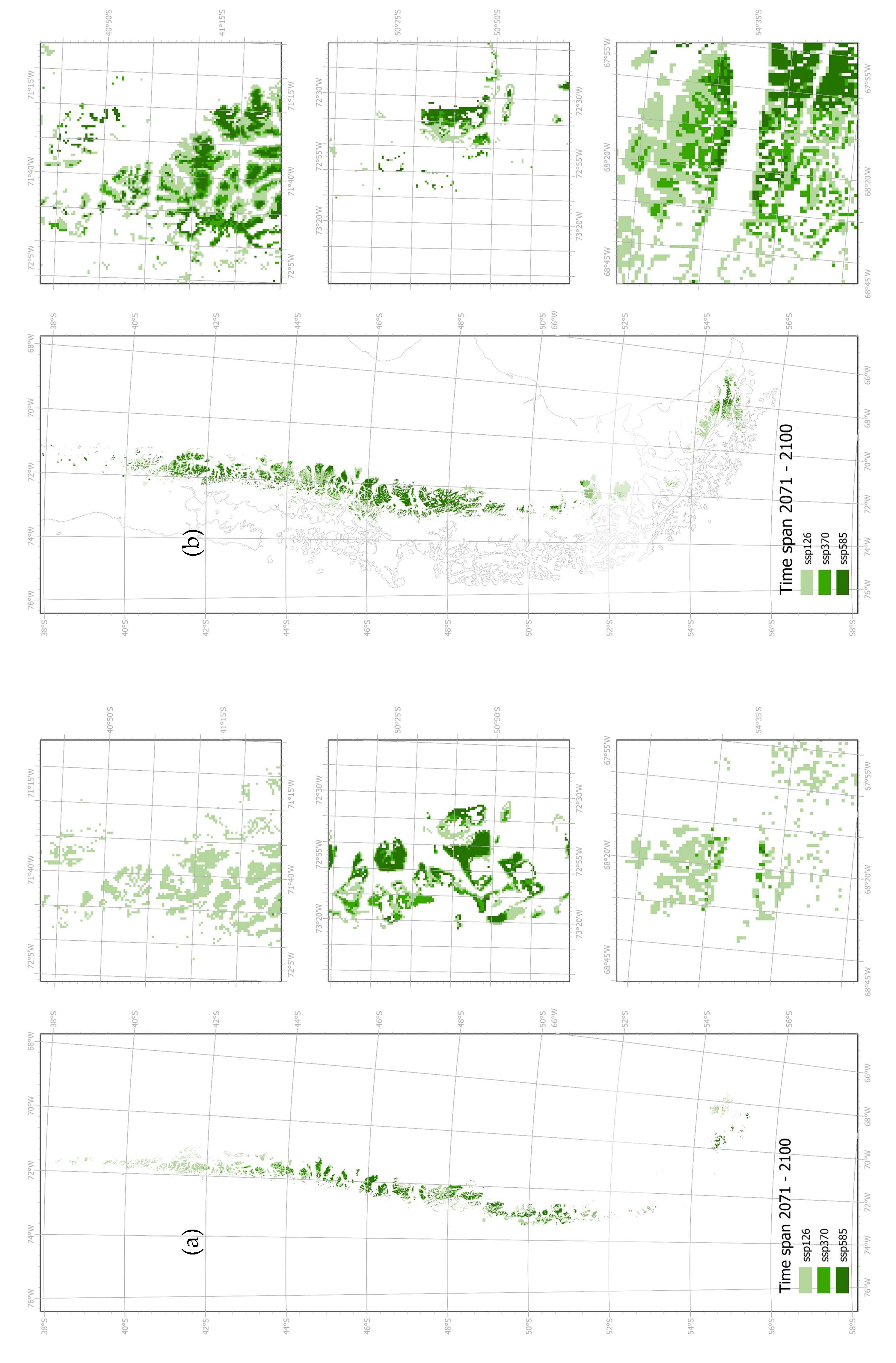
Using CMIP6 data provided by CHELSA for the SSP scenarios, we predicted the potential future distribution of N. pumilio with both models. Predictions were generated for the SSP126, SSP370, and SSP585 scenarios for two future periods: 2041–2070 and 2071–2100. Figure 5a,b illustrate the potential distribution of N. pumilio for 2041–2070, while Figure 6a,b in the appendix depict projections for 2071–2100. To further quantify these changes, we calculated the total area covered by N. pumilio pixels in each model. A direct comparison of absolute values was not feasible, as different thresholds were applied in the binary representation of the models, which could distort the results. However, we calculated the future projected area as a percentage of the current distribution area, allowing for a meaningful comparison of relative changes (Table 2). For the RF classification model, the SSP scenarios for 2041–2070 indicated a progressive decline in occurrences across the northern range. Additionally, occurrences shifted towards higher elevations and the more humid western regions, while a slight decline was also observed in the south. These trends intensified from 2071 to 2100, with a further reduction in western occurrences. The overall contraction in N. pumilio distribution was reflected in the decreasing area of grid cells that are covered by a models result. The current distribution area of N. pumilio calculated by the RF classification model is 39,732.83 km². Even under the relatively mild SSP126 scenario, only 37.54 % of this area (14,916.48 km², see Table 2) remained, with further declines projected for more extreme scenarios and later time periods. A slight increase in area was observed for SSP585 during 2041–2070, which can be attributed to an expansion in the west. The RF regression model predicted less pronounced changes in N. pumilio cover values, which might have been partially due to the use of a threshold for generating a binary representation. Unlike the RF classification model, which assigned values of 1 (presence) or 0 (absence), the RF regression model predicted a continuous coverage percentage. For visualisation and quantitative analysis, a threshold of 30% was applied, classifying all values above 30 % as presence (1) and all values below 30 % as absence (0). Both models indicated a decline in occurrences in the north. However, in contrast to the RF classification model, the RF regression model suggested that N. pumilio is more likely to persist at higher elevations also in the north. Total decreases in distribution area and the westward shift were less pronounced, and occurrences in the east were more likely to remain. Overall, an upward shift in elevation was evident across the species' range.
4. Discussion
The treeline species Nothofagus pumilio is highly sensitive to climate variations, as reflected in its radial growth patterns and seedling establishment above the treeline. Consequently, research into the species' treeline dynamics in response to climate change has already gained some attention. Many studies have examined growth variations using dendrochronology, providing insights into the species' response to climate variations, mostly related to expressions in ENSO, PDO and AAO/SAM over the past century [21,24,25]. Other research has focused on seedling establishment [23] or assessed the quantity and quality of N. pumilio seeds [16,54,55]. However, large-scale Species Distribution Modelling (SDM) approaches investigating the current and future development of the species are lacking. In this study, we calculated two Random Forest (RF) models using a binary and a continuous species dataset to model the current and future potential distribution of the species. Both models, RF classification and RF regression, achieved reasonable results and high performance values. The RF algorithm is well-suited for this study due to its strong predictive power and, more importantly, its applicability to both datasets, enabling direct comparability. Moreover, RF is a well-established algorithm that facilitates comparisons between different modelling approaches within the field of SDM [46,56]. While binary approaches are mainly used in SDM, the use of a continuous target variable generated from remote sensing, rather than the generation of abiotic predictors, is still a novel approach. Other studies investigating topographic complex regions have already discussed the loss of knowledge due to the use of binary data at 1 km spatial resolution [49]. Here, we demonstrated an information gain using 1 km-resolution data while incorporating continuous variables.
4.1. Current Distribution Range of N. pumilio
Differences between the two models were apparent across all analyses. In terms of spatial prediction, the RF regression model captured fine-scale details more accurately and was less prone to overprediction at high elevations. Additionally, the key predictors for the RF models varied. While temperature variables had the highest importance (Accuracy Importance) in the RF classification model, precipitation variables had the highest importance in the RF regression model. The orophilous species N. pumilio is particularly adapted to the extreme climatic conditions of high mountain ecosystems. The species shows high phenotypic plasticity. While occurring at lower elevations as an erect tree up to a height of 35 m, it shows krummholz growth forms at the treeline [57]. As a deciduous species, it reduces transpiration in the months when frost-drought can be a problem [58]. Heat deficiency is considered to be the most important site factor for treeline formation worldwide. The treeline of N. pumilio follows an isotherm of 6.6 °C [18]. The influence of temperature was shown in the RF classification model by the high importance of bio 8 (mean daily air temperature of the driest quarter) and bio 11 (mean daily air temperature of the coldest quarter), and in both models by the fact that the variable bio 11 has a very important influence on the decisions at the nodes of both models (Gini Importance). However, when modelling a species in high mountains, the influence of elevation can also be represented by temperature variables. Authors analysing the sensitivity of N. pumilio to climate change using changes in tree rings have found a correlation with precipitation regimes in addition to temperatures. The species occurs in humid to arid regions and is well adapted to medium to low precipitation sums that occur at high elevations due to advective precipitation. This is also shown by its occurrence as far as the arid east, where it sometimes forms two treelines: an alpine treeline and a xeric treeline towards the arid steppes [59]. However, particularly in northern Patagonia, increasingly low precipitation during the spring and summer months negatively affects tree growth [21,60]. In more southerly regions, high spring precipitation is primarily associated with prolonged snow cover, leading to a shortened growing season, which in turn also hinders tree growth [21,61,62]. Between 1900 and 2020, tree growth was found to correlate most strongly with rising temperatures on mesic sites, followed by wetter sites, while growth rates declined on drier sites [24]. Some authors state that all treelines in southern South America have experienced a negative growth trend due to drought since the 1980s and even suggest that the limitation at the treeline has changed from cold-limited to drought-limited [25,63]. Our results of the RF regression model seem more plausible in this context, as the precipitation variables bio 15 (precipitation seasonality) and bio 19 (mean monthly precipitation of the coldest quarter) played an important role. Both variables reflect annual precipitation distribution patterns. Bio 15 suggests that N. pumilio is unlikely to occur in regions with high precipitation seasonality, which may be associated with periods of drought. Bio 19, on the other hand, may be linked to precipitation in the form of snow, the resulting snow cover, and water availability following thaw.
4.2. Future Distribution Range of N. pumilio
Abrupt treelines respond less to global warming than diffuse treelines, primarily due to higher seedling mortality outside the protecting forest stand climate [13]. The emergence and establishment of seedlings represent the most critical life stage for trees at the treeline, with the availability of species-specific safe sites being the basic precondition for seedling recruitment [64,65]. Seed production, fruit dispersal, seed viability, and seedling establishment all decline with increasing elevation [16]. Higher temperatures and an extension of the growing season can thus facilitate seedling emergence and survival [18,22,23,54,60], a precondition for a future treeline advance. However, the comparatively slow advance or persistence of the treeline in the southern Andes is also linked to multi-faceted interactions with edaphic, topographic, biotic and other factors, including the development of alpine mats [23,27]. In addition, a deterioration in growth conditions due to drought is predicted for occurrences at lower elevations as well as at the treeline, based on studies examining radial tree growth [25,63]. The use of CMIP6 SSP scenarios from CHELSA showed an advance to higher elevations in both models. The scenarios are based on global circulation models and CO2 concentration estimates. It should be noted that less periodic variations caused by different phases of ENSO, PDO and AAO/SAM cannot be fully modelled in the scenarios [66]. While the RF classification model showed a significant decrease in the northern range, lower cover values of the RF regression model remained at higher elevations. The result that N. pumilio occurrences decreased at lower elevations is consistent with previous findings [54], highlighting a decrease in the number of seedlings and a reduction in survival at lower-elevated sites. A review study modelling biome-level changes predicts a reduction of area with suitable climatic conditions for temperate deciduous forests of approximately 30 % under the RCP8.5 scenario for the period 2040–2070 [15]. Our results from the RF regression model are congruent with these findings, whereas the RF classification model predicts an even greater decline, which can be attributed to overprediction at high elevations. In particular, the RF classification model predicted a shift towards the wetter western region. It will be necessary to investigate the future competitive relationships with dominant tree species in this area (e.g. N. betuloides). In summary, precipitation conditions/drought stress will play a significant role in future competitive relationships and successful regeneration of Nothofagus species in the southern Andes.
5. Conclusions
To our knowledge, this is the first SDM study that models the current and future distribution of N. pumilio across its entire distribution range in the southern Andes. Even though the distribution range encompasses two extreme climatic gradients both models were able to comprehensively predict the current potential distribution and its future development. The direct comparison of model approaches highlighted major differences of the model results and the advantages of using more complex, continuous data. Continuous data can provide better insights into suitable bioclimatic conditions for N. pumilio occurrence leading to more detailed spatial predictions and meaningful predictors based on variable importance. However, we acknowledge that such data are rarely available, difficult to obtain across large study areas, and may still contain gaps that introduce bias. Climatic parameters represent the principal limiting factors at the alpine treeline, and bioclimatic variables have already proven effective in capturing the climatic conditions at the treeline of the southern Andes. In the future we will embed biotic variables and try to model other influences such as fire, grazing and forestry.
Author Contributions
Conceptualization, M.W., J.B., J.O., U.S., J.W., M.B..; methodology, M.W, J.O., J.W., M.B.; validation, M.W., J.O., M.B.; formal analysis, M.W.; investigation, M.W.; data curation, M.W.; writing—original draft preparation, M.W.; writing—review and editing, M.W., J.B., J.O., U.S., M.B.; visualization, M.W.; supervision, J.B. and U.S. All authors have read and agreed to the published version of the manuscript.
Funding
This research received no external funding.
Data Availability Statement
The species input data used in this study are online available at the free data provider of University of Hamburg: http://doi.org/10.25592/uhhfdm.16239
Conflicts of Interest
The authors declare no conflicts of interest.
Appendix A
Appendix A.1
Figure 6.
Potential future distribution of Nothofagus pumilio modelled by (a) the Random Forest classification and (b) RF regression model using CMIP6 SSP Scenarios for CHELSA Bioclim variables for the time span of 2071 to 2100.
Figure 6.
Potential future distribution of Nothofagus pumilio modelled by (a) the Random Forest classification and (b) RF regression model using CMIP6 SSP Scenarios for CHELSA Bioclim variables for the time span of 2071 to 2100.
Appendix A.2

Table 3.
Individual binary point model 10-fold cross-validation performance results. The best model (model no. 4) is highlighted in bold caps. The numbers for the confusion matrix (cfm) are: 00 true negative, 01 false positive, 10 false negative and 11 true positive.
Table 3.
Individual binary point model 10-fold cross-validation performance results. The best model (model no. 4) is highlighted in bold caps. The numbers for the confusion matrix (cfm) are: 00 true negative, 01 false positive, 10 false negative and 11 true positive.
| No | set.seed | cfm (train) (00, 01, 10, 11) | cfm (test) (00, 01, 10, 11) | Accuracy (test) [%] | AUC | TSS (test, without threshold) |
|---|---|---|---|---|---|---|
| 1 | 123 | 7774, 105, 152, 645 | 1936, 36, 31, 166 | 0.9691 | 0.9866 | 0.8060 |
| 2 | 321 | 7736, 106, 154, 680 | 1977, 29, 27, 136 | 0.9742 | 0.9928 | 0.8108 |
| 3 | 456 | 7762, 115, 154, 645 | 1946, 30, 23, 170 | 0.9756 | 0.9922 | 0.8383 |
| 4 | 654 | 7736, 118, 158, 664 | 1968, 25, 24, 152 | 0.9774 | 0.9919 | 0.8467 |
| 5 | 789 | 7790, 104, 159, 623 | 1926, 38, 26, 179 | 0.9705 | 0.9929 | 0.8116 |
| 6 | 987 | 7768, 112, 157, 639 | 1939, 39, 27, 164 | 0.9696 | 0.9900 | 0.7941 |
| 7 | 111 | 7774, 105, 151, 646 | 1945, 42, 22, 160 | 0.9705 | 0.9894 | 0.7809 |
| 8 | 222 | 7757, 110, 163, 646 | 1954, 38, 25, 152 | 0.9710 | 0.9868 | 0.7874 |
| 9 | 333 | 7755, 103, 143, 675 | 1958, 33, 30, 148 | 0.9710 | 0.9886 | 0.8026 |
| 10 | 444 | 7731, 122, 154, 669 | 1969, 36, 24, 140 | 0.9723 | 0.9890 | 0.7834 |
Table 4.
Individual raster model 10-fold cross-validation performance results. The best model (model no. 8) is highlighted in bold caps.
Table 4.
Individual raster model 10-fold cross-validation performance results. The best model (model no. 8) is highlighted in bold caps.
| No. | set.seed | explained var. (train) | RMSE1 (train) | RMSE1 (test) | R2 (test) |
|---|---|---|---|---|---|
| 1 | 123 | 65.44 | 147.24 | 141.76 | 0.661 |
| 2 | 321 | 65.53 | 146.12 | 146.27 | 0.657 |
| 3 | 456 | 65.38 | 147.02 | 141.42 | 0.666 |
| 4 | 654 | 65.51 | 146.32 | 145.14 | 0.659 |
| 5 | 789 | 65.43 | 146.34 | 146.30 | 0.659 |
| 6 | 987 | 65.57 | 145.74 | 145.31 | 0.661 |
| 7 | 111 | 65.52 | 146.38 | 142.82 | 0.663 |
| 8 | 222 | 65.29 | 147.30 | 140.92 | 0.668 |
| 9 | 333 | 65.48 | 146.72 | 143.09 | 0.661 |
| 10 | 444 | 65.47 | 146.46 | 142.80 | 0.664 |
1 Root mean square error
References
- Holtmeier, F.-K.; Broll, G. Treeline Research—From the Roots of the Past to Present Time. A Review. Forests 2020, 11, 38. [Google Scholar] [CrossRef]
- Schickhoff, U.; Bobrowski, M.; Mal, S.; Schwab, N.; Singh, R.B. The World’s Mountains in the Anthropocene. In Mountain Landscapes in Transition; Schickhoff, U., Singh, R.B., Mal, S., Eds.; Springer International Publishing: Cham, 2022; pp. 1–144. ISBN 978-3-030-70237-3. [Google Scholar]
- Körner, C. Climatic Controls of the Global High Elevation Treelines. In Encyclopedia of the World's Biomes; Elsevier, 2020; pp. 275–281. ISBN 9780128160978. [Google Scholar]
- Paulsen, J.; Körner, C. A climate-based model to predict potential treeline position around the globe. Alp Botany 2014, 124, 1–12. [Google Scholar] [CrossRef]
- Qiu, J.; Feng, S.; Yuan, W. Upward-moving mountain treelines: An indicator of changing climate. Glob. Chang. Biol. 2023, 29, 6832–6833. [Google Scholar] [CrossRef] [PubMed]
- Schickhoff, U.; Bobrowski, M.; Böhner, J.; Bürzle, B.; Chaudhary, R.P.; Gerlitz, L.; Heyken, H.; Lange, J.; Müller, M.; Scholten, T.; et al. Do Himalayan treelines respond to recent climate change? An evaluation of sensitivity indicators. Earth Syst. Dynam. 2015, 6, 245–265. [Google Scholar] [CrossRef]
- Schickhoff, U.; Bobrowski, M.; Böhner, J.; Bürzle, B.; Chaudhary, R.P.; Müller, M.; Scholten, T.; Schwab, N.; Weidinger, J. The Treeline Ecotone in Rolwaling Himal, Nepal: Pattern-Process Relationships and Treeline Shift Potential. In Ecology of Himalayan Treeline Ecotone; Singh, S.P., Reshi, Z.A., Joshi, R., Eds.; Springer Nature Singapore: Singapore, 2023; pp. 95–145. ISBN 978-981-19-4475-8. [Google Scholar]
- Harsch, M.A.; Hulme, P.E.; McGlone, M.S.; Duncan, R.P. Are treelines advancing? A global meta-analysis of treeline response to climate warming. Ecol. Lett. 2009, 12, 1040–1049. [Google Scholar] [CrossRef]
- Hansson, A.; Dargusch, P.; Shulmeister, J. A review of modern treeline migration, the factors controlling it and the implications for carbon storage. J. Mt. Sci. 2021, 18, 291–306. [Google Scholar] [CrossRef]
- Hansson, A.; Shulmeister, J.; Dargusch, P.; Hill, G. A review of factors controlling Southern Hemisphere treelines and the implications of climate change on future treeline dynamics. Agricultural and Forest Meteorology 2023, 332, 109375. [Google Scholar] [CrossRef]
- Lu, X.; Liang, E.; Wang, Y.; Babst, F.; Camarero, J.J. Mountain treelines climb slowly despite rapid climate warming. Global Ecology and Biogeography 2021, 30, 305–315. [Google Scholar] [CrossRef]
- Harsch, M.A.; Bader, M.Y. Treeline form - a potential key to understanding treeline dynamics. Global Ecology and Biogeography 2011, 20, 582–596. [Google Scholar] [CrossRef]
- Bader, M.Y.; Llambí, L.D.; Case, B.S.; Buckley, H.L.; Toivonen, J.M.; Camarero, J.J.; Cairns, D.M.; Brown, C.D.; Wiegand, T.; Resler, L.M. A global framework for linking alpine-treeline ecotone patterns to underlying processes. Ecography 2021, 44, 265–292. [Google Scholar] [CrossRef]
- Körner, C. Alpine Treelines; Springer Basel: Basel, 2012; ISBN 978-3-0348-0395-3. [Google Scholar]
- Tovar, C.; Carril, A.F.; Gutiérrez, A.G.; Ahrends, A.; Fita, L.; Zaninelli, P.; Flombaum, P.; Abarzúa, A.M.; Alarcón, D.; Aschero, V.; et al. Understanding climate change impacts on biome and plant distributions in the Andes: Challenges and opportunities. Journal of Biogeography 2022, 49, 1420–1442. [Google Scholar] [CrossRef] [PubMed]
- Cuevas, J.G. Tree recruitment at the Nothofagus pumilio alpine timberline in Tierra del Fuego, Chile. Journal of Ecology 2000, 88, 840–855. [Google Scholar] [CrossRef]
- Holtmeier, F.-K. Mountain timberlines: Ecology, patchiness, and dynamics; Springer: Dordrecht, 2009; ISBN 978-1-4020-9704-1. [Google Scholar]
- Fajardo, A.; Piper, F.I. An experimental approach to explain the southern Andes elevational treeline. Am. J. Bot. 2014, 101, 788–795. [Google Scholar] [CrossRef] [PubMed]
- Bozkurt, D.; Rojas, M.; Boisier, J.P.; Valdivieso, J. Projected hydroclimate changes over Andean basins in central Chile from downscaled CMIP5 models under the low and high emission scenarios. Climatic Change 2018, 150, 131–147. [Google Scholar] [CrossRef]
- Pessacg, N.; Flaherty, S.; Solman, S.; Pascual, M. Climate change in northern Patagonia: critical decrease in water resources. Theor Appl Climatol 2020, 140, 807–822. [Google Scholar] [CrossRef]
- Álvarez, C.; Veblen, T.T.; Christie, D.A.; González-Reyes, Á. Relationships between climate variability and radial growth of Nothofagus pumilio near altitudinal treeline in the Andes of northern Patagonia, Chile. Forest Ecology and Management 2015, 342, 112–121. [Google Scholar] [CrossRef]
- Srur, A.M.; Villalba, R.; Rodríguez-Catón, M.; Amoroso, M.M.; Marcotti, E. Establishment of Nothofagus pumilio at Upper Treelines Across a Precipitation Gradient in the Northern Patagonian Andes. Arctic, Antarctic, and Alpine Research 2016, 48, 755–766. [Google Scholar] [CrossRef]
- Srur, A.M.; Villalba, R.; Rodríguez-Catón, M.; Amoroso, M.M.; Marcotti, E. Climate and Nothofagus pumilio Establishment at Upper Treelines in the Patagonian Andes. Front. Earth Sci. 2018, 6. [Google Scholar] [CrossRef]
- Brand, R.; Srur, A.M.; Villalba, R. Contrasting growth trends in Nothofagus pumilio upper-elevation forests induced by climate warming in the Southern Andes. Agricultural and Forest Meteorology 2022, 323, 109083. [Google Scholar] [CrossRef]
- Reiter, E.J.; Weigel, R.; Walentowski, H.; Loguercio, G.A.; Fierke, J.; Winter, A.F.N.; Simon, A.; Kotowska, M.M.; Joelson, N.Z.; Caselli, M.; et al. Climate vulnerability of Nothofagus pumilio, Nothofagus dombeyi and Austrocedrus chilensis in northern Patagonia’s temperate forests. Forest Ecology and Management 2024, 572, 122261. [Google Scholar] [CrossRef]
- Rodriguez-Souilla, J.; Cellini, J.M.; Roig, F.A.; Lencinas, M.V.; Chaves, J.E.; Peri, P.L.; Martínez Pastur, G.J. Climate influence seed production in managed and unmanaged Nothofagus pumilio forests of Southern Patagonia. NZJFS 2024, 54. [Google Scholar] [CrossRef]
- Pissolito, C. Sucesión Primaria de la Vegetación en Bosques de Nothofagus spp. en los Andes Patagónicos: Patrones Espacio Temporales de Establecimiento de Plantas e Implicancias Para la Restauración. Ph.D. Dissertation, Universidad Nacional de Cuyo, Mendoza, 2016. [Google Scholar]
- Feng, X.; Park, D.S.; Walker, C.; Peterson, A.T.; Merow, C.; Papeş, M. A checklist for maximizing reproducibility of ecological niche models. Nat. Ecol. Evol. 2019, 3, 1382–1395. [Google Scholar] [CrossRef] [PubMed]
- Karger, D.N.; Conrad, O.; Böhner, J.; Kawohl, T.; Kreft, H.; Soria-Auza, R.W.; Zimmermann, N.E.; Linder, H.P.; Kessler, M. Climatologies at high resolution for the earth's land surface areas. Sci. Data 2017, 4, 170122. [Google Scholar] [CrossRef] [PubMed]
- Karger, D.N.; Wilson, A.M.; Mahony, C.; Zimmermann, N.E.; Jetz, W. Global daily 1 km land surface precipitation based on cloud cover-informed downscaling. Sci. Data 2021, 8, 307. [Google Scholar] [CrossRef] [PubMed]
- Beck, J.; Böller, M.; Erhardt, A.; Schwanghart, W. Spatial bias in the GBIF database and its effect on modeling species' geographic distributions. Ecological Informatics 2014, 19, 10–15. [Google Scholar] [CrossRef]
- Marcer, A.; Chapman, A.D.; Wieczorek, J.R.; Xavier Picó, F.; Uribe, F.; Waller, J.; Ariño, A.H. Uncertainty matters: ascertaining where specimens in natural history collections come from and its implications for predicting species distributions. Ecography 2022, 2022. [Google Scholar] [CrossRef]
- Werner, M.; Weidinger, J.; Böhner, J.; Schickhoff, U.; Bobrowski, M. Instagram data for validating Nothofagus pumilio distribution mapping in the Southern Andes: A novel ground truthing approach. biogeography 2024, 17. [Google Scholar] [CrossRef]
- Amigo Vázquez, F.J.; Rodríguez Guitián, M.A. Bioclimatic and phytosociological diagnosis of the species of the Nothofagus genus (Nothofagaceae) in South America. IJGR 2011, 1, 1–20. [Google Scholar] [CrossRef]
- Soliani, C.; Tsuda, Y.; Bagnoli, F.; Gallo, L.A.; Vendramin, G.G.; Marchelli, P. Halfway encounters: meeting points of colonization routes among the southern beeches Nothofagus pumilio and N. antarctica. Mol. Phylogenet. Evol. 2015, 85, 197–207. [Google Scholar] [CrossRef]
- Garreaud, R.; Lopez, P.; Minvielle, M.; Rojas, M. Large-Scale Control on the Patagonian Climate. Journal of Climate 2013, 26, 215–230. [Google Scholar] [CrossRef]
- Hijmans, R.J.; Cameron, S.E.; Parra, J.L.; Jones, P.G.; Jarvis, A. Very high resolution interpolated climate surfaces for global land areas. Intl Journal of Climatology 2005, 25, 1965–1978. [Google Scholar] [CrossRef]
- Fick, S.E.; Hijmans, R.J. WorldClim 2: new 1-km spatial resolution climate surfaces for global land areas. Intl Journal of Climatology 2017, 37, 4302–4315. [Google Scholar] [CrossRef]
- Soria-Auza, R.W.; Kessler, M.; Bach, K.; Barajas-Barbosa, P.M.; Lehnert, M.; Herzog, S.K.; Böhner, J. Impact of the quality of climate models for modelling species occurrences in countries with poor climatic documentation: a case study from Bolivia. Ecological Modelling 2010, 221, 1221–1229. [Google Scholar] [CrossRef]
- Bobrowski, M.; Weidinger, J.; Schickhoff, U. Is New Always Better? Frontiers in Global Climate Datasets for Modeling Treeline Species in the Himalayas. Atmosphere 2021, 12, 543. [Google Scholar] [CrossRef]
- Jentsch, H.; Weidinger, J.; Werner, M.; Bobrowski, M. ClimDatDownloadR: Accessing Climate Data Respositories for Modelling manuscript in preparation.
- Jentsch, H.; Weidinger, J.; Bobrowski, M. ClimDatDownloadR: Downloads Climate Data from Chelsa and WorldClim; Zenodo, 2023. [Google Scholar]
- Genuer, R.; Poggi, J.-M.; Tuleau-Malot, C. VSURF: An R Package for Variable Selection Using Random Forests. The R Journal 2015, 7, 19–33. [Google Scholar] [CrossRef]
- Franklin, J. Mapping Species Distributions; Cambridge University Press, 2012; ISBN 9780521876353. [Google Scholar]
- Miller, J. Species Distribution Modeling. Geography Compass 2010, 4, 490–509. [Google Scholar] [CrossRef]
- Li, X.; Wang, Y. Applying various algorithms for species distribution modelling. Integr. Zool. 2013, 8, 124–135. [Google Scholar] [CrossRef]
- Breiman, L. Random Forests. Machine Learning 2001, 45, 5–32. [Google Scholar] [CrossRef]
- Leo Breiman. Statistical Modeling: The Two Cultures. Statistical Science 2001, 16, 199–215. [Google Scholar] [CrossRef]
- Bobrowski, M.; Gerlitz, L.; Schickhoff, U. Modelling the potential distribution of Betula utilis in the Himalaya. Global Ecology and Conservation 2017, 11, 69–83. [Google Scholar] [CrossRef]
- R Core Team. A Language and Environment for Statistical Computing. Available online: https://www.R-project.org/.
- Conrad, O.; Bechtel, B.; Bock, M.; Dietrich, H.; Fischer, E.; Gerlitz, L.; Wehberg, J.; Wichmann, V.; Böhner, J. System for Automated Geoscientific Analyses (SAGA) v. 2.1.4. Geosci. Model Dev. 2015, 8, 1991–2007. [Google Scholar] [CrossRef]
- ESRI. ArcGIS Pro (Version 2.7.0). Available online: https://www.esri.com/en-us/arcgis/products/arcgis-pro/overview.
- Andy Liaw; Matthew Wiener. Classification and Regression by randomForest. R News 2002, 2, 18–22. [Google Scholar]
- Aschero, V.; Srur, A.M.; Guerrido, C.; Villalba, R. Contrasting climate influences on Nothofagus pumilio establishment along elevational gradients. Plant Ecol 2022, 223, 369–380. [Google Scholar] [CrossRef]
- Toro-Manríquez, M.D.; Huertas Herrera, A.; Soler, R.M.; Lencinas, M.V.; Martínez Pastur, G.J. Combined effects of tree canopy composition, landscape location, and growing season on Nothofagus forest seeding patterns in Southern Patagonia. Forest Ecology and Management 2023, 529, 120708. [Google Scholar] [CrossRef]
- Elith, J.; Franklin, J. Species Distribution Modeling. In Encyclopedia of Biodiversity; Elsevier, 2013; ISBN 9780123847201. [Google Scholar]
- Stecconi, M.; Puntieri, J.G.; Barthélémy, D. An architectural approach to the growth forms of Nothofagus pumilio (Nothofagaceae) along an altitudinal gradient. Botany 2010, 88, 699–709. [Google Scholar] [CrossRef]
- Körner, C. Alpine Plant Life; Springer International Publishing: Cham, 2021; ISBN 978-3-030-59537-1. [Google Scholar]
- Hertel, D.; Therburg, A.; Villalba, R. Above- and below-ground response by Nothofagus pumilio to climatic conditions at the transition from the steppe–forest boundary to the alpine treeline in southern Patagonia, Argentina. Plant Ecology & Diversity 2008, 1, 21–33. [Google Scholar] [CrossRef]
- Daniels, L.D.; Veblen, T.T. SPATIOTEMPORAL INFLUENCES OF CLIMATE ON ALTITUDINAL TREELINE IN NORTHERN PATAGONIA. Ecology 2004, 85, 1284–1296. [Google Scholar] [CrossRef]
- Villalba, R.; BONINSEGNA, J.A.; Veblen, T.T.; SCHMELTER, A.; RUBULIS, S. RECENT TRENDS IN TREE-RING RECORDS FROM HIGH ELEVATION SITES IN THE ANDES OF NORTHERN PATAGONIA. Climatic Change 1997, 36, 425–454. [Google Scholar] [CrossRef]
- Lara, A.; Aravena, J.C.; Villalba, R.; Wolodarsky-Franke, A.; Luckman, B.; Wilson, R. Dendroclimatology of high-elevation Nothofagus pumilio forests at their northern distribution limit in the central Andes of Chile. Can. J. For. Res. 2001, 31, 925–936. [Google Scholar] [CrossRef]
- Fajardo, A.; Gazol, A.; Mayr, C.; Camarero, J.J. Recent decadal drought reverts warming-triggered growth enhancement in contrasting climates in the southern Andes tree line. Journal of Biogeography 2019, 46, 1367–1379. [Google Scholar] [CrossRef]
- Batllori, E.; Camarero, J.J.; Ninot, J.M.; Gutiérrez, E. Seedling recruitment, survival and facilitation in alpine Pinus uncinata tree line ecotones. Implications and potential responses to climate warming. Global Ecology and Biogeography 2009, 18, 460–472. [Google Scholar] [CrossRef]
- Bürzle, B.; Schickhoff, U.; Schwab, N.; Wernicke, L.M.; Müller, Y.K.; Böhner, J.; Chaudhary, R.P.; Scholten, T.; Oldeland, J. Seedling recruitment and facilitation dependence on safe site characteristics in a Himalayan treeline ecotone. Plant Ecol 2018, 219, 115–132. [Google Scholar] [CrossRef]
- Karger, D.N.; Schmatz, D.R.; Dettling, G.; Zimmermann, N.E. High-resolution monthly precipitation and temperature time series from 2006 to 2100. Sci. Data 2020, 7, 248. [Google Scholar] [CrossRef] [PubMed]
Figure 1.
Point and raster occurrence data of Nothofagus pumilio created by a novel Instagram ground truthing approach [33].
Figure 1.
Point and raster occurrence data of Nothofagus pumilio created by a novel Instagram ground truthing approach [33].
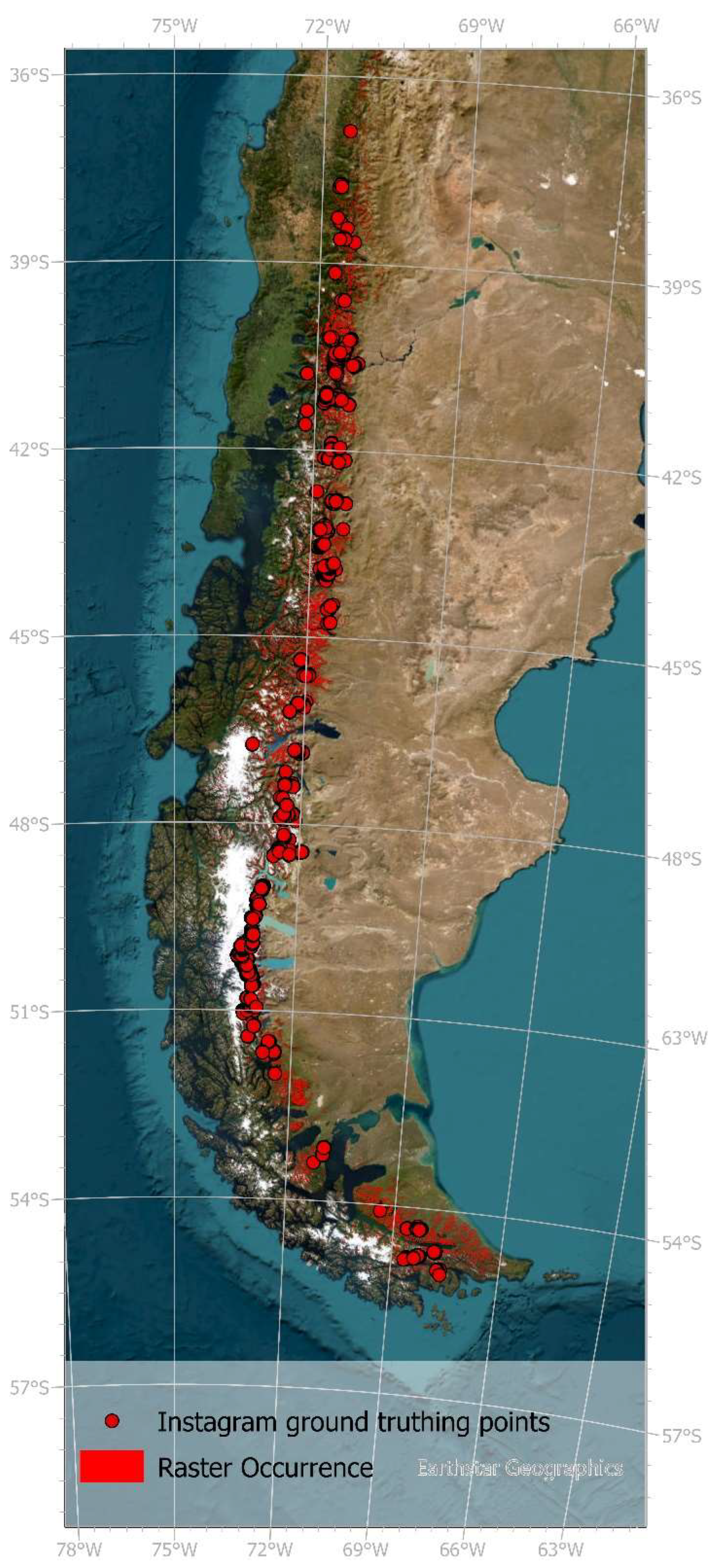
Figure 2.
Partial Dependence Plot (PDP) of (a) the Random Forest Classification and (b) Random Forest regression model indicating the influence of the most important variables.
Figure 2.
Partial Dependence Plot (PDP) of (a) the Random Forest Classification and (b) Random Forest regression model indicating the influence of the most important variables.
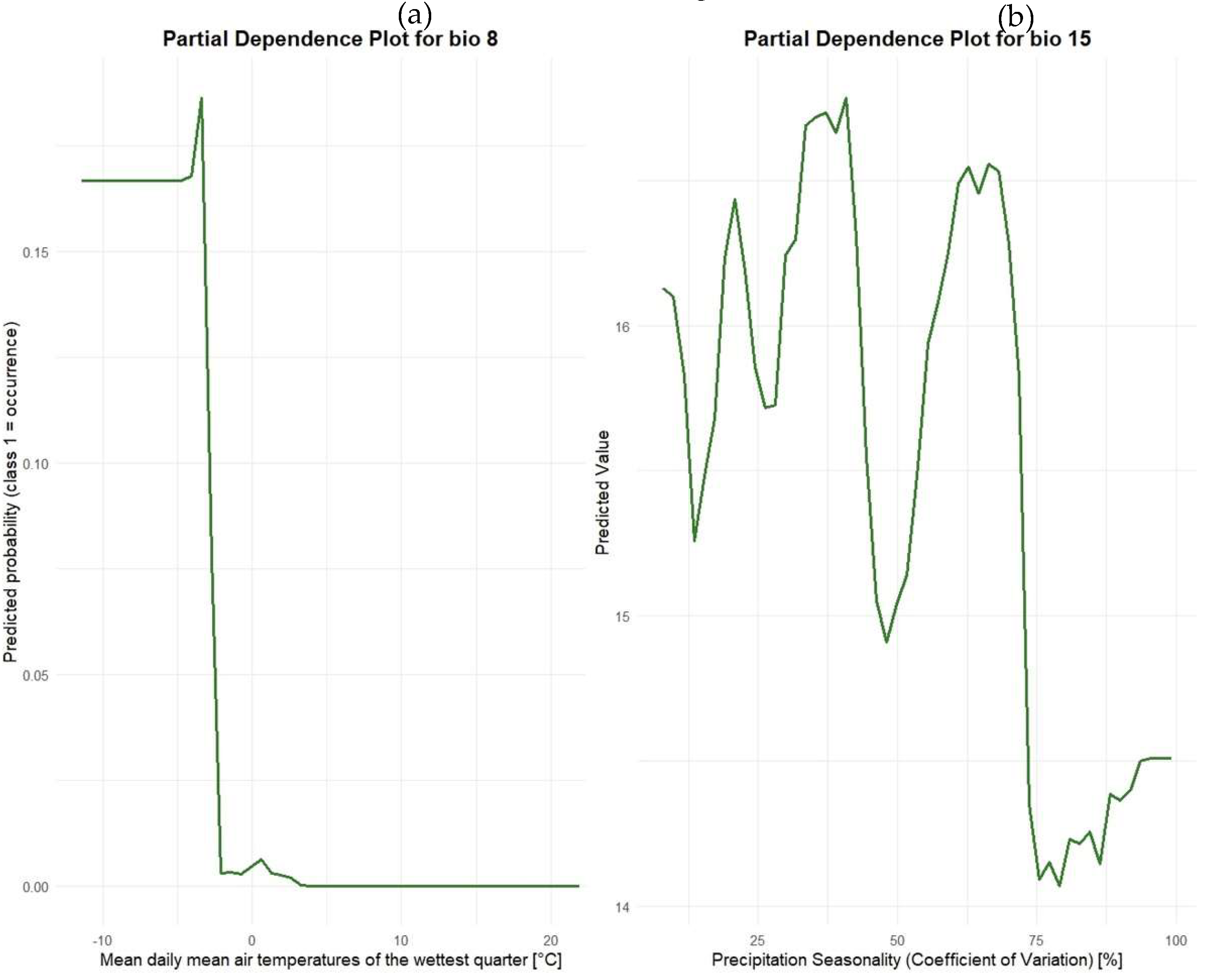
Figure 3.
Predicted probability of Nothofagus pumilio occurrence of (a) the Random Forest classification model (here abbreviated as Point model) and (b) predicted cover values of N. pumilio of the RF regression model (here Raster model).
Figure 3.
Predicted probability of Nothofagus pumilio occurrence of (a) the Random Forest classification model (here abbreviated as Point model) and (b) predicted cover values of N. pumilio of the RF regression model (here Raster model).
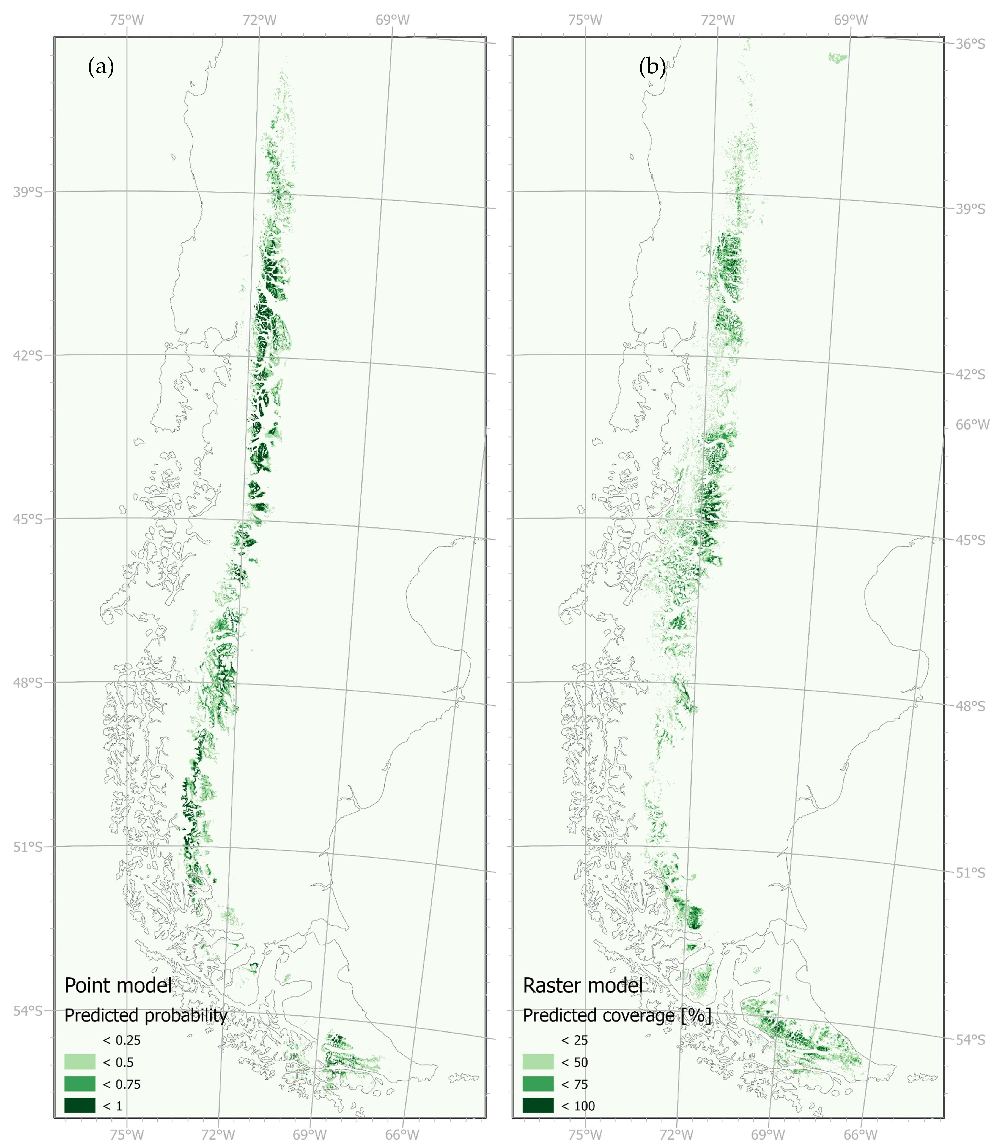
Figure 4.
Small-scale details of the Random Forest classification model (here abbreviated as Point model) and Random Forest regression model (here Raster model) compared with a satellite basemap and a Digital Surface Model (DSM), which shows the elevation of the raster cells covered by the model results.
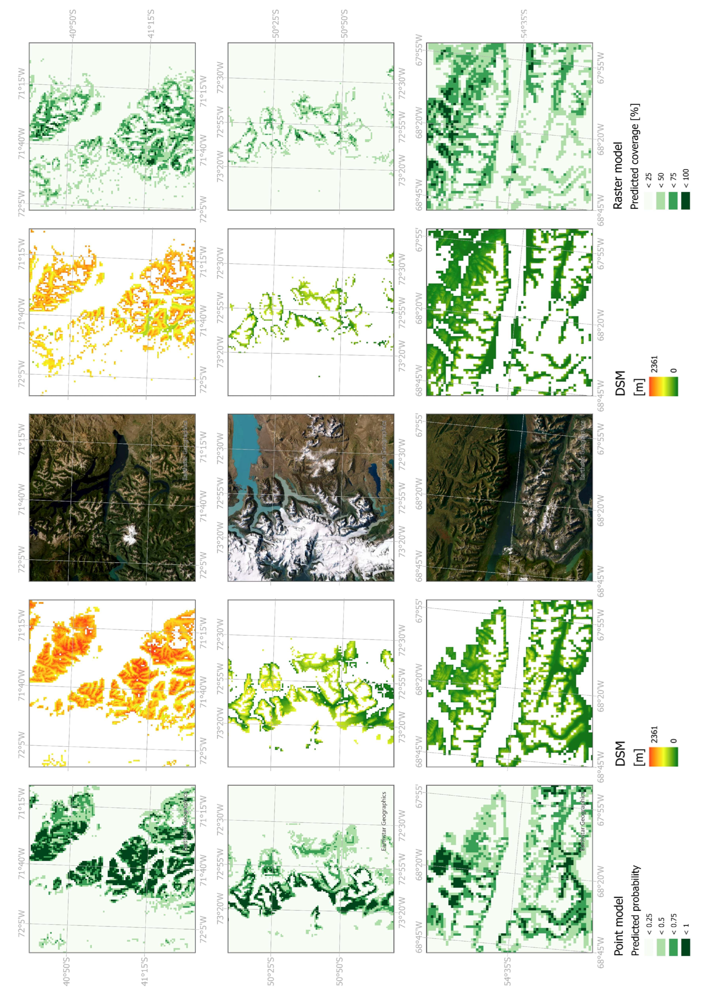
Figure 5.
Potential future distribution of Nothofagus pumilio modelled by (a) the Random Forest classification and (b) RF regression model using CMIP6 SSP Scenarios for CHELSA Bioclim variables for the time span of 2041 to 2070.
Figure 5.
Potential future distribution of Nothofagus pumilio modelled by (a) the Random Forest classification and (b) RF regression model using CMIP6 SSP Scenarios for CHELSA Bioclim variables for the time span of 2041 to 2070.
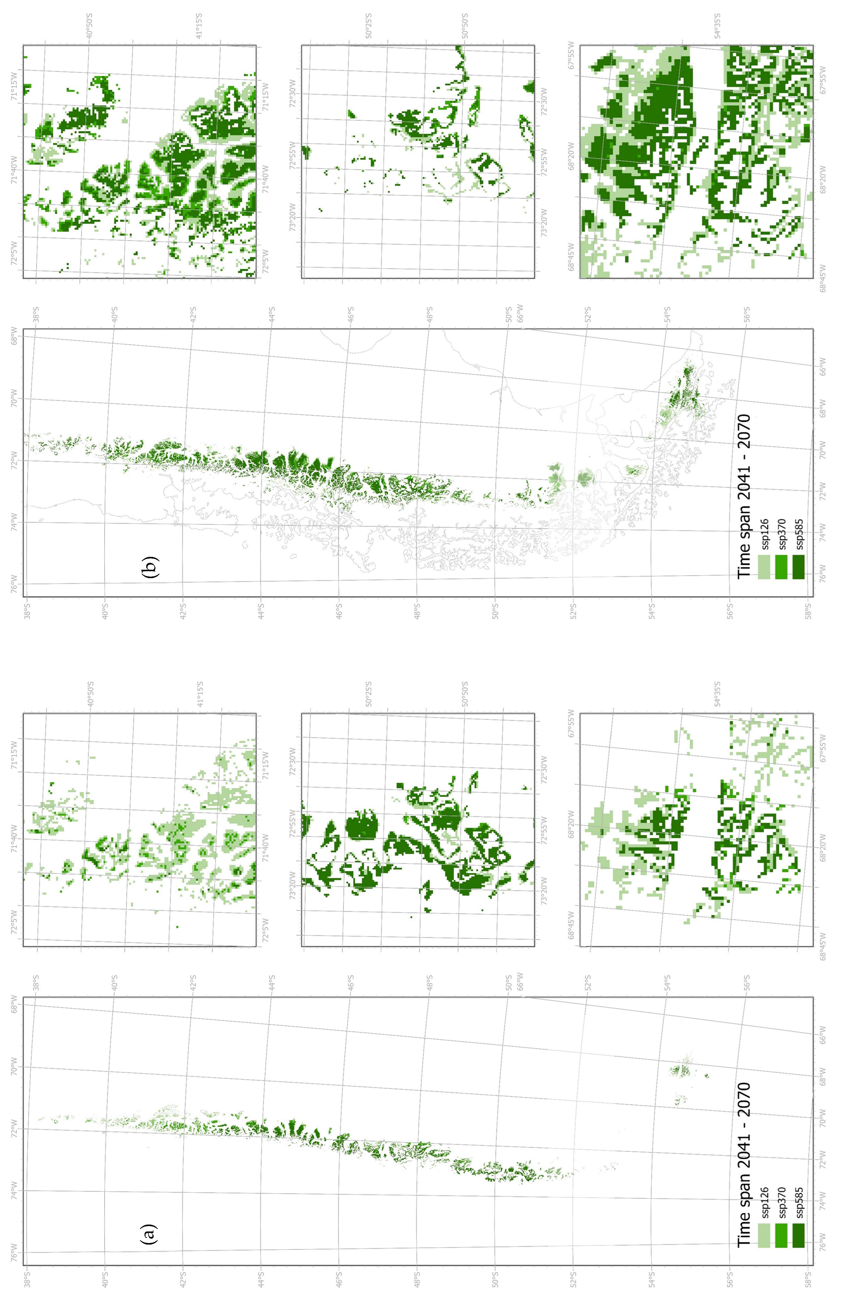
Table 1.
CHELSA Bioclim variables calculated for quarters and seasonality variables used in the analysis. The variables bio 9 and bio 16 have been excluded by the VSURF analysis.
Table 1.
CHELSA Bioclim variables calculated for quarters and seasonality variables used in the analysis. The variables bio 9 and bio 16 have been excluded by the VSURF analysis.
| Short Name | Long Name | Used in Analysis |
|---|---|---|
| bio 4 | temperature seasonality [°C/100] 1 | X |
| bio 8 | mean daily mean air temperatures of the wettest quarter [°C] | X |
| bio 9 | mean daily mean air temperatures of the driest quarter [°C] | excluded by VSURF |
| bio 10 | mean daily mean air temperatures of the warmest quarter [°C] | X |
| bio 11 | mean daily mean air temperatures of the coldest quarter [°C] | X |
| bio 15 | precipitation seasonality [kg m-2] 2 | X |
| bio 16 | mean monthly precipitation amount of the wettest quarter [kg m-2 month-1] | excluded by VSURF |
| bio 17 | mean monthly precipitation amount of the driest quarter [kg m-2 month-1] | X |
| bio 18 | mean monthly precipitation amount of the warmest quarter [kg m-2 month-1] | X |
| bio 19 | mean monthly precipitation amount of the coldest quarter [kg m-2 month-1] | X |
1standard deviation of the monthly mean temperatures; 2the coefficient of variation is the standard deviation of the monthly precipitation estimates expressed as a percentage of the mean of those estimates.
Table 2.
Predicted covered area of Nothofagus pumilio under different SSP scenarios.
| time span 2041 - 2070 | time span 2071 - 2100 | ||||
| model | area [km2] | area [%] | area [km2] | area [%] | |
| point model | SSP126 | 14916.48 | 37.54 | 14794.67 | 37.24 |
| SSP370 | 9594.11 | 24.15 | 7856.97 | 19.77 | |
| SSP585 | 11527.92 | 29.01 | 6206.62 | 15.62 | |
| raster model | SSP126 | 30143.13 | 75.06 | 28893.18 | 71.95 |
| SSP370 | 22077.23 | 54.97 | 17090.35 | 42.56 | |
| SSP585 | 27348.67 | 68.10 | 15758.20 | 39.24 | |
Disclaimer/Publisher’s Note: The statements, opinions and data contained in all publications are solely those of the individual author(s) and contributor(s) and not of MDPI and/or the editor(s). MDPI and/or the editor(s) disclaim responsibility for any injury to people or property resulting from any ideas, methods, instructions or products referred to in the content. |
© 2025 by the authors. Licensee MDPI, Basel, Switzerland. This article is an open access article distributed under the terms and conditions of the Creative Commons Attribution (CC BY) license (https://creativecommons.org/licenses/by/4.0/).
Copyright: This open access article is published under a Creative Commons CC BY 4.0 license, which permit the free download, distribution, and reuse, provided that the author and preprint are cited in any reuse.


