
Submitted:
26 May 2025
Posted:
28 May 2025
You are already at the latest version
Abstract
The trade-off between resolution and contrast is a transcendental problem in optical imaging, spanning from artistic photography to technoscientific applications. To the latter, Fourier-optics-based filters – such as the 4f system – are well-known for their image-enhancement properties, removing high spatial frequencies from an optically Fourier-transformed light signal through simple aperture adjustment. Nonetheless, assessing the contrast-resolution balance in optical imaging remains a challenging task, often requiring complex mathematical treatment and controlled laboratory conditions to match theoretical predictions. With that in mind, we propose here a simple yet robust analytical technique to find the optimal aperture in a 4f imaging system for static and quasi-static objects. Our technique employs the mathematical formalism of the H-theorem, enabling us to access directly the information of an imaged object. By varying the aperture at the Fourier plane of the 4f system, we have empirically found an optimal-aperture region where the imaging entropy is maximum, given that the object is fitted to the imaged area. At that region, the image is lit and well-resolved, and no further aperture decrease improves that, as information of the whole assembly (object plus imaging system) is maximum. With that analysis, we have also been able to investigate how the imperfections in an object affect the entropy during its imaging. Despite its simplicity, our technique is generally applicable and passable of automation, making it interesting for many imaging-based optical devices.
Keywords:
Fourier optics
; optical imaging
; applied information theory
1. Introduction
When it comes to imaging solutions, the balance between contrast and resolution is not easily achieved. In trendy fields such as super-resolution optical microscopy [1], high-resolution imaging of highly scattering media [2] and noninvasive techniques for biomedical applications [3], it is difficult to find a general configuration in which brightness and detail solving are mutually compensated given an imaged object. Therefore, different methodologies are found in the literature for the same technique in different contexts. Moreover, advancements in artificial-intelligence-based digital image processing [4] are shifting the task of handling contrast and resolution from hardware to software, as well as dealing with the modeling and explainability of real-time detections [5,6] in the place of rigid mathematical equations. Under that perspective, we decided to tackle the contrast-resolution balance problem in static and quasi-static imaging for a well-established field: Fourier optics. In particular, we were looking for an empirical approach to analyze the problem purely from the standpoint of the information carried by an image, which lead us to entropy.
In terms of image enhancement, Fourier optics has been known for decades [7] for its filtering properties, exploiting the optical Fourier transform suffered by light rays crossing a spherically surfaced lens and the removal of high spatial frequencies by adjusting the aperture of an iris diaphragm positioned at the Fourier plane of the lens. More specifically, O’Neilley and Asakura [8] in 1961 presented a formal theory connecting the information of a Fourier-transformed optical image with its formation, providing means to calculate the image-related statistical entropy H. In 1998, Kriete [9] connected entropy calculation to image quality in the context of fluorescence microscopy. Interestingly enough, few subsequent works [10] employed consistently entropic methods to assess the information of an optical images — which to us is key point for the address the contrast-resolution balance problem. As a consequence, we found no investigation about mutual contrast-resolution enhancement by optimizing the aperture at the Fourier plane — the sole degree of freedom in a Fourier-optics-based imaging system —, which motivated this study.
Our goal with this paper is twofold: (1) to present an analytical technique of practical use for experimentalists and (2) to discuss, in a heuristic manner, a different viewpoint on statistical entropy in the context of optical imaging, enabling us to understand an image as simply as the information it carries. In view of that, we discuss the H-theorem in Section 2 as a motivation for linking entropy and optical imaging in this work. In Section 3, we review the essential points about Fourier optics for understanding our experiment, whose preparation is described in Section 4. The results applying our analytical technique are then investigated in Section 5, followed by an overview of our findings in Section 6.
2. An Opto-Statistical Insight on the -Theorem
To build our intuition connecting entropy and optical imaging, we will quickly discuss the conditions and the result of the H-Theorem, following Reif’s textbook. [7] Consider an isolated system, defined by a series of approximate quantum states, where the effect of interactions is small. At any time instant t, the probability of the system being found in a particular state s is governed by the law
in which is the probability per unit time that the system makes a transition from state s to state or vice versa, a condition known as the “detailed balance.” To see what can be found from the dynamics in Eq. (1), the quantity that denotes the theorem is defined as
In the context of statistical mechanics, the quantity in Eq. (2) is regarded as the non-equilibrium entropy of the system. Notice that because , so is . Furthermore, its time derivative (which can be obtained from Eq. (1) and (2) after a few algebraic steps) gives the main result of the theorem about the dynamics of the system’s states:
Hence, will always be negative, except when all states are equally probable. In that case, the system is said to have reached equilibrium, as the entropy H attains its maximum (least negative) value, analogous to the thermodynamic potential of the same name.
As noticed by O’Neilley and Asakura [8], an image’s H as a function of the defocusing also satisfies the conditions in Eq. (3), reaching its maximum value at the focus. Therefore, H encompass information about the quality of the image somehow, which in turn is tied to both contrast and resolution. By reducing the aperture of an iris placed at the Fourier plane of a lens, one enhances the resolution by filtering higher spatial frequencies while decreasing the contrast for blocking part of the light. As a sharp image balances contrast and resolution, there should be an optimal aperture for the best image quality, maximizing the entropy of the image. The details to achieve those conditions with be analyzed in Section 3.
3. Fourier Optics and the Imaging Entropy
We recall the essential features of Fourier optics for this paper following Chapter 5 in Goodman’s textbook [11]. Consider the plano-convex lens in Figure 1 of focal length f, illuminated by a monochromatic plane-wave light source of amplitude and wavelength in the geometrical limit. For a object standing one focal length away on the left-hand side of the curved surface, the transversal electromagnetic field of the image formed at the focal point on the right-hand side of the curve surface is the Fourier transform (denoted as ) of the transversal electromagnetic field at the object’s position ( being the lens’ transference function), as shown in Eq. (4):
Note that the mapping of the incident plane wave into a focusing spherical wave in Figure 1 is reversible if we consider a point-like source at the focal point. Therefore, by mirroring the plano-convex lens into a biconvex lens and placing a copy of it two focal lengths away from the first one, we find a configuration called 4f system, which was used in the experiment described in Section 4. That arrangement allow us to Fourier-transform a signal, filter spatial frequencies of the resulting field at the focal point or Fourier plane, and then inverse-Fourier-transform the filtered signal, improving imaging.
As commented before at the end of Section 2, an iris diaphragm (often called simply iris) is placed at the Fourier plane, blocking part of the signal and thus filtering the Fourier-transformed field. The smaller the aperture (also called pupil, in contrast with the iris that blocks light), the more spatial frequencies will be removed. By modeling the aperture as , Eq. 4 informs us the U-field at the image plane of a system:
in which * is the convolution operator. Provided a static or quasi-static object, the only degrees of freedom that change come from the aperture function A. For a circular-aperture iris, it simplifies to a single degree of freedom, the aperture diameter a.
To access the information carried by , we measure the intensity of the light signal, since . Using that, O’Neilley and Asakura [8] calculated the imaging entropy as
in which p represents portions of the intensity sampled across the image plane’s photosensitive surface . Observe that Eq. (6) is mathematically equivalent to Eqs. (1) and (2). As discussed previously, the degrees of freedom to maximize H in the imaging case — thus satisfying the result of the H-theorem in Eq. (3) — comes uniquely from the aperture function A. An experiment for finding such an optimal condition is the subject of Section 4.
4. Experimental Setup
In this section, we discuss how we prepared an experiment to quantify the statistical entropy of an imaged object as a function of the optical aperture. In Section 4.1, we show the imaging system built for that purpose. In Section 4.2, we discuss the handcrafting process to make the absorptive mask used as the imaged object, called object-mask by us.
4.1. Imaging System
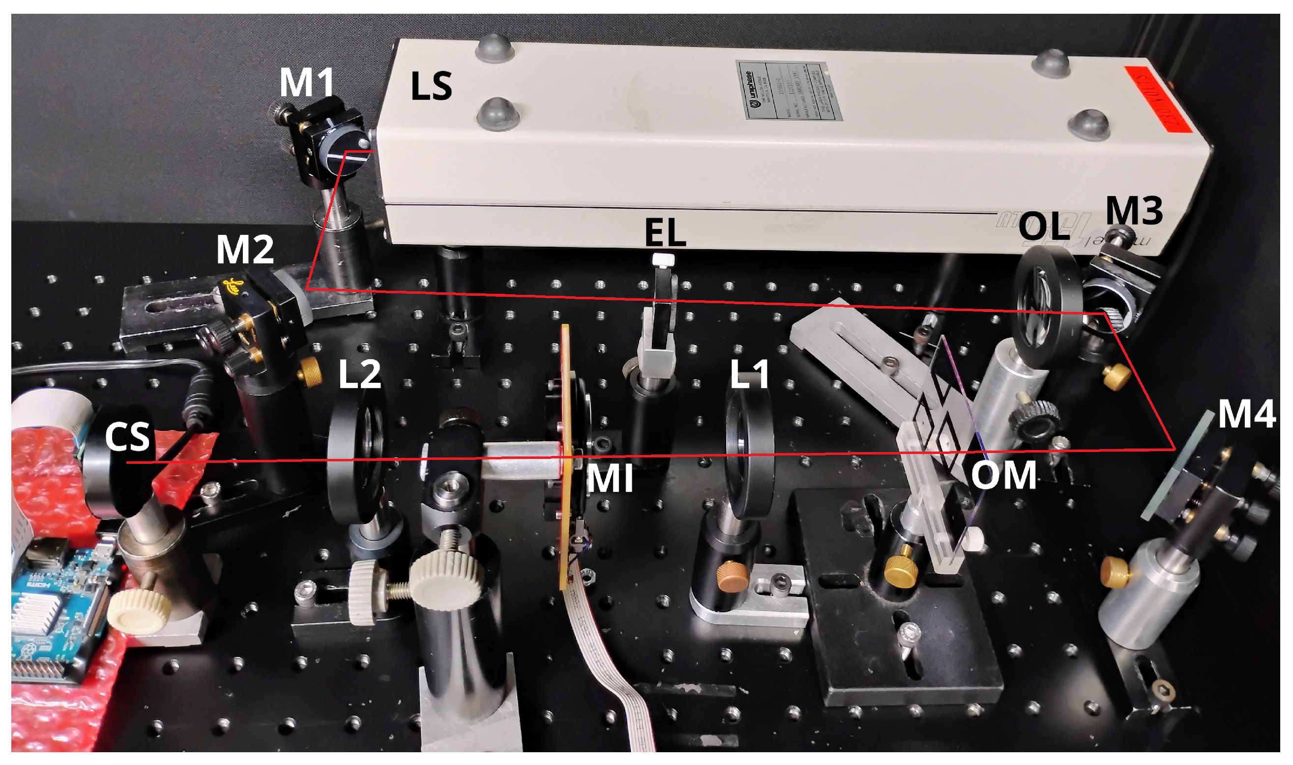
We assembled the imaging system described in Figure 2 in the corner of an optical table, surrounded by a covering structure that creates a dark environment over the table when closed. We set up this experiment for remote operation, as the object-mask (OM) remained unchanged, and the motorized iris (MI) had a cable connecting it to the control laptop, which could access the Raspberry-controlled camera sensor (CS) through a wireless link.
We set the exposition time of the camera sensor (CS) to , the shortest value for that model. We also did not lower the -mW nominal power of the laser source (LS), as we wanted to test the robustness of our analytical technique, possibly having to deal with saturated pixel values. With that in mind, we also designed a object-mask (OM) to serve as an imperfect imaged object, projecting its shadow onto CS, as explained in Section 4.2.
4.2. Object-Mask
Although originally unintended, the imperfections introduced in the object-mask shown in Figure 3 after its handcrafting process lead us to retain it to be used in our experiment. After all, measurement artifacts are present in the majority of real-world problems. Therefore, as we desire to test our method under realistic conditions, we proceeded with the measurements using that imaging target.
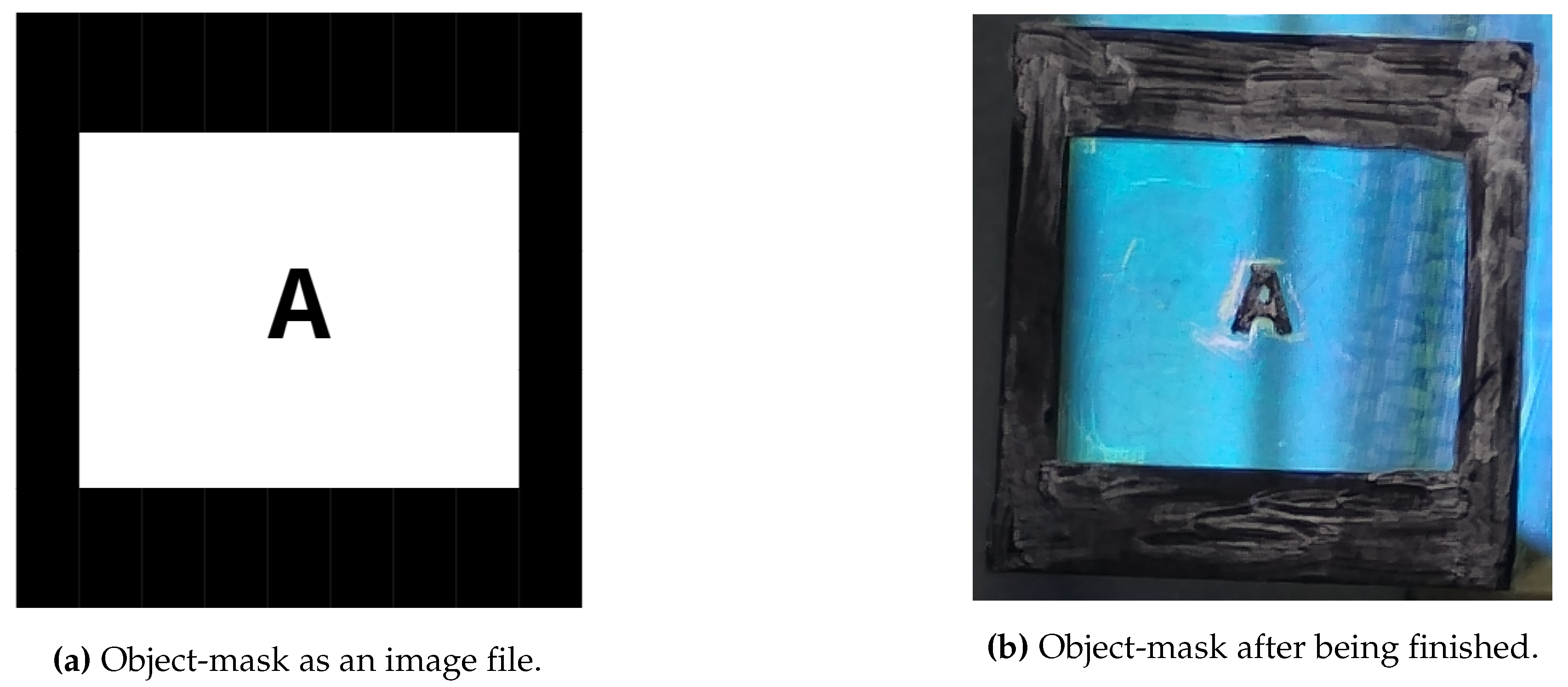
Figure 3.
A letter “A” absorptive mask used as the object-mask (OM) in the optical system of Figure 2. The design shown in (a) was initially printed on a glossy paper sheet using a high-quality printer. Then, the printed layout was cut from the sheet and placed over a piece of anti-reflective coated glass, secured by tape at the edges. Next, the paper-glass assembly was subjected to a heated press, commonly used for small-scale printed-circuit-board fabrication, to transfer the printed layout to the glass surface. However, due to the poor quality of the glossy paper, a thin layer of that material remained on the glass. That residue was manually removed using fingertip friction, which damaged parts of the print in the process. Around the letter “A”, a small file was used to avoid damaging the character itself, which in turn left scratches on the surrounding surface. Finally, a black marker pen was used to fill in the damaged areas on the print. The object-mask is seen in (b) reflecting the blue spectrum of the ceiling light, highlighting artifacts introduced during the making process, which will influence the results in Section 5.
Now the conditions of the designed experiment are known, we proceed to investigate the measurements obtained from it in Section 5, effectively applying our analytical technique.
5. Results and Discussion
From the imaging methods described in Section 4.1, we acquired 360 images of the object-mask shown in Section 4.2, with 10 images per aperture value. The acquisition started at and proceeded in steps of down to . We also acquired 10 images shot in the dark, thus capturing the background noise. In Section 5.1, we present how we did the post-processing of those images. In Section 5.2, we show how the statistical entropy H of each image was obtained, followed by an inspection of the diagrams in Section 5.3, allowing us to find the optimal-aperture region.
5.1. Image Post-Processing
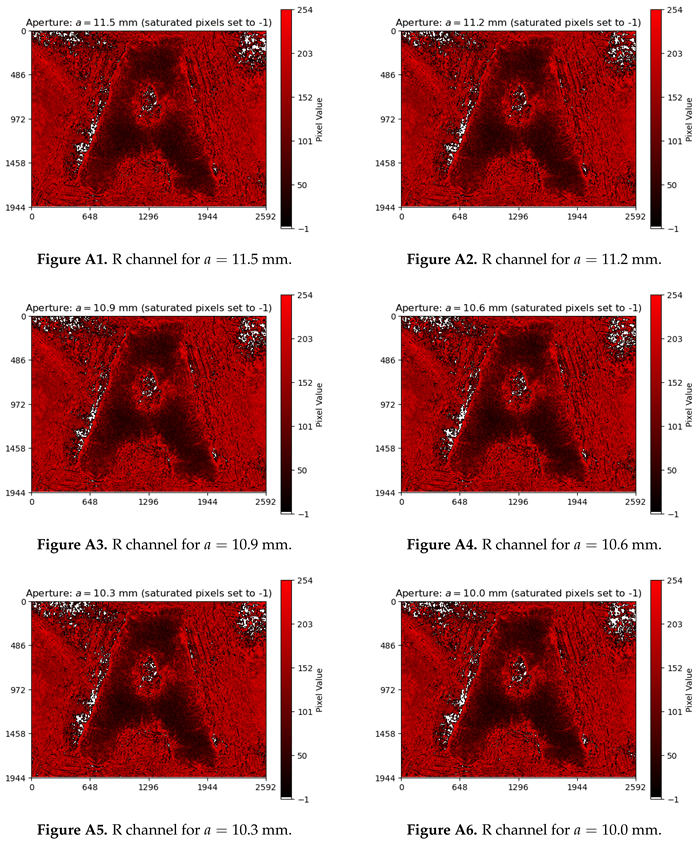
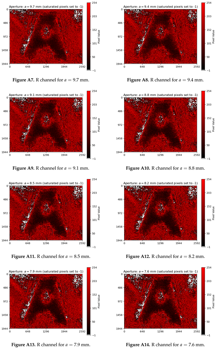
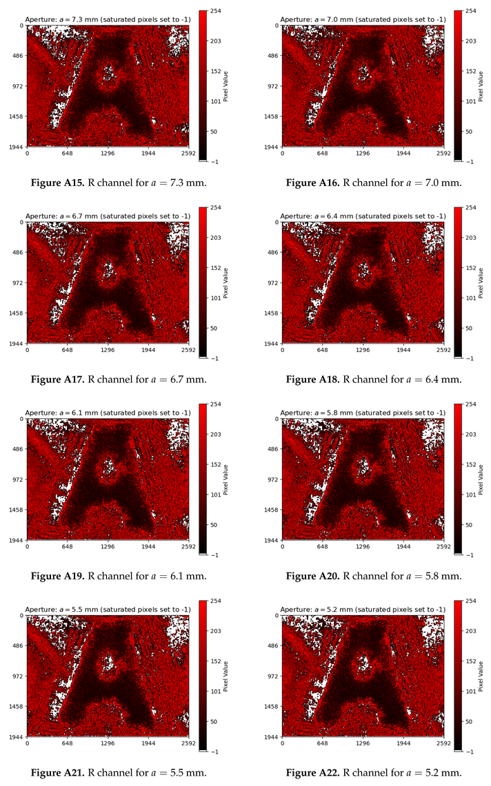
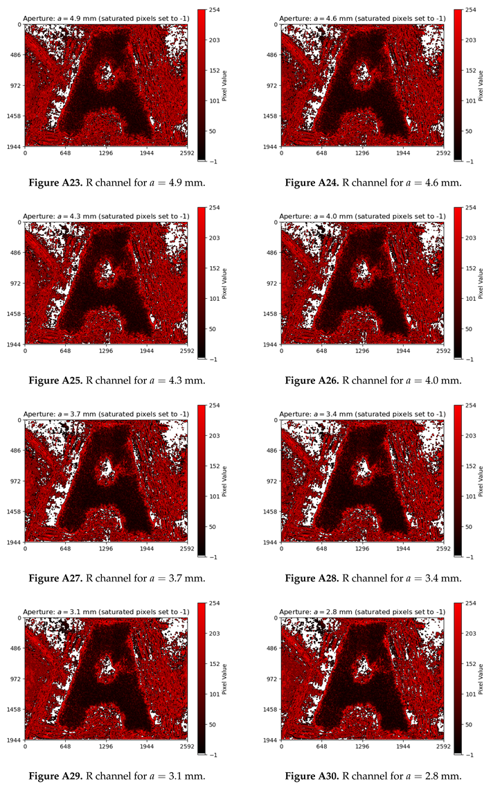
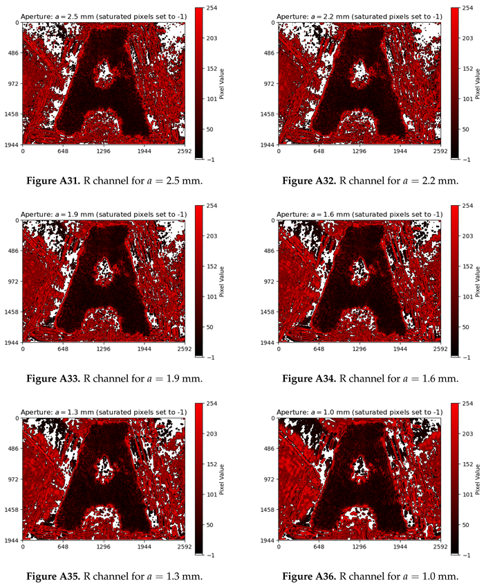
Each image file is represented as a tensor, corresponding to the three color channels (RGB) and the pixel arrays captured by the camera sensor for each color. As the laser wavelength was nm, we used only the R-channel data, converting the images into pixel matrices, whose values ranged between 0 and 255. We computed the definitive image as the mean (-matrix) with its standard deviation (-matrix) of the 10 acquired images, resulting in two characteristic matrices for each aperture. For saturated and high-variance () pixels in the -matrix, their values were assigned to , excluding them from the calculations in Section 5.2. To distinguish between viable and unviable pixels in the -matrices (i. e. the definitive images), we created a custom color map, setting as white, 0 as black and 254 as red, as shown in Figure 4. The full list of 36 final images is presented in Appendix A – again, one image per aperture value.
Figure 4.
Selected images from Appendix A for analyzing the diagrams in Figure 5 and Figure 6: the highest-aperture (a) and the lowest-aperture (b) images above the transition region, and the highest-aperture (c) and the lowest-aperture (d) images below the transition region. Saturated and high-variance pixels are not used for entropy calculations in Section 5.2.
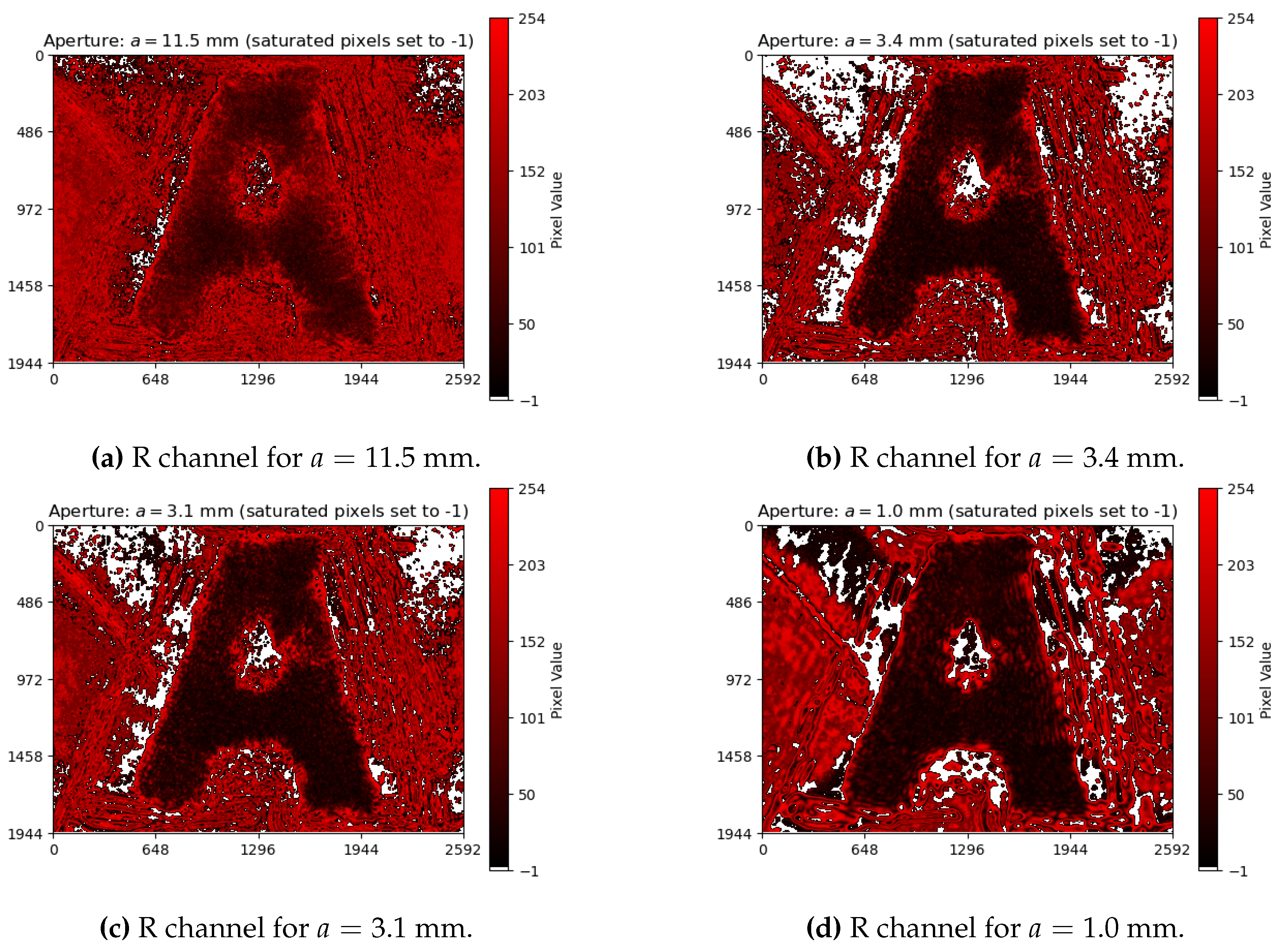
The sequence of images in Figure 4 displays how the features defining the letter “A” become more distinguishable as the aperture is reduced, although making them darker. Moreover, imperfections in the object-mask also become more evident at smaller apertures – artifacts that will be considered later on our analysis. Those images will be revised when we analyze the behavior of the entropy, whose calculation is described in Section 5.2.
5.2. Entropy Calculation
To calculate the entropy of each image, we adopted the following procedure:
After the steps above, each -matrix representing an image becomes effectively a table of portions segmenting the image, as intended in Eq. (6). However, as the normalized pixel values are very small, computing their logarithms can be hard. Thus, we used this method:
- Take the absolute order of magnitude of the smallest pixel value: .
- Calculate the logarithms as
With the entropy determined, we examine its dependency on the aperture in Section 5.3.
5.3. Entropy-Versus-Aperture Diagrams
To investigate the statistical quality of the collected data, we filtered the pixel values from the - and -matrices – between the procedures from Section 5.1 and Section 5.2 – to retain only those satisfying selected thresholds for the coefficient of variation, , such that the ratio was less than or equal to the specified values. This allows us to observe how robust the overall behavior of entropy as a function of aperture remains as the coefficient-of-variation threshold for pixels is progressively reduced. Therefore, the diagrams for selected curves are shown on a linear scale in Figure 5 and on a log-log scale in Figure 6.
Figure 5.
Behavior of the entropy as a function of the aperture for the images of the object-mask in Figure 3, that were acquired with the imaging system in Figure 2. The curves retain their overall shapes for coefficient-of-variation thresholds up to 0.2, indicating the limit of statistical reliability. There is a clear change in the behavior of the curves between mm and mm (orange-shaded area), marking the region of optimal aperture for the best trade-off between resolution and contrast.
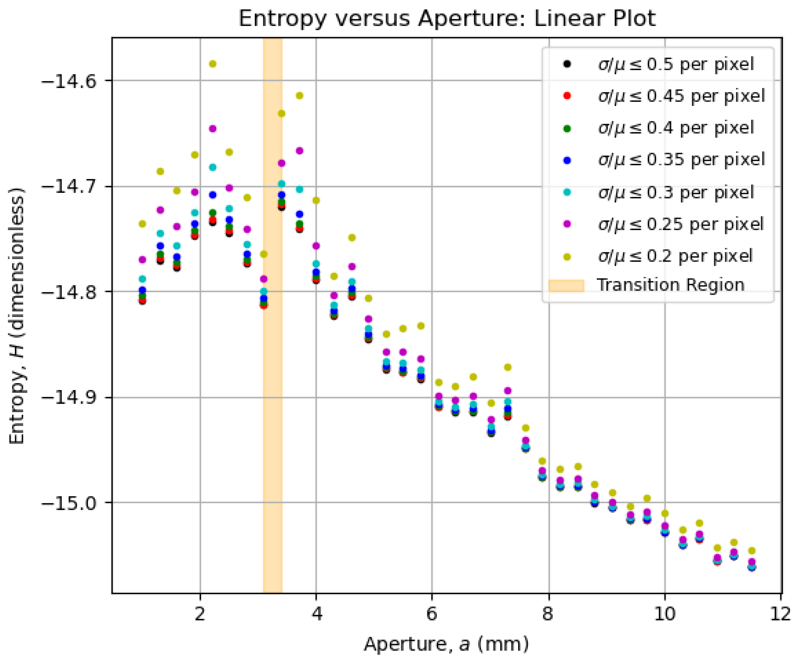
We highlighted in Figure 5 and Figure 6 an orange-shaded region that marks an abrupt change in the behavior of the curves, which we refer to as the “transition region”. For apertures mm (above the transition region), the entropy was calculated from all images between Figures 4(a-b), whereas for apertures mm (below the transition region), the the entropy was determined from all images between Figures 4(c-d). We will analyze the regions above and below the transition area in the following paragraphs, arguing that the aperture values within the transition region offer a robust compromise between contrast and resolution, improving significantly the imaging conditions.
Figure 6.
Log-log-scale version of the diagram in Figure 5, in which the smoothening effect of the logarithm function on the curves makes their behavior more evident. Note how little the data varies for apertures below the transition region, pointing at an expected stability below the optimal aperture.
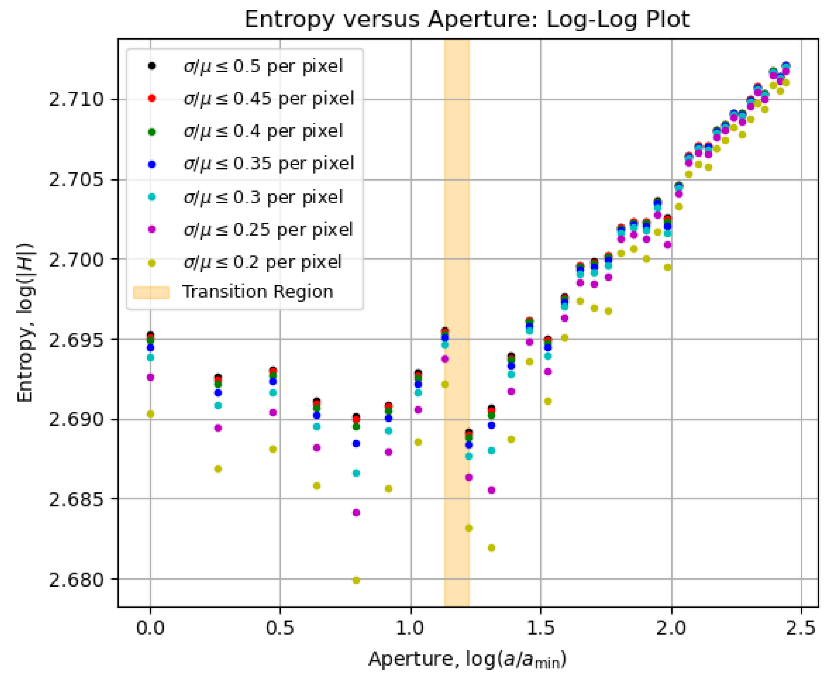
Above the Transition Region
For apertures bigger than an expected optimal value, the entropy increase can be approximated to a straight line on a logarithmic scale, as seen in Figure 6. That growth behavior is a characteristic feature of the assembly constituted by the imaging system and the imaged object, and it can be used as a reference for determining the transition region for quasi-static scenarios (e. g. slow chemical reactions on a slide as the imaged object). In terms of content, the smaller the aperture, the greater is the information about the object – as observed between Figures 4(a-b), with the details of the letter “A” becoming sharper. That information however is ultimately limited at the transition region, given an imaged object.
Below the Transition Region
At first glance, it might seem inappropriate to assume that the entropy reaches its maximum stable value by looking at Figure 5 and Figure 6. However, if we look at Figures 4(c-d), dark patches around the letter “A” started to appear and become more evident as the aperture decreases. These dark patches are imaging artifacts introduced by the imperfections on the object-mask, as commented in Figure 3. The smaller the aperture, the lower the contrast and the higher the resolution, thus the imperfections – previously neglectable – become evident, influencing the entropy values below the transition region.
Note that our analysis assumes all relevant structural information about the object – specifically, the letter “A” on the object-mask – is fully contained within the imaged area, and that no additional structures beyond the letter are of interest. If, instead, one wished to image finer details of the print itself, the imaging system would need to be adjusted – such as by increasing magnification – to appropriately capture the desired structural features. For that reason, the entropy for the letter “A” image reached its maximum value at the transition region, where one finds an optimal aperture value, balancing contrast and resolution.
6. Conclusions
In this paper, we have described an analytical technique for measuring the statistical entropy of an imaged object as a function of the imaging system’s aperture, enabling the identification of an aperture value that optimizes resolution and contrast to yield a detailed and well-illuminated image. Our approach draws inspiration from the premises of the H-theorem, which explains how certain nonequilibrium systems evolve towards equilibrium, while employing the spatial filtering properties of Fourier optics.
As a case-study of our technique, we have built a system to image an object-mask with imperfections, as discussed in Section 4. We have imaged that target at various aperture values, determining the entropy of each image, as presented in Section 5. We have found a transition region where the entropy as function of the aperture changes its behavior. Above that region, entropy increases as aperture decreases. Below that region, details from the imperfections become evident, affecting the entropy curve. Therefore, the transition region is where the optimal aperture is, with the intended details of an object in evidence.
On one hand, an important assumption for our technique is that the desirable information about an imaged object is fitted into the imaged area. Smaller structures within that area might not be as resolved as the structures that fill the characteristic dimensions under imaging. Furthermore, it also assumes a static or quasi-static target at the object plane.
On the other hand, our analytical technique has the advantage of not relying on heavy mathematical modeling and physical treatment, as many other approaches usually do. In fact, it relies mainly on the content that comes with the definition of entropy, making it a very robust method for optical imaging enhancement. In terms of applications, this technique does require aperture scanning; however, this requirement enables automated optimization, making it particularly attractive for improving optical scanners, confocal microscopes, and other Fourier-optics-based systems.
Author Contributions
Conceptualization, M.M. and D.V.M.; methodology, M.M.; software, M.M.; validation, M.M.; formal analysis, M.M.; investigation, M.M.; resources, D.V.M.; data curation, M.M.; writing—original draft preparation, M.M.; writing—review and editing, M.M.; visualization, M.M. and D.V.M; supervision, D.V.M.; project administration, D.V.M.; funding acquisition, D.V.M. All authors have read and agreed to the published version of the manuscript.
Funding
This research received no external funding.
Institutional Review Board Statement
Not applicable.
Informed Consent Statement
Not applicable.
Data Availability Statement
The minimum dataset was provided with the submission. The full dataset is available upon request due to file size limitations.
Acknowledgments
The authors are grateful for the thoughtful discussions with Prof. Sebastião Pratavieira and Prof. Sérgio Ricardo Muniz, who introduced the first author to the fascinating concept of Fourier optics, thus inspiring the work presented in this article.
Conflicts of Interest
The authors declare no conflicts of interest.
Appendix A. Images
We present here the full list of the images taken for our analysis, following the procedures from Section 4 and Section 5. Figures A1-A36 represent the shadow of the letter “A” mask in Figure 3 projected onto the camera sensor after crossing the system seen in Figure 2, for different aperture values. Their post-processing is described in Section 5.1.
References
- Prakash, K.; Baddeley, D.; Eggeling, C.; Fiolka, R.; Heintzmann, R.; Manley, S.; Radenovic, A.; Smith, C.; Shroff, H.; Schermelleh, L. Resolution in super-resolution microscopy—definition, trade-offs and perspectives. Nature Reviews Molecular Cell Biology 2024, 25, 677–682. [Google Scholar] [CrossRef] [PubMed]
- Bertolotti, J.; Katz, O. Imaging in complex media. Nature Physics 2022, 18, 1008–1017. [Google Scholar] [CrossRef]
- Wang, D.; Sahoo, S.K.; Zhu, X.; Adamo, G.; Dang, C. Non-invasive super-resolution imaging through dynamic scattering media. Nature communications 2021, 12, 3150. [Google Scholar] [CrossRef] [PubMed]
- Lepcha, D.C.; Goyal, B.; Dogra, A.; Sharma, K.P.; Gupta, D.N. A deep journey into image enhancement: A survey of current and emerging trends. Information Fusion 2023, 93, 36–76. [Google Scholar] [CrossRef]
- Pushkina, A.; Maltese, G.; Costa-Filho, J.; Patel, P.; Lvovsky, A. Superresolution linear optical imaging in the far field. Physical review letters 2021, 127, 253602. [Google Scholar] [CrossRef] [PubMed]
- Fu, T.; Zhang, J.; Sun, R.; Huang, Y.; Xu, W.; Yang, S.; Zhu, Z.; Chen, H. Optical neural networks: progress and challenges. Light: Science & Applications 2024, 13, 263. [Google Scholar]
- Reif, F. Fundamentals of Statistical and Thermal Physics; McGraw-Hill, 1965.
- L. O’Neill, E.; Asakura, T. Optical image formation in terms of entropy transformations. Journal of the Physical Society of Japan 1961, 16, 301–308. [Google Scholar] [CrossRef]
- Kriete, A. Image quality. Journal of Computer-Assisted Microscopy 1998, 10, 167–171. [Google Scholar] [CrossRef]
- Stimper, V.; Bauer, S.; Ernstorfer, R.; Schölkopf, B.; Xian, R.P. Multidimensional contrast limited adaptive histogram equalization. IEEE Access 2019, 7, 165437–165447. [Google Scholar] [CrossRef]
- Goodman, J.W. Introduction to Fourier Optics; McGraw-Hill, 1968.
Figure 1.
The curved surface of a thin plano-convex lens maps an incident plane wavefront into a spherical wavefront. By placing a point source on the focal point and flipping the curved surface towards it, the curved surface now maps the incident spherical wavefront into a plane wavefront. Source: https://commons.wikimedia.org/wiki/File:Spherical_wave_lens2.svg (CC BY-SA 3.0).
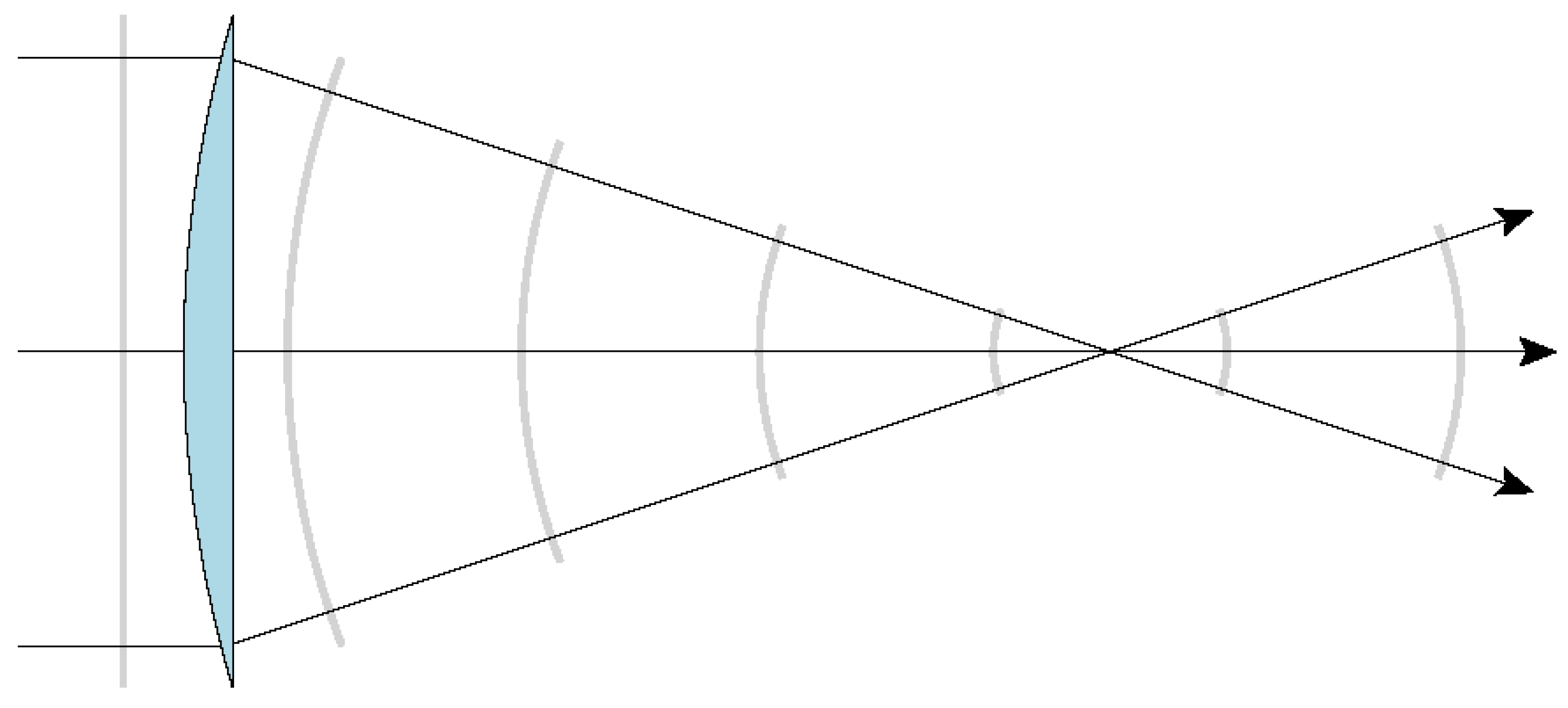
Figure 2.
Optical system assembled for our experiment. The red-line segments indicate the path of the light throughout the system, which was produced by a -nm helium-neon laser source (LS) and whose height and slope of the laser beam was precisely controlled by a set of four aluminum mirrors (M1, M2, M3 and M4). Between M2 and M3, a Keplerian telescope was set up, using an eyepice lens (EL) of mm an objective lens (OL) of mm, producing a collimated beam of approximately 1 cm in diameter at the back of OL. That collimated beam was guided by M3 and M4 to a system using two biconvex lenses (L1 and L2) of mm. At the object plane, the object-mask (OM) shown in Figure 3 was positioned, imprinting a letter “A” on the beam as a shadow. At the Fourier plane (where L1 and L2´s focci coincide), a remotely operable motorized iris (MI) was placed for aperture control. At the image plane, a camera sensor (CS) was settled: a lensless 5-megapixel camera module connected to a Raspberry board (partly visible at the lower left corner).
Disclaimer/Publisher’s Note: The statements, opinions and data contained in all publications are solely those of the individual author(s) and contributor(s) and not of MDPI and/or the editor(s). MDPI and/or the editor(s) disclaim responsibility for any injury to people or property resulting from any ideas, methods, instructions or products referred to in the content. |
© 2025 by the authors. Licensee MDPI, Basel, Switzerland. This article is an open access article distributed under the terms and conditions of the Creative Commons Attribution (CC BY) license (http://creativecommons.org/licenses/by/4.0/).
Copyright: This open access article is published under a Creative Commons CC BY 4.0 license, which permit the free download, distribution, and reuse, provided that the author and preprint are cited in any reuse.


