Submitted:
27 July 2025
Posted:
28 July 2025
Read the latest preprint version here
Abstract
We present a formal reconstruction of the conventional number systems, including integers, rationals, reals, and complex numbers, based on the principle of relational finitude over a finite field \( \mathbb F_p \). Rather than assuming actual infinity, we define arithmetic and algebra as observer-dependent constructs grounded in finite field symmetries. Conventional number classes are then reinterpreted as pseudo-numbers, expressed relationally with respect to a chosen reference frame. We define explicit mappings for each number class, preserving their algebraic and computational properties while eliminating ontological dependence on infinite structures. For example, pseudo-rationals emerge from dense grids generated by primitive roots, enabling proportional reasoning without infinity, while scale-periodicity ensures invariance under zoom operations, approximating continuity in a bounded structure. The resultant framework---that we denote as Finite Ring Continuum---establishes a coherent foundation for mathematics, physics and formal logic in ontologically finite paradox-free informational universe.
Keywords:
finite fields
; modular arithmetic
; relativistic algebra
; symmetry transformations
; pseudonumbers
; observer framing
; discrete manifolds
; approximate lie groups
; finite informational systems
; structural mathematics
; modular exponentiation
; cyclic groups
; finite field morphology
; relational symmetries
; epistemic construct
1. Introduction
A growing body of work in mathematics and physics suggests that foundational structures are best understood through a relational or relativistic lens [1,2,3]. In such a paradigm, mathematical entities acquire meaning not as intrinsic absolutes but through their role within a system defined by internal symmetries and reference frames. Constants like 0, 1, or i are not metaphysical primitives, but relational markers—origins, units, or axes—assigned by a chosen framing.
This perspective invites a re-evaluation of one of the most entrenched assumptions in mathematics: the acceptance of actual infinity. From real analysis to Hilbert spaces, infinity has been treated as foundational, despite its lack of empirical or computational realization. Under a relational view, such constructs may instead be interpreted as emergent limits or symbolic artifacts—arising when finite systems attempt to encode relationships that exceed their internal scope.
In previous work [4], we argued that concepts like infinity, randomness, and undecidability are not ontological features of nature, but epistemic placeholders—signals of representational saturation in finite informational systems. Here, we extend this view into a concrete formalism: a relativistic algebra constructed entirely over a finite field , with observer-relative arithmetic and emergent pseudo-numbers.
This relational paradigm finds a natural analogue in the development of modern physics. The transition from Newtonian mechanics to Einsteinian relativity redefined the very notions of space, time, and simultaneity—not as absolute quantities but as frame-dependent observations shaped by internal consistency and symmetry. Likewise, a relativistic mathematics replaces external absolutes with internal coherence, viewing all mathematical structures and operations as inherently contextual, subject to transformation, and defined through symmetry relations within finite systems. Such a shift enables a more consistent and physically meaningful foundation for mathematics, especially in the domain of closed, informationally finite systems. It offers a unified perspective that bridges abstract algebra, geometry, and modern physical theory, and sets the stage for a reconstruction of mathematical reasoning grounded in self-contained, finite, and relational structures.
The present framework resonates with several contemporary perspectives that question the ontological status of the continuum and advocate for finitely constructed alternatives. In particular, Smolin has emphasized the need for a relational, observer-dependent formulation of physical laws, suggesting that the continuum is merely an idealization beyond the reach of internal observers [5,6]. Lev provided a comprehensive treatment of finite mathematics as a foundation for quantum theories [7] showing that the classical mathematics can be regarded as a special degenerate case of the finite mathematics. Similarly, D’Ariano and collaborators have reconstructed quantum theory from finite, informationally grounded axioms, demonstrating that core features of quantum mechanics can emerge without invoking infinite-dimensional Hilbert spaces [8]. From a mathematical standpoint, the approach aligns with the ultrafinitist program developed by Benci and Di Nasso, which offers a rigorous alternative to classical cardinality through the theory of numerosities and bounded arithmetic [9,10].
Furthermore, the ultrafinitist school—pioneered by Yessenin-Volpin and Parikh—takes finitude even further by denying the meaningful existence of “too large” numbers and insisting on feasibility as a foundational constraint. Formalizations of ultrafinitism and feasibility arithmetic appear in works such as [11,12,13,14], which explore the proof-theoretic and computational consequences of enforcing strict constructive bounds on arithmetic.
Ultrafinitism enforces an a priori cutoff on numerical existence—only those magnitudes deemed “feasible” within a human or machine resource bound are admitted. By contrast, our relativistic framework treats finiteness not as a hard barrier but as a contextual framing condition: We allow arbitrarily large numbers, so “size” is always relative to the chosen frame. Infinite structures, such as integers and rationals emerge asymptotically or as coordinate projections, rather than being forbidden. Arithmetic operations become internal symmetries of a finite system, rather than operations constrained by external feasibility checks. This shift replaces the ultrafinitist’s absolute feasibility threshold with a relational notion of scope: any number “exists” within some finite frame, while “infinity” itself appears as a relative point beyond the horizon of observability and algebraic accessibility.
To illustrate, consider an observer on the surface of the planet Earth perceiving an infinite flat plane (as they indeed do) conveniently centred around their exact position. This is not just epistemic error, but an ontological misinterpretation of the true structure, that is the large but finite, curved sphere. While the “flat Earth” paradigm may appear outdated to most modern audience, other egocentric models such as the geocentricity and heliocentricity are relatively recent, while the “infinite flat” universe model remains the prevailing cosmological framework. Similarly, classical infinite numbers with an absolutely defined origin 0 and scale 1 can be identified as an egocentric mathematical paradigm that approximates the modular closure of the large but finite, modular arithmetic in an information horizon-constrained frame of reference that is relative to the observer. The round Earth metaphor is a concrete example of how finiteness and infinity can be reconciled through relational, modular framing, as detailed in [7].
To support this framework, we further draw upon several key developments in mathematics and physics. The foundational critique of actual infinity has been explored in works such as [15,16], which emphasize the constructive and finitist approaches to mathematics. The relational perspective on mathematical objects aligns with category theory [1], where objects are defined by their morphisms and relationships rather than intrinsic properties. Additionally, the parallels between relativistic mathematics and modern physics are inspired by the symmetry principles in [2,3], which highlight the role of invariance and frame-dependence in physical laws. Finally, the informational limits of finite systems and their implications for mathematical representation are discussed in [17,18].
The present article forms the algebraic foundation of a three-part programme designed to reconstruct the familiar continuous structures from finite arithmetic using the framework of Finite Ring Continuum (FRC) as depicted in Figure 1. The present work, Algebra, establishes a relational framing of the classical number hierarchy () as pseudo-number classes within a single finite field, demonstrating that all constructions are covariant under a change of arithmetic frame. The subsequent paper, Geometry, lifts this algebraic structure to a pseudo-smooth two-sphere with constant internal curvature, from which canonical geometric constants are derived. The final manuscript, Composition, extends the framework from prime to composite moduli using the Chinese Remainder Theorem, yielding a bouquet of prime spheroids whose structure resembles a Seifert-fibred three-orbifold. This modular presentation ensures that each layer is developed with incremental and verifiable rigour.
2. Reference Frame in Finite Field
Let be a finite field of integers modulo a prime , where is a natural number1. The elements of form a complete and closed set of relational representations of under modular addition, multiplication, and exponentiation. However, the specific numeric labels assigned to these elements—particularly the designation of 0 and 1 as the additive and multiplicative identities—are intrinsically relative and carry no absolute meaning within the field itself. The field is invariant under relabelling of its elements via any bijective affine transformation of the form
where and . Such transformations preserve the field structure and allow any element to be reinterpreted as an origin. In this sense, the element labelled 0 is not uniquely privileged; it simply represents the additive identity with respect to a chosen reference frame. The same applies to the label 1, which identifies the multiplicative unit only relative to a particular scaling.
Definition 1
(Affine Reference Frame). An affine reference frame in consists of picking two distinguished elements
and then defining relabelled addition and multiplication by
where divisions are in the original field .
Lemma 1
(Affine Ring Isomorphism). Let be a finite field, and let two frames and be related by the affine bijection
Then ϕ is a ring isomorphism between and . Consequently, any polynomial identity
if and only if the “relabelled” identity
where .
Proof.
Since , is a bijection with inverse . For any ,
and similarly
Thus, preserves addition and multiplication, so it is a ring isomorphism. It follows immediately that any algebraic (polynomial) relation valid in one frame is carried over to the other by conjugation with , establishing frame-independence of all algebraic identities. □
Therefore, in the absence of an externally imposed or contextually declared frame—such as one defined by a designated pair —the labels in are relational rather than absolute. Ontologically, this means that numerical identity is an observer-dependent convention rather than an intrinsic property of the set, so the passage from one frame to another is not merely an algebraic relabelling but a shift in perspective. The roles of “zero” and “one” are thus not the fundamental properties of the elements themselves, but a consequence of the system’s framing, making all representations in symmetric and interchangeable under coordinate transformation. To define our system unambiguously, we must specify a reference frame or coordinate system within the context of , which then becomes a framed finite ring .
A typical diagram of a framed finite field , where , is shown in Figure 2. We would like to specifically note that such a diagram is typically visualised as a circle on a 2D plane spanned by the radial axis and rotational symmetry under the arithmetic operation of addition, thus assigning an intuitive geometric interpretation to the arithmetic structure of the additive group . We will henceforth assume all such systems to be framed systems and will denote the corresponding finite ring as for simplicity, unless explicitly stated otherwise.
3. Finite Field as Discrete Geometric Structure
Let be a prime and let denote the finite field with elements [21]. The association between arithmetic operations and symbolic geometry detailed in Section 2 can be extended further. Specifically, in the finite field , the basic arithmetic operations of counting, addition, multiplication, and exponentiation can be all understood as manifestations of the underlying symmetries of structural transformations of the field [22].
Counting corresponds to the selection of the next element of the foundational parameter :
While typically taken for granted, the act of counting is an ontologically and informationally significant degree of freedom that both presupposes the existence of the field , and determines the entirety of its structural properties. Furthermore, the counting operation establishes a translation symmetry successor maps and that underpin all other arithmetic operations as its iterative applications.
Addition (translation) corresponds to the iterative application of counting. The additive group forms a finite cyclic group of order , generated by the element 1. Translation symmetry is defined by additive shifts:
This operation reflects the periodic structure of the ring, and can be viewed as a rotation by a steps around the absolute origin (see Figure 2) and the corresponding circular configuration of the elements of .
Multiplication (scaling) corresponds to the iterative application of addition, and furthermore reflects the scaling symmetry within the field. Scaling symmetry is defined by multiplicative operation
and corresponds to a dilation or contraction of the additive structure, where the effect of multiplication is constrained by the modulus.
Exponentiation (powering) is an iterative application of multiplication defined by the modular operation
where is a finite ring of the order , which is importantly no longer a field. This operation defines power maps and automorphisms that reveal the group-theoretic structure and internal symmetries of the field, and encodes deep number-theoretic properties such as primitive roots and residue classes [21].
Thus, the basic arithmetic operations in are not arbitrary—they are algebraic expressions of the field’s internal symmetries. They define how elements of the system transform under structured, invertible actions, and they reveal the harmonious regularity inherent in finite arithmetic.
Proposition 1
(3-Manifold Geometry of ). For a fixed value of the foundational parameter , the framed finite field , together with its triplet of arithmetic symmetries, may be interpreted as a discrete symbolicthree-dimensional manifold embedded in an abstract four-dimensional symmetry space .
Consider a symbolic symmetry space , where all geometric objects, such as vertices, edges and faces, are defined relative to each other and the observer’s frame of reference, in the exact same way as the elements of the field in Figure 2 are defined by nothing else than their relation to each other and the observer’s frame of reference. Each vertex in corresponds to a specific element in , but the finite number of elements of the field can be repeated arbitrary many times in .
Remark 1
(Kaliedoscope Metaphor). Here, we would like to offer the metaphor of a kaleidoscope, where a relatively small set of physical elements generates an arbitrary large and seemingly-complex pattern via reflections and symmetries. The emergent patterns are dependent on the observer’s frame of reference, and the same set of elements can generate different patterns for different observers.
Definition 2
(Carrier hyper-cube). Define thecarrier hyper-cube as a symbolic space defined by 4-tuples comprising a fixed value of and all possible values of parameters in
Definition 3
(Symmetry space). Thesymmetry space is defined as the quotient of the carrier hyper-cube by the action of the symmetry group generated by the three arithmetic operations relative to the selected frame of reference . As such, resides in the category of finite sets (or discrete spaces over the finite field ), where it is a finite discrete object with cardinality bounded by , and its exact size is determined by the orbits under , as will be detailed henceforth.
Remark 2.
Since is a 4-dimensional vector space over , and acts on its points, can be viewed as anorbifold-like structure in finite geometry, encoding equivalence classes of parameters under the symmetry group .
Definition 4
(Orbital complex ). Consider a framed finite field and let us select an arbitrary primitive root as a fixed multiplicative generator of the field. Work inside the two-coordinate lattice
(a) Meridians (longitudes): Let us first define the longitudinal great circle as
which is a cyclic ordering of all field elements in which successive points differ by the addition of . is a great circle, comprised of a pair of meridians connected by an additive involution , where . We therefore have exactly distinct longitudinal great circles , or exactly distinct meridians .
(b) Latitudes (parallels):
Here, exponent m varies while the additive factor a is fixed, resulting in cyclic orderings of the non-zero field elements in which successive points differ by the multiplicative factor g. Likewise, the pairs of duplicate latitudes are connected by the additive involution , and we have exactly distinct latitudinal orbits.
(c) Vertex set: Although each non-zero field element lies oneverymeridian and latitude assets, we define the set of distinct intersection between the meridians and latitudes as
The resultant complex of orbits and vertices forms a combinatorial skeleton of a discrete 2-sphere in , as illustrated in Figure 3 for the framed finite field , where the prime meridian depicts the additive group and the latitudes comprise derangements of the multiplicative group .
A more refined analysis of the structure, topology and properties of the orbital complex is presented in the companion article [19]. Here, we would like to summarise the obtained result, namely that the resultant discrete 2-sphere embedded in the 4D symmetry space captures the essential symmetries and relationships of the finite field in a geometric form. The vertices of correspond to the elements of , while the edges and faces represent the relationships between these elements under the operations of addition and multiplication.
4. Pseudo-Numbers
4.1. Pseudo-Integers
While the finite field provides a complete and closed algebraic structure, its inherently cyclic nature eliminates any meaningful notion of ordering or signed magnitude. In contrast, many physical and informational systems rely on the intuitive structure of the integers , with concepts such as positive and negative values, proximity to an origin, and relational comparison. To bridge this conceptual gap, we would like to introduce a relativistic, context-dependent construction within that recovers the essential features of integer arithmetic in a familiar and logically consistent form.
In the conventional finite field , we can define negative elements as the unique additive inverse of k, satisfying [22]. This definition of negation is algebraically consistent but is purely modular and lacks any intrinsic ordering. For example, the element in is not necessarily less than 0, as we can state , or greater than 0, as we can also state , and the same applies to any other element in the field. The lack of a meaningful ordering relation in the finite field makes it impossible to define a signed magnitude or compare elements in a way that aligns with our intuitive understanding of integers.
Let us therefore consider the 3D representation of the finite field as depicted in Figure 3 by observing it from the top down. We would like to offer a metaphor of the "North Pole" frame of reference, but it is important to note that the surface of the manifold in Figure 3 does not have any real special points and the selection of such "North Pole" position and the corresponding frame of reference is purely arbitrary and subjective.
Correspondingly, the original additive sequence of the ring’s elements are represented as points located on the latitudinal axis—let us call it the prime meridian—of the 2D manifold sphere, while the multiplicative symmetry elements are now arranged in circular patterns along the longitudinal axes and around the origin. Now let us imagine a naive local observer that is not aware of the spherical nature of the surface he is observing. We may need to hereby assume a sufficiently large cardinality such that the local curvature is not apparent to such observer in the exact same way as the local curvature of the Earth is not apparent to a human observer. For such observer, the manifold surface would appear as flat, and with the sequence of elements forming a horizontal axis around the observer’s position 0, as illustrated in Figure 4.
Definition 5
(Pseudo-Integers). Define a mapping , with . This wraps onto as depicted in Figure 4. The observer, located at 0 and bounded by horizon , perceives the prime meridian (signed integers) axis as infinite, extending in both directions toward their observation horizon. Thus, the apparent integer line emerges as a pseudo-integer class , where negation, order, and comparison are reconstructed locally [23].
The resulting class of relativistic pseudo-integers exhibits all the characteristic properties of the conventional integer set , including sign, order, addition, subtraction and multiplication. This framework allows us to recover the intuitive and logical structure of integers — including signed quantities and magnitude comparison — entirely within the finite, self-contained system , while preserving consistency with its modular arithmetic.
4.2. Pseudo-Rationals
Having recovered the structure of signed integers over the finite field , it is natural to ask whether further extensions of this framework can reproduce the next layer of classical number systems—namely, the rational numbers . Rational numbers emerge from the pragmatic necessity to express and manipulate ratios of integers, and their introduction marks a critical step in the construction of continuous arithmetic, proportional reasoning, and linear structure.
The motivation for this extension is twofold. First, it allows us to reconstruct the essential properties of over , making clear that rationality is not an intrinsic feature of infinite arithmetic but an emergent relational construct definable within finite algebra. Second, it enables a more expressive arithmetic language within the finite mathematical system, allowing for the representation of proportional relationships, scales, and geometric constructs entirely within the bounds of a finite and self-contained mathematical system.
Definition 6
(Pseudo-Rationals). Let be a finite field of prime order . We define the class of pseudo-rational numbers as follows:
The corresponding value in the field is
Multiple representations can map to the same , forming equivalence classes as depicted in Figure 5, where we depict a selection of pseudo-rational numbers in a finite field . We furthermore show that is dense in under a metric induced by bounded denominators [24], where g is some fixed primitive root of that forms a regular grid of rational points along the rational number axis, as illustrated in Figure 6, where we fix and . For any and , there exists such that .
The validity of such definition is ensured by the fact that all elements constituting the denominator product are invertible in . A selection of some simple examples of such pseudo-rational numbers is depicted in Figure 5, where for each position along the prime meridian indicated as a black label on top, the corresponding finite field element is indicated as purple label on the bottom.
Proposition 2.
Let be a framed finite field, g is a fixed primitive root, and let be any conventional rational number. Then for any , there exists an integer and an integer such that
Proof.
Let be given, and let be arbitrary small number.
Since and g are fixed, the expression grows without bound as . Therefore, there exists an integer such that
Now consider the set of rational points of the form
as illustrated in Figure 6. This set is a uniform grid of rational numbers with step size , which is less than by construction. There exists therefore an integer such that
which completes the proof. □
It is very important to reiterate the meaning of this construct from an ontological viewpoint. More specifically, we stipulate that what actually “exists” are the representations of the finite field , while the derivative class of pseudo-rationals constitute an abstract mathematical construct derived from the inherent relational properties of the framed instance .
In other words, the resultant field of pseudo-rational numbers will exhibit all the properties of the field of conventional numbers and can further approximate it with any arbitrary precision. Furthermore, for an observer with a limited observability horizon and sufficiently large values of cardinality , the pseudo-rational field becomes completely indistinguishable from its conventional counterpart, as all the desired rational numbers of the form , where are represented not approximately, but exactly within the scope of the pseudo-rational numbers .
4.3. Scale-Periodicity of
In the following section we reiterate the key concept of scale invariance as a remarkable property of our finite relativistic algebra, where the selection of both the origin 0, and the scaling unit 1 are observer-dependent. This property is manifested through the periodicity of pseudo-rationals under the operation of zooming—a process that shifts the scale of observation by a fixed factor. This periodicity is crucial for understanding how pseudo-rationals behave under repeated scaling transformations, and it allows us to resolve any point on the pseudo-real axis to arbitrary precision using only a finite set of data, making the pseudo-real axis into a true continuum.
Recall that every pseudo-rational number is represented in the framed field by a pair, as in Proposition 2:
where is a fixed generator of the multiplicative group. For each scale level n the set
forms a uniform grid of step on the pseudo-real axis, as depicted in Figure 7, where we depict a complete cycle of zoom scales for the prime and generator . The grid is invariant under multiplication by , which corresponds to a zoom operation that shifts the scale of observation by one unit.
Lemma 2
(Scale-periodicity). Let be an odd prime and let g be any generator of . Then
Equivalently, multiplication of the denominator by leaves the pseudo-rational grid invariant. Hence, the zoom operation
is-periodic.
Proof.
Because g is a generator, Fermat’s little theorem gives in . Hence,
and the two grids coincide point-wise. □
4.4. Pseudo-Reals
In classical mathematics, the field of real numbers is introduced to enable the formulation of continuous functions, calculus, and metric spaces—tools indispensable for modelling physical phenomena and abstract structures alike. However, the real number line is defined as an uncountable, infinitary continuum, an ontological commitment that conflicts with the finite and relational framework we adopt in this study. Nonetheless, our need for continuous approximation and proportional reasoning persists, particularly in describing geometric constructs, dynamic systems, and analytic behaviours. Our approach is therefore pragmatic and epistemic rather than metaphysical. We seek to construct a class of pseudo-real numbers that fulfils the operational role of without invoking actual infinity.
Definition 7
(Pseudo-Reals). Define truncated pseudo-rationals:
where again g is a fixed primitive root of . This set is finite and totally bounded under the metric:
Define as the closure of . We show all computable real numbers can be approximated within by some element , where [25].
Proposition 3
(Finite Total Boundedness). For each fixed H, the metric space is finite and thus totally bounded.
Proof.
Since and , there are elements in . Any finite metric space is trivially totally bounded. □
Theorem 1
(Approximation of Computable Reals). Let be a computable real number. For any integer there exist integers with such that
Moreover, if the observer’s horizon H satisfies
then one can construct with
In order to prove Theorem 1 we first show that every Cauchy sequence converges in . The key step is a uniform bound on the number of steps in the Euclidean algorithm.
Lemma 3
(Euclidean-algorithm exponent bound). Let be a prime and suppose . If the Euclidean algorithm applied to produces k non-zero remainders before terminating, then
Proof.
At each step of the Euclidean algorithm, if are the successive remainders with , then
and . It is known (Lamé’s theorem) that the worst-case sequence of quotients all equal 1, which yields the Fibonacci-type descent [26]. Let
so that
where is the n-th Fibonacci number. Since and for , termination after k steps implies
hence . □
Proof
(Proof of Theorem 1 (Completeness of )). Let be a Cauchy sequence with respect to the metric
where is taken in the integer sense and we require . By the Cauchy property, for any there exists N such that for all ,
Write in lowest terms. Apply the Euclidean algorithm to each pair to obtain the continued-fraction expansion
with by Lemma 3. Truncating at the J-th convergent yields a rational satisfying the standard bound
Since , for any chosen we get
Thus, is a Cauchy sequence in the complete metric space , hence converges to some real limit L. By construction of as the metric completion of , this same limit L defines an element of . Therefore, every Cauchy sequence in converges in , proving completeness. □
Recall that is defined as the metric completion of the set
equipped with the metric
Proposition 4
(Compactness of ). is a compact metric space.
Proof.
We invoke the standard characterization of compactness in metric spaces [27]:
Theorem. A metric space is compact if and only if it is complete and totally bounded.
- By Theorem 1, is complete: every Cauchy sequence in converges to a point of .
- Proposition 3 establishes that is totally bounded. Since is the closure (completion) of , it too is totally bounded.
Therefore, , being both complete and totally bounded, is compact. □
The resulting pseudo-real field is thus defined as the topological closure of under modular convergence. For any finite observer with bounded resolution and limited horizon of observability, is indistinguishable from the conventional real number continuum.
In conclusion, the field of pseudo-real numbers is not a metaphysical continuum but a layered epistemic utilitarian construct. It combines:
- Pseudo-rationals that are finite rational numbers defined in Section 4.2,
- Finite-algebraic numbers that satisfy algebraic equations within , and
- Structural invariants are pseudo-real numbers identifiable by their respective structural roles in , and can be associated with, or derived from, the classical transcendental constants and e. The detailed treatment of these constants will be provided the companion paper [19].
This framework provides all the functional properties of the real numbers—continuity, density, and completeness—without invoking actual infinity. It affirms that, in a finite and informationally complete universe, continuum-like behavior is a pragmatic illusion emerging from local reasoning over a fundamentally finite arithmetic substrate.
Corollary 1
(Infinite knowability of ). The scale-periodicity principle provided by Theorem 2 implies that every point of the pseudo-real axis can be resolved to arbitrary precision using only the finite data contained in a single period of scales . Consequently, is acomplete continuumdespite arising from a finite field framework. We will henceforth refer to the resultant mathematical construct as the Finite Ring Continuum (FRC).
Remark 3
(Physical interpretation). Under the dictionary developed in Section 4.3, one step of the zoom map functions as a discrete renormalization-group (RG) transformation. Lemma 2 therefore realizes a closed RG flow: after coarse-graining iterations all observables return to their original scale [28,29].
4.5. Complex Plane over Finite Framed Field
Having established the construction of pseudo-integers, rationals and reals over the finite field as relativistic, frame-dependent analogues of their classical counterparts, we seek to further extend this framework to encompass the algebraic closure of the pseudo-real field. In conventional mathematics, the introduction of complex numbers is necessitated by the absence of solutions to certain polynomial equations, such as , within the real numbers. Analogously, in the finite framed context, we are motivated to introduce complex-like elements in order to achieve closure under operations that are otherwise impossible within the pseudo-rational or alone.
Moreover, the construction of a relativistic complex plane enables the representation of rotations, oscillations, and other phenomena that are fundamental in both mathematics and physics, all within a finite and self-contained system. This approach not only mirrors the classical extension from to , but also demonstrates that the essential properties and utility of complex numbers can be realized as emergent features of a finite, relational arithmetic—thereby reinforcing our framework’s central theme of relativistic, context-dependent number systems.
As is commonly known, the field of real numbers does not contain any solutions of certain polynomial equations, such as the prominent equation . But that is not the case for finite fields of prime order , where such solutions readily exist. For example, in the finite field , the equation has two solutions: and . This is due to the fact that the multiplicative group of non-zero elements in such fields is cyclic and contains elements—and the corresponding rotational symmetry—of order 4, which allows for the existence of square roots of . In this case, we can define a special element that satisfies the equation . The element is not unique, instead we have a pair of pseudo-integer elements and in that satisfy the equation, in the same way as we have pairs x and of solutions for quadratic equations in the conventional complex plane .
Let us now observe the “North Pole” frame of reference of the spherical representation of the finite field illustrated in Figure 3 and Figure 5 with its prime meridian of pseudo-reals forming the horizontal axis around the origin. The order-4 rotational symmetry of the finite field can be represented as a vertical axis of imaginary numbers , where , that are perpendicular to the prime meridian, as illustrated in Figure 8. The imaginary numbers c are represented by their respective red labels, while the corresponding elements are depicted in purple.
Definition 8
(Pseudo-complex class ). Consider a finite field of cardinality , fix a symbol satisfying . We define the pseudo-complex class as aquadratic extensionof the pseudo-real field such that
with the obvious component-wise addition and the usual complex-style multiplication . The map
is an isomorphism of -modules, so as additive groups.
Proposition 5.
The extension is a field exactly when is a square in , which is guaranteed by the construction condition , then and .
Proof.
When Hilbert’s theorem 90—or directly the cyclic structure of —provides an element with , so adjoining does not enlarge . □
Remark 4.
We retain the prefix “pseudo” to stress that merely re-labels elements of a finite field; no new cardinalities are introduced. Algebraically, however, behaves exactly like the classical complex field relative to , thereby justifying its use in subsequent applications.
Having completed the construction of the full pseudo-number hierarchy—framed integers, dense pseudo-rationals, compact pseudo-reals, and the algebraically closed pseudo-complex plane—within a single finite field , we have in hand a self-contained algebra that faithfully mirrors the familiar tower up to any observer-chosen precision. What follows therefore shifts focus from how these objects are built to what they can do: we now explore how the same finite framework supports structures that traditionally presuppose the continuum, including discretised Lie symmetries, renormalisation-like scale flows, and finite analogues of the Langlands correspondence. In the next sections the core algebra will serve as a background “coordinate chart” on which these applications are drawn, so that each example can be read simultaneously as a proof-of-concept for the relational programme and as an illustration of its practical reach. The following section is intended as a brief preview of the practical utility and applications of the proposed Finite Ring Continuum framework, and should not be regarded as a comprehensive treatment, which will be the subject of companion papers [19] and [20], as well as our future works.
5. Unification and Ontological Perspective
We henceforth assert that only the representations of truly exist. All pseudo-number classes are epistemic constructs derived from relational symmetries and observer framing. The observer’s bounded horizon induces the illusion of infinite domains [30].
5.1. Infinity as the unknowable “far-far away”
Let us revisit the ontological concept of infinity as described in [4]. In the previous sections, we have established the finite framed field as an abstract pseudo-sphere with a limited-horizon observer at its origin 0. We would like now to consider the geometric point on our pseudo-sphere that is the furthest away from the observer. This point is evidently the South Pole—the antipodal point to the North Pole on the prime meridian—of the pseudo-sphere as depicted in Figure 3, which we will denote as for now. We would like to emphasize the following important properties of .
- is a unique point on the pseudo-sphere that is the farthest away from the observer at 0.
- is invisible to the observer at 0, that is to say that is located beyond any conceivable definition of the observer’s limited observability horizon.
- Finally, is algebraically inaccessible to the observer at 0, in the sense that , and cannot be reached by any finite number of arithmetical steps along the surface of the pseudo-sphere.
We would like to provide a formal proof of the less evident Property 3 as follows.
Theorem 2
(No South Pole in ). Let be an odd prime. Then the only solution to
is . Equivalently, there is no nonzero pseudo-rational whose image in has additive order 2.
Proof.
- Since is prime, the additive group is cyclic of order . An element has order 2 precisely if
- Because , multiplication by 2 is invertible in . Hence, from it follows immediately that . There is no nontrivial order-2 element.
- By definition, each pseudo-rational is represented in the field byso under the embedding k. If some mapped to a non-zero order-2 element , then would force , a contradiction.
Therefore, no “South Pole” antipodal point exists in or , completing the proof. □
These properties of the geometrical point are unmistakably consistent with the properties of the concept of infinity in its conventional sense. This gives us the justification to identify the relativistic antipodal point with the concept of infinity in the context of , and thus denote it as ∞.
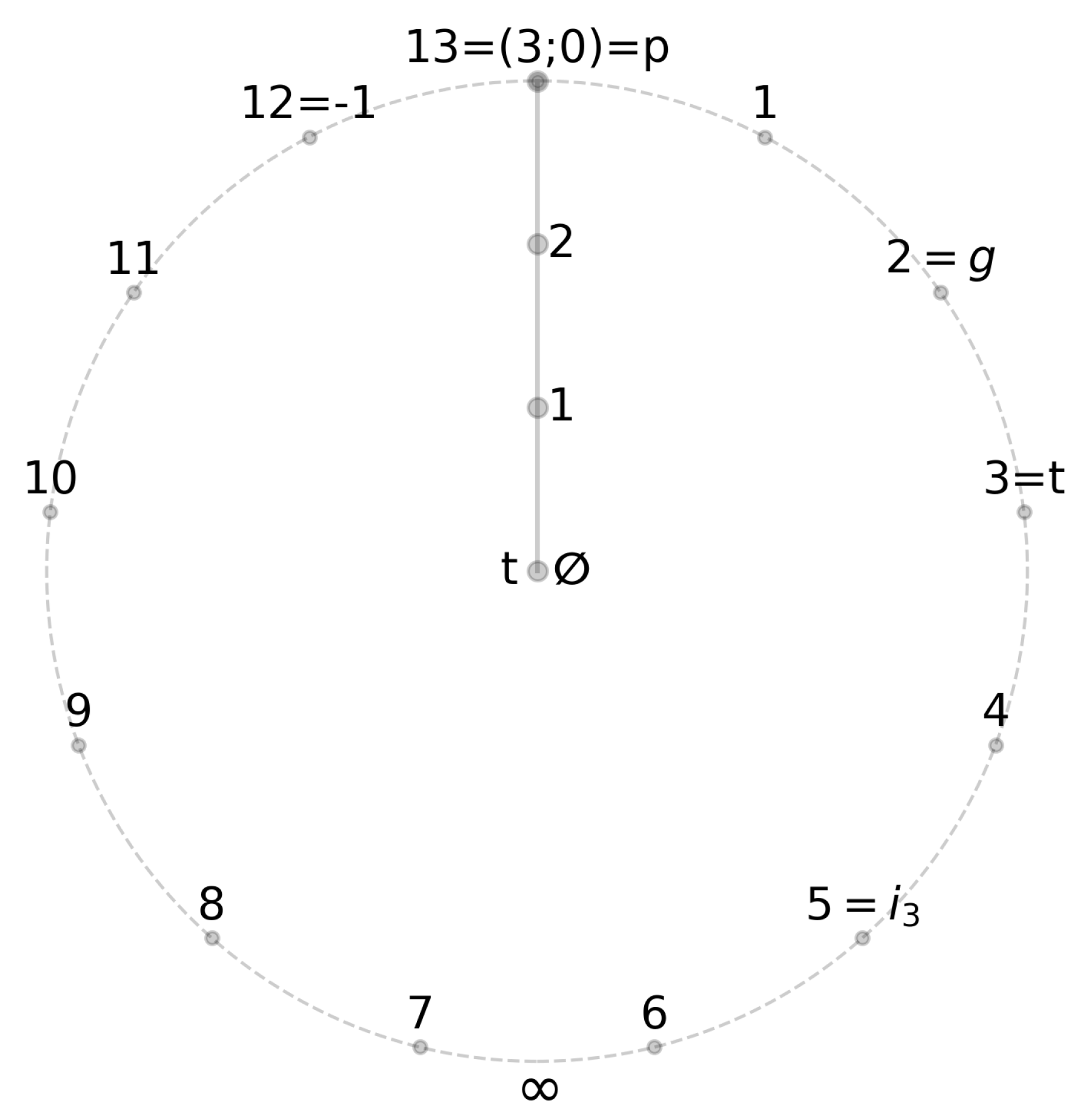
To exemplify, let us now consider the concrete example of and the corresponding finite framed field . We can identify the value of the imaginary unit . The corresponding visual representation of the finite field is shown in Figure 9. The figure shows the state space of the finite field as a circle on a 2D plane, with the major structural elements , as well as ∞ indicated. The antipodal point ∞ is located at the South Pole of the pseudo-sphere, which is the farthest point from the observer at 0.
5.2. Finite Langlands Program
In the conventional Langlands philosophy one relates two vast worlds: on the one hand the (infinite) Galois representations of a global field, and on the other the automorphic representations of a reductive group over that field [31,32]. If one accepts that only finite rings can exist, then every “infinite” Galois group must be replaced by its finite quotient
and every automorphic representation must likewise factor through a finite group of points
for some level . In this finite-Langlands perspective all objects—Galois data and automorphic forms—are built from the same finite base ring , and the conjectural correspondence becomes a bijection between
From the function-field side one already has a prototype: Drinfeld and Lafforgue proved a global Langlands correspondence for over , where is a finite field, and automorphic forms live on [33,34]. There, both Galois representations and automorphic sheaves are intrinsically finite objects—perverse sheaves on moduli stacks over and ℓ-adic representations of . This suggests that a genuinely finite-universe version of the Langlands program would reorganise every classical component (Hecke operators, L-functions, trace formulas) into purely combinatorial operations on -modules and finite group characters.
In summary, if one accepts that is the only ontologically primitive object, then the Langlands correspondence reduces to an equivalence of categories between -linear Galois modules and -linear automorphic modules. All “infinite” phenomena (analytic continuation, spectral decompositions) become emergent from the finiteness of through limiting processes within finite-dimensional -vector spaces. Such a viewpoint collapses the traditional dichotomy and recasts Langlands duality as a statement about different frames of reference on a single finite ring.
6. Conclusions
The primary objective of this work has been to devise an algebraic framework that (1) does not contradict our conventional arithmetic and geometric intuitions, (2) enables all practical applications of modern mathematics, and (3) completely disposes of the ontological need for actual infinity. We have shown that by interpreting addition, multiplication and exponentiation as internal symmetries of a finite framed field , one can reconstruct signed integers, pseudo-rationals, pseudo-reals and pseudo-complex numbers in a way that matches classical behaviour up to any desired precision, without ever invoking an infinite set. This construction preserves the familiar algebraic laws and analytic operations that underpin standard number systems, ensuring full compatibility with intuition and established mathematical practice.
Moreover, the resultant FRC framework supports the full spectrum of modern mathematical techniques—solving polynomial equations, performing limit-like approximations via dense pseudo-rationals, and modelling continuous symmetries through -Lie-group approximations—while entirely replacing classical infinities with context-dependent finite representations. In doing so, it provides exact algebraic analogues for roots, exponentials and trigonometric relationships, and offers a discrete yet arbitrarily precise scaffold for differential-geometric and analytic constructions. By eliminating any ontological reliance on actual infinity, this framework retains the power and flexibility of conventional mathematics in a fully finitary setting, while also offering an avenue towards the resolution of classical paradoxes of logic and set theory imposed by the infinitude conjecture. The resulting structure is not merely a mathematical curiosity; it is a coherent and physically grounded alternative to standard formalism, suitable for the description of discrete, informationally finite physical systems.
Looking forward, extending our framework to composite moduli, and exploring the implications for the analysis of dynamic physical systems, will further strengthen and broaden its applicability. We anticipate that this relational, finite approach will serve as both a conceptually coherent foundation and a practical computational paradigm across mathematics, physics, formal logic and computer science.
Notation Glossary
- Foundational parameter.
- Prime number that is the order of the finite field.
- Finite field of prime cardinality
- The class of signed pseudo-integers over the finite field (Definition 5)
- The class of pseudo-rational numbers over the finite field (Definition 6)
- The class of truncated pseudo-rational numbers over the finite field with a bounded scale H (Definition 7)
- The class of pseudo-real numbers over the finite field (Definition 7)
- The class of pseudo-complex numbers over the finite field (Definition 8)
Author disclosure. Portions of this work were reviewed with the assistance of ChatGPT (OpenAI, model o3, April-June 2025) to verify theorem statements, suggest proof refinements, and streamline language and formatting. All formal arguments and final text were subsequently checked and approved by the authors, who accept full responsibility for the content.
References
- Lane, S.M. Categories for the Working Mathematician; Springer, 1998.
- Einstein, A. On the Electrodynamics of Moving Bodies. Annalen der Physik 1905, 17, 891–921. [Google Scholar] [CrossRef]
- Noether, E. Invariante Variationsprobleme. Nachrichten von der Gesellschaft der Wissenschaften zu Göttingen, Mathematisch-Physikalische Klasse.
- Akhtman, Y. Existence, Complexity and Truth in a Finite Universe. Preprints 2025. [Google Scholar]
- Smolin, L. Time Reborn: From the Crisis in Physics to the Future of the Universe; Houghton Mifflin Harcourt, 2013.
- Smolin, L. The Trouble with Physics: The Rise of String Theory, the Fall of a Science, and What Comes Next; Houghton Mifflin Harcourt, 2006.
- Lev, F. Finite Mathematics as the Foundation of Classical Mathematics and Quantum Theory; Springer International Publishing, 2020. [CrossRef]
- D’Ariano, G.M. Physics Without Physics: The Power of Information-Theoretical Principles. International Journal of Theoretical Physics 2017, 56, 97–128. [Google Scholar] [CrossRef]
- Benci, V.; Nasso, M.D. Numerosities of Labelled Sets: A New Way of Counting. Advances in Mathematics 2003, 173, 50–67. [Google Scholar] [CrossRef]
- Benci, V.; Nasso, M.D. A Theory of Ultrafinitism. Notre Dame Journal of Formal Logic 2011, 52, 229–247. [Google Scholar]
- Yessenin-Volpin, A.S. The Ultra-Intuitionistic Criticism and the Antitraditional Program for Foundations of Mathematics. Proceedings of the International Congress of Mathematicians.
- Parikh, R.J. Existence and Feasibility in Arithmetic. Journal of Symbolic Logic 1971, 36, 494–508. [Google Scholar] [CrossRef]
- Sazonov, V.Y. On Feasible Numbers. Logic and Computational Complexity.
- Avron, A. The Semantics and Proof Theory of Linear Logic. Theoretical Computer Science 2001, 294, 3–67. [Google Scholar] [CrossRef]
- Brouwer, L.E.J. On the Foundations of Mathematics; Springer, 1927.
- Weyl, H. Philosophy of Mathematics and Natural Science; Princeton University Press, 1949.
- Chaitin, G. Thinking about Gödel and Turing: Essays on Complexity, 1970-2007. World Scientific 2007. [Google Scholar]
- Lloyd, S. Ultimate Physical Limits to Computation; Nature, 2000.
- Akhtman, Y. Geometry and Constants in Finite Ring Continuum. Preprints 2025. [Google Scholar]
- Akhtman, Y. Finite Ring Continuum at Composite Cardinalities. Preprints 2025. [Google Scholar]
- Burton, D.M. Elementary Number Theory, 7th ed.; McGraw-Hill, 2010.
- Dummit, D.S.; Foote, R.M. Abstract Algebra, 3rd ed.; John Wiley & Sons, 2004.
- Knuth, D.E. The Art of Computer Programming, Volume 1: Fundamental Algorithms, 3rd ed.; Addison-Wesley, 1997.
- Serre, J.P. Local Fields; Vol. 67, Graduate Texts in Mathematics, Springer: New York, 1979. [Google Scholar]
- Turing, A.M. On Computable Numbers, with an Application to the Entscheidungsproblem. Proceedings of the London Mathematical Society 1936, 42, 230–265. [Google Scholar]
- Lamé, G. Mémoire sur la résolution des équations numériques. Comptes Rendus de l’Académie des Sciences 1844, 19, 867–872. [Google Scholar]
- Rudin, W. Principles of Mathematical Analysis, 3rd ed.; McGraw-Hill: New York, 1976. [Google Scholar]
- Wilson, K.G. Renormalization group and critical phenomena. I. Renormalization group and the Kadanoff scaling picture. Physical Review B 1971, 4, 3174–3183. [Google Scholar] [CrossRef]
- Cardy, J. Scaling and renormalization in statistical physics; Cambridge University Press, 1996.
- Barwise, J.; Perry, J. Situations and Attitudes; MIT Press, 1985.
- Langlands, R.P. Problems in the Theory of Automorphic Forms; Springer-Verlag, 1970.
- Borel, A. Automorphic Forms on Reductive Groups; Springer-Verlag, 1979.
- Drinfeld, V.G. Elliptic modules. Mathematics of the USSR-Sbornik 1974, 23, 561–592. [Google Scholar] [CrossRef]
- Lafforgue, L. Chtoucas de Drinfeld et correspondance de Langlands. Inventiones mathematicae 2002, 147, 1–241. [Google Scholar] [CrossRef]
| 1 | The detailed interpretation of the role of is provided in [19]. Here we leave it as a fixed parameter that determines the field cardinality . |
Figure 1.
Progression of results from the foundational Algebra manuscript to subsequent papers on Geometry and Composition.
Figure 1.
Progression of results from the foundational Algebra manuscript to subsequent papers on Geometry and Composition.
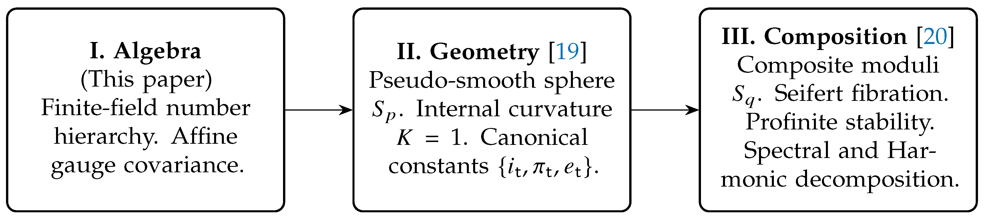
Figure 2.
Diagram of a finite field , typically visualized as a circle on a 2D plane that illustrates its periodicity and rotational symmetry under the arithmetic operation of addition. The radial axis represents the corresponding foundational parameter .
Figure 2.
Diagram of a finite field , typically visualized as a circle on a 2D plane that illustrates its periodicity and rotational symmetry under the arithmetic operation of addition. The radial axis represents the corresponding foundational parameter .
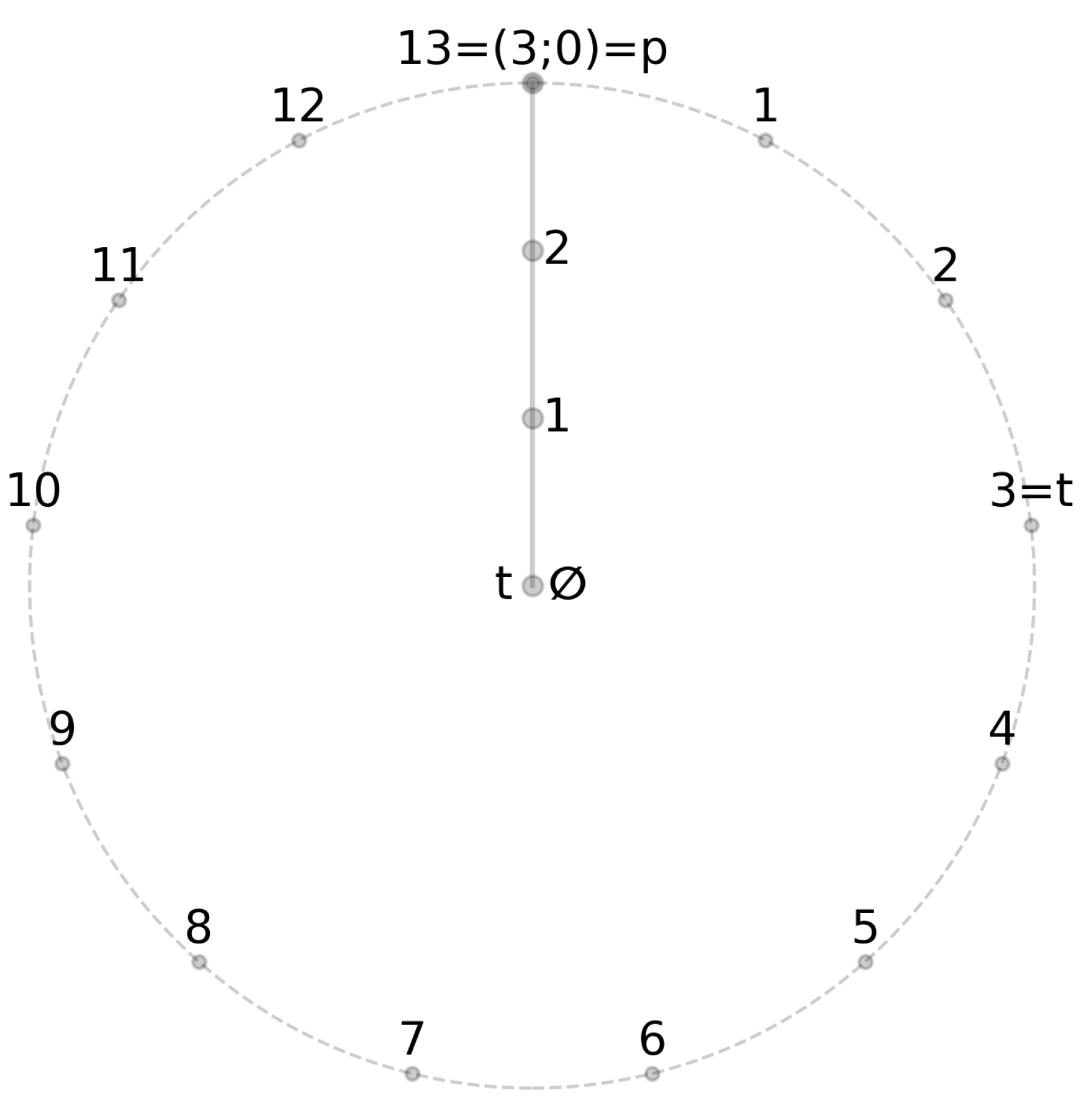
Figure 3.
State diagram for framed finite field as a 2D spheroid in 4D symmetry space combining the additive symmetry along the meridians , as well as multiplicative symmetry along the latitudes for multiplicative generator .
Figure 3.
State diagram for framed finite field as a 2D spheroid in 4D symmetry space combining the additive symmetry along the meridians , as well as multiplicative symmetry along the latitudes for multiplicative generator .
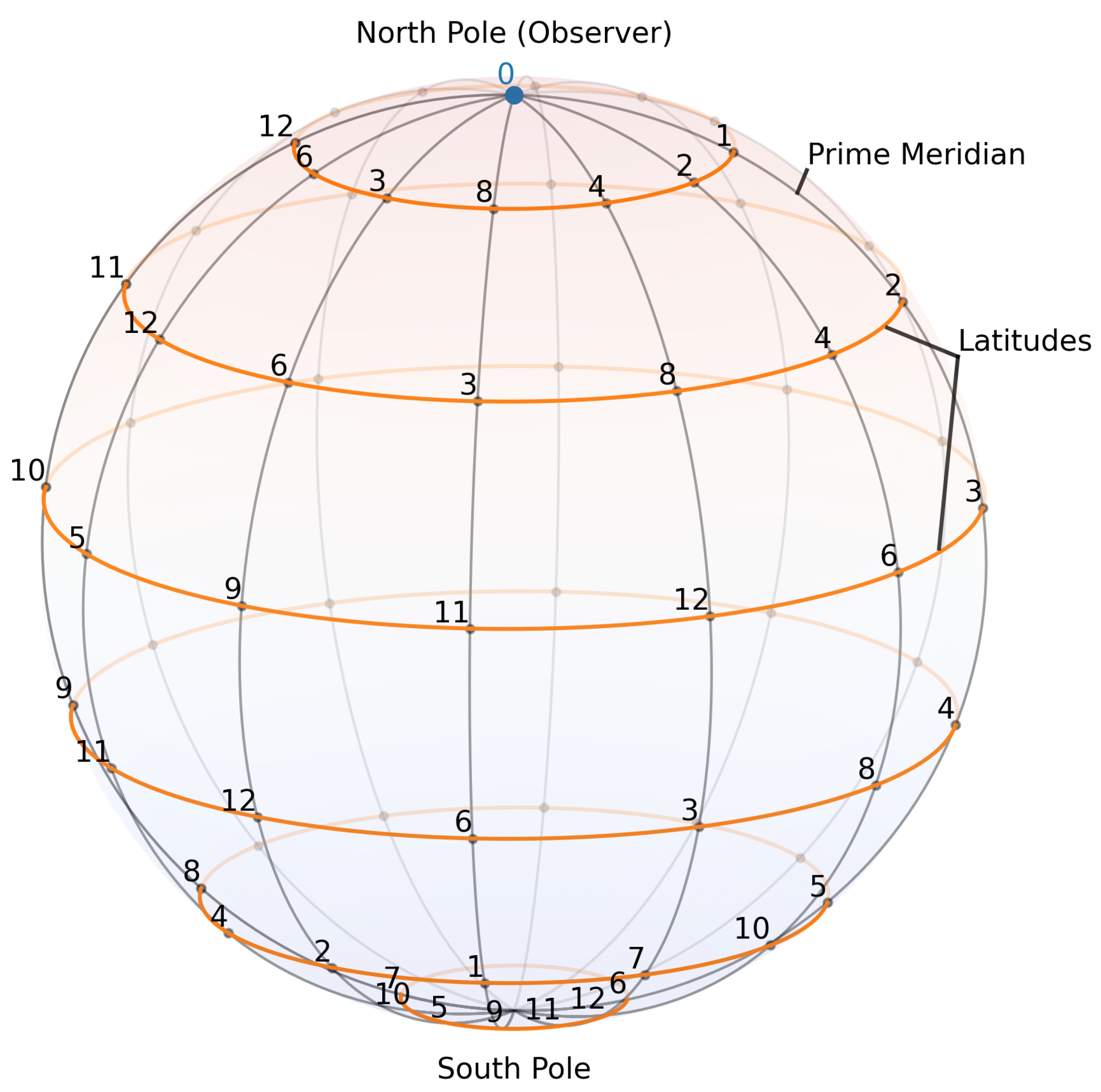
Figure 4.
Class of signed pseudo-integers over the finite framed field . Black labels indicate the newly defined signed pseudo-integers , while the purple labels represent the corresponding elements . The unlabelled gray dots indicate the off-axis elements of observed from the top of the 2D spheroid described in Section 3 and depicted in Figure 3.
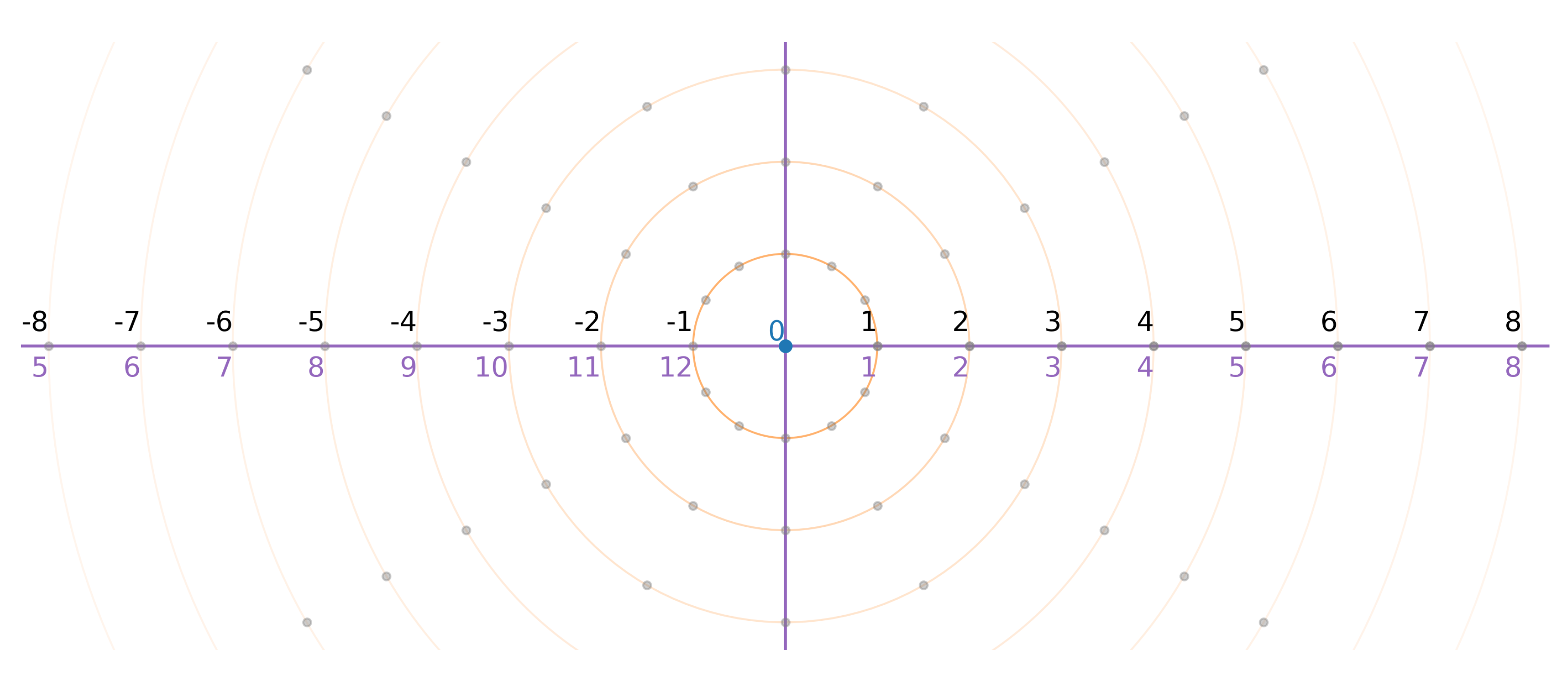
Figure 5.
Few examples of rational numbers in a finite framed field . Note the pseudo-rational numbers and that represent the exact same element .
Figure 5.
Few examples of rational numbers in a finite framed field . Note the pseudo-rational numbers and that represent the exact same element .
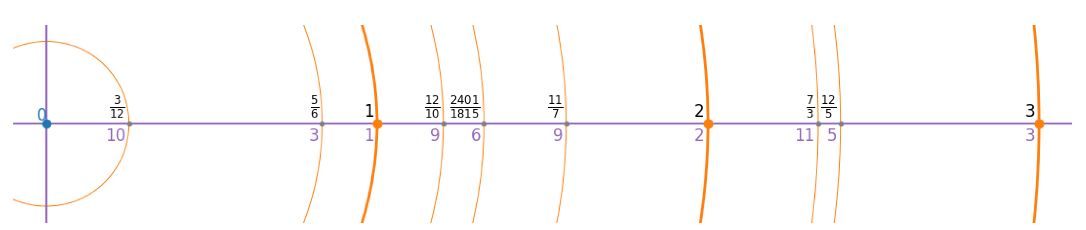
Figure 6.
Uniform grid of rational numbers of the form with step size . Here, we have , and . Black labels indicate the pseudo-rational numbers , while the purple labels represent the corresponding finite field elements . The blue line indicates the periodicity of the finite field.
Figure 6.
Uniform grid of rational numbers of the form with step size . Here, we have , and . Black labels indicate the pseudo-rational numbers , while the purple labels represent the corresponding finite field elements . The blue line indicates the periodicity of the finite field.
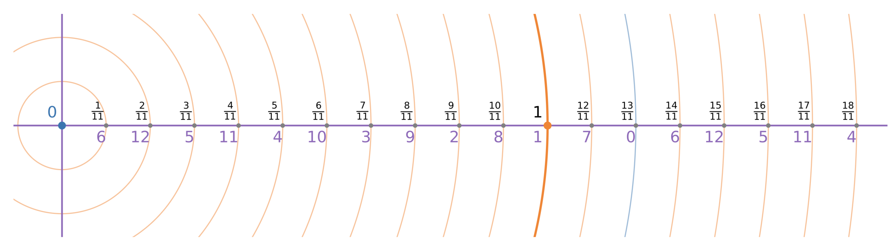
Figure 7.
Scale-periodicity for and generator . After zoom steps the grid of pseudo-rationals repeats exactly. The red arrows visualize the identification between corresponding points along pseudo-real axis and across zoom steps. Black labels indicate the pseudo-rational points , while the purple labels denote the corresponding finite field elements . The grid is invariant under multiplication by , demonstrating the periodicity of the zoom operation.
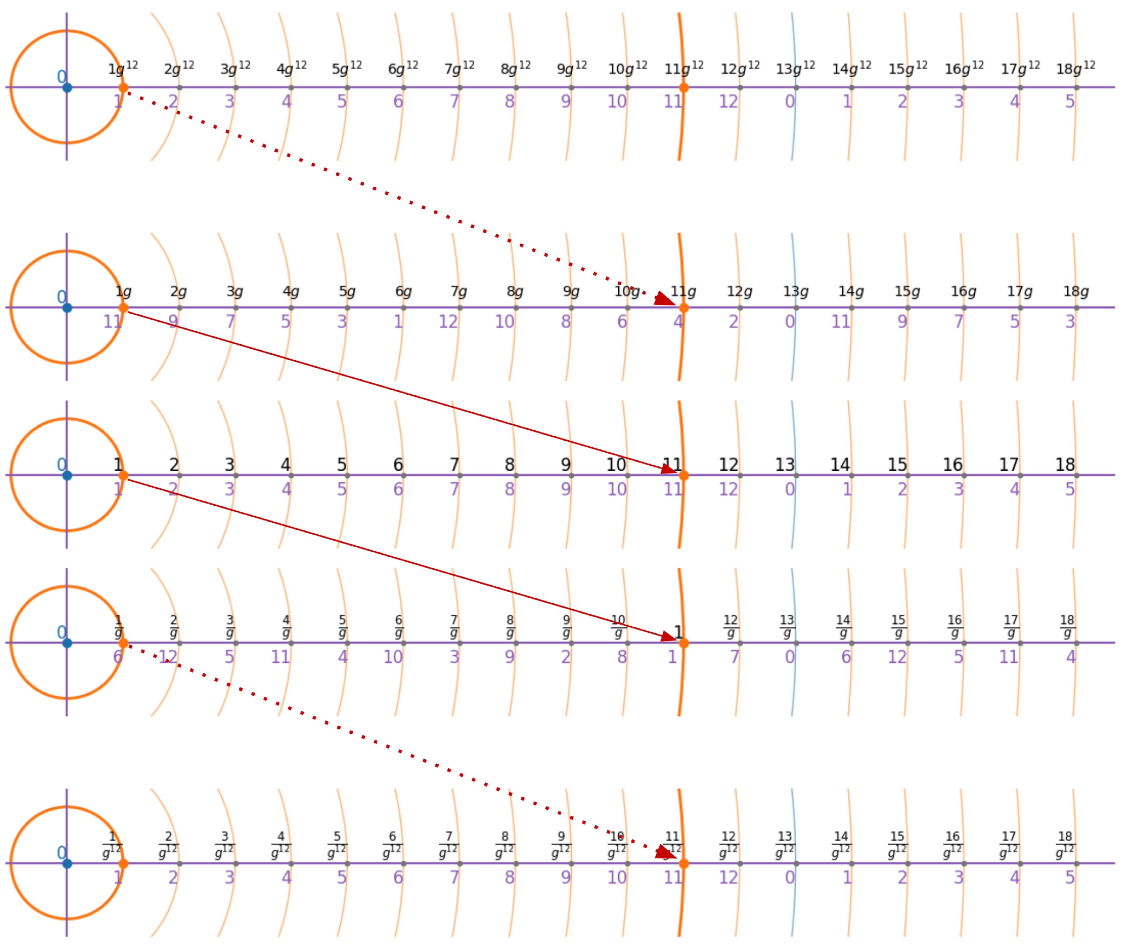
Figure 8.
Pseudo-complex numbers plane in a finite framed field . Horizontal axis represents the pseudo-reals on the prime meridian and the vertical axis represents the imaginary numbers indicated by their respective red labels. The corresponding elements are depicted in purple. The blue line indicates the periodicity of the finite field.
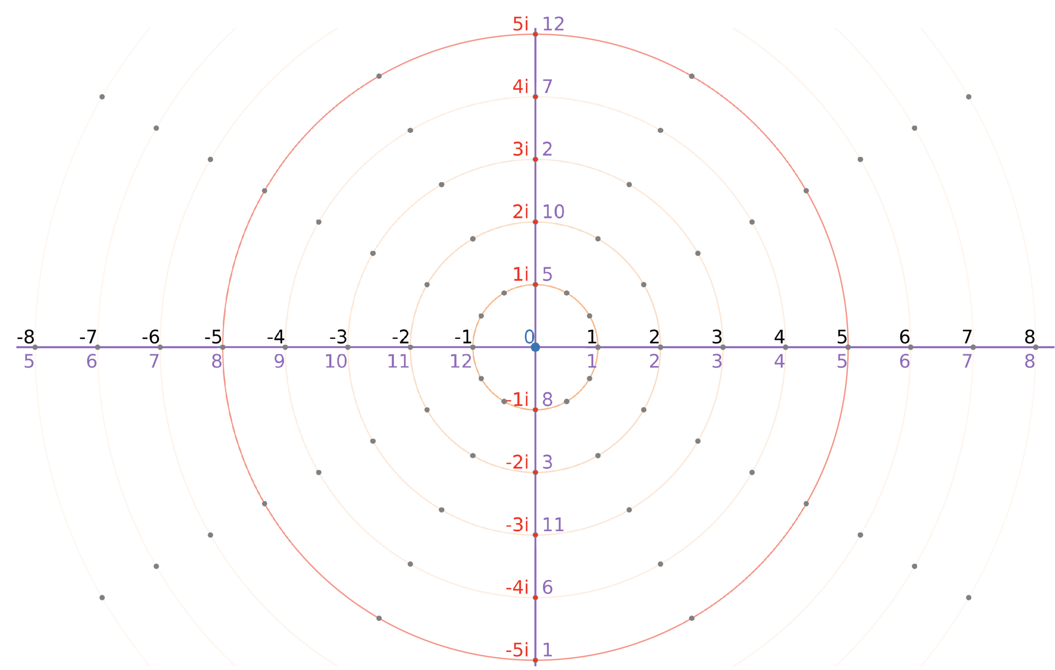
Figure 9.
State space of a finite framed field , visualized as a circle on a 2D plane with the major structural elements , as well as ∞ indicated.
Figure 9.
State space of a finite framed field , visualized as a circle on a 2D plane with the major structural elements , as well as ∞ indicated.
Disclaimer/Publisher’s Note: The statements, opinions and data contained in all publications are solely those of the individual author(s) and contributor(s) and not of MDPI and/or the editor(s). MDPI and/or the editor(s) disclaim responsibility for any injury to people or property resulting from any ideas, methods, instructions or products referred to in the content. |
© 2025 by the authors. Licensee MDPI, Basel, Switzerland. This article is an open access article distributed under the terms and conditions of the Creative Commons Attribution (CC BY) license (http://creativecommons.org/licenses/by/4.0/).
Copyright: This open access article is published under a Creative Commons CC BY 4.0 license, which permit the free download, distribution, and reuse, provided that the author and preprint are cited in any reuse.


