
Submitted:
26 May 2025
Posted:
27 May 2025
You are already at the latest version
Abstract
This study investigates shear cutting of high-strength steel sheets, a process known to negatively impact the forming and fatigue properties of the material. The localized deformation near the cut edges imposes sheared edge damage, especially in advanced high-strength steels where severe shear deformation occurs in the very vicinity of the cut edge. In this work, an extensive experimental investigation was carried out on punched holes of thin sheets, using light optical microscopy and metallographic techniques for sheared edge damage assessment. These methods provided detailed insights into the sheared edge damage and offer a thorough understanding of the deformation behavior in the shear-affected zone. Advanced engineering cut edge investigation methods have been developed based on 2D and 3D stereo light microscopy for non-destructive panoramic cut edge parameters and cut edge profiles determination along cut hole circumference. Such methods provide an efficient evaluation instrument for challenging close cut holes, with the possibility of industrial in-line monitoring and machine learning applications towards Industry4.0 implementation. Additionally, the study compares grain shear angle measurement and Vickers indentation for deformation assessment of the cut edge. It concludes that grain shear angle offers higher resolution and is postulated as a relevant parameter to assess the sheared edge zone. The findings contribute to a deeper understanding of sheared edge damage and improve evaluation methods, potentially enhancing the use of high-strength steels in automotive and safety-critical applications.
Keywords:
Shear cutting
; Shear affected zone
; Sheared edge damage
; Grain shear angle
; non-destructive testing
; Advanced high strength steel
1. Introduction
Shear cutting remains the most common cutting technique in the cold sheet forming process, due to automation possibilities and cost-efficiency. This technique involves a shearing process where the sheet metal is separated by a moving punch, pushing the workpiece against the fixed die. This process typically results in the formation of a cut edge with a characteristic profile, consisting of the rollover formation, the burnish zone, the fracture zone, and the burr formation, as seen in Figure 1 (a). Figure 1 (b) shows the distinction between primary and secondary burnish and fracture, features that might appear at low cutting clearances.
While shear cutting offers efficiency and precision, the nature of the operation inevitably causes localized deformation and damage to the material, which can manifest as burrs, micro-cracks, and strain hardening near the cut edge [1]. This region, often referred to as the Shear Affected Zone (SAZ), is known for affecting the formability of sheared parts and triggering edge cracking, especially for Advanced High Strength Steels (AHSS) [2]. This has been experimentally shown for both close cuts [3] and open cuts [4], varying cutting clearance and material grade [5] and with varying punch tool design [6]. The sheared edge damage is also known to affect the fatigue properties of high strength sheets since the cutting process induces microcracks and notches [7,8,9] and residual stresses to the cut edge [10,11]. Sheared edge damage is also a factor in hydrogen embrittlement of AHSS [12,13]. Factors influencing the characteristics of the SAZ include the material mechanical properties and cutting conditions (such as cutting clearance, cutting speed and tool wear) [14]. For instance, AHSS grades with ultimate tensile strength (UTS) of 1000 MPa and above, now increasingly used in lightweight construction and safety-critical applications, are particularly susceptible to localized sheared edge damage due to their higher strength and reduced ductility compared to lower strength conventional AHSS sheets. As a result, understanding and controlling the residual state of the SAZ, introduced by shear cutting, is important for ensuring product reliability and optimizing performance during the manufacturing process.
Traditionally, sheared edge damage investigation has been performed at different magnification levels, starting from naked eye observation, to microscopic investigation and using metallographic techniques for detailed analysis. Figure 2 shows conventional cut edge inspection techniques and presents typical appearance of secondary burnish in close cut hole edge, as well as burr and fracture surface roughness. Figure 3 shows the open cut secondary burnish formation in different proportion, from little to strongly manifested secondary burnish merging with primary burnish. Some irregular burr and rough cut edge fracture surface are also displayed.
Detailed investigations of sheared edge damage are conventionally performed using destructive techniques, such as cross-sectional analysis through metallography and microhardness tests. These methods provide valuable insights into the extent of SAZ damage, allowing quantification of the degree of deformation and identify defects like cracks, voids, or brittle phases. However, the destructive nature of these methods limits their applicability, especially in cases where circumferential heterogeneity and spatial variations in sheared edge damage need to be assessed. Such circumferential heterogeneities typically appear in punched sheet holes in industrial forming lines and reduce the stretch-flangeability of the edge [15], due to unavoidable tool wear or tool misalignment during part production. In contrast, the use non-destructive cut edge assessment methods does allow for repeated use of the shear cutting specimens and are required for in-line measurements. In this work, the main focus is laid on conventional readily and widely available non-destructive testing methods using light optical microscopy (LOM) which is part of the standard equipment in industrial laboratory environments. Therefore, expensive, time consuming and punctual detailed non-destructive methods such as scanning electron microscopy (SEM) or electron backscatter diffraction (EBSD) are disregarded, although their use in laboratory SAZ damage identification is well proven [16,17,18].
This study investigates the sheared edge damage in a 1.5 mm complex-phase advanced high-strength steel (AHSS) with UTS MPa, which is characterized by highly localized shear deformation and a narrow shear-affected zone (SAZ). Such localization challenges the assessment of edge quality and its influence on subsequent forming and fatigue performance. The experimental work presented in this article is based on hole punching using varying process parameters, where the resulting damage was analyzed across macro, meso, and micro length scales. Conventional SAZ characterization methods, including Vickers hardness (DIN ISO 6507) [19], which is frequently used in conventional cutting [20,21], two-stage shear cutting [22], and post-cutting fatigue studies [10], and grain shear angle measurements [12,23,24,25], are evaluated for their suitability in large-sample investigations. In addition, the study explores the use of 2D panoramic and 3D profile microscopy as efficient, non-destructive techniques for detailed cut edge assessment, particularly for small, close-cut geometries. The overall objective is to improve the reliability of SAZ characterization and propose practical, scalable methods to address the heterogeneous edges typical of high-strength steels. The methods developed in this work make use of cost-effective microscopy instruments with minimal image processing, providing both research and industry with valuable tools to enhance shear cutting processes and improve the formability and fatigue resistance of AHSS components.
2. Materials and Methods
In the present article, the 1.5mm CR700Y980T-CH automotive sheet steel by voestalpine Stahl GmbH was investigated in the cold rolled pickled and continuously annealed condition. This grade will be referred in the following as CP1000HD. This is a cold rolled complex phase steel with high ductility and an ultimate tensile strength of 1000 MPa. This material is common in automotive applications, such as crash management systems and structural components. The CP1000HD grade has a fine grained microstructure consisting of homogeneous bainite, martensite and retained austenite. The mechanical tensile properties of the CP1000HD grade are shown in Table 1.
2.1. Sheet Punching
Sheet punching is a shear cutting process commonly applied in the sheet forming industry prior to hole collaring operations and for creation of bolt joints. This process produces a hole in the sheet using a fixed die and a moving punch in a closed cut condition according to the schematic image of Figure 4.
The most significant process parameter of the hole punching process is the cutting clearance (Cl), which denotes the horizontal space between the punch and the die. Cutting clearance is expressed as a percentage according to Equation (1), where and denotes the die and punch radius and is the blank thickness.
The sheet punching experiments conducted in this work were performed according to the ISO16630 HET standard procedure [26], which describes a testing method used for evaluating the stretch-flangeability of sheet metals. The experiments were conducted for cutting clearances ranging from 5% to 40% using a servo-hydraulic machine with a ISO16630 dedicated hole punching tool with 150 kN maximum load. The total press cylinder force was recorded with a calibrated 200 kN strain gauge load cell and the punch displacement was measured with a 100 mm Linear Variable Differential Transformer (LVDT) inductive displacement sensor. A total force of 5 to 15 kN was required for the blank holder spring device before punching. The punching depth was adjusted so that the bottom dead center corresponds exactly to the full material thickness. The punching piston speed, with a range of 0.05-55 mm/s, was set to 0.05 mm/s, corresponding to quasi-static loading conditions. The testing procedure described in the ISO standard is performed in quasi-static conditions, thus reducing the dynamic processing effects such as strain-rate dependency and adiabatic heating of the material. Such effects are otherwise common in industrial process, but in the present study are they disregarded for a more clear discerning of the material deformation behavior.
The punching of a 10 mm diameter ISO16630 hole in the center of a 100x100 mm sheet sample was made with a dedicated 4 columns tool (Figure 4 (a)) with tight coaxiality specifications (±5 µm) between upper and lower tool as well as high fitting accuracy for punch and die inserts (±5 µm). This allowed for an accurate (±1%) cutting clearance compliance around the cut hole perimeter. The punching tools (punch and die) were made of high performance tool material with titanium carbonitride coating. Sharp tools were used with a circular cutting edge of estimately 30 µm radii. All geometric cutting parameters are presented in Table 2.
The effect of non-coaxiality on the ISO16630 test was previously reported as one of the main causes of the well-documented results scatter from this test [27]. Due to this, the coaxiality of the ISO16630 dedicated hole punching tool used in the present work was controlled by interrupted punching of a paper sheet. Figure 5 shows the results from paper punching where a slight unevenness in punch intrusion was detected. This caused some circumferential variation of the cutting clearance and consequently, the cut edge morphology, to be further discussed in Section 4.
2.2. Cut Edge Investigation and Shear Affected Zone
Following the hole punching experiments, the cut edges were investigated and the distribution of cut edge parameters was determined. The cut edge parameters, schematically shown in Figure 1, consist of rollover formation, burnish surfaces, fracture surfaces and possible burr formation. Cut edge investigations are challenging since local formation of cut edge parameters may vary within narrow ranges of the hole circumference and through the blank thickness. Naked eye evaluation with 2-3x magnifying glass is largely insufficient at best suitable for a quick evaluation of burnish-to-fracture ratio or burr presence evaluation.
A digital portable USB microscope with 50x magnification has proved to be much more useful for daily laboratory qualitative investigation of industrial components or testing samples with cut edge issues, as shown in Figure 6 (a). Indirect conclusions can be drawn from cut edge condition regarding cutting tool wear of punch and die as well as coaxiality and clearance of cutting tools. Quantitative cut edge investigations require however some more advanced methodology. A classic method would be with metallographic cross sections shown in Figure 6 (b), which is particularly useful for determining the local clearance, the fracture angle or burr presence. This is however a destructive and time-consuming testing method, which delivers a precise cut edge information but only for a very specific location.
In this work, a focus has been laid on advanced non-destructive optical methods for cut edge investigations in close-cut hole conditions. Traditionally, cut edge characterization relies on destructive techniques such as metallographic cross-sections and microhardness indentation, typically using Vickers hardness testing. While these methods provide valuable information on local work hardening and deformation, they are limited to single cross-sections, are time-consuming, and cannot capture variations along the full hole perimeter. To overcome these limitations, two optical methods have been developed. The first, referred to as EISYS (Edge Inspection System), provides a 360° panoramic 2D front view of the entire hole perimeter, enabling fast and comprehensive mapping of cut edge features. The second method utilizes a high-magnification 3D stereo microscope to reconstruct detailed 3D edge profiles at selected positions along the hole circumference. In addition to these optical techniques, this study introduces grain shear angle measurement as a relatively new and physically meaningful way to characterize SAZ deformation. This approach offers higher spatial resolution and better captures localized shear deformation compared to conventional hardness-based methods, providing a valuable extension to established cut edge assessment techniques.
2.2.1. 2D Optical EISYS Methodology
A cut edge inspection tool designed for delivering a panoramic view of the cut edge surface was used for the characterization of 10 mm diameter holes prepared under different punching conditions on 100x100 mm ISO16630 samples [28]. The cut edge parameters were determined with the optical device shown in Figure 7 and Figure 8. A preliminary manual centering device was used with the specimen in burr down configuration (Figure 7 (a) and (b)). The whole clamping tool cassette was then transferred to the optical device and 360° rotated in 2° intervals along hole perimeter (Figure 7 (c) and (d)). The sample rotation was accurately centered around a 5x5mm 45° reflecting fixed mirror, enabling a frontal orthogonal projected view on the hole cut edge and allowing accordingly for an accurate quantitative panoramic cut edge parameter analysis for material thickness up to around 3-3.5 mm. Each time pictures were generated with three lightning configurations as shown in Figure 8 (b)-(d) (coaxial, oblique left, oblique right). Red backlight for upper rollover side and green backlight on lower burr side also help identifying the cut edge boundaries. The local thickness was also measured manually around hole location. After 360° stitching of all pictures together, the developed cut edge parameters profiles for rollover, burnish, fracture and burr height were determined via image analysis according to Figure 9.
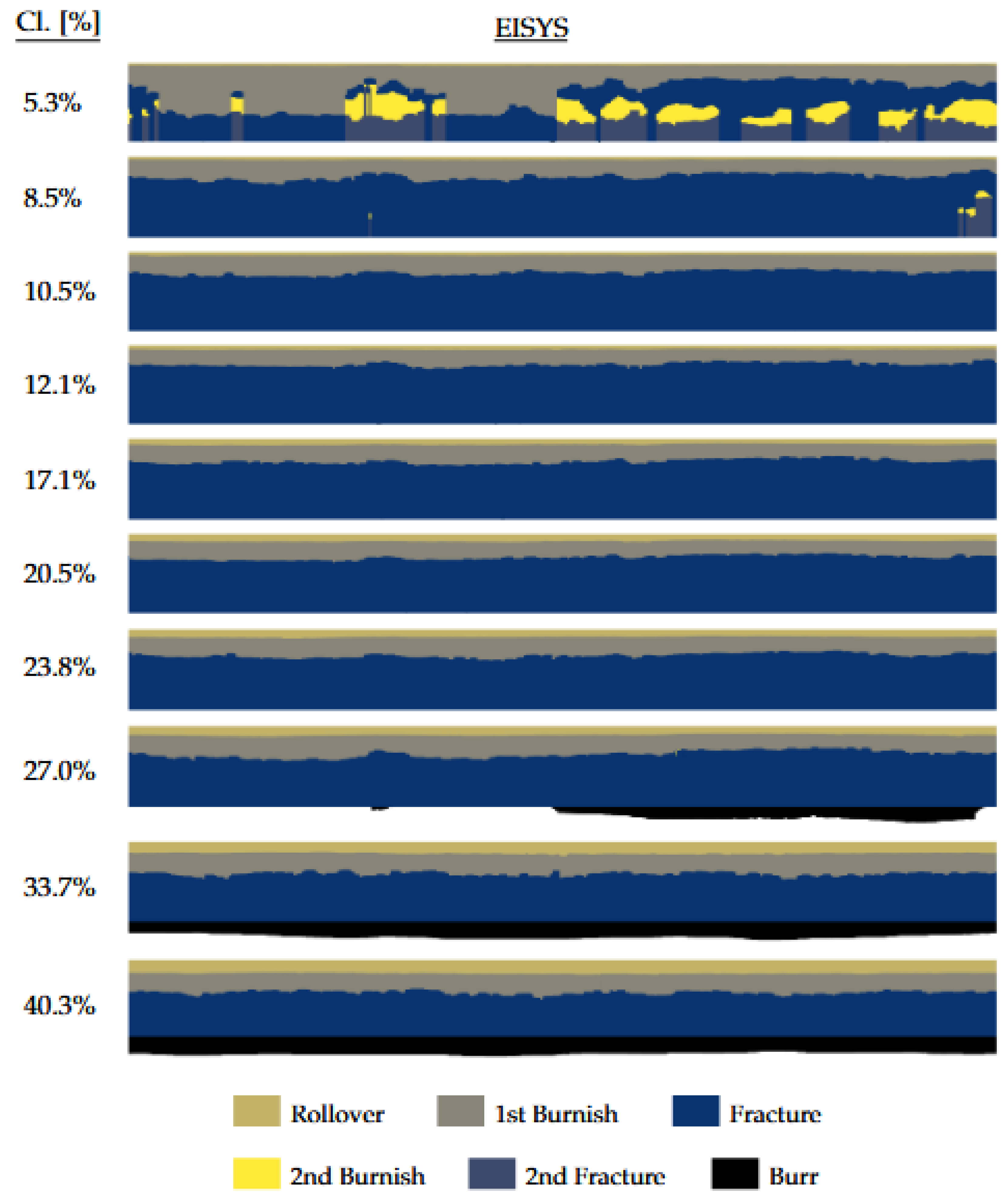
Figure 9 (a)-(c) shows the raw panoramic images of the punched hole using 27% cutting clearance and the identified cut edge parameters. Figure 9 (d) delivers the digitalized distribution of the cut edge parameters. Additionally, Figure 9 (e) gives a bar chart of the average cut edge parameter distribution over the blank thickness and the error bars show the circumferential variation (standard deviation) of each cut edge parameters. The EISYS procedure was performed for all cutting clearances presented in Table 2 and the reconstructed panoramic images of the cut edges, plotting the relative proportion of cut edge parameters, are shown in Appendix A.
2.2.2. 3D Stereo Optical Cut Edge Methodology
A Keyence stereo 3D microscope (VHX-7000) device has been used to measure the full 3D cut edge profiles of punched edges around the hole perimeter in 90° steps with regard to rolling direction (0°, 180° cross section along rolling direction, 90, 270° cross section transverse to rolling direction). A scan was performed with the Keyence microscope in Z-direction through the focal range of a sample in order to build a fully-focused image with a large working distance (depth of field ≈25 mm), similar to already proven technique [29,30]. The pre-selected X-Y area was then scanned delivering a 2D/3D stitched image, as shown in Figure 10 (a). Virtual 3D profiles cross sections shown in Figure 11 (a)-(c) were then generated from recorded images. While rollover and burr side information were obtained directly from horizontally lying sample (Figure 11 (a),(c)), the front view (Figure 11 (b)) of the actual cut edge 90° to burnish was obtained by a mirror technique. As for the EISYS 2D technique, a small free moving 5x5 mm 45° prismatic glass mirror was introduced manually in front of cut edge reflecting the cut edge vertical image into a flat image into the objective (Figure 10 (b)-(d)). In this way, a 3D cut edge picture from a mirror view can still be processed in the 3D stereo microscope, which was particularly advantageous for cut hole edge investigations. Such a mirror reflection technique allows a non-destructive analysis of around 4 mm wide local cut edge sections at any location along hole edge.
The cut edge profiles were then built by combining the individual top, down and front view virtual profiles with simple translation/rotation image analysis operations as displayed in Figure 11 (d). With following geometric conditions the whole cut edge profile can be reconstructed from individual rollover, front view mirror and burr profiles: blank thickness being accurately measured, upper and lower edges horizontally assumed in bulk material region far away from cut edge and a vertical orthogonal cut along primary burnish-punch axis for X=0. The 3D stereo optical cut edge methodology presented in this work requires the combination of only three recorded images, thereby minimizing image post-processing and ensuring low computational cost. This makes the advanced Keyence stereo 3D microscope mirror technique ideal for rapid cut edge measurements, utilizing an affordable and minimal equipment setup.
Some advantages of such advanced experimental optical technique in comparison to traditional metallographic cross section are the broader general overview of cut edge shape, as well as the freedom of virtual cuts which can be repeated without destruction of the cut edge samples as in metallographic sections. From those virtual 3D cut edge profiles the evolution and scattering of cut edge conditions versus cutting process parameters along the hole perimeter can be determined at whatever location needed. The optical resolution reached around 1-2 µm at 400x magnification, which was high enough for accurate 3D cut edge parameters determination, especially useful for local cutting clearance, horizontal rollover, fracture angle or burr width parameters, which were not delivered by the 2D front view panoramic EISYS device. Both non-destructive optical techniques from 2D EISYS panoramic views and 3D stereo microscope profiles complement each other. More time consuming specific metallographic cross sections were therefore only mandatory for more in depth microstructure and grain shear angle analysis from etched cut edge cross sections.
With the experimental cut edge profiles, the fracture angles were measured at positions located at , , and around the hole circumference for each cutting clearance. In this work, the fracture angle was determined between a best fit tangential line in fracture zone and the vertical burnish surface axis [7]. Figure 12 shows how the fracture angle was defined for both (a) no-burr and (b) burr conditions, whereas (c) shows the two fracture angles and associated with secondary burnish formation.
2.2.3. Metallographic Cut Edge Investigation - Vickers Hardness Measurement
Local shear deformation of the SAZ was evaluated using Vickers micro hardness tests in accordance with the ISO 6507-1 standard [19] on metallographic cross sections of cut edges for a separate section per cutting clearance, aligned with the rolling direction. Given the near isotropic behavior of the material, time consuming hardness testing along several rolling directions would give insignificant variations of the results and was therefore out of the scope in the present work. 3D cut edge profiles in Figure 16 and 2D panoramic cut edge parameter mapping in appendix Figure A highlight later on that anisotropic effects are negligible when it comes to sheared edge deformation behavior along cut hole perimeter. Hardness measurements have been performed with LECO LM100/300AT pyramid microhardness testers and a Zeiss Axio microscope for hardness tracks image documentation. According to the Vickers hardness standard, the minimal distance from any indentation point to the edge should be in at least 2.5 times the average indentation diagonal width. The minimal distance between neighbor indentations should be at least 3 times the average indentation diagonal width. The average indentation width is a function of the Vickers indentation weight applied (as well as from the overall indented material strength).
In agreement with ISO 6507-1 test standard, the Vickers hardness required a minimum distance between indentations measurement points of 50-70 µm for HV0.1 tests (100g test load), which resulted in insufficiently detailed measurements for assessing work hardening near the cut edge. To increase testing resolution for this investigation, the test load was reduced to 25g (HV0.025) which was the smallest calibrated weight possible and significantly smaller than examples found in literature using HV0.1 [8,13,31] or HV0.05 [32]. A comparable 20g testing weight (HV0.02) has been also used in [33] for a 1200 MPa AHSS dual phase (DP) grade with similar SAZ strain localization challenges.
Hardness measurements were extracted along three horizontal paths on the metallographic cross sections, which were the middle of the burnish zone, at the boundary between the burnish and fracture zones, and in the center of the fracture zone on the punched edge. In the vicinity of the punched edge, two parallel tracks were made with a 30 µm offset, using a 15 µm spacing between points. This method increased the amount of points close to the cut edge, thus increasing the results resolution in the cut edge vicinity, as also performed in [32]. At distances from the cut edge greater than 200 µm, only one track was tested with 50 µm spacing between indentations. With a 25 g load (HV0.025), a 30 µm spacing could be achieved from the punched edge for the initial indentation, compared for example with a minimum 70 µm distance from edge using HV0.5 as mentioned in [32] for a DP800 steel grade. Figure 13 shows the three parallel tracks for the cut edge produced by 12% cutting clearance.
2.2.4. Metallographic Cut Edge Investigation - Grain Shear Angle Analysis
Determining the SAZ width and damage imposed by shear cutting to the cut edge was also done by measurement of the etched microstructure material grain shear angle, performed on cut edge cross-sections. First, the investigation consisted of creating metallographic sections longitudinal to rolling direction and perpendicular to hole punched edge. The polished metallographic section was dipped in Nital solution for around 10 seconds at room temperature. The Nital etching solution consisted of 2% nitric acid (HNO3) and 65% etanol (EtOH) and this solution is commonly used for etching of metals. A trial and error manual etching technique was used until optimal microstructure etching contrast was reached.
In the next step, a high resolution image analysis of the metallographic cut edge cross section was created. The image analysis was performed on the etched samples using a digital stereo microscope setup (Keyence VHX-7000) for light optical microscope analysis at 1000x maximum magnification. A scan was performed in Z-direction through the focal range of a sample in order to build a fully focused image of the etched microstructure in the cut edge vicinity. The pre-selected X-Y area was then scanned delivering a sharp 2D stitched image. The 3D modus in vertical direction allowed for better resolution and sharper images in contrast with classical 2D metallographic microscopes. The X-Y stitching device enabled a broad field of view by stitching multiple single images with high magnification and resolution. This quality of image was necessary since the SAZ width is very narrow and steep in cut edge region for the investigated steel grade. From the high-quality images of the metallographic sections, the material grain shear angle was manually calculated with Image J software for six vertical positions along the cut edge and into the SAZ width (Burnish start, Burnish center, Burnish end, Fracture start, Fracture center and Fracture end). The paths were chosen to include all events of the shear cutting process, thus giving a varied and widespread description of the sheared edge damage vertically along the cut edge.
This generated two-dimensional paths into the SAZ width where the grain shear angle was extracted with even steps. Figure 14 (a) shows exemplarily the paths for the 12% cutting clearance case and the points of grain shear angle measurement. Figure 14 (b) illustrates conceptually how the grain shear angle value was measured in Image J at the measurement points along the grain lines. The grain shear angle measurements were performed for cutting clearances 5%, 12% 20% and 27%. Contrary to automated horizontal Vickers hardness measurements lines in Figure 13, the grain shear angle measurements are performed in a more physical meaningful manner following material flow lines, starting from defined locations at cut edge up to undeformed base material as illustrated in Figure 14. This is a particular advantage of grain shear angle analysis compared to Vickers hardness testing, which usually requires predefined horizontal or vertical automated hardness tracks.
The high strength level of the investigated CP1000HD steel grade caused an abrupt strain localization tendency, thus a general analytical exponential fit could not be achieved with enough accuracy. Therefore, a piece-wise linear analysis was preferred, subdividing the total SAZ into a localized bending SAZ versus localized shear SAZ contribution. A schematic image of grain shear angle results and the piece-wise linear curves is shown in Figure 15, and from this kind of plot it was possible to determine the critical fracture shear angle at , the width of the localized shear SAZ at and the width of the total SAZ at .
3. Results
Using the 3D stereo optical cut edge methodology presented in Section 2.2.2, the cut edge profiles for at least four different positions along the hole perimeter were extracted. These profiles are shown in Figure 16. Due to the appearance of partial burr at around and rotation for the 27% cutting clearance case, several additional profiles were extracted.
The 5% cutting clearance case involved significant circumferential heterogeneity, causing the appearance of secondary burnish islands within the fracture zone and uneven distribution of burnish/fracture surface heights. This heterogeneity is displayed in Figure 17, showing for different positions along the hole perimeter how the cut edge profile varies locally.
Figure 18 shows a superposition of 3D optical profiles from Figure 16 and Figure 17 in all directions along hole perimeter versus metallographic cross sections sampled longitudinal to rolling direction. For 5% cutting clearance, only the 3D optical profiles longitudinal to the rolling direction from Figure 17 (a) are shown for clarity. For 27% cutting clearance the 0° metallographic section direction also coincided with the progressive burr-no burr transition zone along hole perimeter, leading to some more ambiguous comparison results with optical profiles.
Similarly, the 2D optical EISYS methodology was compared to metallographic cut edge cross section, as presented in Figure 19. Figure 19 shows the cut edge cross section extracted longitudinal to the rolling direction and the EISYS results at 0 to the rolling direction, where the outer blank edges and the characteristic cut edge parameters are compared with red lines.
The final cut edge results were also defined in terms of rollover, burnish, fracture and burr height, i.e. the cut edge parameters and their respective distribution over the blank thickness, in accordance to Figure 9. The results were obtained for the entire range of cutting clearances presented in Table 2 using the 2D optical EISYS method described in Section 2.2.1. The results shown in Figure 20 describe the average cut edge parameters as black crosses and the circumferential variations as error bars (standard deviation).
Similarly, fracture angles (defined in Figure 12) are displayed in Figure 21, measured from the cut edge cross profiles in Figure 16 and Figure 17. Due to the slight and unavoidable non-coaxiality of the tools, marginal clearance deviation occurred which caused variations of cut edge morphology and consequently, the fracture angles. Here, the results showed an increase in fracture angle until burr appeared at 27% cutting clearance, which caused the fracture angle to decrease. At higher clearances ≥27%, it can be assumed that the burr width increases in some extent at the expense of the fracture angle. For 27% cutting clearance, partial burr formation occurred which caused one part of the hole to have burr, while the other was left without. Therefore, the no-burr/burr fracture angles are displayed distinctly in Figure 21.
The hardness indentation results are shown in Figure 22 for each cutting clearance, combining the three paths in burnish, burnish/fracture and fracture zones as illustrated in Figure 13.
By investigating the material orientation of the SAZ, it was possible to determine the SAZ width and level of deformation in the cut edge vicinity. The grain shear angle results were obtained by the method described in Section 2.2.4 according to the six paths shown in Figure 14. The combined grain shear angle results from each path were gathered and plotted for each cutting clearance case, as shown in Figure 23. As for the indentation results, the dimensionless normalized cut edge distance with respect to the blank thickness was introduced. In this figure, the piece-wise linear fitted lines determining the point of localized shear deformation and total SAZ width are shown.
For comparison between the Vickers hardness measurements and the grain shear angle results, the respective results are shown in Figure 24 for 12% cutting clearance.
Figure 25 shows the grain shear angle measurements at 12% cutting clearance for each of the paths mentioned in Section 2.2.4. These results combined form the plot shown in Figure 23 (b) and Figure 24.
4. Discussion
Figure 16 shows how the non-destructive 3D Keyence cut edge assessment technique developed within the present work could produce reliable results of cut edge profiles around the hole perimeter. The use of such technique is straightforward, as it enables identification and measurement of local profiles, possibly involving unusual features such as secondary burnish formation and partial burrs. Similarly, the 2D panoramic EISYS cut edge investigation technique enabled an effective separation of each characteristic cut edge feature, as shown in Figure 20. The present cutting clearance results for the CP1000HD grade fit well in the body of work with AHSS sheets found in the literature [14]. With increasing clearance a steady rollover increase was seen, along with a moderate burnish decrease and strong fracture height decrease. Also, a burr increase was expected with increasing clearance. There seems to be a minimum value for burnish and burnish-to-fracture ratio around 15-20% clearance for AHSS grades, as also observed for other 1000-1200 MPa tensile strength steel grades by [28]. Burr was triggered around 20-30% clearance as also observed in [14]. The present CP1000HD punching clearance investigation showed partial burr formation starting at 27% and homogeneous burr formation at 34% and 40% cutting clearance around cut hole edge. Partial burr formation was possibly caused by the slight tool misalignment presented in Section 2.1. The specific cut edge feature such as uneven burr along cut hole perimeter has been reported in similar investigations as a relevant issue impacting the further material cut edge stretch flangeability [15,30,34].
On the opposite lower side of the cutting clearance spectra, the experimental cut edge results show islands of secondary burnish formation. The secondary burnish formations are shown in the circumferential representation of cut edge parameter distribution in Figure A1, whereas Figure 17 shows the various resulting shapes of the experimental cut edge profiles took along the hole perimeter. As for the case of 27% cutting clearance, the significant circumferential variation of the experimental cut edge morphology was caused due to the slight tool non-coaxiality shown in Figure 5. The secondary burnish zones were formed due to mismatching fracture angles from the punch and the die edges. As shown in Figure 21 in the low 5% clearance part, the fracture angles are higher compared to 8-10% clearance level. This is due to a higher total punch penetration depth up to secondary burnish end. This is true especially when considering the significantly higher secondary fracture angle as compared to lower primary fracture angle , as defined in Figure 12 (c).
The comparison between metallographic cut edge cross section and the 3D Keyence profile technique in Figure 18 clearly validates the use of such non-destructive edge profile method. Similarly, comparison between the cut edge cross sections and the 2D EISYS technique also confirms this approach, as shown in Figure 19. The strength of the non-destructive 2D/3D high-resolution stereo optical methods were apparent as the circumferential variations of the cut edge were detectable.
When investigating the SAZ in more detail by means of grain shear angle analysis method, a few observations can be made from Figure 23 to Figure 25. Firstly, grain shear angles reached approximately in cut edge vicinity, which implies that the material undergoes extreme deformations in mixed compressive/shear stress states without fracturing (Figure 23 and Figure 24). Secondly, the total SAZ width appeared to be non-uniform in thickness direction and steadily decreasing close to the die. As an example, Figure 25 shows the extent of the SAZ width derived from grain shear angle at different locations across cut edge from burnish start to fracture end zones. It becomes then apparent that the width of the plastically deformed overall SAZ zone decreases from cutting punch to die side. The localized deformation however remains confined around 0.1 normalized thickness level, whatever cut edge zone considered. This behavior is also confirmed in a similar grain shear angle experimental investigation for DP/CP800 grades [23]. The width of the total SAZ had also an obvious clearance dependency (Figure 23) as the bending of the blank structure increased with larger clearances, while the work hardening of the material was also considered to affect the total SAZ width. Accordingly, shear angle measurements may provide additional and relevant information to better understand sheared edge damage.
By comparison between Vickers hardness measurement and grain shear angle results in Figure 24, it is apparent that grain shear angle measurements can better capture the sharp shear deformation localization tendency of the CP1000HD grade. Even though a small indentation weight (HV0.025) and parallel offset indentation tracks were used for increased resolution, it was still insufficient and resulted in a significant scatter (Figure 22 and Figure 24). Compared to the grain shear angle measurement, the point of is rather vague from the hardness measurement. For open cut configurations, digital image correlation (DIC) may serve as a useful tool in determining the SAZ strain field [35,36,37]. Such technique enables a step-by-step tracing of the SAZ strain field along the shear cutting process and investigation of individual strain components. However, there is no feasible way of performing DIC analysis of closed cut shear cutting due to the obvious reason that the deformation zone is within the material. In this case, assessment of the SAZ deformation needs to be done on post-cutting cross sections. In [1,23,38], different approaches of calculating the effective and shear strain based on grain shear angles are presented, providing possibilities of strain mapping of the SAZ without the use of stepwise DIC monitoring. This grain shear angle technique can even be used postmortem for industrial components sheared edge analysis, whereas DIC online punch monitoring is also not feasible in a press shop environment. Additionally, nano-indentation is a powerful tool for local hardness evaluation [39] and could give more accurate results near the edge [40]. The use of nano-indentation is out of the scope of the present paper, but should be considered in future works. One noticeable experimental method consists in a probe arm with two needles [32], such mechanical scanning device being able to record 3D profiles of the whole shear cut edge at once with an even better accuracy (0.5 µm) than for optical Keyence system (1-2 µm). This testing method is non-destructive but would still require multiple scans around hole perimeter and is rather used for more accessible open cut trimmed edges [32].
In addition, grain shear angle results may be translated to physically relevant failure strain parameters [1,23,38], while conversion of Vickers hardness values into material properties is less direct [23,41]. These results stated that grain shear angle measurement should be the preferred choice when it comes to metallographic SAZ investigations of materials with a high tendency to strain localization, as AHSS with UTS>1000 MPa. An additional benefit of this method is the automation possibility using image analysis and measurements with similar methodologies as used in [42].
To meet Industry 4.0 demands, there is a growing need for stringent in-line monitoring of cut edge parameters and overall edge quality, especially for materials with tensile strengths of 800 MPa and above. For such high-strength materials, the relationship between cut edge quality and forming characteristics, such as stretch flangeability, sensitivity to hydrogen embrittlement, as well as low- and high-cycle fatigue performance, is crucial. The optical testing methods presented are already part of a comprehensive database linking edge crack sensitivity to cut edge conditions. To this topic, so-called 2.5D optical photometric stereo technology is on the rise for industrial tool wear monitoring for example [43]. This is an extension of the 3D Keyence technique presented in this paper. Internal work is also pursued in this direction based on a own patented shape from shading reconstruction technique with multiple sequential lightning at different known angles of a fixed sample and camera [44]. Additionally, Artificial Intelligence and Machine Learning techniques are increasingly used to model hole expansion ability in relation to cut edge quality, addressing the numerous parameters and complex interactions between cut edge and material properties [45,46]. When combined with ML algorithms or other AI applications, this in-line monitoring can effectively prevent downstream production issues, thus reducing scrap in production of lightweight AHSS components.
5. Conclusions
Concludingly, for investigation of cut edges produced by shear cutting, the combination of cut edge analysis tools, ranging from naked-eye observation to micro-mechanical analysis, all lead to better understanding of the sheared edge damage. Based on such experimental findings the following conclusions can be drawn:
- A thorough understanding of cut edge parameters (such as nominal vs. effective clearance, hole perimeter coaxiality, and punch tool wear) is essential for accurately interpreting laboratory material test results, particularly for assessments of edge crack sensitivity, hydrogen embrittlement, and fatigue involving cut edge conditions. Laboratory testing under these conditions is meaningful only when preceded by comprehensive 2D and 3D punch edge characterization as an integral part of the testing protocol. This approach is necessary to distinguish intrinsic material properties from cutting process effects, preventing misinterpretations of material behavior. Also in industrial forming lines, where circumferential variation of the cut hole edge may occur, cut edge investigation considering the cut edge perimeter is required. This can be achieved with the 2D panoramic optical EISYS or by the non-destructive 3D optical cut edge profile determination testing methods developed within this work.
- Investigating the effect of varying the cutting clearance on cut edge morphology showed that both optical cut edge investigation methods were useful for detecting the characteristic cut edge parameters.The results show the appearance of secondary burnish formation at ≈5% and burr formation at ≥ 27% cutting clearance (for sharp tools). In between, smooth fracture zones were detected, with minimum burnish-to-fracture ratio at 12-15% cutting clearance.
- The 3D optical cut edge profiling technique is still quite time consuming. The feasibility has been proven in this investigation for a significantly high amount of profiles. A mechanical device for tilting and rotating of the sample could allow for an automatization of such optical high resolution 3D cut edge profile determination technique in the future. However, the Keyence stereo 3D microscope mirror technique employs a simple equipment setup and minimal post-processing requirements, making it comparably affordable and computationally efficient.
- Due to the narrow shear localization tendency of the CP1000HD grade evaluated in this work, it is concluded that grain shear angle measurement is the preferred method over hardness indentation for AHSS grades since grain shear angle measurements are able to give high resolution results in the immediate 5 to 10 µm cut edge vicinity. This is of particular acute relevance for 1200 MPa strength AHSS with even sharper strain localization tendency.
- The SAZ grain orientation technique was manually implemented in a time consuming and tedious manner. It should be further developed according to state-of-the-art image analysis tools. 2D high resolution mapping of cut edge SAZ shear angle would be a valuable addition to Vickers hardness mapping. The shear angle from microstructural measurements allows for a direct physical comparison of experimental derived shear and von Mises effective strain results with finite element simulations as well as material flow motion investigations in shear cutting operations.
- The presented optical techniques provide the data foundation needed for AI and ML to reliably monitor shear processes in-line, enabling real-time edge damage assessment and supporting process optimization in Industry 4.0 environments.
In conclusion, it is worth noting that optical methods have gained significant momentum due to recent advancements in optical hardware, IT computing power, and image analysis software. These new trends suggest that further research and development should focus on fully automated mechanical and optical devices. Systematic cut edge characterization cannot be achieved on a regular basis with conventional destructive cross sections techniques, especially not if the same sample is then to be tested later on. The advanced optical testing methods presented in this work can contribute to more widespread and scientific cut edge characterization results involving mass testing. Moreover, this type of 2D/3D high-resolution stereo optical testing devices can be easily adapted from the originally targeted ISO 16630 hole with a 10 mm diameter to any trimmed component shape in an open cut configuration
Author Contributions
Conceptualization, P.L.; methodology, P.L.; software, P.L.; validation, P.L.; investigation, P.L.; data curation, P.L.; writing—original draft preparation, O.S.; writing—review and editing, P.L. ,D.C. ; visualization, P.L., O.S; supervision, D.C.; funding acquisition, P.L., D.C. All authors have read and agreed to the published version of the manuscript.
Funding
This research was funded by the European Union RFCS under grant number 847213 and is part of the CuttingEdge4.0 project. The APC was funded by the division of Solid Mechanics at Luleå University of Technology.
Data Availability Statement
The datasets presented in this article are not readily available due to industrial confidentiality. Requests to access the datasets should be directed to Patrick Larour.
Acknowledgments
The authors extend their gratitude to Christian Walch and Josef Hinterdorfer of voestalpine Stahl GmbH for their contribution in providing experimental results of cut edges and supplying the sheet steel.
Conflicts of Interest
Author Patrick Larour was employed by voestalpine Stahl GmbH. The remaining authors declare that the research was conducted without any commercial or financial relationships that could be construed as a potential conflict of interest.
Abbreviations
The following abbreviations are used in this manuscript:
| 2D | Two-dimensional |
| 3D | Three-dimensional |
| AHSS | Advanced High Strength Steel |
| AI | Artificial Intelligence |
| Cl | Clearance |
| CP | Complex Phase |
| DIC | Digital Image Correlation |
| DP | Dual Phase |
| EBSD | Electron Backscatter Diffraction |
| EISYS | Edge Inspection System |
| HET | Hole Expansion Test |
| HV | Vickers Hardness |
| LOM | Light Optical Microscopy |
| LVDT | Linear Variable Differential Transformer |
| ML | Machine Learning |
| Norm. dist. | Normalized distance |
| SAZ | Shear Affected Zone |
| SEM | Scanning Electron Microscopy |
| UTS | Ultimate Tensile Strength |
Appendix A
Figure A1.
The reconstructed panoramic EISYS images, plotting the relative proportion of cut edge parameter, in the clearance range of 5% to 40% extracted according to the method described in Section 2.2.1.
Figure A1.
The reconstructed panoramic EISYS images, plotting the relative proportion of cut edge parameter, in the clearance range of 5% to 40% extracted according to the method described in Section 2.2.1.
References
- Wu, X.; Bahmanpour, H.; Schmid, K. Characterization of mechanically sheared edges of dual phase steels. Journal of Materials Processing Technology 2012, 212, 1209–1224. [Google Scholar] [CrossRef]
- Shi, M.F.; Chen, X. Prediction of stretch flangeability limits of advanced high strength steels using the hole expansion test. SAE Tech. Pap. 2007-01-1693, 2007. [Google Scholar] [CrossRef]
- Konieczny, A.; Henderson, T. On formability limitations in stamping involving sheared edge stretching. SAE Technical Paper 2007-01-0340, 2007. [Google Scholar] [CrossRef]
- Dykeman, J.; Malcolm, S.; Yan, B.; Chintamani, J.; Huang, G.; Ramisetti, N.; Zhu, H. Characterization of edge fracture in various types of advanced high strength steel. SAE Technical Paper 2011-01-1058, 2011. [Google Scholar] [CrossRef]
- Frómeta, D.; Tedesco, M.; Calvo, J.; Lara, A.; Molas, S.; Casellas, D. Assessing edge cracking resistance in AHSS automotive parts by the Essential Work of Fracture methodology. In Proceedings of the Journal of Physics: Conference Series, 2017, Vol. 896, p. 012102. [CrossRef]
- Shih, H.C.; Chiriac, C.; Shi, M.F. The effects of AHSS shear edge conditions on edge fracture. In Proceedings of the ASME 2010 International Manufacturing Science and Engineering Conference, MSEC 2010, 2010, Vol. 1, pp. 599–608. [CrossRef]
- Lara, A.; Picas, I.; Casellas, D. Effect of the cutting process on the fatigue behaviour of press hardened and high strength dual phase steels. Journal of Materials Processing Technology 2013, 213, 1908–1919. [Google Scholar] [CrossRef]
- Stahl, J.; Pätzold, I.; Golle, R.; Sunderkötter, C.; Sieurin, H.; Volk, W. Effect of one- And two-stage shear cutting on the fatigue strength of truck frame parts. Journal of Manufacturing and Materials Processing 2020, 4. [Google Scholar] [CrossRef]
- Thomas, D.J.; Whittaker, M.T.; Bright, G.W.; Gao, Y. The influence of mechanical and CO2 laser cut-edge characteristics on the fatigue life performance of high strength automotive steels. J. Mater. Process. Technol. 2011, 211, 263–274. [Google Scholar] [CrossRef]
- Shiozaki, T.; Tamai, Y.; Urabe, T. Effect of residual stresses on fatigue strength of high strength steel sheets with punched holes. International Journal of Fatigue 2015, 80, 324–331. [Google Scholar] [CrossRef]
- Gustafsson, D.; Parareda, S.; Munier, R.; Olsson, E. High cycle fatigue life estimation of punched and trimmed specimens considering residual stresses and surface roughness. International Journal of Fatigue 2024, 186, 108384. [Google Scholar] [CrossRef]
- Drexler, A.; Bergmann, C.; Manke, G.; Kokotin, V.; Mraczek, K.; Leitner, S.; Pohl, M.; Ecker, W. Local hydrogen accumulation after cold forming and heat treatment in punched advanced high strength steel sheets. J. Alloys Compd. 2021, 856, 158226. [Google Scholar] [CrossRef]
- Sheng, Z.; Guo, X.; Prahl, U.; Bleck, W. Shear and laser cutting effects on hydrogen embrittlement of a high-Mn TWIP steel. Eng. Fail. Anal. 2020, 108, 104243. [Google Scholar] [CrossRef]
- Levy, B.; Van Tyne, C.J. Review of the Shearing Process for Sheet Steels and Its Effect on Sheared-Edge Stretching. Journal of Materials Engineering and Performance 2012, 21, 1205–1213. [Google Scholar] [CrossRef]
- Sandin, O.; Larour, P.; Hammarberg, S.; Kajberg, J.; Casellas, D. The influence of cut edge heterogeneity in complex phase steel sheet edge cracking : An experimental and numerical investigation. Eng. Fract. Mech. 2025, 322, 111176. [Google Scholar] [CrossRef]
- Yoon, J.I.; Jung, J.; Joo, S.; Song, T.J.; Chin, K.G.; Seo, M.; Kim, S.J.; Lee, S.; Kim, H.S. Correlation between fracture toughness and stretch-flangeability of advanced high strength steels. Mater. Lett. 2016, 180, 322–326. [Google Scholar] [CrossRef]
- Habibi, N.; Mathi, S.; Beier, T.; Könemann, M.; Münstermann, S. Effects of Microstructural Properties on Damage Evolution and Edge Crack Sensitivity of DP1000 Steels. Crystals 2022, 12, 1–18. [Google Scholar] [CrossRef]
- Khalilabad, M.M.; Perdahcıoğlu, S.; Atzema, E.; Boogaard, T.v.d. Initiation and growth of edge cracks after shear cutting of dual-phase steel. International Journal of Advanced Manufacturing Technology 2023, 2327–2341. [Google Scholar] [CrossRef]
- ISO6507-1:2023. Metallic materials – Vickers hardness test – Part 1: Test method, 2013.
- Dalloz, A.; Besson, J.; Gourgues-Lorenzon, A.F.; Sturel, T.; Pineau, A. Effect of shear cutting on ductility of a dual phase steel. Engineering Fracture Mechanics 2009, 76, 1411–1424. [Google Scholar] [CrossRef]
- Upadhya, S.; Staupendahl, D.; Heuse, M.; Tekkaya, A.E. Improved failure prediction in forming simulations through pre-strain mapping. In Proceedings of the AIP Conf. Proc. American Institute of Physics Inc., may 2018, Vol. 1960. [CrossRef]
- Pätzold, I.; Stahl, J.; Golle, R.; Volk, W. Reducing the shear affected zone to improve the edge formability using a two-stage shear cutting simulation. Journal of Materials Processing Technology 2023, 313. [Google Scholar] [CrossRef]
- Pathak, N.; Butcher, C.; Worswick, M.J. Experimental Techniques for Finite Shear Strain Measurement within Two Advanced High Strength Steels. Experimental Mechanics 2019, 59, 125–148. [Google Scholar] [CrossRef]
- Li, H.; Venezuela, J.; Qian, Z.; Zhou, Q.; Shi, Z.; Yan, M.; Knibbe, R.; Zhang, M.; Dong, F.; Atrens, A. Hydrogen fracture maps for sheared-edge-controlled hydrogen-delayed fracture of 1180 MPa advanced high-strength steels. Corros. Sci. 2021, 184, 109360. [Google Scholar] [CrossRef]
- Rahmaan, T.; Abedini, A.; Butcher, C.; Pathak, N.; Worswick, M.J. Investigation into the shear stress, localization and fracture behaviour of DP600 and AA5182-O sheet metal alloys under elevated strain rates. Int. J. Impact Eng. 2017, 108, 303–321. [Google Scholar] [CrossRef]
- ISO16630:2017. Metallic materials — Sheet and strip — Hole expanding test, 2017.
- Levin, E.; Larour, P.; Heuse, M.; Staupendahl, D.; Clausmeyer, T.; Tekkaya, A.E. Influence of cutting tool stiffness on edge formability. In Proceedings of the IOP Conf. Series: Materials Science and Engineering, 2018, Vol. 418, p. 012061. [CrossRef]
- Larour, P.; Hinterdorfer, J.; Wagner, L.; Freudenthaler, J.; Grünsteidl, A.; Kerschbaum, M. Stretch flangeability of AHSS automotive grades versus cutting tool clearance, wear, angle and radial strain gradients. In Proceedings of the IOP Conference Series: Materials Science and Engineering. IOP Publishing, 5 2022, Vol. 1238, p. 012041. [CrossRef]
- Wang, K.; Ayoub, G.; Kridli, G. Effect of Trimming Process Parameters on Sheared Edge Geometry and Stretch Limit: An Experimental Investigation. Journal of Materials Engineering and Performance 2020, 29, 5933–5949. [Google Scholar] [CrossRef]
- Jeong, K.; Jeong, Y.; Lee, J.; Won, C.; Yoon, J. Prediction of Hole Expansion Ratio for Advanced High-Strength Steel with Image Feature Analysis of Sheared Edge. Materials (Basel). 2023, 16. [Google Scholar] [CrossRef] [PubMed]
- Feistle, M.; Golle, R.; Volk, W. Edge crack test methods for AHSS steel grades: A review and comparisons. Journal of Materials Processing Technology 2022, 302, 117488. [Google Scholar] [CrossRef]
- Paetzold, I.; Dittmann, F.; Feistle, M.; Golle, R.; Haefele, P.; Hoffmann, H.; Volk, W. Influence of shear cutting parameters on the fatigue behavior of a dual-phase steel. In Proceedings of the J. Phys. Conf. Ser. Institute of Physics Publishing, sep 2017, Vol. 896. [CrossRef]
- Yoshino, M.; Toji, Y.; Takagi, S.; Hasegawa, K. Influence of sheared edge on hydrogen embrittlement resistance in an ultra-high strength steel sheet. ISIJ Int. 2014, 54, 1416–1425. [Google Scholar] [CrossRef]
- Hu, X.; Sun, X.; Raghavan, K.; Comstock, R.J.; Ren, Y. Linking constituent phase properties to ductility and edge stretchability of two DP 980 steels. Materials Science and Engineering: A 2020, 780, 139176. [Google Scholar] [CrossRef]
- Hartmann, C.; Volk, W. Digital image correlation and optical flow analysis based on the material texture with application on high-speed deformation measurement in shear cutting. Int. Conf. Digit. Image Signal Process. 2019. [Google Scholar]
- Hartmann, C.; Weiss, H.A.; Lechner, P.; Volk, W.; Neumayer, S.; Fitschen, J.H.; Steidl, G. Measurement of strain, strain rate and crack evolution in shear cutting. J. Mater. Process. Technol. 2021, 288, 116872. [Google Scholar] [CrossRef]
- Bauer, A.; Volk, W.; Hartmann, C. Application of Fractal Image Analysis by Scale-Space Filtering in Experimental Mechanics. J. Imaging 2022, 8. [Google Scholar] [CrossRef]
- Wu, X.; Bahmanpour, H.; Schmid, K. Characterization of mechanically sheared edges of dual phase steels. https://www.a-sp.org/wp-content/uploads/2020/08/Characterization-of-Mechanically-Sheared-Edges-of-DP-Steels-Final-Report.pdf, 2010. (Accessed on 12.05.2025).
- Frómeta, D.; Cuadrado, N.; Rehrl, J.; Suppan, C.; Dieudonné, T.; Dietsch, P.; Calvo, J.; Casellas, D. Microstructural effects on fracture toughness of ultra-high strength dual phase sheet steels. Mater. Sci. Eng. A 2021, 802. [Google Scholar] [CrossRef]
- Al-Rubaye, A.D.G.; Alali, M. A method to measure and visualize strain distribution via nanoindentation measurements. Mater. Today Proc. 2021, 44, 383–390. [Google Scholar] [CrossRef]
- Pavlina, E.J.; Van Tyne, C.J. Correlation of Yield strength and Tensile strength with hardness for steels. J. Mater. Eng. Perform. 2008, 17, 888–893. [Google Scholar] [CrossRef]
- Sarrionandia, X.; Nieves, J.; Bravo, B.; Pastor-López, I.; Bringas, P.G. An Objective Metallographic Analysis Approach Based on Advanced Image Processing Techniques. J. Manuf. Mater. Process. 2023, 7. [Google Scholar] [CrossRef]
- Moske, J.; Kutlu, H.; Steinmeier, A.; Groenewold, P.; Santos, P.; Kuijper, A.; Weinmann, A.; Groche, P. Inline Wear Detection in High-Speed Progressive Dies Using Photometric Stereo. In Proceedings of the MATEC Web of Conferences, 2025, Vol. 408, p. 01031. [CrossRef]
- EP3904867(B9). Method and device for determining the break area of a sample., 2022.
- Görz, M.; Schenek, A.; Vo, T.Q.; Riedmüller, K.R.; Liewald, M. Determining the residual formability of shear-cut sheet metal edges by utilizing an ML based prediction model. Mater. Res. Proc. 2024, 41, 1799–1806. [Google Scholar] [CrossRef]
- Li, W.; Vittorietti, M.; Jongbloed, G.; Sietsma, J. Microstructure–property relation and machine learning prediction of hole expansion capacity of high-strength steels. J. Mater. Sci. 2021, 56, 19228–19243. [Google Scholar] [CrossRef]
Figure 1.
Cut edge cross section showing two kinds of characteristic cut edge profiles.
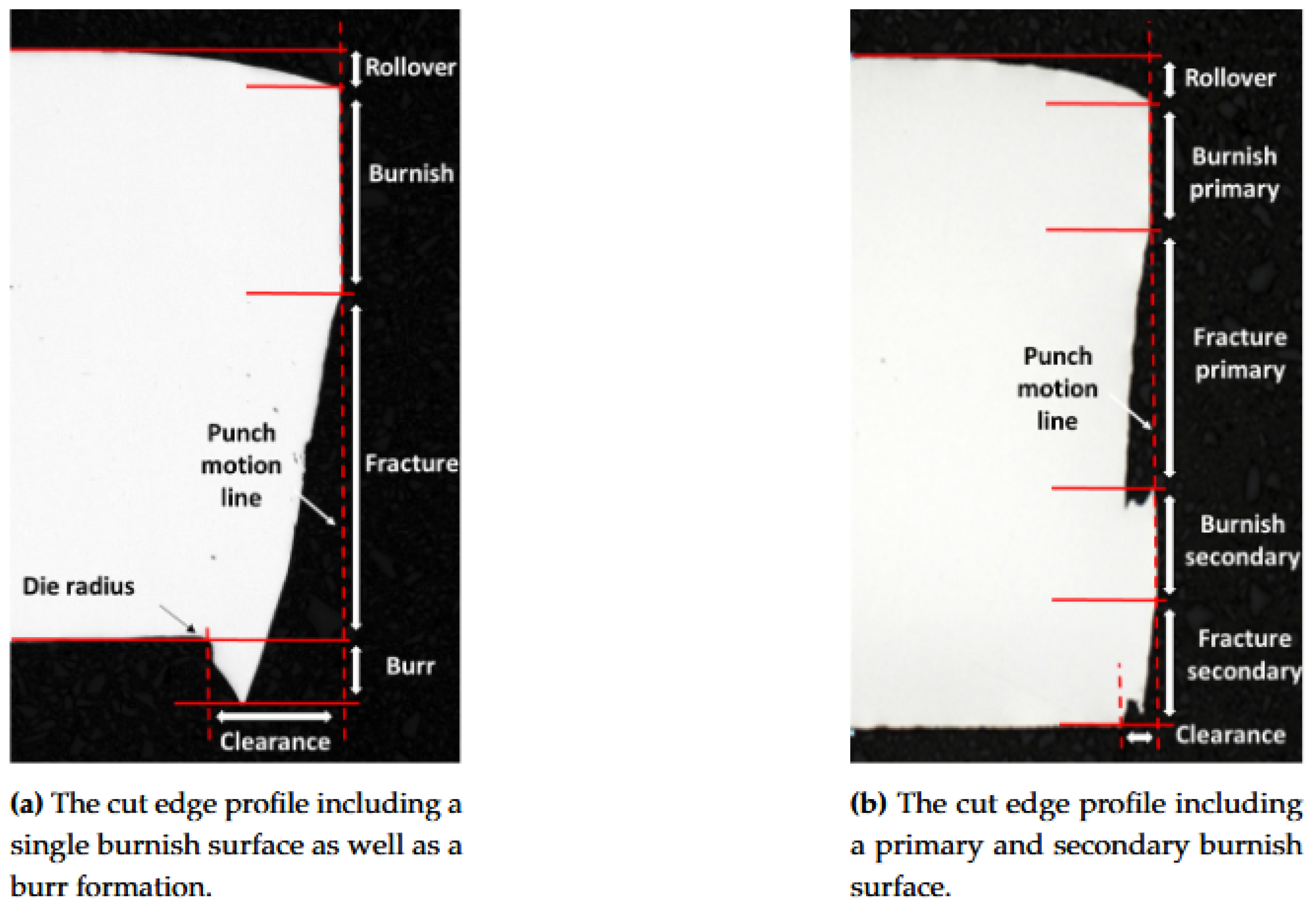
Figure 2.
Low/high magnification 2D/3D microscopy and metallographic cross sections of closed cut edges of AHSS sheets, showing formation of secondary burnish (left) and burr formation as well as rough fracture surface (right)
Figure 2.
Low/high magnification 2D/3D microscopy and metallographic cross sections of closed cut edges of AHSS sheets, showing formation of secondary burnish (left) and burr formation as well as rough fracture surface (right)
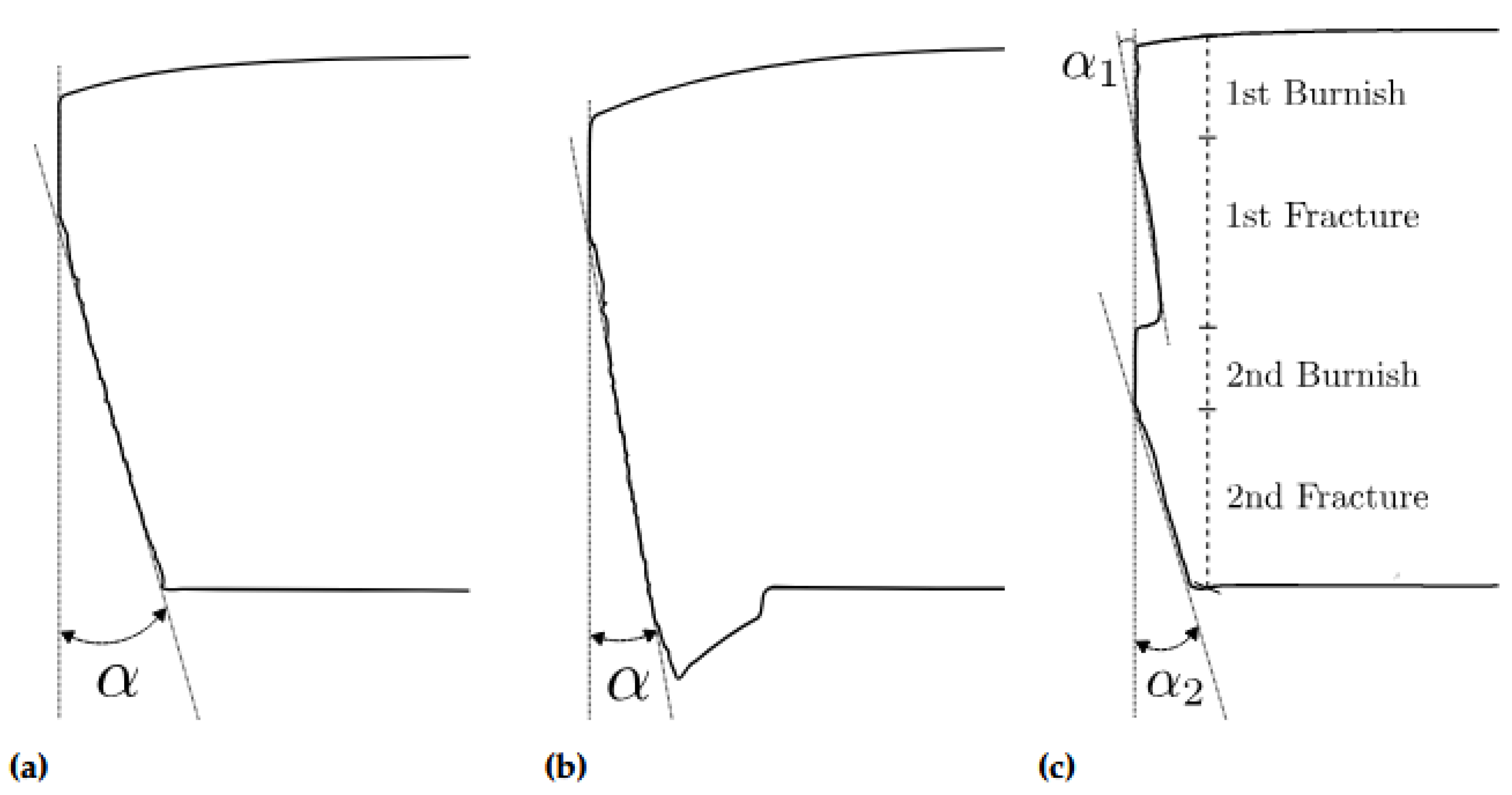
Figure 3.
Panoramic cut edges of open cut configurations using conventional cut edge investigation techniques, showing secondary burnish formation as well as full and partial burr formation of AHSS sheets.
Figure 3.
Panoramic cut edges of open cut configurations using conventional cut edge investigation techniques, showing secondary burnish formation as well as full and partial burr formation of AHSS sheets.
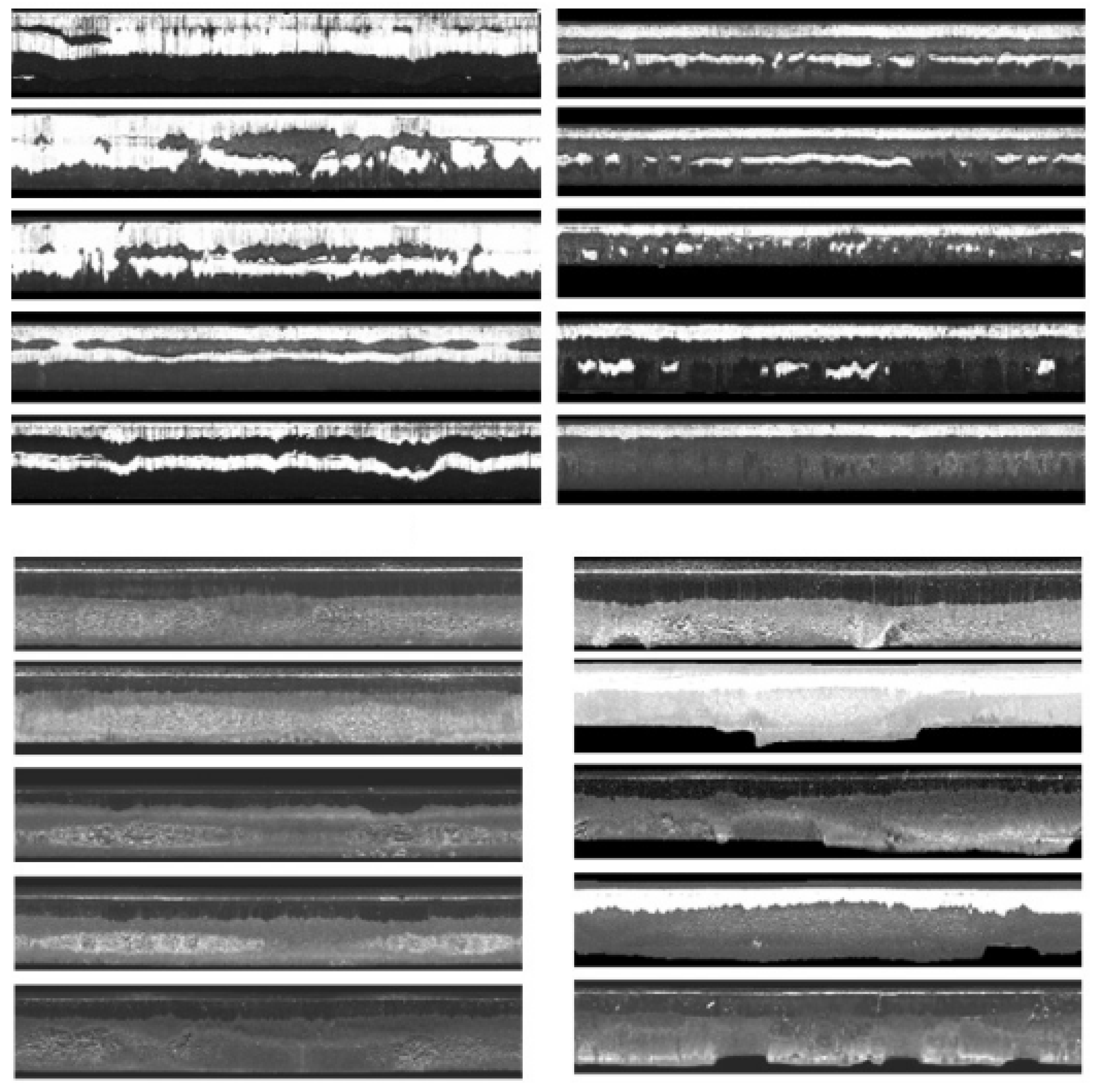
Figure 4.
In (a) the servo-hydraulic machine equipped with an ISO16630 dedicated hole punching tool. In (b) a schematic image of initial cutting configuration and in (c) a schematic image of finalized cutting.
Figure 4.
In (a) the servo-hydraulic machine equipped with an ISO16630 dedicated hole punching tool. In (b) a schematic image of initial cutting configuration and in (c) a schematic image of finalized cutting.
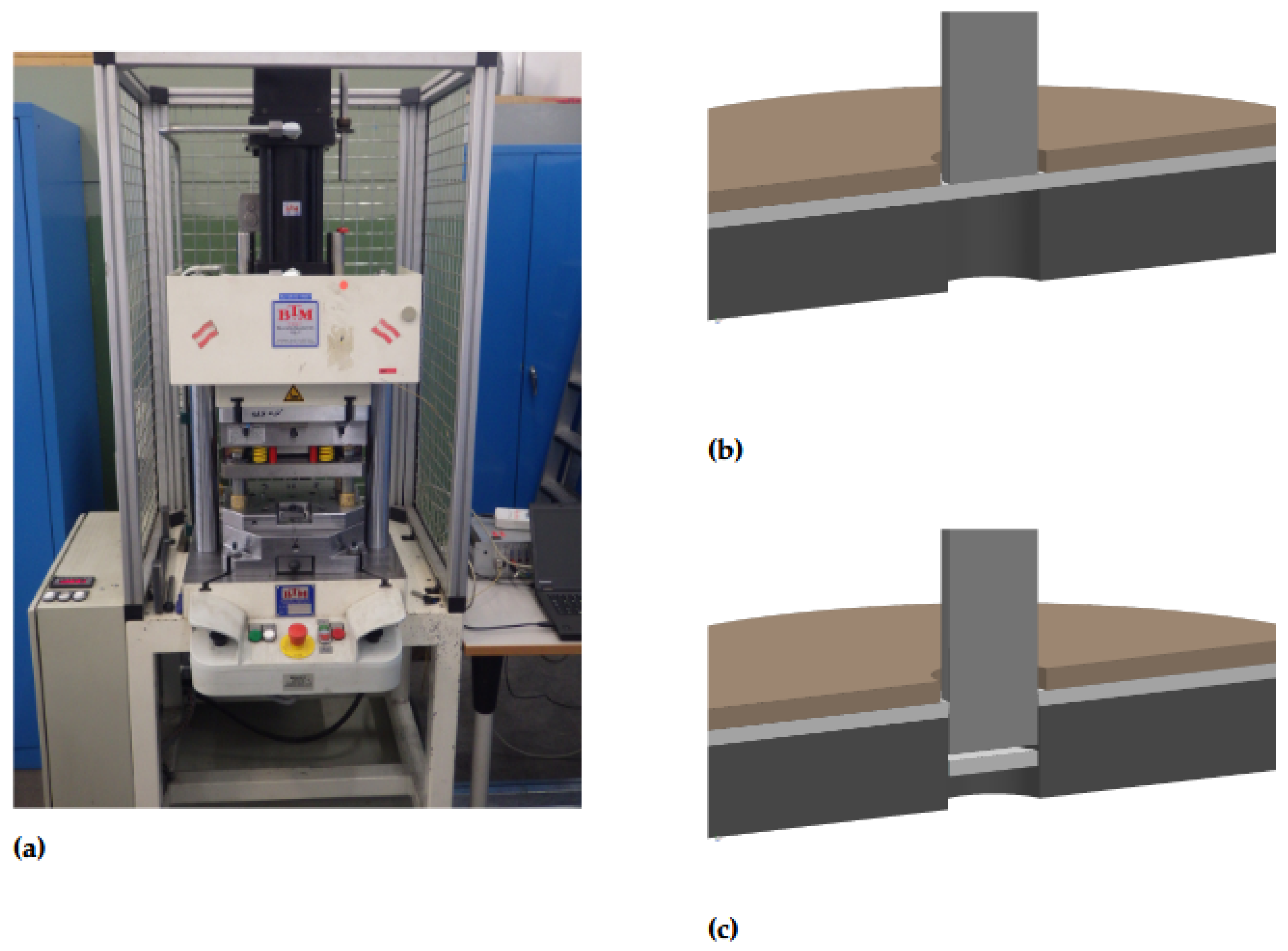
Figure 5.
Coaxiality test by paper punching, which shows the punch imprint at increasing punch displacement and a slight non-coaxiality through uneven cutting depth at 200 µm punch displacement.
Figure 5.
Coaxiality test by paper punching, which shows the punch imprint at increasing punch displacement and a slight non-coaxiality through uneven cutting depth at 200 µm punch displacement.
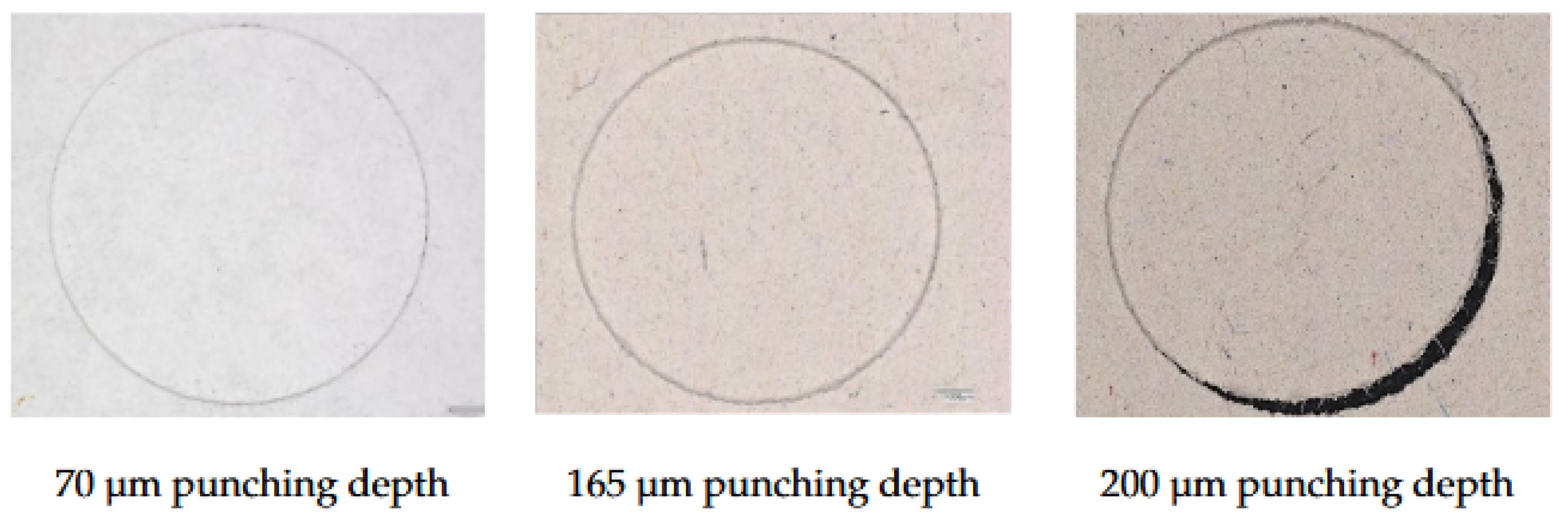
Figure 6.
Conventional cut edge investigation by (a) using x40-50 magnification USB digital microscope for qualitative cut edge and tools investigations and (b) metallographic cross section for cutting clearance determination.
Figure 6.
Conventional cut edge investigation by (a) using x40-50 magnification USB digital microscope for qualitative cut edge and tools investigations and (b) metallographic cross section for cutting clearance determination.
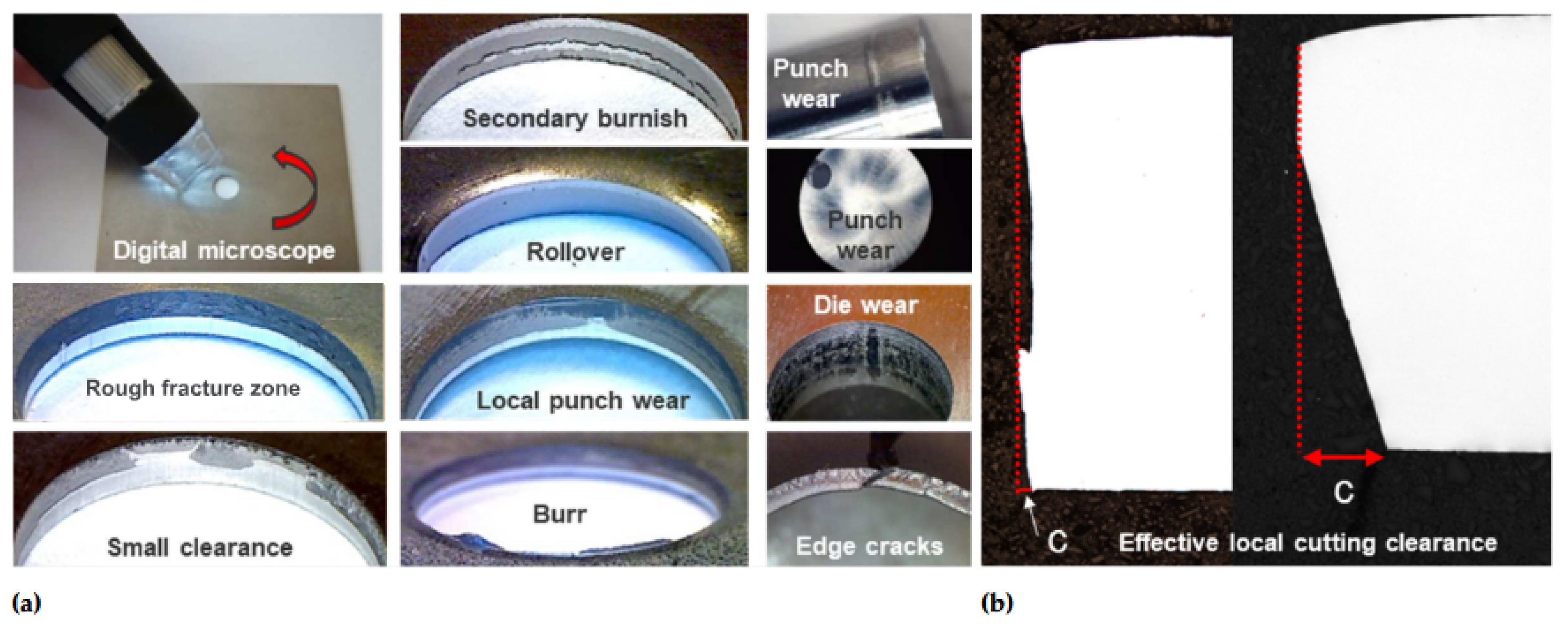
Figure 7.
The Edge Inspection System (EISYS) test set up, showing the pre-centring device in (a) and (b) used for positioning the punched sample. (c) shows the rotation table and (d) mirror at hole center.
Figure 7.
The Edge Inspection System (EISYS) test set up, showing the pre-centring device in (a) and (b) used for positioning the punched sample. (c) shows the rotation table and (d) mirror at hole center.
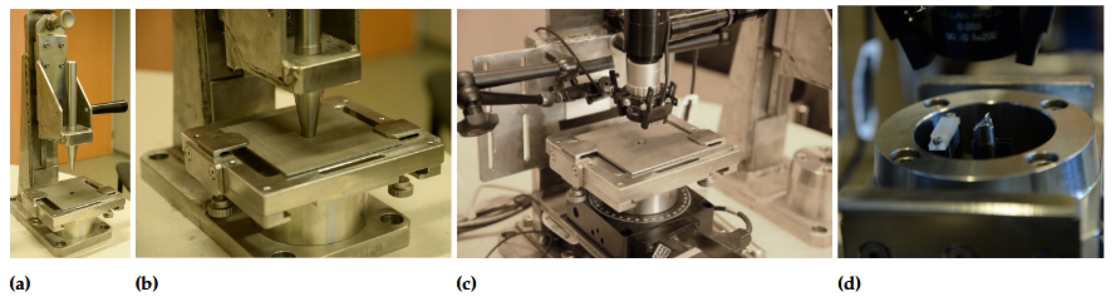
Figure 8.
The Edge Inspection System (EISYS) test set up in (a), showing the digitalization of the cut edge using the lightning concepts in (b)-(d).
Figure 8.
The Edge Inspection System (EISYS) test set up in (a), showing the digitalization of the cut edge using the lightning concepts in (b)-(d).
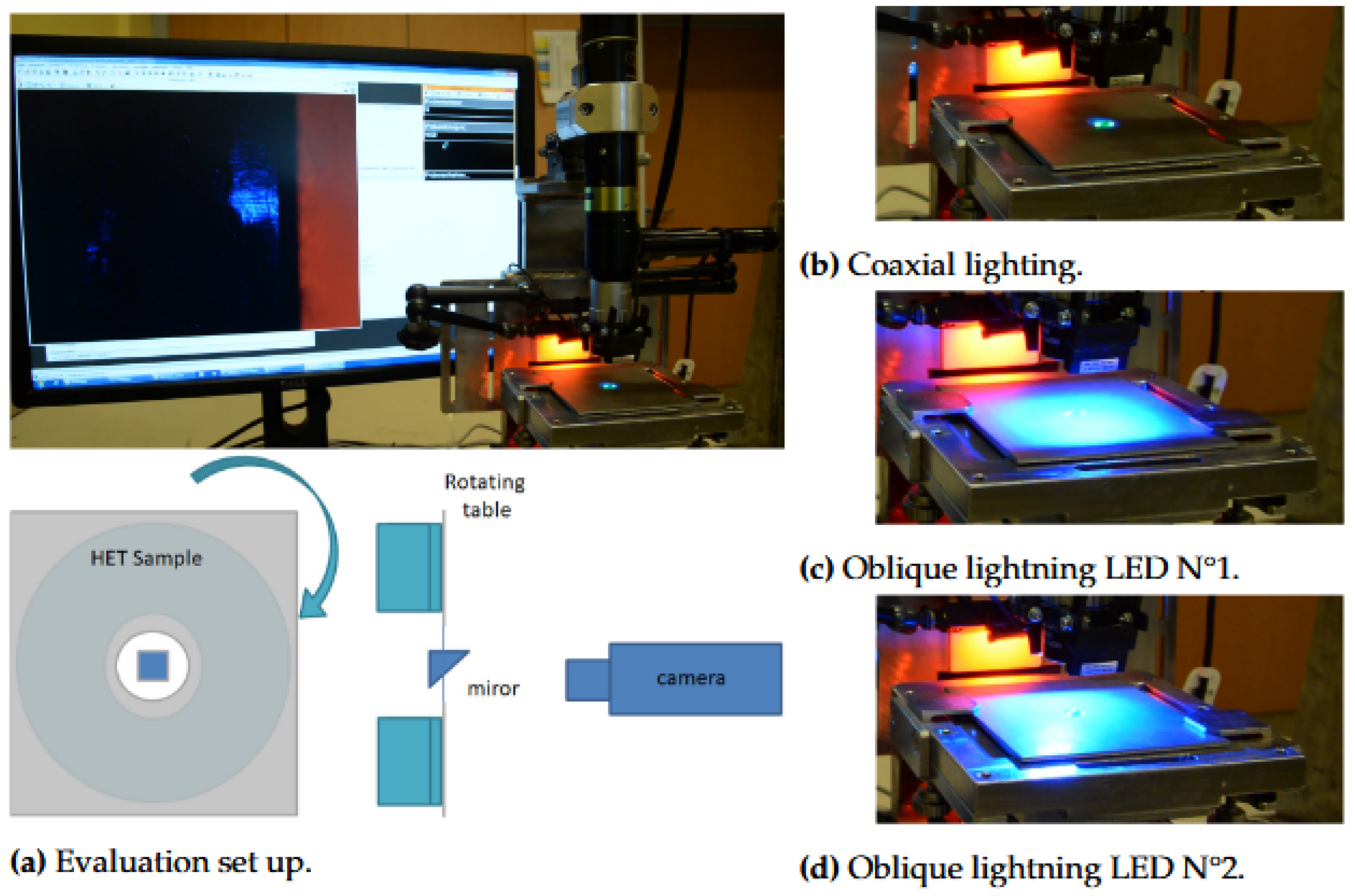
Figure 9.
panorama picture and cut edge parameter identification for 27% cutting clearance. After applying the EISYS approach, the panoramic images with varying lighting concepts in (a)-(c) were digitalized in (d). This enabled computation of the average distribution of the circumferential cut edge results in (e), along with the circumferential variation (standard deviation) as error bars.
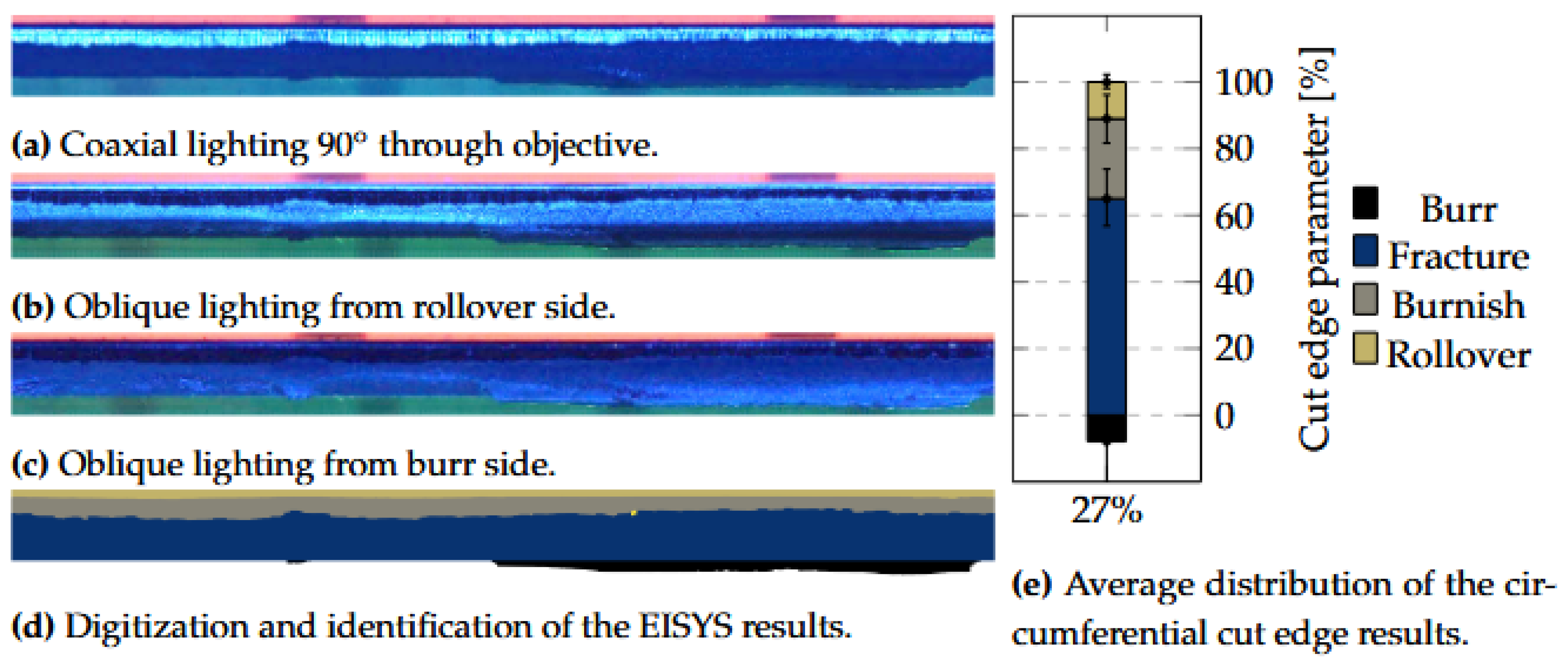
Figure 10.
The setup and and ingoing components used for the 45° mirror technique for stereo 3D microscopy. (a) shows the punched sample and the microscopy positioning, while (b) shows the 45° mirror and in (c) its placement in the punched sample. (d) shows the 45° view of the burnish- fracture edge profile during experimental investigation.
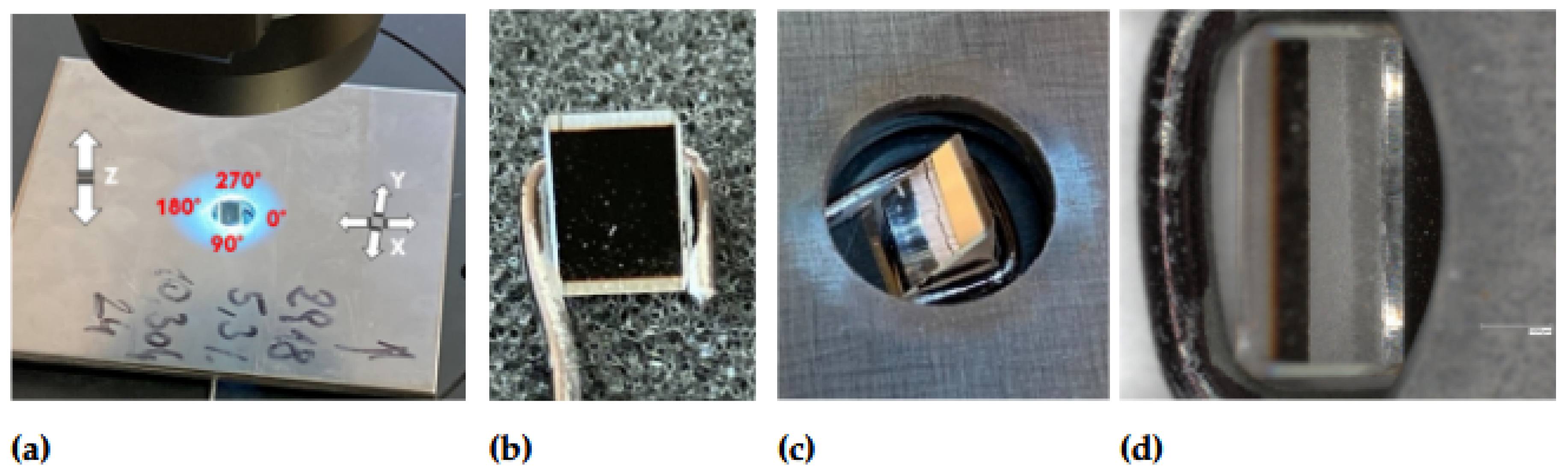
Figure 11.
In (a) the creation of rollover profile at the upper sample side. In (b) is the mirrored burnish-fracture profile of the cut edge front view and in (c) is the burr profile from the lower sample side. (d) shows the whole cut edge profile built by combining the individual top, down and front views.
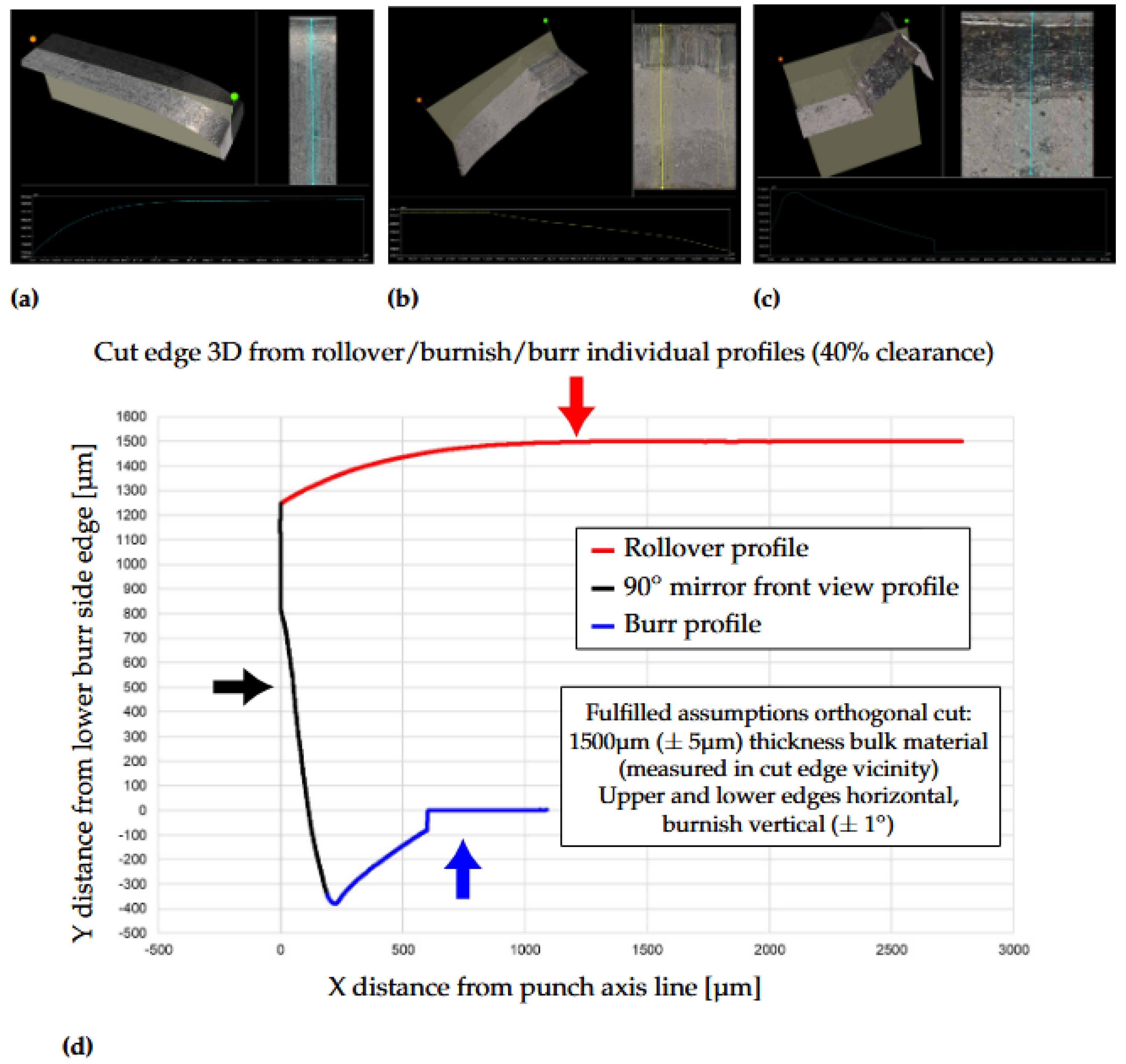
Figure 12.
The definitions of the fracture angles from (a) no burr condition, (b) with burr formation and in (c) with secondary burnish formation.
Figure 12.
The definitions of the fracture angles from (a) no burr condition, (b) with burr formation and in (c) with secondary burnish formation.
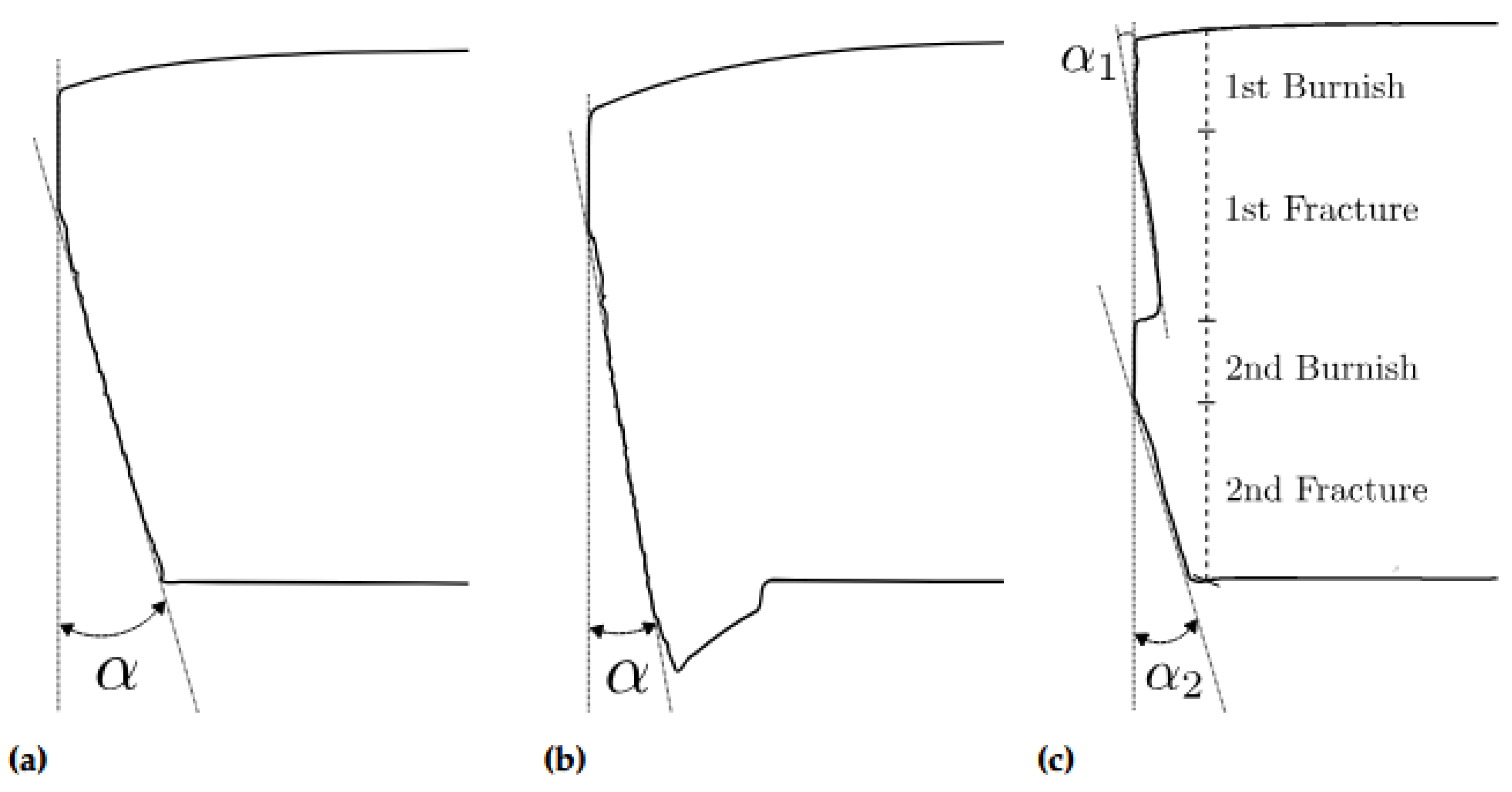
Figure 13.
The parallel indentation tracks used for Vickers hardness measurements of the 12% cutting clearance cut edge.
Figure 13.
The parallel indentation tracks used for Vickers hardness measurements of the 12% cutting clearance cut edge.

Figure 14.
The grain shear angle paths for the 12% cutting clearance cross section and the definition of the grain shear angle calculation along one of the defined paths. In (a) the etched cross section of a 12% cutting clearance cut edge, where six paths are highlighted with red lines along which the grain shear angles are determined. The red points show the measurement points where grain shear angle measurements were performed. In (b) a schematic image of the grain shear angle measurement following the burnish center path (red line) for the 12% cutting clearance cross section
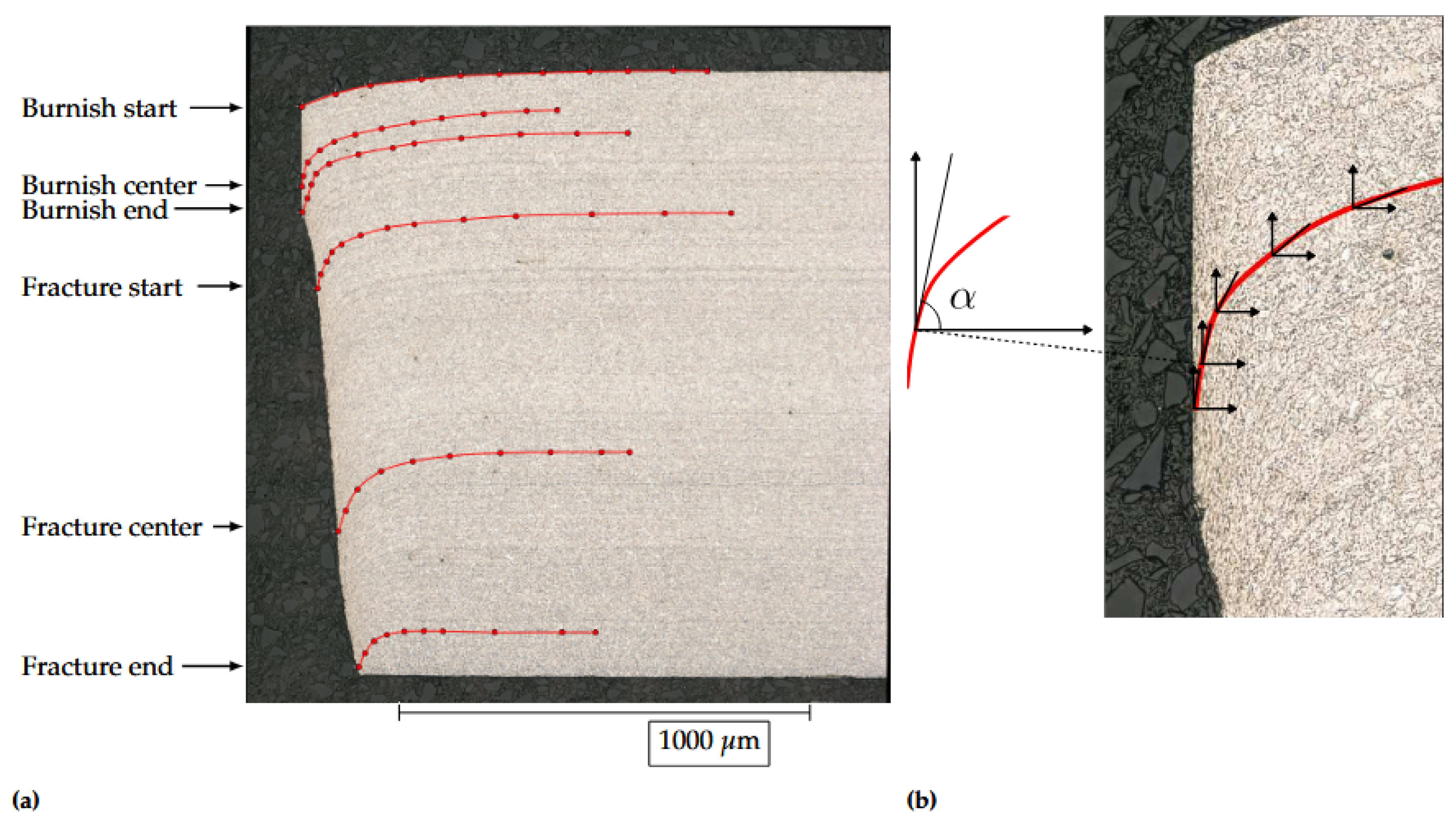
Figure 15.
A schematic image of grain shear angle results, where the scatter points represent the measured grain shear angles along an arbitrary path and the linear curves ( and ) show the linear fitting for distinguishing between localized shear deformation and global bending. The point shows the x-coordinate where the curves intersect, thus the width of the localized SAZ, the point of shows the critical angle at fracture and the point states the width of the total shear affected zone.
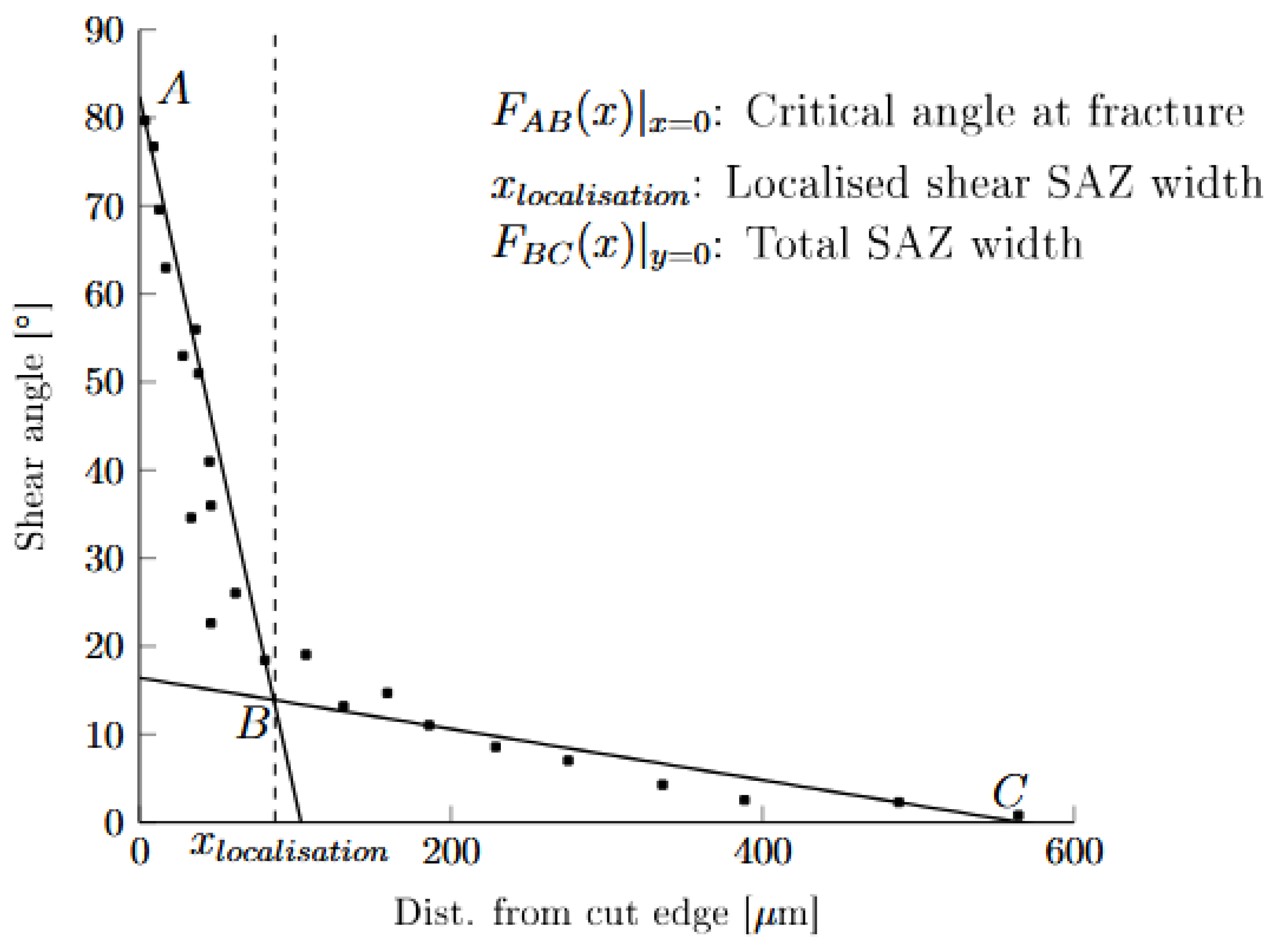
Figure 16.
Experimental cut edge profiles for different cutting clearances (Cl). The cut edge profiles were determined at , , and around the punched hole circumference. For 27%, additional cut edge profiles were extracted for providing information at no-burr and burr sections.
Figure 16.
Experimental cut edge profiles for different cutting clearances (Cl). The cut edge profiles were determined at , , and around the punched hole circumference. For 27%, additional cut edge profiles were extracted for providing information at no-burr and burr sections.
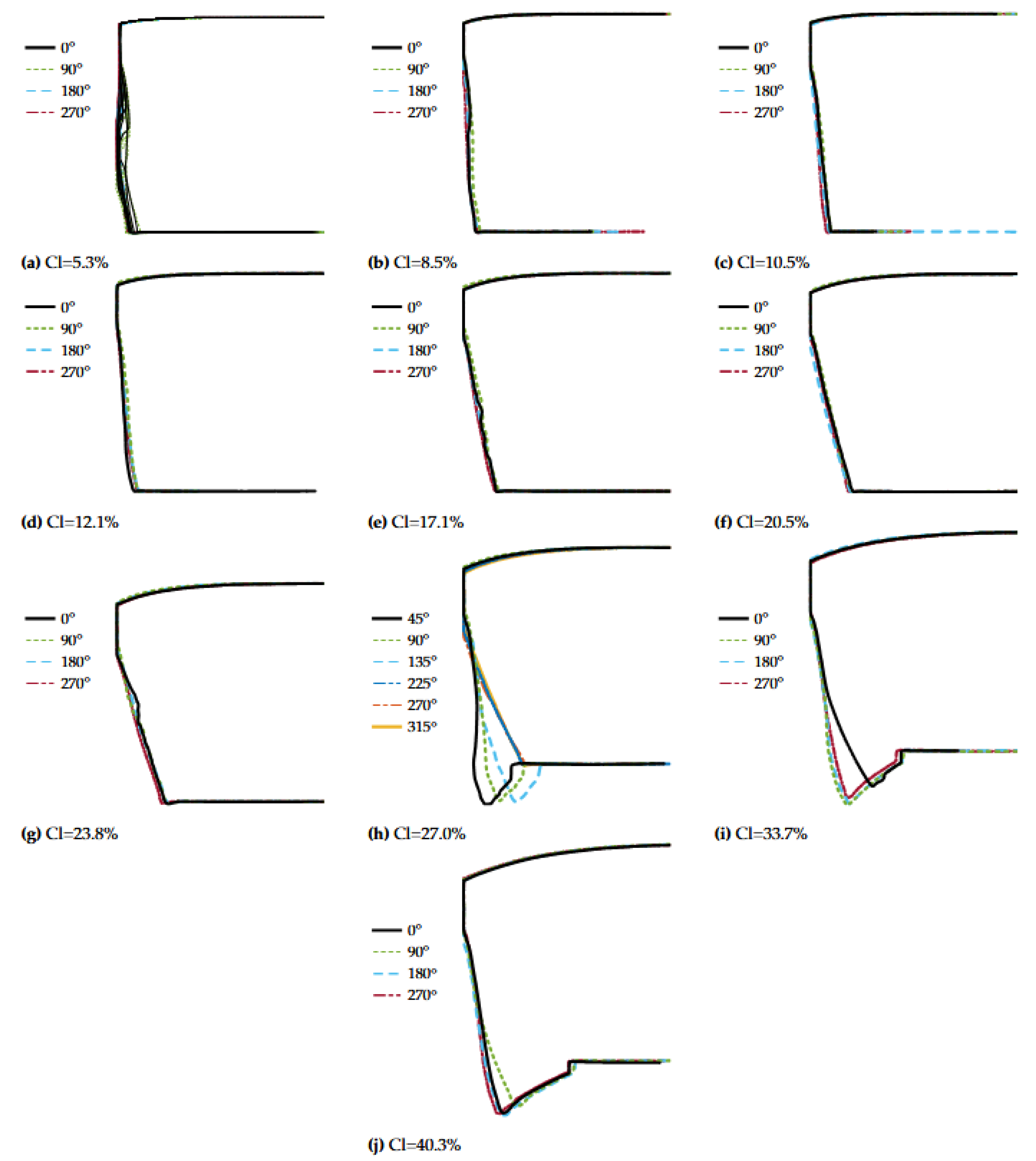
Figure 17.
Variation of cut edge profile at different positions along the hole perimeter produced by 5% cutting clearance. Each curve was extracted within degrees from the assigned position.
Figure 17.
Variation of cut edge profile at different positions along the hole perimeter produced by 5% cutting clearance. Each curve was extracted within degrees from the assigned position.
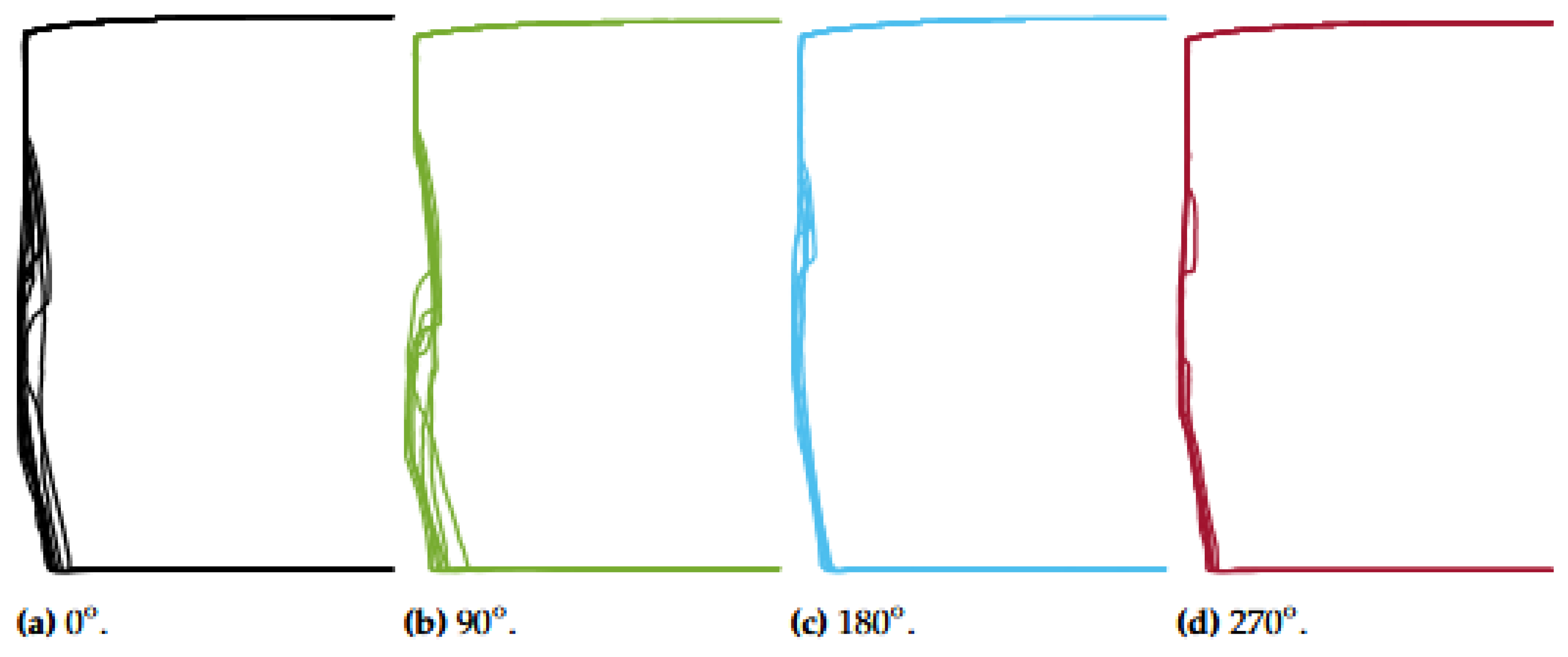
Figure 18.
Comparison of the cut edge profiles from the non-destructive 3D optical cut edge methodology (green lines) to destructive metallographic cut edge cross sections (images).
Figure 18.
Comparison of the cut edge profiles from the non-destructive 3D optical cut edge methodology (green lines) to destructive metallographic cut edge cross sections (images).
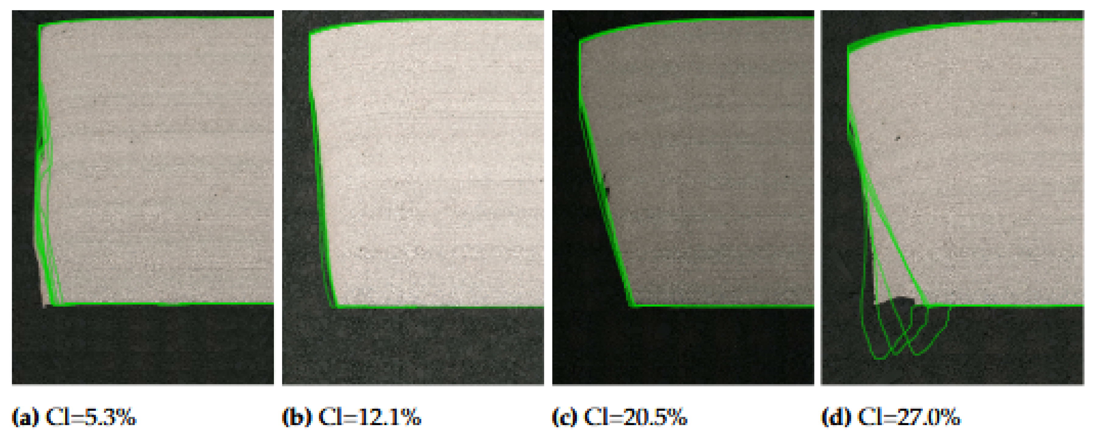
Figure 19.
Comparison between the 2D optical EISYS methodology and the metallographic cut edge cross sections, longitudinal to the rolling direction. The outer blank perimeters and the transition between the characteristic cut edge parameters are highlighted with red dashed lines.
Figure 19.
Comparison between the 2D optical EISYS methodology and the metallographic cut edge cross sections, longitudinal to the rolling direction. The outer blank perimeters and the transition between the characteristic cut edge parameters are highlighted with red dashed lines.
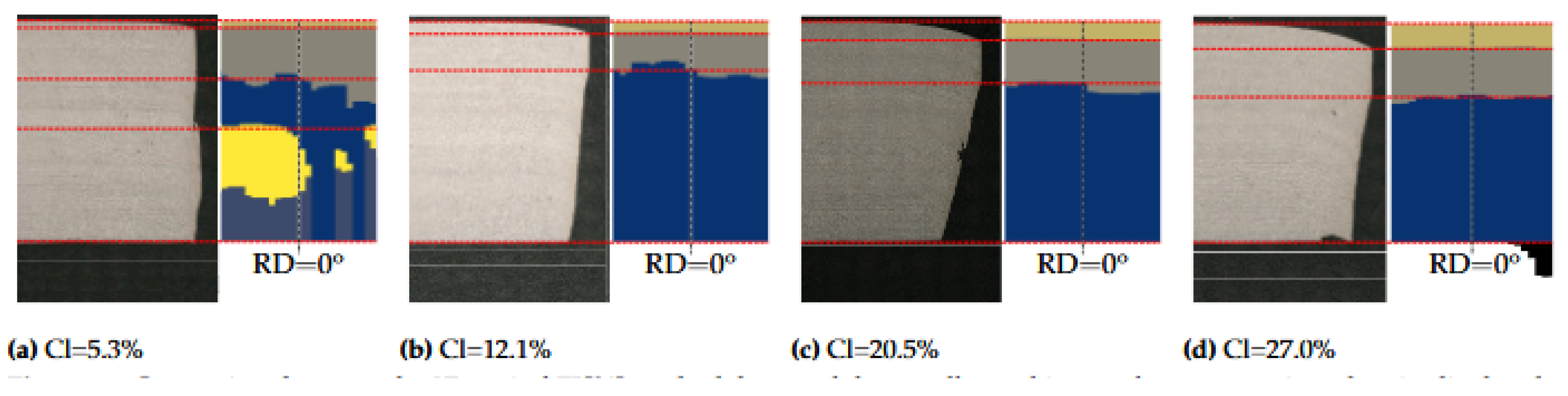
Figure 20.
Cut edge parameters versus cutting clearance, determined through the EISYS technique presented in Section 2.2.1.
Figure 20.
Cut edge parameters versus cutting clearance, determined through the EISYS technique presented in Section 2.2.1.
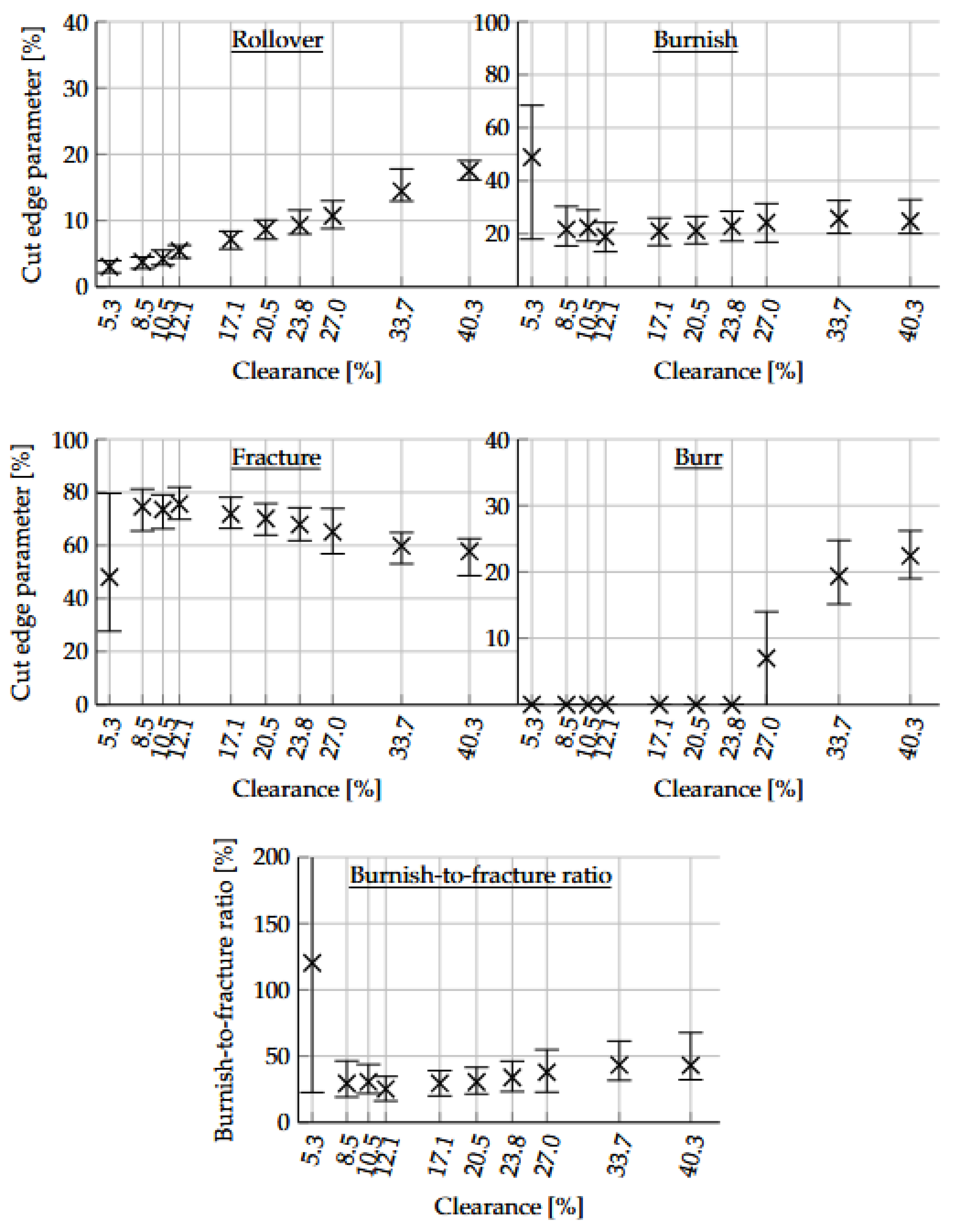
Figure 21.
Fracture angle measurements for varying cutting clearance at different positions around the hole perimeter.
Figure 21.
Fracture angle measurements for varying cutting clearance at different positions around the hole perimeter.
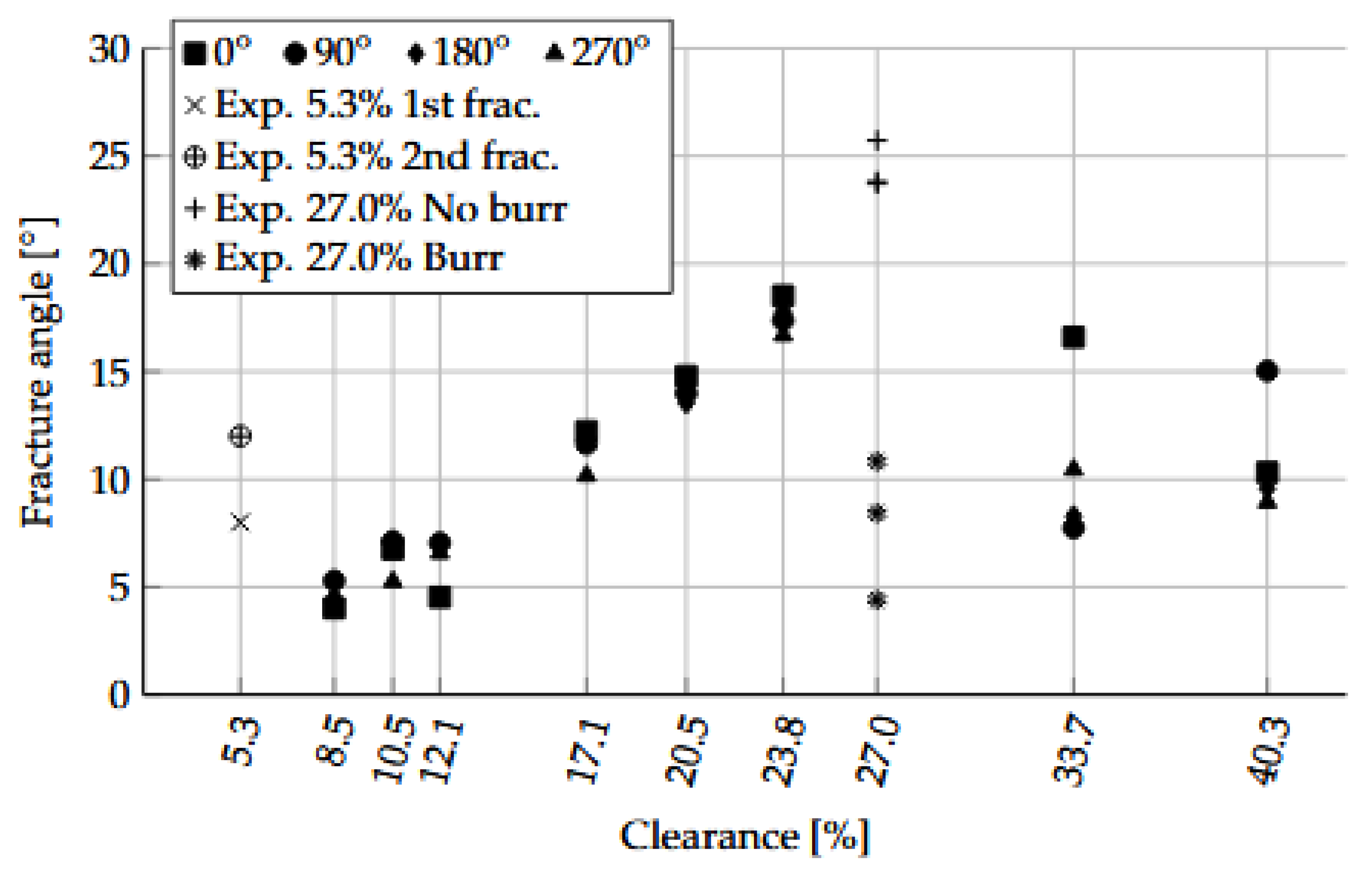
Figure 22.
Vickers hardness indentation results () plotted for each cutting clearance versus normalized distance from cut edge, combining three horizontal cut edge cross sections paths.
Figure 22.
Vickers hardness indentation results () plotted for each cutting clearance versus normalized distance from cut edge, combining three horizontal cut edge cross sections paths.
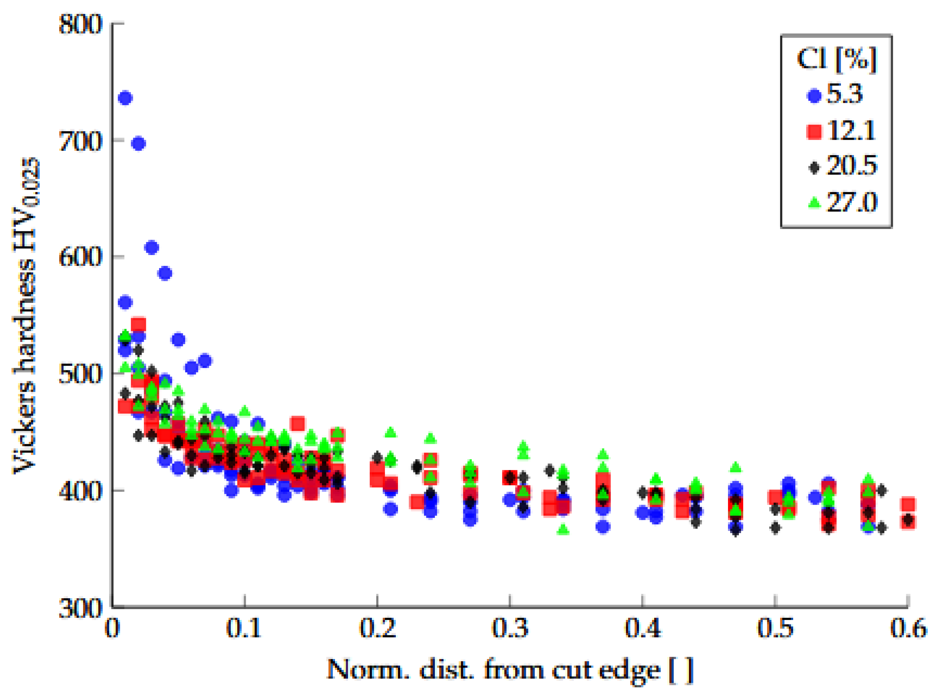
Figure 23.
Combined grain shear angle results from six extraction paths for 5%, 12%, 20% and 27% cutting clearances versus normalized cut edge distance.
Figure 23.
Combined grain shear angle results from six extraction paths for 5%, 12%, 20% and 27% cutting clearances versus normalized cut edge distance.
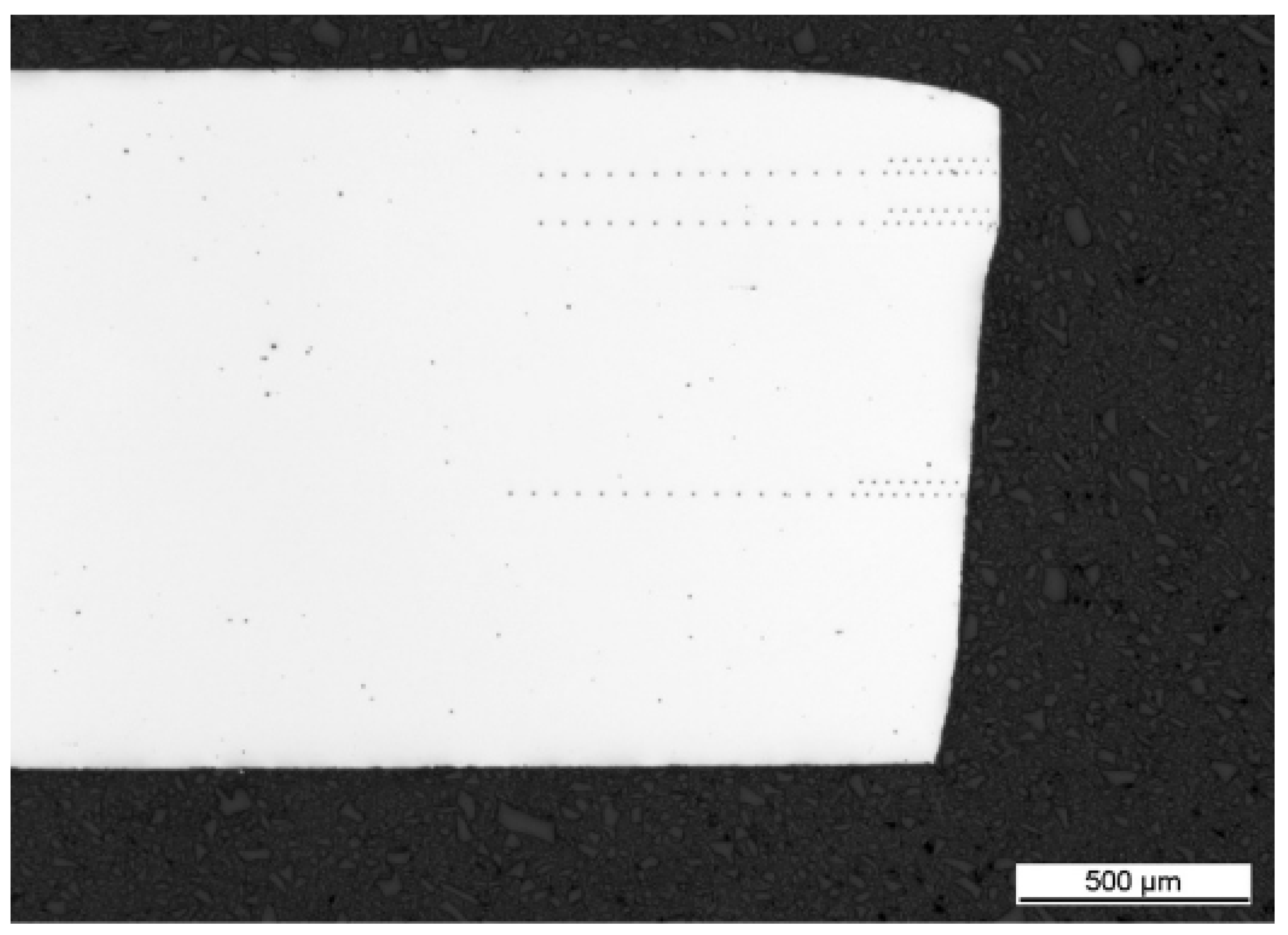
Figure 24.
Comparison between Vickers hardness (right vertical axis) and grain shear angle (left vertical axis) experimental results versus normalized cut edge distance for 12% cutting clearance.
Figure 24.
Comparison between Vickers hardness (right vertical axis) and grain shear angle (left vertical axis) experimental results versus normalized cut edge distance for 12% cutting clearance.
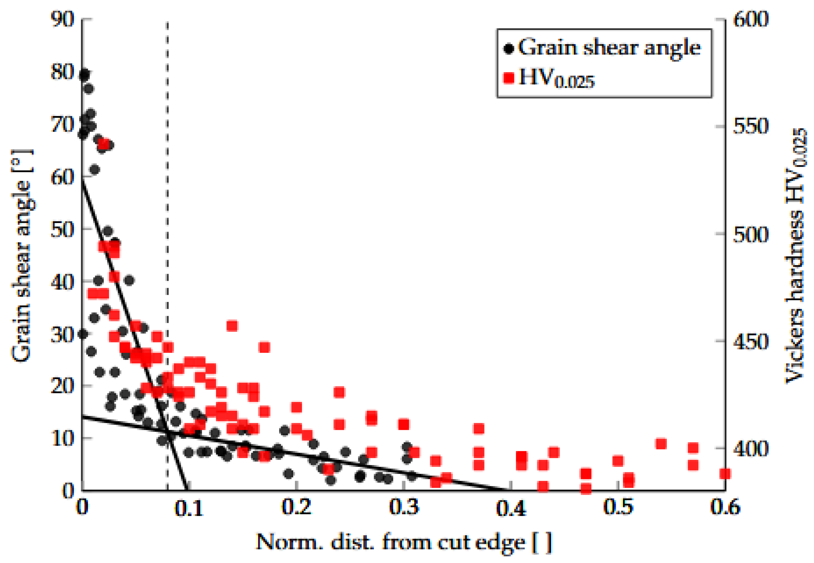
Figure 25.
Grain shear angle measurements for each individual path versus cut edge distance for 12% cutting clearance.
Figure 25.
Grain shear angle measurements for each individual path versus cut edge distance for 12% cutting clearance.
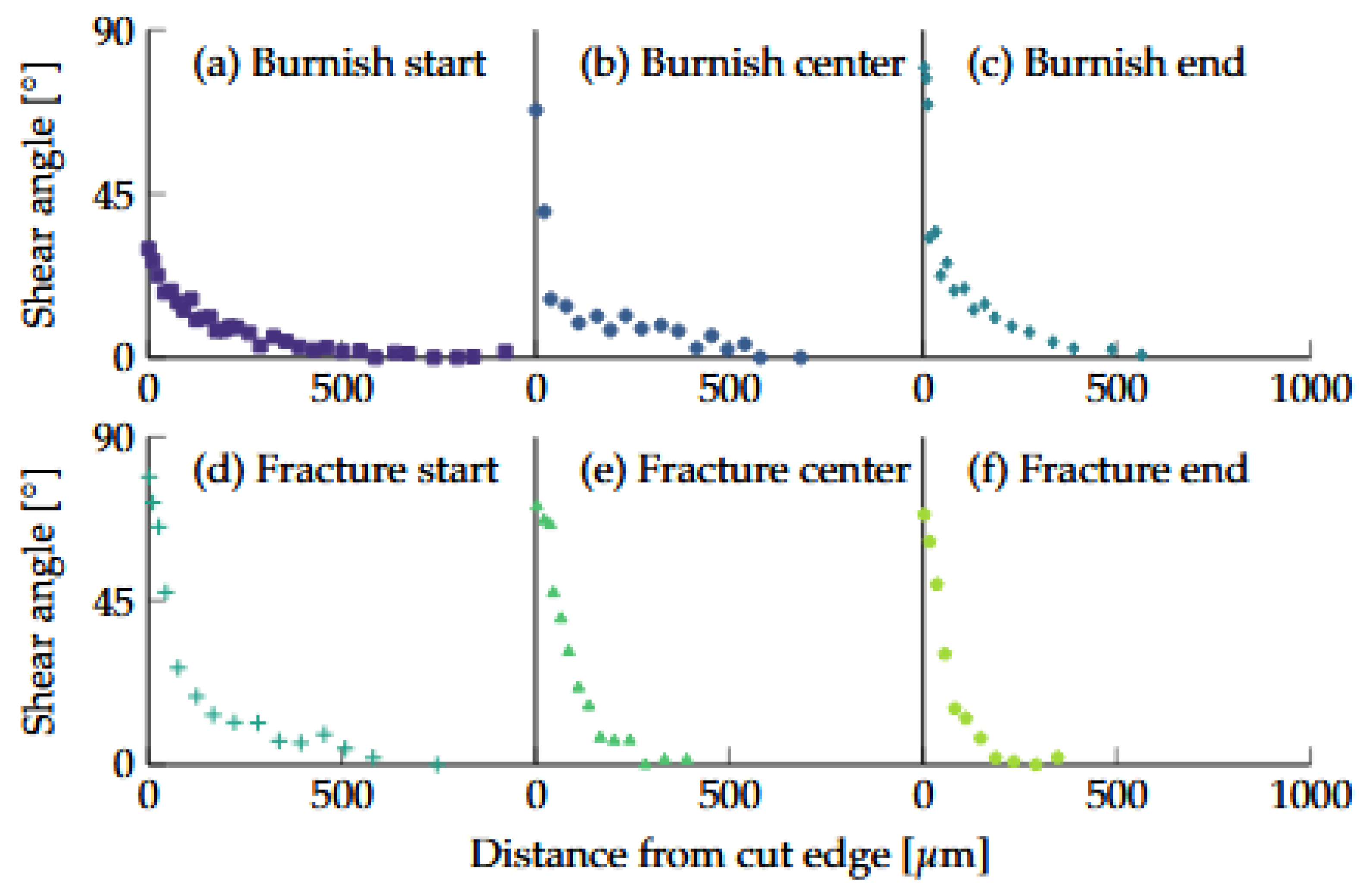

Table 1.
Mechanical tensile properties in different material directions relative to the rolling direction (RD) for CP1000HD with a thickness of mm, yield strength (), tensile strength (), uniform elongation (), total elongation () for 80 mm gauge length, n-value at uniform elongation () and r-value determined at 4% elongation ().
| RD | [MPa] | [MPa] | [%] | [%] | [-] | [-] |
| 893 | 1052 | 7.3 | 11.1 | 0.071 | 0.91 | |
| 905 | 1052 | 7.0 | 10.6 | 0.068 | 1.02 | |
| 909 | 1062 | 7.1 | 10.7 | 0.068 | 0.96 |
Table 2.
The geometric hole punching parameters used in experiments for clearances (Cl) 5-40%, where is the die diameter, is the punch diameter, is the die edge radius, is the punch edge radius and is the blank thickness.
Table 2.
The geometric hole punching parameters used in experiments for clearances (Cl) 5-40%, where is the die diameter, is the punch diameter, is the die edge radius, is the punch edge radius and is the blank thickness.
| Cl [%] | 5.3 | 8.5 | 10.5 | 12.1 | 17.1 | 20.5 | 23.8 | 27.0 | 33.7 | 40.3 |
| [mm] | 10.16 | 10.25 | 10.31 | 10.36 | 10.51 | 10.61 | 10.71 | 10.81 | 11.01 | 11.21 |
| [mm] | 9.998 | |||||||||
| [µm] | 30 | |||||||||
| [µm] | 30 | |||||||||
| [mm] | 1.5 | |||||||||
Disclaimer/Publisher’s Note: The statements, opinions and data contained in all publications are solely those of the individual author(s) and contributor(s) and not of MDPI and/or the editor(s). MDPI and/or the editor(s) disclaim responsibility for any injury to people or property resulting from any ideas, methods, instructions or products referred to in the content. |
© 2025 by the authors. Licensee MDPI, Basel, Switzerland. This article is an open access article distributed under the terms and conditions of the Creative Commons Attribution (CC BY) license (http://creativecommons.org/licenses/by/4.0/).
Copyright: This open access article is published under a Creative Commons CC BY 4.0 license, which permit the free download, distribution, and reuse, provided that the author and preprint are cited in any reuse.


