
Submitted:
26 May 2025
Posted:
26 May 2025
You are already at the latest version
Abstract
During reservoir development, asphaltene precipitation deposition triggers the blockage of seepage channels, significantly reducing the reservoir permeability and seriously affecting the effectiveness of water injection development and the operation efficiency of surface facilities. To alleviate this problem, this study proposes to use intermittent waterflooding (IWF) as an alternative strategy to improve reservoir dynamics by alternating periodic waterflooding and well shut-in operations. A synthetic reservoir model was developed based on the component simulator Eclipse 300, and the influence mechanisms of key parameters such as well shut-in time, injection rate, and injection start-up time were systematically investigated and compared and analyzed with the conventional water injection scheme. Numerical simulation results show that IWF can effectively suppress the amount of asphaltene deposition in the near-well zone. Early injection and higher injection rates can help maintain stable reservoir pressure and oil phase composition, thus limiting asphaltene precipitation. The study shows that optimizing the design of the intermittent water injection cycle helps improve the recovery rate and effectively reduces the risk of asphaltene formation damage, providing a practical water injection management strategy for high-risk reservoirs.
Keywords:
Intermittent waterflooding
; Asphaltene deposition
; Reservoir simulation
; Enhanced oil recovery
; Sensitivity analysis
; Floculation
1. Introduction
As the oil industry increasingly relies on enhanced oil recovery (EOR) techniques to maximize production from mature reservoirs, flow assurance problems associated with crude oil components have become a major concern [22]. Water injection is a widely used and cost-effective secondary oil recovery method used to maintain reservoir pressure effectively [18]. However, conventional continuous water injection tends to reduce the solubility of heavy components due to pressure and component variations, which induces asphaltene precipitation (Carrera et al. [2]). Precipitated asphaltenes can clog pores, reduce permeability, damage reservoir rock structure, and even damage surface equipment. Fahes et al. [3] showed that even the presence of only trace asphaltene deposits can significantly reduce the flow capacity of sandstone cores, and Khurshid et al.6 further found that continuous water injection may lead to dissolution and redeposition of rock minerals, formation of cement, and exacerbation of reservoir plugging. While factors such as mineralization, pressure fluctuation and water injection period also have significant effects on the location and scale of asphaltene deposition [13]. Several recent works have utilized similar simulation tools to study asphaltene effects: for example, Milad et al. (2022) [8] conducted core-scale experiments and history-matched simulations to examine how flow rate and pressure influence asphaltene deposition in porous media.
In order to mitigate asphaltene-related problems, researchers have proposed a variety of preventive and management tools, including controlling the magnitude of pressure drop, injecting aromatic solvents (e.g., toluene), using surfactants, nanofluids, and chemical inhibitors [10]. However, Shekarifard et al [11]. pointed out that solvent flushing, mechanical removal and ultrasonic treatment are difficult to apply on a large scale due to high cost and environmental impact factors. In recent years, intermittent waterflooding (IWF) has gained attention as an active modulation strategy, which helps to stabilize reservoir conditions and retard asphaltene generation and deposition by alternating injection and shut-in phases [18]. In particular, Khurshid et al. [6] emphasized that the injection rate and the injection period have a significant effect on the depositional behavior, and their “huff-and-puff” model shows that frequent fluctuations may exacerbate the deposition, which demonstrates the importance of optimizing the parameters of the injection operation.
Asphaltenes are polymeric organic compounds insoluble in light alkanes but soluble in aromatics and are usually thermodynamically stable in crude oil in the form of micelles [1]. When temperature, pressure, or oil phase components change, the stability is destroyed, leading to precipitation and deposition [9]. In water-injected reservoirs, deposition triggers include 1. pressure drop near injection wells directly triggers precipitation [6]; 2. component differentiation increases local asphaltene concentration [1]; 3. salinity, pH, and divalent cations (e.g., Ca²⁺, Mg²⁺) in the injected water interact chemically with asphaltene and accelerate precipitation (Khurshid et al. 20186). Deposition mostly occurs near water injection wells and oil sweep zones, resulting in increased injection pressure, reduced permeability, earlier water breakthrough, and decreased replacement efficiency. In addition, asphaltene deposition can change rock wettability from water to oil wetting and increase crude oil retention [16].
To address these issues, mainstream simulators such as Eclipse and CMG GEM integrate models of particle surface deposition, entrainment transport, and plugging mechanisms, combining equation of state (EOS)-based thermodynamic deposition with the dynamic evolution of porosity and permeability [9]. Khurshid et al. (2018) [6] further extended the model to include dissolution and redeposition of rock minerals, successfully simulating water injection-induced permeability impairment. Although asphaltene behavior is highly sensitive to system conditions, compositional simulation tools provide engineers with an effective “hypothesis-testing” platform to evaluate the effects of operational parameters such as injection rate, start-up time, and cycling mode on asphaltene deposition [8].
The purpose of this paper is to investigate an operationally flexible asphaltene control strategy, the intermittent waterflood (IWF) method. This method regulates reservoir pressure and oil-phase composition prior to asphaltene deposition by cyclically alternating water injection and well shut-in, thereby delaying particle aggregation and deposition [18]. Although IWF has been successfully applied in souring and thermal oil recovery, there is a lack of systematic research on asphaltene control [20]. Therefore, in this paper, based on the Schlumberger Eclipse 300 compositional simulator, we designed and compared continuous water injection and IWF scenarios, and evaluated the effects of key parameters, such as well shut-in time, injection rate and cycle duration, on depositional evolution and recovery efficiency. This paper also explores the sensitivity and optimal operation window of IWF, which provides a practical reference for oilfield practice8.
2. Mitigation Strategies and Modeling Framework
The Asphaltene option in Eclipse 300, the reservoir simulator created by Schlumberger that was used for this research, models asphaltene behavior in a reservoir. There are more sophisticated thermodynamic models, such as the Flory-Huggins regular solution theory (modeling asphaltenes from a polymer perspective), Peng-Robinson or SRK-based extensions of the equation of state (considering the solid-phase stability envelope), and the PC-SAFT (Perturbed Chain Statistics). theory), which models intermolecular interactions and polydispersity effects. Mohebbinia et al. (2017) [9] successfully reproduced the nonlinear precipitation-redissolution behavior during gas injection via PC-SAFT for a one-time depletion scenario where asphaltene precipitation is not observed. Engineering, the colloidal instability index (CII) was used for the initial assessment of asphaltene stability, defined as:
The system tends to be unstable when CII > 0.9 and more stable when CII < 0.7, but this metric is not applicable to the prediction of precipitation under dynamic conditions such as water injection.
Asphaltenes precipitate and first form fine particles suspended in the oil, which may subsequently aggregate to form flocs. denotes the concentration of precipitated fines coming from component i. denotes the concentration of the flocculated components. Eclipse uses a kinetic model to simulate this flocculation process in the form of:
where is the aggregation rate of the fines i into flocs and is the flocculation rate coefficient, and is the dissociation rate coefficient.
The flocculated particles can migrate, adsorb or deposit in the core. The modeling equations for depositional behavior are as follows:
The variable d denotes the dimensionality of the problem, while εᵢ represents the volume fraction of deposited solids along the flow direction i. The parameter α serves as the adsorption or static deposition coefficient, describing how readily flocs adhere to the pore walls. Φ indicates the current porosity of the medium at time t, which evolves as deposition progresses. Cₐ is the volumetric concentration of asphaltene flocs suspended in the oil phase, and Fₒᵢ is the Darcy flux of the oil in direction i. The γ parameter quantifies the plugging coefficient, reflecting the extent to which deposited flocs reduce permeability, while β is the entrainment coefficient governing the remobilization of previously deposited material. Uₒᵢ denotes the local oil-phase velocity, and U_cr is a user-defined critical velocity threshold. Importantly, the presence of a “+” symbol outside the velocity-related term implies that entrainment will only occur when the absolute oil velocity exceeds this critical value; otherwise, the entrainment contribution is set to zero. The overall volume fraction of deposit in i directions is formulated as:
The mole fraction of the flocs that deposit is:
And the mole fraction of the flocs that remain suspended in the oil is:
The concentration of the flocs which are flowing with the oil phase are taken as:
Where bₒ represents the oil molar density, Sₒ is the oil saturation, and xₐ denotes the molar fraction of flocs in the liquid phase. The ASPDEPO keyword is used in the data file under the PROPS section to specify the values of α, γ, β, and U_{cr}. These parameter values are typically obtained from laboratory core flood experiments using fluid samples extracted directly from the reservoir.
When the ASPLCRT keyword is not initiated in the data file, these critical values are both set to zero. The deposition model can be altered to include plugging as follows:
Where:
γ = γ if ε>εcr and/or Ca>Cacr
γ = 0 if ε<εcr and/or Ca<Cacr
The average pore radius will decrease as the critical volume fraction of asphaltene deposition is reached. A critical radius than then be defined as:
Where δ is a user input. The remaining flow radius then becomes:
The critical floc concentration can be thought of as the point above which the size of individual flocs is large enough to plug pore throats during flow. The critical volume fraction of deposition can be interpreted as the value above which deposition is likely to cause plugging of pore throats.
Decrease in porosity is one of the many types of damages that can occur due to asphaltene deposition. This reduction in porosity can be determined as:
Where Φo is initial porosity and ε is volume fraction of asphaltene deposition.
Experiments have shown that sedimentation has a relatively small effect on porosity but a significant effect on permeability. The permeability damage is then taken as a parametrized power law quantified by:
Where is a user input, k is permeability at time t, ko is initial permeability.
Oil viscosity will change as asphaltenes precipitate and deposit. The change in viscosity is caused by the introduction of colloidal fines during precipitation and loss of oil phase components during deposition. The third argument of the ASPHALTE keyword will determine which of three models will be used to quantify viscosity changes. The ASPVISO keyword is used in conjunction with these arguments to specify parameter values of the three models. The following three models may be used to quantify changes in viscosity:
- 1)
- Einstein Model (one parameter)
This model is applicable to low concentrations of asphaltene, and a is slope of relative viscosity with respect to volume concentration of precipitate, and Cp is the volume concentration of precipitate, and μo is the oil viscosity at Cp=0, and μ is the current oil viscosity.
- 2)
- Krieger–Dougherty Model
Where is the intrinsic viscosity, and Cpo is the volumetric concentration for maximum packing.
- 3)
- Tabulated Data
A look-up table may be utilized rather than a formulated model to determine oil viscosity changes. The third argument under the ASPHALTE keyword is TAB for this model. The ASPVISO keyword is used to input the look-up table. This table lists oil viscosity multipliers as a function of the mass fraction of precipitate. The table values can be determined from laboratory experiments on an oil sample. Extrapolation is used to determine values between sets of table data. However, if a mass fraction value is outside of the bounds identified in the table, no extrapolation is made and the nearest viscosity multiplier is applied.
All three models are configured by ASPVISO to dynamically update the oil phase viscosity for each grid. the IWF strategy allows for re-dissolution of asphaltenes, reduction of and viscosity, and restoration of mobility during periods of water shutdown. Continuous water injection often leads to accumulation, reduced mobility, and increased plugging. Therefore, the viscosity model plays a bridge role in the integrated modeling of asphaltene, effectively coupling the fluid state with the physical changes of rocks.
3. Results Analysis
Eclipse 300 is used to study the effects of asphaltene in a 3D reservoir during production and intermittent waterflooding for this study. The “Asphaltene Option” is enabled in the data file in order to activate the asphaltene model. The “Asphaltene Option” in Eclipse 300 has the capability of combining a theoretical model with experimental data.
The reservoir is constructed as a 40 X 3 X 6 grid. Each block in this grid has a length (dx) of 250 feet, width (dy) of 1000 feet, and a thickness (dz) of 15 feet. The porosity is taken to be homogenous at 15% across the entire reservoir. The permeability is also homogenous in the x and y direction at 500mD. However, the permeability in the z direction is taken to be a lesser value of 300mD. For more details on the properties of the reservoir model or oil composition, the data file in the Appendix can be referenced.
Figure 1.
Initial Oil Saturation. This figure shows the oil saturation in the reservoir before production and injection.
Figure 1.
Initial Oil Saturation. This figure shows the oil saturation in the reservoir before production and injection.
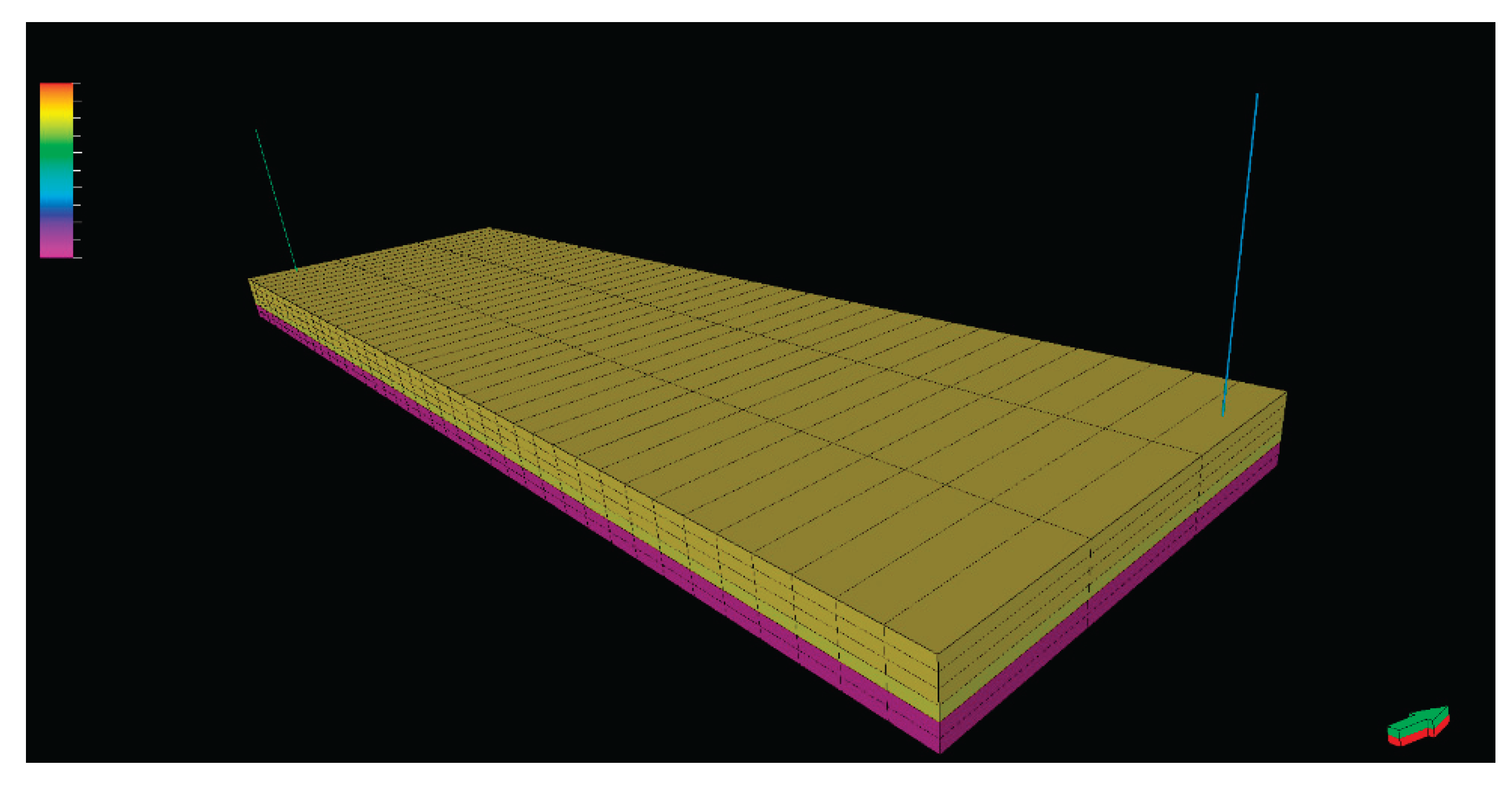
Figure 2 illustrates reservoir interaction over time, using data from the reservoir midpoint to show median conditions. Initially, oil pressure drops steadily until around 2300 psi, corresponding to the bubble point, where the rate of pressure decline changes. Gas saturation is shown for layers 1 and 2: layer 1 shows variation, while layer 2 remains at zero throughout. Asphaltene deposition increases sharply near the bubble point. The rise in oil pressure marks the start of the intermittent waterflood. Its effects align with periods of injection, as reservoir pressure rises near the new bubble point, reducing free gas saturation. Asphaltene deposition initially increases, likely due to temperature changes, but later decreases as thermal equilibrium is approached. The final depletion phase begins when pressure drops after the waterflood. Free gas saturation quickly rises, indicating an increased bubble point from compositional changes. Asphaltene deposition is mitigated, breaking the earlier trend of increasing deposition rate.
3.1. Reservoir Shut-In Time Sensitivity
Figure 3 illustrates the sensitivity analysis conducted for this experiment. The time period for which the reservoir was completely shut in is varied. This shut-in time is the period between the end of the intermittent waterflood and the second production period, where the reservoir is completely closed off from flow. This time period was set to 800 days and the asphaltene deposition was monitored in certain cells. It was shown that the net deposition should remain constant over the full period of 800 days. This sensitivity analysis was conducted to draw a conclusion based on this observation, and assert that the producer should be open much earlier than 800 days following the intermittent waterflood.
3.1.1. Asphaltene Deposition
Deposition occurring during depletion can be attributed to pressure changes. Reservoir depletion causes reduction in pressure and therefore changes kinetic energy. This destabilizes the colloidal particles causing precipitation which leads to deposition. The precipitated particles will aggregate and form flocs. Some of these flocs will be held in suspension while others will deposit due to further destabilization.
It is also observed that deposition is increasing during injection. This can be attributed to temperature changes in the reservoir. The reservoir temperature is 160°F, while the temperature of the water being injected is taken as surface conditions (60°F). This causes a temperature change in the reservoir during the waterflood process. The temperature change is another kinetic energy change which results in deposition.
Figure 4, Figure 5 and Figure 6 show that final net asphaltene deposition remains relatively constant at the end of each simulation of varied shut in time. However, there are very small changes observed as the shut-in time is varied. These small changes stem back to effects of pressure change that can be observed in Figure 3. The pressure is shown to continually drop be a few psi over the extent of the entire year of varied shut-in time in Figure 3, even though the system is completely shut off from flow in or out. This is likely due to some type of simulator error where the simulation is trying to bring the system into equilibrium but failing to do so. These small changes should occur over the first hours, or days, which is the amount of time it takes for such a system to reach equilibrium. These small changes should not occur over the time period of a year and there is no physical explanation for this occurrence. However, the changes in deposition are still so small that they can be considered negligible. Therefore, it is logical to conclude that the reservoir should be open for production within the first week following the intermittent waterflood to benefit economic feasibility.
3.1.2. Permeability Damage
Figure 7, Figure 8 and Figure 9 illustrate how permeability is affected for each shut-in time at different locations. Permeability damage is shown as a multiplier, where the actual value of permeability is just the multiplier into the initial permeability. Lower values of the multiplier therefore indicate higher permeability damage. Permeability is based on a function of deposition, and as such it is expected to decrease as deposition increases. The results are consistent with this theory. The results also show that very insignificant changes to permeability occur between each shut-in time due to the issues preventing the simulation from reaching equilibrium.
3.1.3. Plugging
Asphaltene deposition is related to plugging by flocculation. Deposition occurs as flocs are aggregated and transferred to the rock surface. Plugging is considered part of the deposition that occurs as flocs clog pore throats during fluid flow. Therefore, both plugging and deposition are expected to follow similar trends since they are governed by flocculation. The results of this simulation are consistent with this theory. The results also show that very insignificant changes to the plugging fraction occur between each shut-in time due to the issues preventing the simulation from reaching equilibrium.
3.1.4. Asphaltene Behavior by Location
Figure 13, Figure 14 and Figure 15 illustrate how asphaltene behaviors are prominent around the producer. They also show that asphaltene deposition, plugging, and permeability damage decrease as distance from the producer increases (i.e. values are highest at producer). This is in accordance with other studies and expected results. Deposition, permeability damage, and plugging are all associated with flocculation to different degrees. Asphaltene precipitation occurs as kinetic energy and/or composition of a fluid changes. The precipitated particles aggregate and form flocs. These flocs can then deposit and possibly damage the reservoir as the oil phase is further destabilized due to the changes in kinetic energy or composition. The pressure drawdown is highest around the near-wellbore region, which causes more flocculation in these regions due to higher kinetic energy change. Additionally, as fluid migrates towards the wellbore it takes with it any suspended flocs.
The convergence of streamlines, as shown in Figure 16, can increase flocculation concentration in the near-producer region. Furthermore, the pressure drawdown further destabilizes the asphaltenes, thus increasing the likelihood that flocs will cause damage. These effects provide an explanation for the observed results.
3.2. Injection Rate Sensitivity
Figure 17 demonstrates how the injection rate is varied for this particular study. The injector is programmed in the data file to inject at a maximum bottom hole pressure of 4000psi which is not to be exceeded. Injection rate is also be set to a maximum value not to be exceeded. The maximum value of water injection rate was chosen to be 34000stb/day, while the minimum injection rate was chosen to be 9000stb/day, with a ∆Qi of 5000stb/day between each point of inspection. The maximum BHP limit of 4000psi is used to stop water injection once the reservoir pressure reaches this limit. The limit of 4000psi was chosen to keep the simulation within reason since injection pressure should not exceed formation fracture pressure.
3.2.1. Asphaltene Deposition
Figure 18, Figure 19 and Figure 20 indicate little-to-no difference in net deposition at injection rates above 19000 stb/day. Lower injection rates increase deposition at both injector and producer due to longer exposure to destabilizing temperature differences caused by extended injection periods. Interestingly, lower injection rates increase deposition near injector and producer but decrease deposition at the mid-point. This is likely due to heavy components accumulating in the reservoir middle, stabilizing asphaltenes and reducing deposition there. Drag effects may also play a role. Higher injection rates create greater flow velocities, overcoming floc drag and causing increased deposition away from the injector, particularly at the mid-point. Near the injector, temperature effects dominate, and at the producer, flocs deposited around the mid-point reduce deposition downstream, explaining the inverse relationship observed.
Overall, net deposition is highest around the producer, severely limiting fluid flow due to permeability damage. Thus, higher injection rates are preferred, mitigating deposition at the producer and reducing the time required to reach target reservoir pressure, enhancing economic feasibility.
3.2.2. Asphaltene Behavior at Each Location
Figure 23, Figure 24 and Figure 25 are included to reiterate that plugging and permeability trends still follow deposition. However, an interesting observation can be made from these figures. These figures show that asphaltene deposition and plugging converge away from the injector. This effect can be explained by the same phenomena discussed in section 4.2.4 where the effects of streamline convergence and pressure drawdown are explained. The floc concentration is larger around the producer due to streamline convergence and the pressure drawdown further destabilizes asphaltenes. The destabilization will likely result in more, and larger, flocs. The increase in floc concentration means more of the pores are exposed to flocs during fluid flow. The result of a high concentration of larger flocs being exposed to more pore throats is increased plugging.
3.3. Time of Injection Sensitivity
Figure 24 demonstrates how the simulation for the time of injection sensitivity analysis was conducted. Injection times were chosen to be one month apart, the reservoir was shut in for one week, and the injection rate was set to be the maximum allowed at a 4000psi BHP limit. Each simulation was also programmed to end after 4,000,000stb of oil was produced. This cumulative production limit was set so that the amount of hydrocarbons withdrawn from the reservoir would have no effect on the results.
Asphaltene Deposition
Figure 25, Figure 26 and Figure 27 show that asphaltene deposition dramatically increases as time of primary depletion increases. This can be attributed to pressure depletion and compositional change. It can be observed from the figures that the rate of deposition appears to increase as primary production time increases. This can be attributed to the system becoming destabilized more rampantly as time progresses. The pressure drop over time causes kinetic energy to decrease. This decrease in kinetic energy leads to asphaltene flocculation and contributes to the oil phases’ inability to suspend the flocs. This effect becomes more profound as depletion continues in the reservoir. The results indicate that earlier injection times break the trend of higher asphaltene deposition rate and brings the system back to a state of stabilization. When the reservoir is open for the second production, the system will destabilize in a similar manner to the first where asphaltene deposition rate will slowly increase. The stabilization effect that is observed can be attributed to increasing pressure during water injection. This allows for some of the flocs that have not deposited to disassociate back into the crude solution. However, the flocculation is not completely reversible due to the temperature changes affecting the system. The composition also changes as the reservoir is produced. These results also indicate that early injection times may reduce the loss of components that contribute to the suspension of flocs.
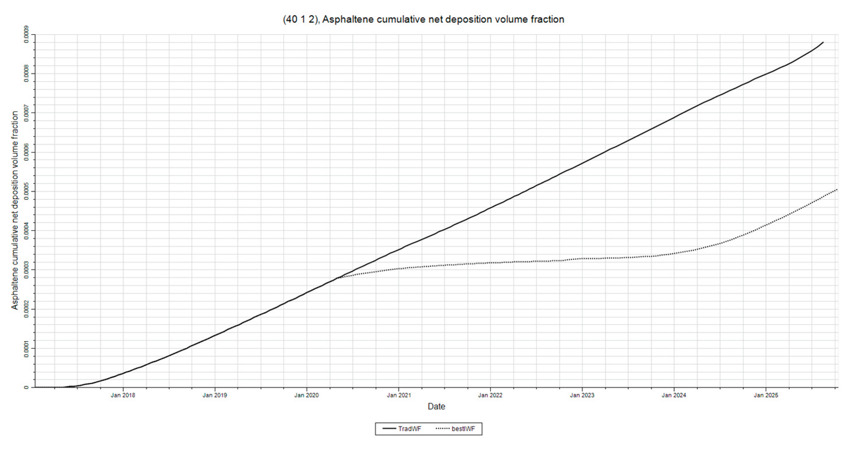
3.4. Comparison of Traditional W.F. to I.W.F. Effects on Asphaltene Damage
Figure 28 illustrates how the processes of the intermittent waterflood differs from that of the traditional waterflood. The intermittent waterflood is conducted in the same manner as it was throughout the study. The intermittent waterflood is optimized for this simulation using the preferred operational parameters determined from the previous sensitivity analyses. The maximum BHP of the injector for the traditional waterflood is set to 2000psi. This BHP limit is set to this value in order to provide a pressure maintenance and displacement mechanism. Once again, each simulation was conducted to produce the same amount of oil so that the amount of hydrocarbons withdrawn from the reservoir do not effect results. The focus of this study was to compare the re-pressurization effects of an intermittent waterflood to the pressure maintenance and displacement mechanism of a traditional waterflood.
Figure 29, Figure 30 and Figure 31 illustrate how the re-pressurization mechanism of intermittent waterflooding can be a better method to mitigate asphaltene deposition when compared to that of traditional waterflooding’s pressure maintenance and displacement mechanism. Asphaltene deposition is shown to be much lower in the intermittent waterflood. This can be explained by the same reasoning from section 3.3.1 where it is stated that intermittent waterflooding introduces a re-stabilization period for system.
4. Conclusions
This study has further expanded upon the observation made by Clavijo14 that intermittent waterflooding can be used to mitigate asphaltene deposition. The mitigation effects can be most clearly observed in the comparison case of section 3.4. The results of this study indicate that:
The time interval between the end of injection and the next production period should be kept to a minimum. Asphaltene deposition should not change over excessive amounts of time. However, minimal increases in asphaltene deposition may be observed as the system approaches equilibrium. These changes are negligible, thus giving reason to reopen the production well as soon as possible to benefit economic feasibility.
The 2015 version of Eclipse 300 simulator appears to have an issue bringing a reservoir system into equilibrium once the pressure is raised and the system is completely close to flow. This issue has been reported to the developers at Stumberger. The utilization of the “SOLIDIMS” keyword could correct this error.
Asphaltene behaviors prominent at distances closer to the producer. This can be explained by effects of pressure drawdown and fluid flow.
Higher injection rates are preferred over lower rates in order to minimize deposition near the producer. Injecting at higher rates also decreases injection time, which can benefit economic feasibility.
Early injection times seem to have a positive impact on asphaltene mitigation. Earlier injection times seemingly “break” trend of increasing rate of deposition and re-stabilize the reservoir more effectively.
References
- Arunagiri, A. T., Gnanasundaram, N., Wilfred, C. D., Rashid, Z., & Murugesan, T. (2019). A comprehensive review on recent advances in petroleum asphaltene aggregation. Journal of Petroleum Science and Engineering, 176, 249–268. [CrossRef]
- Carrera, M., Zarooni, M., Olayiwola, O., Nguyen, V., & Boukadi, F. (2024). Impacts of asphaltene deposition on oil recovery following a waterflood – a numerical simulation study. Journal of Petroleum & Chemical Engineering, 2(1), 1–8.
- Fahes, M., Abraham, J., & Mehana, M. (2019). The impact of asphaltene deposition on fluid flow in sandstone. Journal of Petroleum Science and Engineering, 174, 676–681. [CrossRef]
- Ghadimi, M., Ghaedi, M., Malayeri, M. R., & Amani, M. J. (2020). A new approach to model asphaltene induced permeability damage with emphasis on pore blocking mechanism. Journal of Petroleum Science and Engineering, 184, 106512. [CrossRef]
- Imqam, A., & Elturki, M. (2022). Experimental investigation of asphaltene deposition and aggregation in ultra-low permeability reservoirs under CO₂ injection. Proceedings of the SPE Canada Energy Technology Conference, SPE-208563-MS.
- Khurshid, I., Al-Attar, H., & Alraeesi, A. R. (2018). Modeling cementation in porous media during waterflooding: Asphaltene deposition, formation dissolution, and their cementation. Journal of Petroleum Science and Engineering, 161, 359–367. [CrossRef]
- Lo, A., Tinni, A., & Milad, B. (2021). Experimental study on the influences of pressure and flow rates in the deposition of asphaltenes in a sandstone core sample. Fuel, 292, 120261. [CrossRef]
- Milad, B., Tinni, O. A., & Lo, A. P. (2022). Experimental study on the influence of flow rate and pressure on the deposition of asphaltenes in a sandstone core sample. Fuel, 310, 122420. [CrossRef]
- Mohebbinia, S., Sepehrnoori, K., Johns, R. T., & Kazemi Nia Korrani, A. (2017). Simulation of asphaltene precipitation during gas injection using PC-SAFT EOS. Journal of Petroleum Science and Engineering, 158, 693–706. [CrossRef]
- Saboor, A., Yousaf, N., Haneef, J., & Ali, S. I. (2022). Performance of asphaltene stability predicting models in field environment and development of a new predictor. Journal of Petroleum Exploration and Production Technology, 12(4), 1423–1436. [CrossRef]
- Shekarifard, A., Shakib-Taheri, J., & Naderi, H. (2018). Experimental investigation of asphaltene deposition in porous media under ultrasonic and microwave fields. Journal of Petroleum Science and Engineering, 163, 453–462. [CrossRef]
- Xiong, R., Guo, J., Kiyingi, W., & Li, Q. (2020). Method for judging the stability of asphaltenes in crude oil. ACS Omega, 5(36), 23131–23140. [CrossRef]
- Yin, D., Li, Q., & Zhao, D. (2023). Investigating asphaltene precipitation and deposition in ultra-low permeability reservoirs during CO₂-EOR. Sustainability, 16(10), 4303. [CrossRef]
- Clavijo, J. Intermittent Waterflooding for Asphaltene Mitigation: Laboratory Observations. 2011. (Data set and observations used for model calibration in this study.
- Xiong, R., Guo, J., Kiyingi, W., Xu, H., and Wu, X. “The Deposition of Asphaltenes under High-Temperature and High-Pressure (HTHP) Conditions.” Petroleum Science, vol. 20, 2023, pp. 611–618. [CrossRef]
- Tahernejad, E., Bazvand, M., and Shadizadeh, S. R. “Asphaltene Deposition Effects on Reservoir Rock Wettability and Permeability: An Experimental Study.” Scientific Reports, vol. 14, 2024, article no. 15249. [CrossRef]
- Alemi, F. M., and Mohammadi, S. “Experimental Study on Water-in-Oil Emulsion Stability Induced by Asphaltene Colloids in Heavy Oil.” ACS Omega, 2025. [CrossRef]
- Wang, S., and F. Civan. “Preventing Asphaltene Deposition in Oil Reservoirs by Early Water Injection.” SPE Production Operations Symposium, Society of Petroleum Engineers, 2005, Paper SPE-94268.
- Ali, S. I., Lalji, S. M., Haneef, J., Tariq, S. M., Junaid, M., & Ali, S. M. A. (2022). Determination of asphaltene stability in crude oils using a deposit level test coupled with a spot test: A simple and qualitative approach. ACS Omega, 7(16), 14165–14179. [CrossRef]
- Stratiev, D., Nikolova, R., Veli, A., Shishkova, I., Toteva, V., & Georgiev, G. (2025). Mitigation of asphaltene deposit formation via chemical additives: A review. Processes, 13(1), 141. [CrossRef]
- Choiri, M., and Hamouda, A.A. (2011). Enhanced Oil Recovery by CO2 Flooding Effect on Asphaltene Stability Envelope and Compositional Simulation of Asphaltenic Oil Reservoir. SPE 141329.
- Isah, M., Mahmoud, M., Al-Shehri, D., Alade, L., et. (2020). Asphaltene precipitation and deposition: A critical review. Journal of Petroleum Science and Engineering, *197*, 107956. [CrossRef]
Figure 2.
Reservoir Interaction. This figure illustrates various processes and behaviors in the reservoir for the entirety of the study.
Figure 2.
Reservoir Interaction. This figure illustrates various processes and behaviors in the reservoir for the entirety of the study.
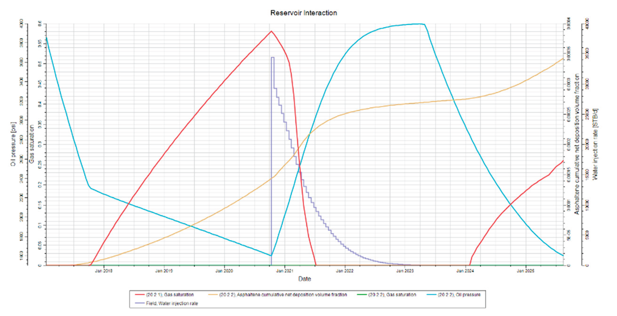
Figure 3.
Reservoir Shut-in Sensitivity. This figure illustrates the time shut-in time parameter that is varied for this sensitivity analysis.
Figure 3.
Reservoir Shut-in Sensitivity. This figure illustrates the time shut-in time parameter that is varied for this sensitivity analysis.
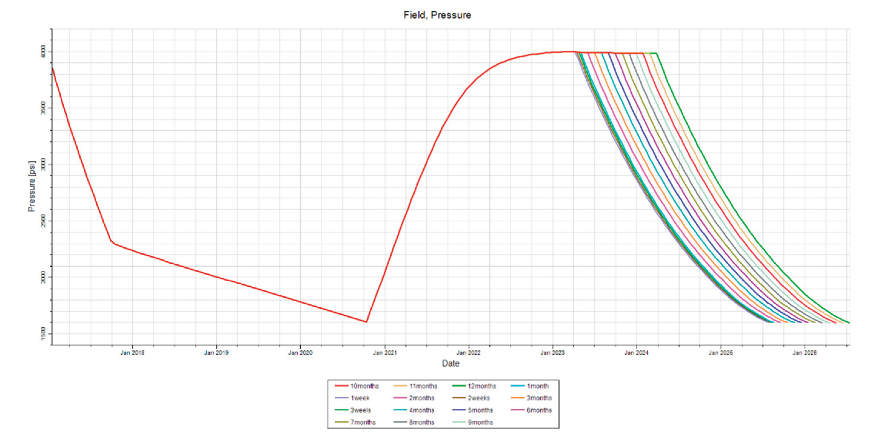
Figure 4.
Deposition by Injector. This figure shows the asphaltene deposition at the injector in layers 1-4 for the shut-in time sensitivity analysis.
Figure 4.
Deposition by Injector. This figure shows the asphaltene deposition at the injector in layers 1-4 for the shut-in time sensitivity analysis.
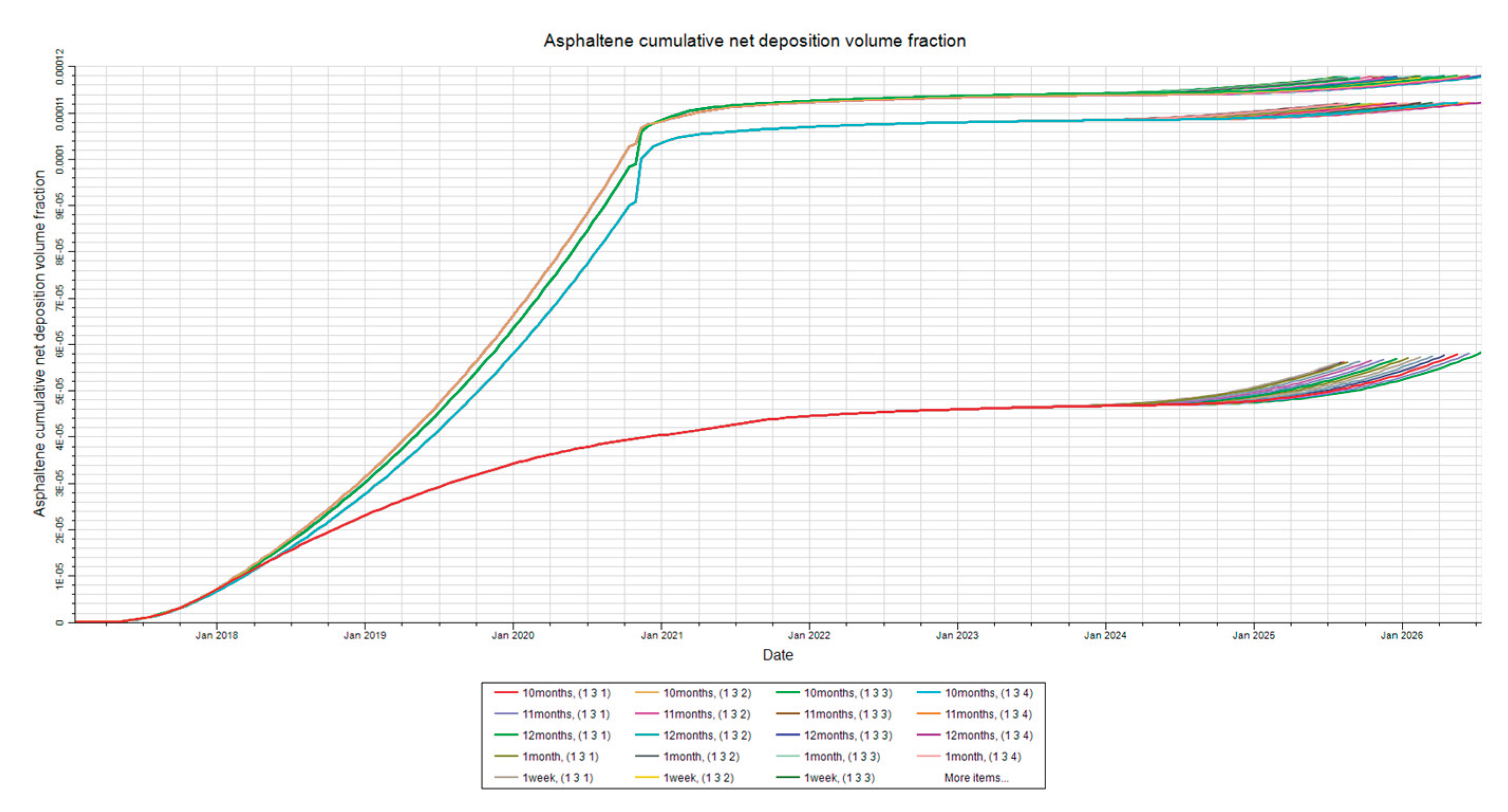
Figure 5.
Deposition at Mid-Point. This figure shows the asphaltene deposition at the mid-point in layers 1-4 for the shut-in time sensitivity analysis.
Figure 5.
Deposition at Mid-Point. This figure shows the asphaltene deposition at the mid-point in layers 1-4 for the shut-in time sensitivity analysis.
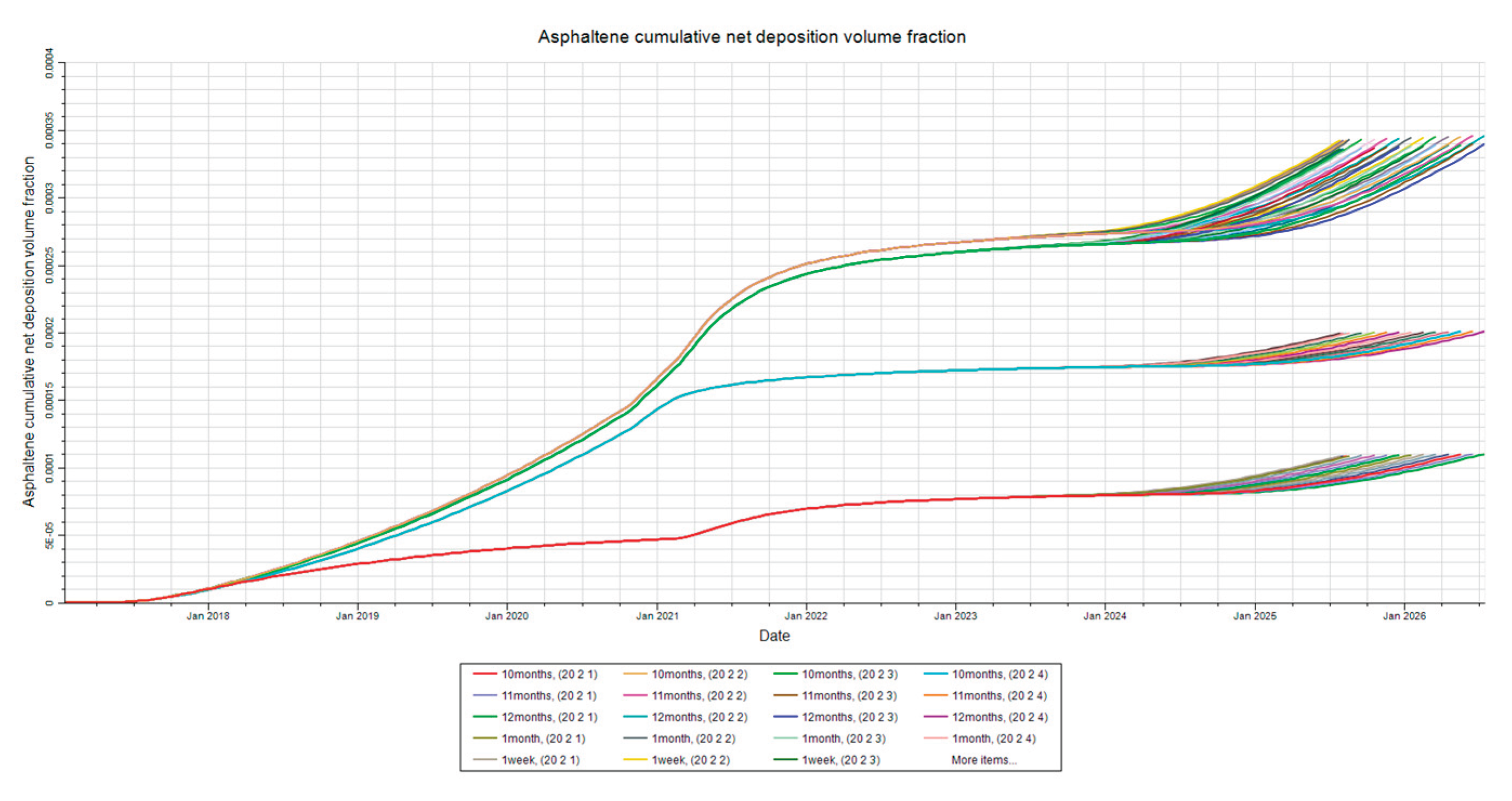
Figure 6.
Deposition at Producer. This figure shows the asphaltene deposition at the producer in layers 1-4 for the shut-in time sensitivity analysis.
Figure 6.
Deposition at Producer. This figure shows the asphaltene deposition at the producer in layers 1-4 for the shut-in time sensitivity analysis.
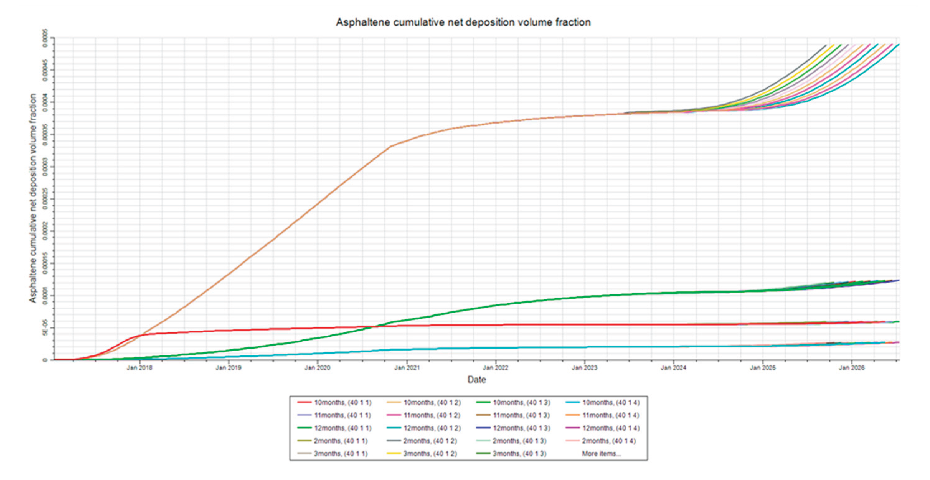
Figure 7.
Permeability Damage at Injector. This figure shows the permeability damage, quantified as a multiplier, due to asphaltene deposition at the injector in layers 1-4 for the shut-in time sensitivity analysis.
Figure 7.
Permeability Damage at Injector. This figure shows the permeability damage, quantified as a multiplier, due to asphaltene deposition at the injector in layers 1-4 for the shut-in time sensitivity analysis.
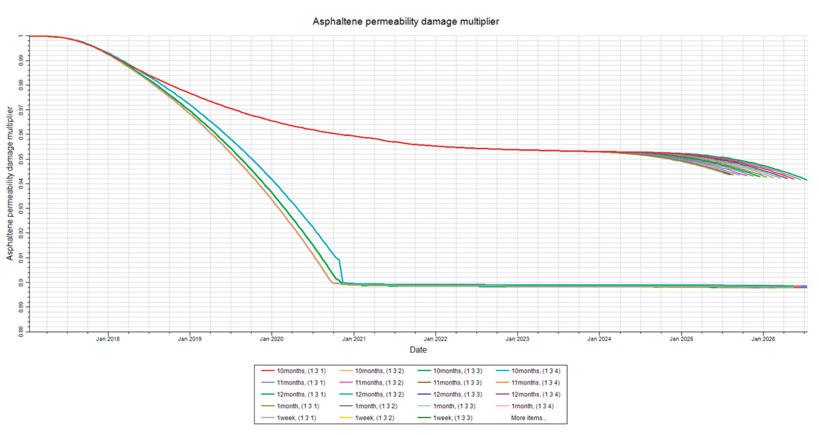
Figure 8.
Permeability Damage at Mid-Point. This figure shows the permeability damage, quantified as a multiplier, due to asphaltene deposition at the mid-point in layers 1-4 for the shut-in time sensitivity analysis.
Figure 8.
Permeability Damage at Mid-Point. This figure shows the permeability damage, quantified as a multiplier, due to asphaltene deposition at the mid-point in layers 1-4 for the shut-in time sensitivity analysis.
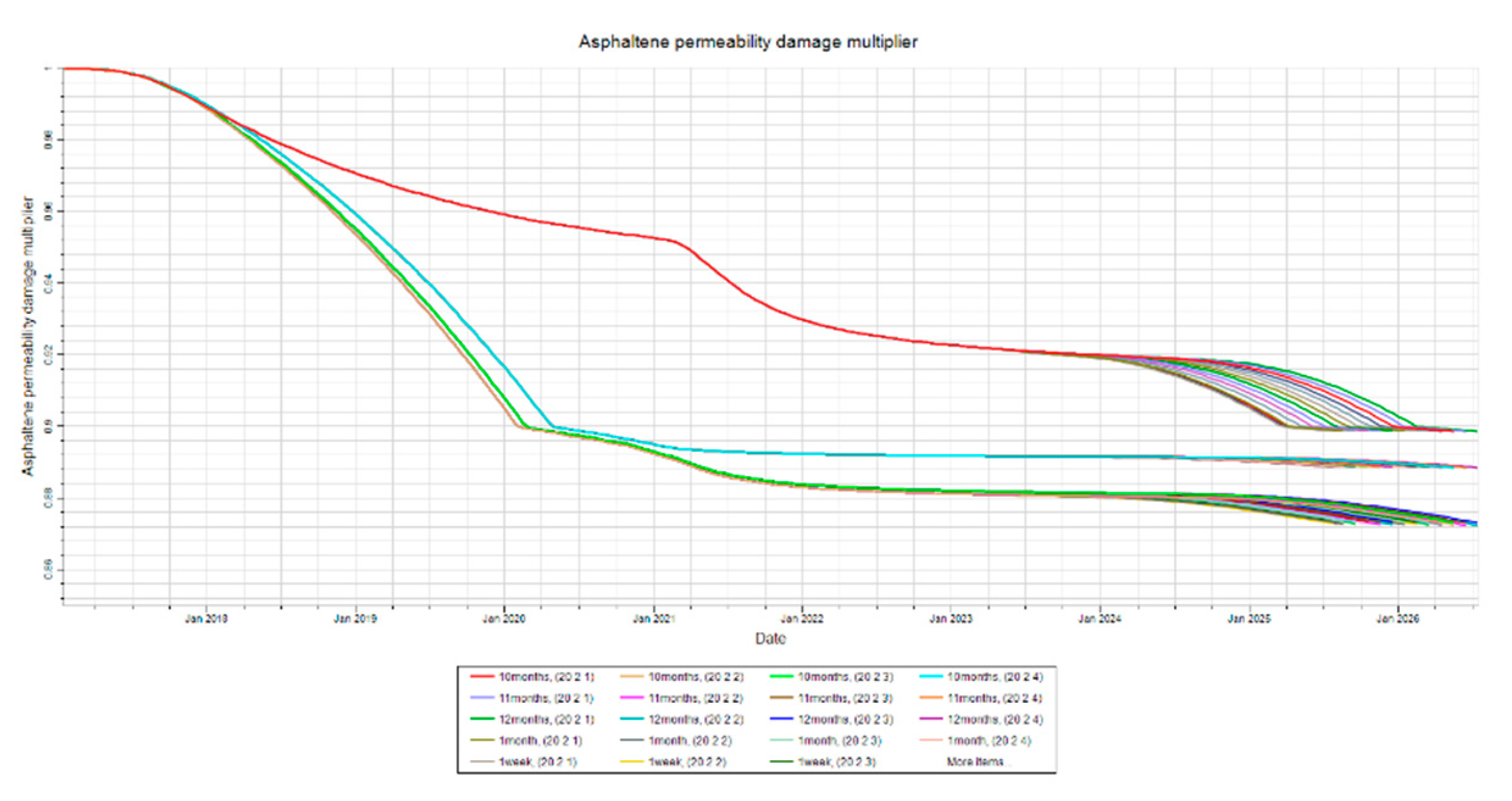
Figure 9.
Permeability Damage at Producer. This figure shows the permeability damage, quantified as a multiplier, due to asphaltene deposition at the producer in layers 1-4 for the shut-in time sensitivity analysis.
Figure 9.
Permeability Damage at Producer. This figure shows the permeability damage, quantified as a multiplier, due to asphaltene deposition at the producer in layers 1-4 for the shut-in time sensitivity analysis.
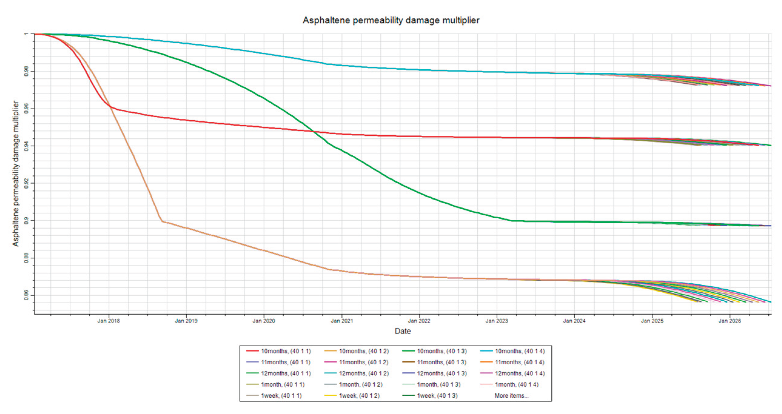
Figure 10.
Plugging at Injector. This figure shows the volume fraction of the asphaltene that is responsible for plugging pore throats in layers 1-4 for the shut-in time sensitivity analysis.
Figure 10.
Plugging at Injector. This figure shows the volume fraction of the asphaltene that is responsible for plugging pore throats in layers 1-4 for the shut-in time sensitivity analysis.
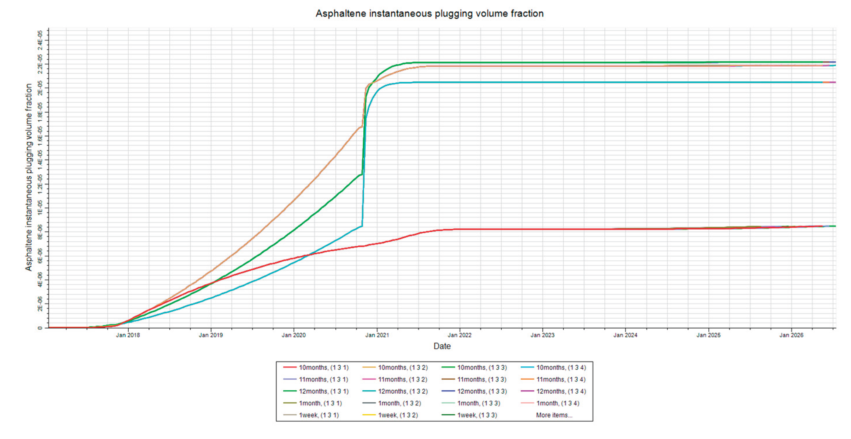
Figure 11.
Plugging at Mid-Point. This figure shows the volume fraction of the asphaltene that is responsible for plugging pore throats in layers 1-4 for the shut-in time sensitivity analysis.
Figure 11.
Plugging at Mid-Point. This figure shows the volume fraction of the asphaltene that is responsible for plugging pore throats in layers 1-4 for the shut-in time sensitivity analysis.
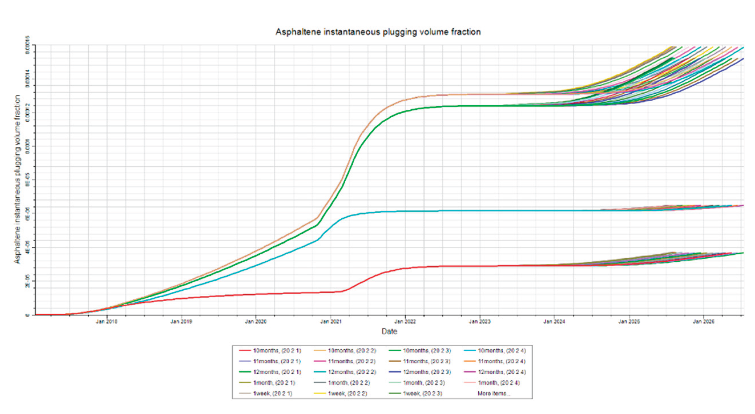
Figure 12.
Plugging at Producer. This figure shows the volume fraction of the asphaltene that is responsible for plugging pore throats in layers 1-4 for the shut-in time sensitivity analysis.
Figure 12.
Plugging at Producer. This figure shows the volume fraction of the asphaltene that is responsible for plugging pore throats in layers 1-4 for the shut-in time sensitivity analysis.
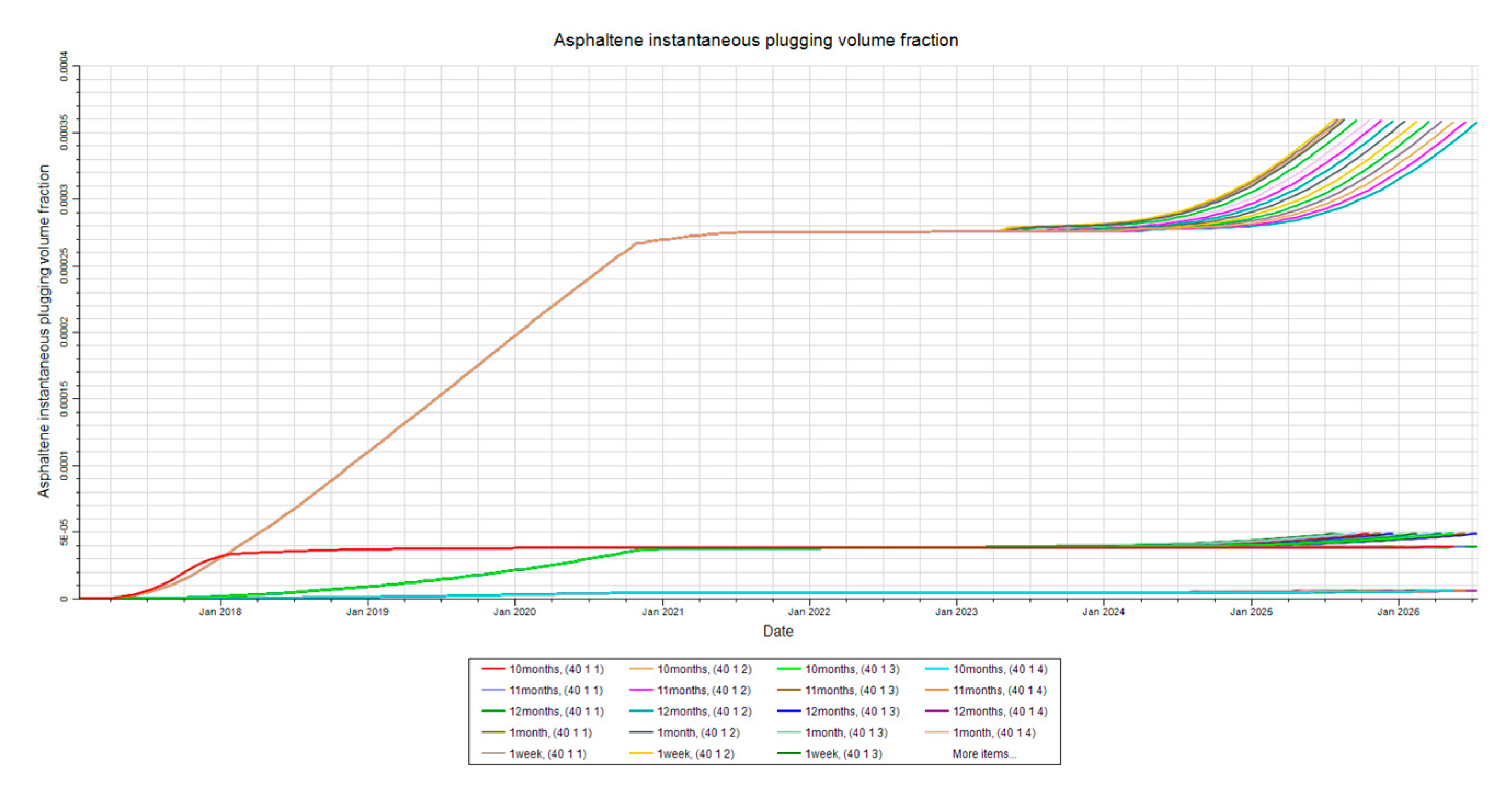
Figure 13.
Deposition at Producer, Mid-Point. This figure shows the asphaltene deposition in layer two at all three locations of inspection for the shut-in time sensitivity analysis.
Figure 13.
Deposition at Producer, Mid-Point. This figure shows the asphaltene deposition in layer two at all three locations of inspection for the shut-in time sensitivity analysis.
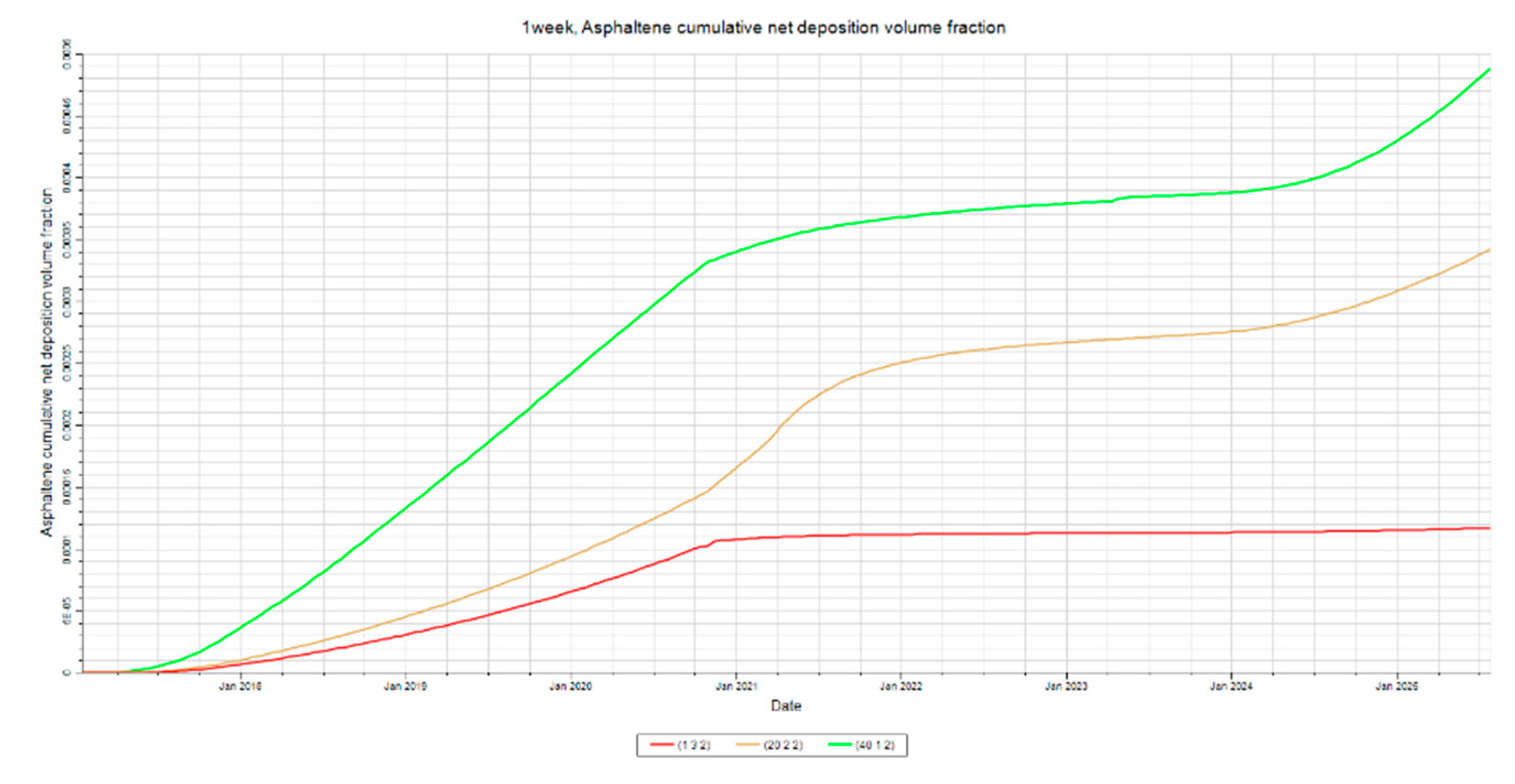
Figure 14.
Permeability Damage at Injector, Mid-Point and Producer. This figure shows the permeability damage in layer two at all three locations of inspection for the shut-in time sensitivity analysis.
Figure 14.
Permeability Damage at Injector, Mid-Point and Producer. This figure shows the permeability damage in layer two at all three locations of inspection for the shut-in time sensitivity analysis.
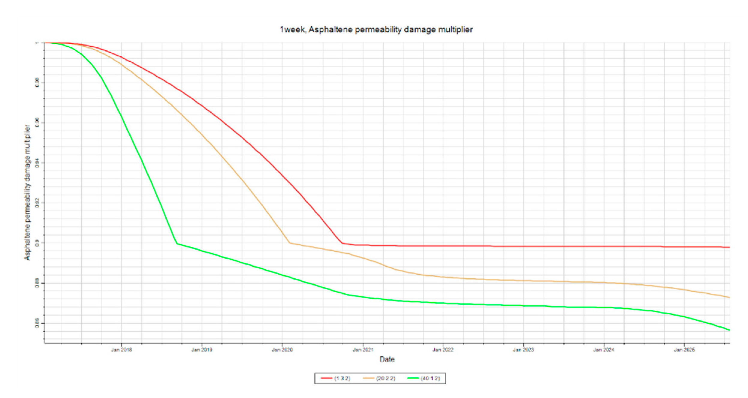
Figure 15.
Plugging at Injector, Mid-Point and producer. This figure shows the asphaltene volume responsible for plugging pore throats in layer two at all three locations of inspection for the shut-in time sensitivity analysis.
Figure 15.
Plugging at Injector, Mid-Point and producer. This figure shows the asphaltene volume responsible for plugging pore throats in layer two at all three locations of inspection for the shut-in time sensitivity analysis.
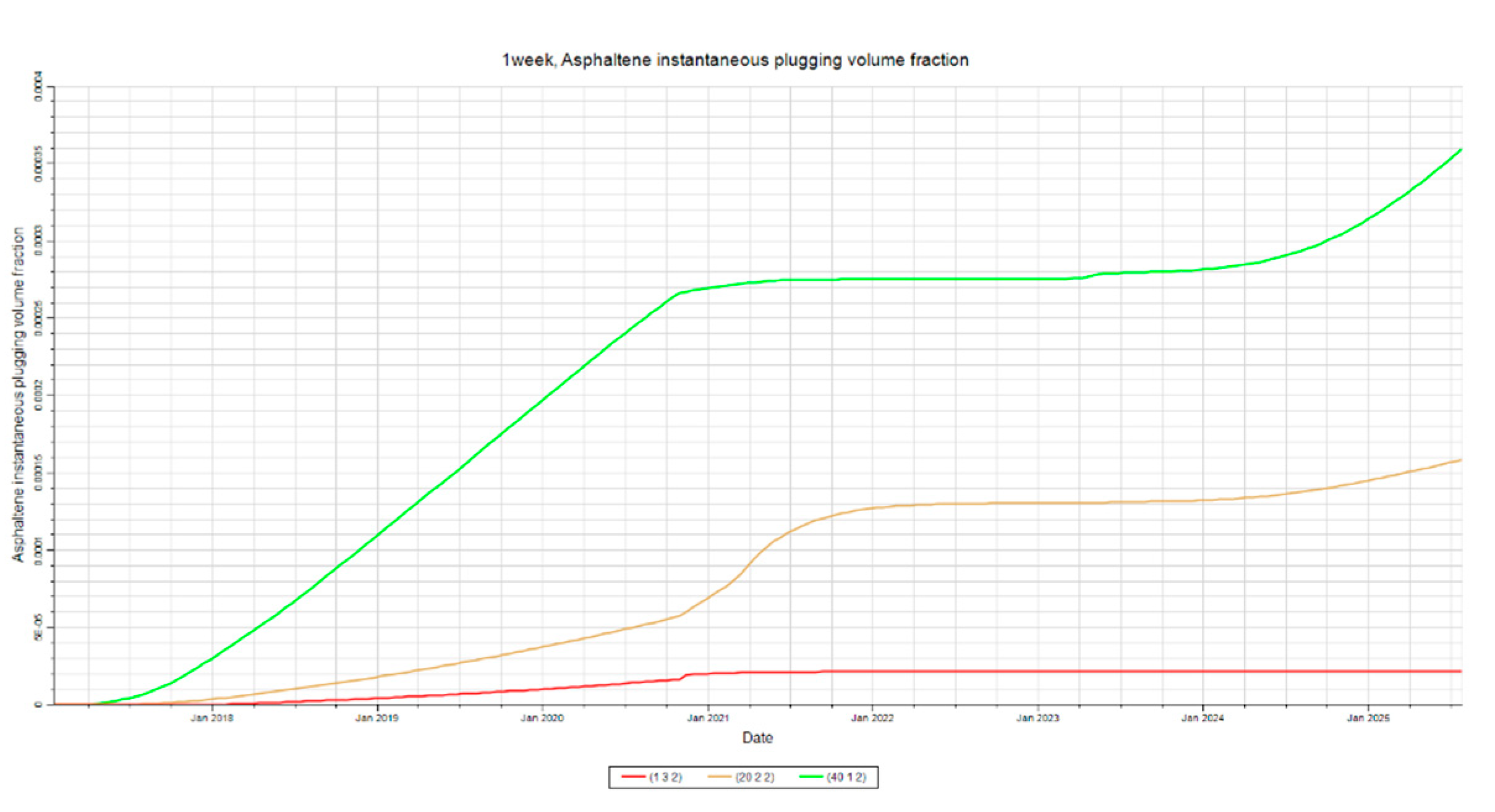
Figure 16.
Streamlines During Production. This figure illustrates the streamlines at a point in time during production in order to highlight the convergence at the producer.
Figure 16.
Streamlines During Production. This figure illustrates the streamlines at a point in time during production in order to highlight the convergence at the producer.
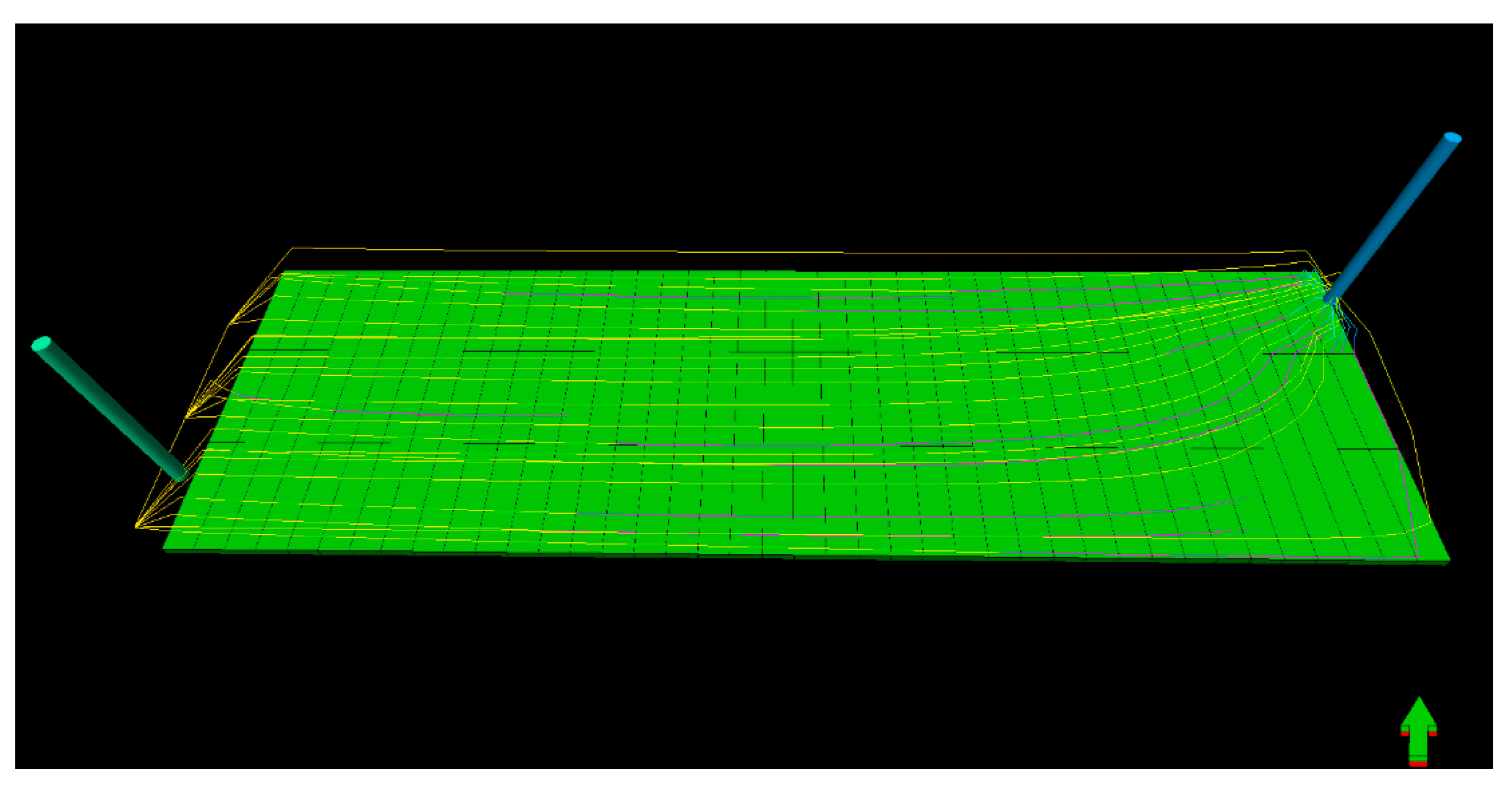
Figure 17.
Injection Rate Variance. This figure illustrates how the injection rate is varied for this sensitivity analysis.
Figure 17.
Injection Rate Variance. This figure illustrates how the injection rate is varied for this sensitivity analysis.
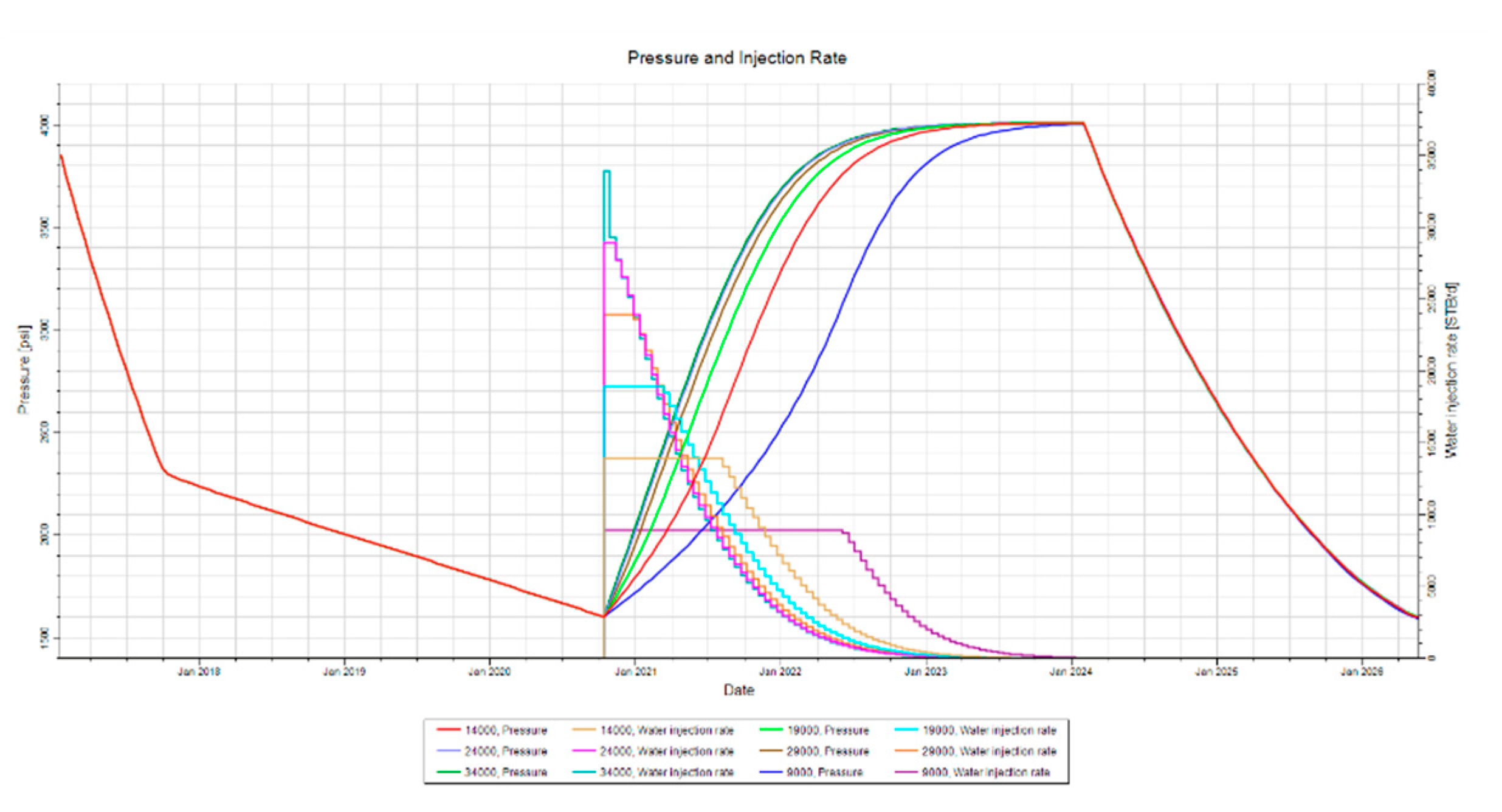
Figure 18.
Deposition at Injector. This figure shows the asphaltene deposition at the injector in layer 2 for the injection rate sensitivity analysis.
Figure 18.
Deposition at Injector. This figure shows the asphaltene deposition at the injector in layer 2 for the injection rate sensitivity analysis.

Figure 19.
Deposition at Mid-Point. This figure shows the asphaltene deposition at the mid-point in layer 2 for the injection rate sensitivity analysis.
Figure 19.
Deposition at Mid-Point. This figure shows the asphaltene deposition at the mid-point in layer 2 for the injection rate sensitivity analysis.
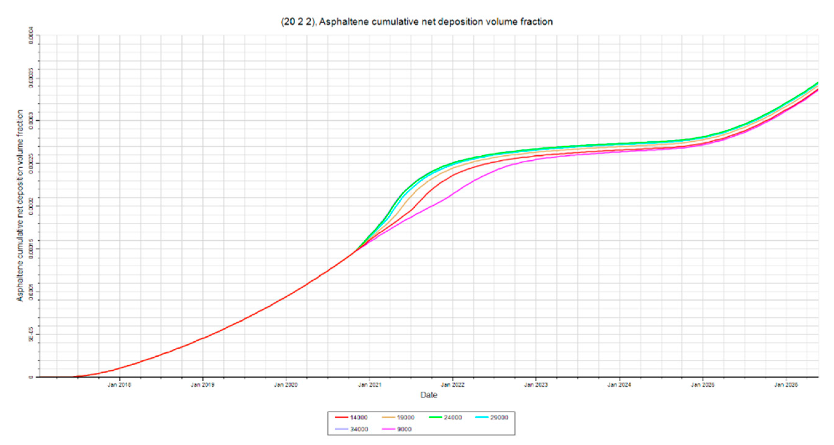
Figure 20.
Deposition at Producer. This figure shows the asphaltene deposition at the producer in layer 2 for the injection rate sensitivity analysis.
Figure 20.
Deposition at Producer. This figure shows the asphaltene deposition at the producer in layer 2 for the injection rate sensitivity analysis.
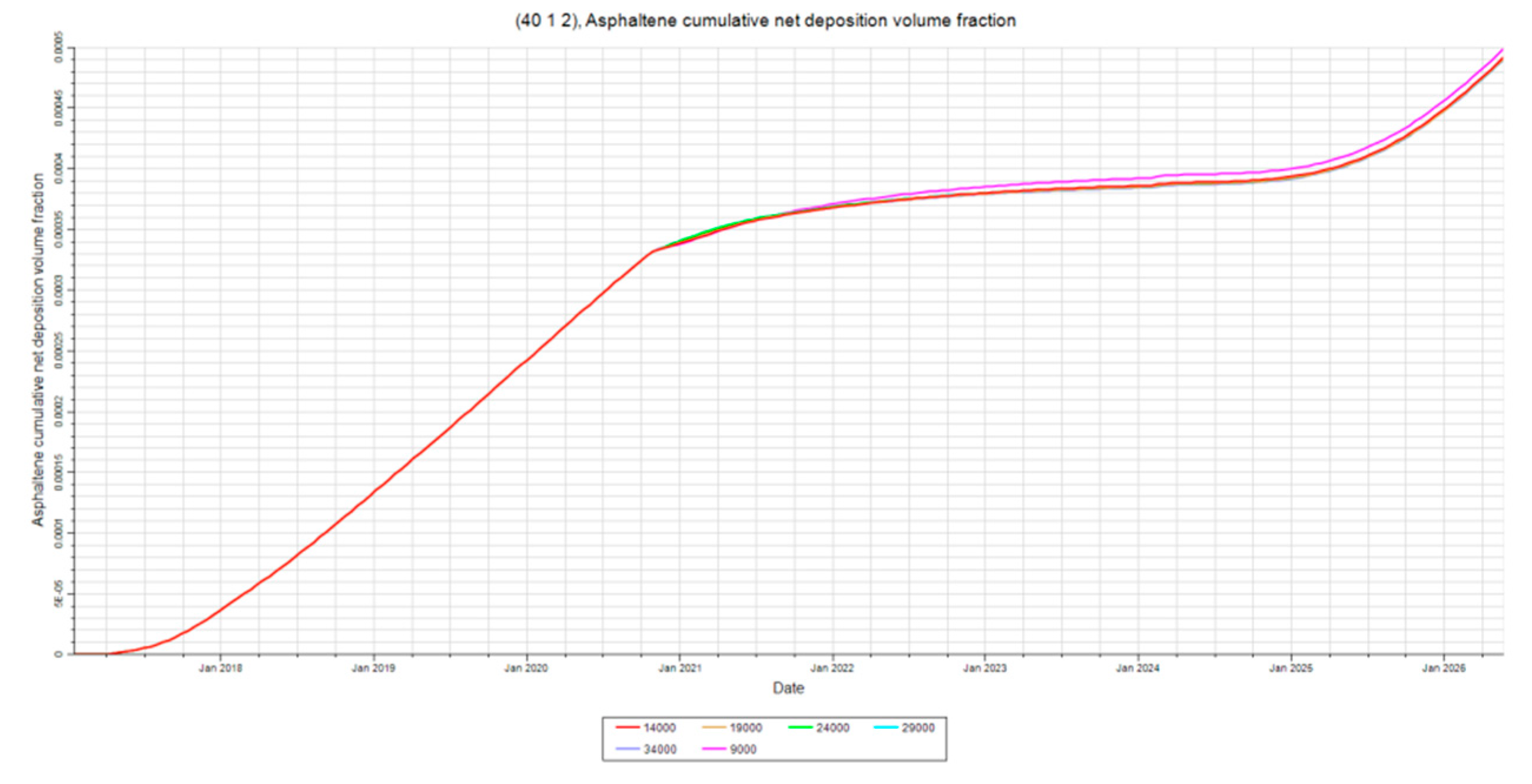
Figure 21.
Deposition, Permeability, and Plugging at Injector. This figure shows all three outputs evaluated for this study at the injector in layer 2.
Figure 21.
Deposition, Permeability, and Plugging at Injector. This figure shows all three outputs evaluated for this study at the injector in layer 2.

Figure 22.
Deposition, Permeability, and Plugging at Mid-Point. This figure shows all three outputs evaluated for this study at the mid-point in layer 2.
Figure 22.
Deposition, Permeability, and Plugging at Mid-Point. This figure shows all three outputs evaluated for this study at the mid-point in layer 2.
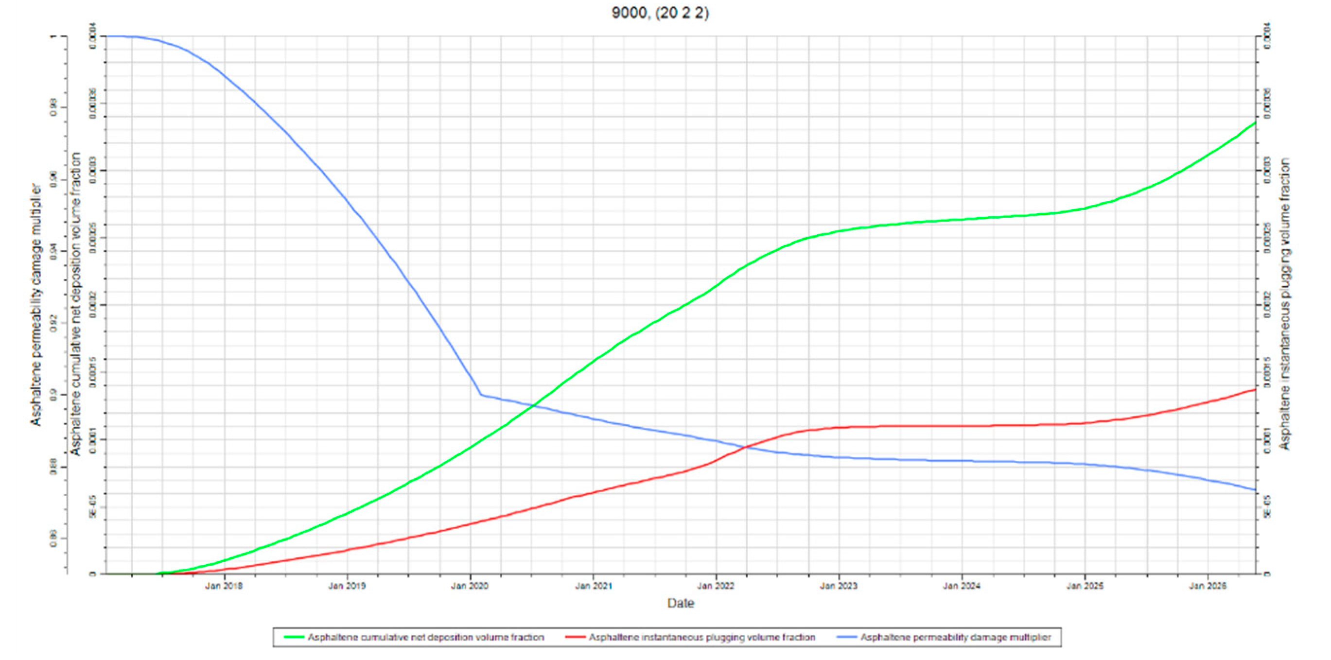
Figure 23.
Deposition, Permeability, and Plugging at Producer. This figure shows all three outputs evaluated for this study at the producer in layer 2.
Figure 23.
Deposition, Permeability, and Plugging at Producer. This figure shows all three outputs evaluated for this study at the producer in layer 2.
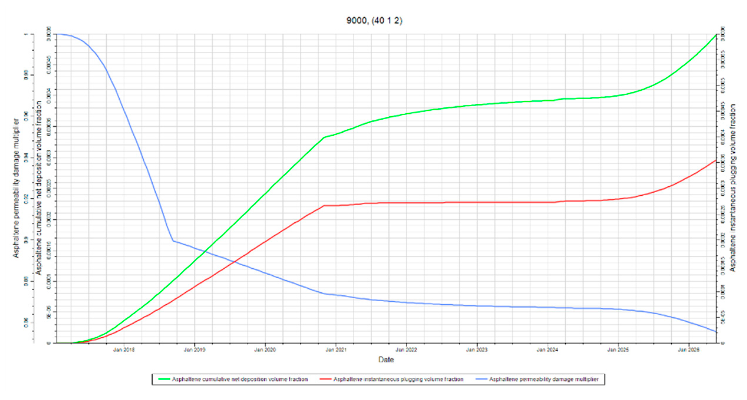
Figure 24.
Time of Injection Sensitivity. This figure illustrates how the injection time was varied for this analysis while keeping the cumulative produced oil constant.
Figure 24.
Time of Injection Sensitivity. This figure illustrates how the injection time was varied for this analysis while keeping the cumulative produced oil constant.
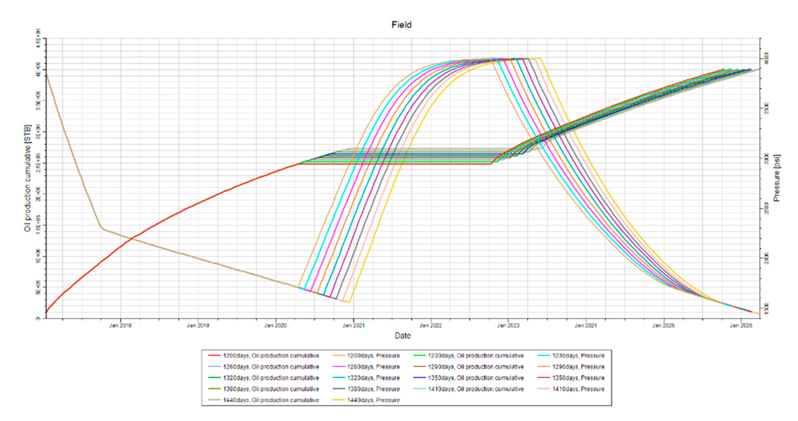
Figure 25.
Asphaltene Deposition at Injector. This figure shows the asphaltene deposition at the injector in layer two for the injection time sensitivity analysis.
Figure 25.
Asphaltene Deposition at Injector. This figure shows the asphaltene deposition at the injector in layer two for the injection time sensitivity analysis.
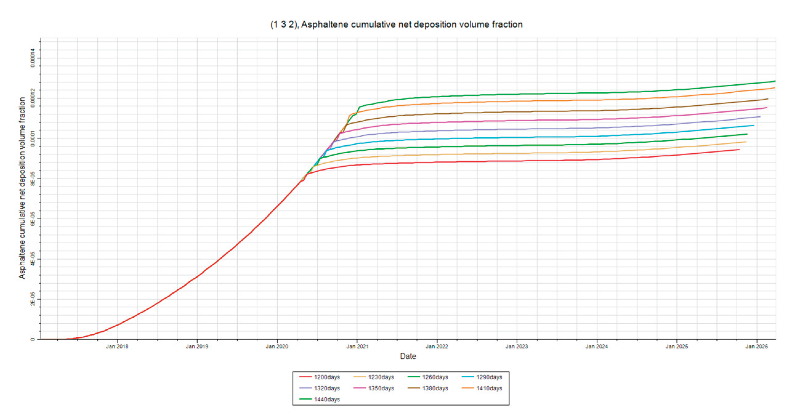
Figure 26.
Asphaltene Deposition at Mid-Point. This figure shows the asphaltene deposition at the mid-point in layer two for the injection time sensitivity analysis.
Figure 26.
Asphaltene Deposition at Mid-Point. This figure shows the asphaltene deposition at the mid-point in layer two for the injection time sensitivity analysis.
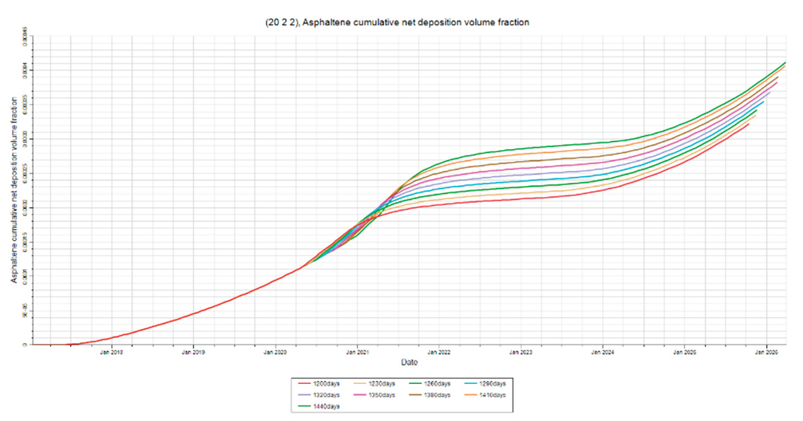
Figure 27.
Asphaltene Deposition at Producer. This figure shows the asphaltene deposition at the producer in layer two for the injection time sensitivity analysis.
Figure 27.
Asphaltene Deposition at Producer. This figure shows the asphaltene deposition at the producer in layer two for the injection time sensitivity analysis.
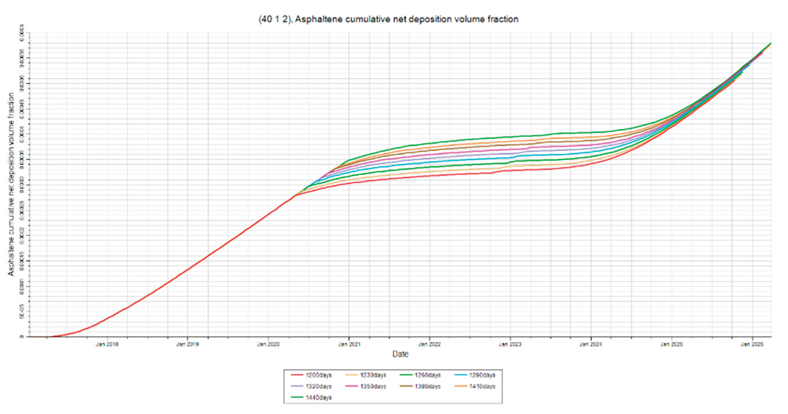
Figure 28.
Intermittent vs Traditional Waterflood Pressure and Production. This figure highlights the differences between a traditional waterflood and an intermittent waterflood.
Figure 28.
Intermittent vs Traditional Waterflood Pressure and Production. This figure highlights the differences between a traditional waterflood and an intermittent waterflood.
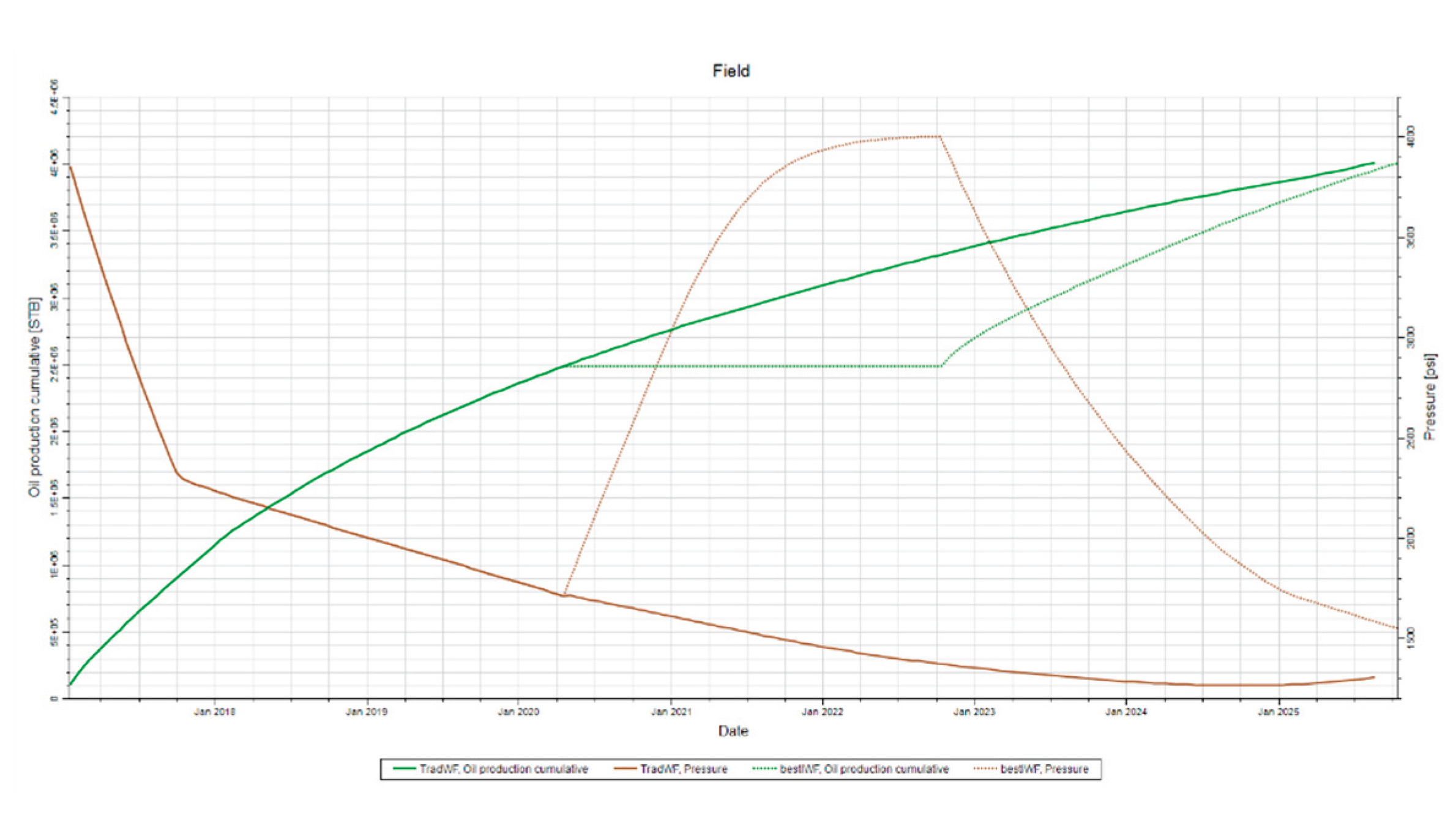
Figure 29.
I.W.F. vs Traditional Waterflood Asphaltene Deposition at Injector. This figure shows how I.W.F. can reduce asphaltene deposition at the injector.
Figure 29.
I.W.F. vs Traditional Waterflood Asphaltene Deposition at Injector. This figure shows how I.W.F. can reduce asphaltene deposition at the injector.
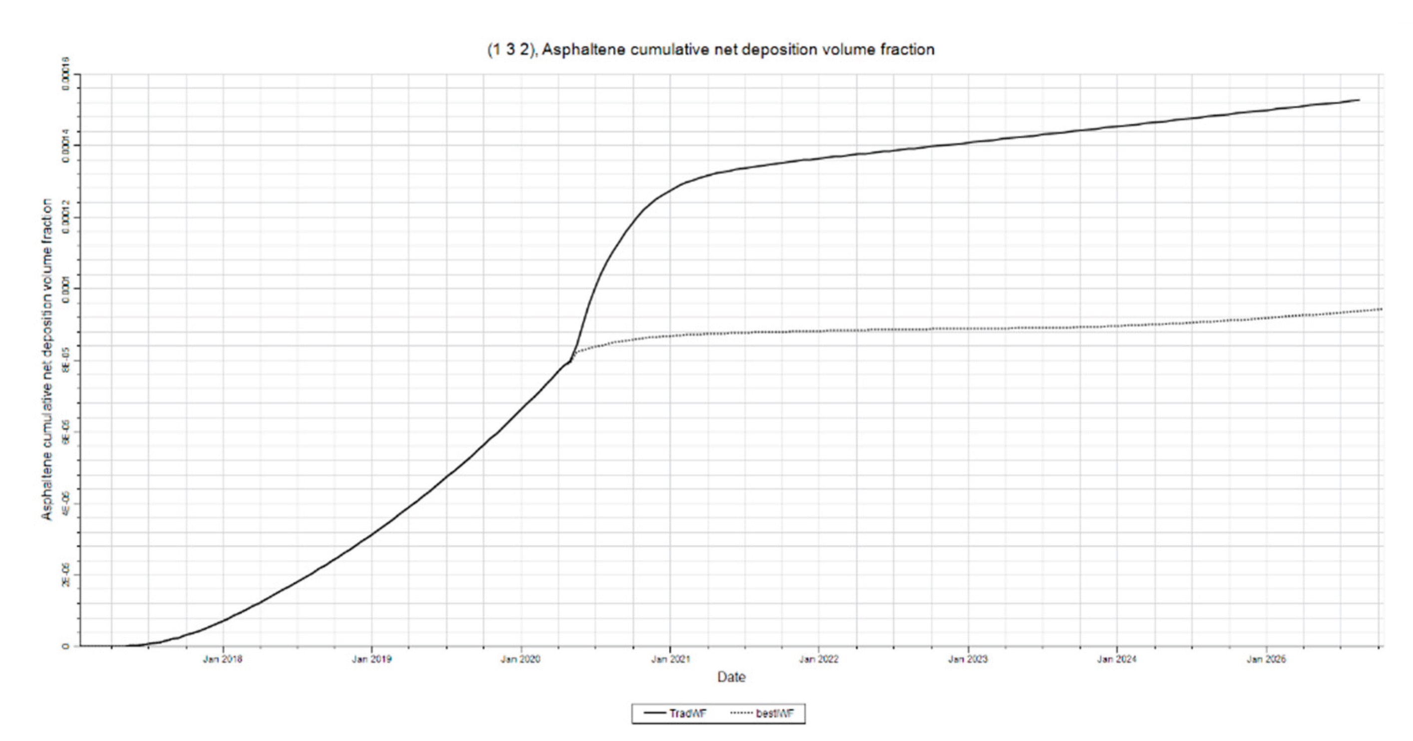
Figure 30.
I.W.F. vs Traditional Waterflood Asphaltene Deposition at Mid-Point. This figure shows how I.W.F. can reduce asphaltene deposition at the mid-point.
Figure 30.
I.W.F. vs Traditional Waterflood Asphaltene Deposition at Mid-Point. This figure shows how I.W.F. can reduce asphaltene deposition at the mid-point.

Figure 31.
I.W.F. vs Traditional Waterflood Asphaltene Deposition at Producer. This figure shows how I.W.F. can reduce asphaltene deposition at the producer.
Figure 31.
I.W.F. vs Traditional Waterflood Asphaltene Deposition at Producer. This figure shows how I.W.F. can reduce asphaltene deposition at the producer.
Disclaimer/Publisher’s Note: The statements, opinions and data contained in all publications are solely those of the individual author(s) and contributor(s) and not of MDPI and/or the editor(s). MDPI and/or the editor(s) disclaim responsibility for any injury to people or property resulting from any ideas, methods, instructions or products referred to in the content. |
© 2025 by the authors. Licensee MDPI, Basel, Switzerland. This article is an open access article distributed under the terms and conditions of the Creative Commons Attribution (CC BY) license (http://creativecommons.org/licenses/by/4.0/).
Copyright: This open access article is published under a Creative Commons CC BY 4.0 license, which permit the free download, distribution, and reuse, provided that the author and preprint are cited in any reuse.


