Submitted:
20 May 2025
Posted:
20 May 2025
You are already at the latest version
Abstract
Ice thickness is a key parameter for glacier mass estimations and glacier dynamics simulations. Multiple physical models have been developed by glaciologists to estimate glacier ice thickness. However, obtaining internal and basal glacier parameters required by physical models is challenging, often leading to simplified models that struggled to capture the nonlinear characteristics of ice flow and resulting in significant uncertainties. To address this, this study proposes a convolutional neural network (CNN) -based deep learning model for glacier ice thickness estimation, named the Coordinate-Attentive Dense Glacier Ice Thickness Estimate Model (CADGITE). Based on in situ ice thickness measurements in the Swiss Alps, a CNN is designed to estimate glacier ice thickness by incorporating a new architecture that includes Residual Coordinate Attention Block together with Dense Connected Block, using distance to glacier boundaries as a complement of inputs that include surface velocity, slope, and hypsometry. Taking ground-penetrating radar (GPR) measurements as reference, the proposed model achieves a mean absolute deviation (MAD) of 24.61 m and a root mean square error (RMSE) of 39.09 m in Switzerland, outperforming mainstream physical models. When applied to 14 glaciers in High Mountain Asia, the model achieves an MAD of 20.38 m and an RMSE of 26.14 m compared to reference measurements, also exhibiting better performance than mainstream physical models. These comparisons demonstrate the good accuracy and cross-regional transferability of our approach, highlighting the potential of using deep-learning-based methods for larger-scale glacier ice thickness estimation.
Keywords:
glacier ice thickness
; deep learning
; CNN
; Swiss
; High Mountain Asia
1. Introduction
Ice thickness data are crucial for estimating glacier mass storage, as well as constraining glacier basal topography and ice deformation in dynamic models [1]. Traditional methods such as ground drilling and GPR can provide accurate point measurements, but their high cost and low efficiency limit large-scale application. By combining surface remote sensing observations and digital elevation models, glacier ice thickness can be estimated through physical models. The Ice Thickness Models Intercomparison eXperiment (ITMIX) compared 17 glacier ice thickness estimation methods and revealed significant differences among the results [2]. These models can be mainly categorized into: 1) minimization approaches [3,4]: constructing forward ice flow models to simulate observable quantities, in which model parameters are iteratively optimized to infer ice thickness by minimizing a cost function that quantifies the mismatch between observations and simulations; 2) mass-conserving approaches [5,6,7]: using estimates of surface mass balance and elevation change rates to calculate ice fluxes, from which ice thickness can be derived; 3) shear-stress-based approaches [8,9,10]: assuming a constant basal shear stress across the glacier and apply the Shallow Ice Approximation to estimate ice thickness; 4) velocity-based approaches [11,12]: employing Glen’s flow law to directly compute ice thickness by using surface velocity and slope as key inputs. To estimate ice thickness over the entire glacier, some methods also incorporate spatial interpolation techniques to extrapolate localized results across the full glacier extent. However, due to the scarcity of direct observations beneath and within glaciers, all these models introduce varying degrees of simplification during their development, such as linear approximations of ice flow dynamics and empirically derived parameters. These simplifications and assumptions are major sources of model uncertainty, making current models struggle to fully capture the nonlinear dynamics of ice flow, which in turn limits the overall accuracy and applicability for ice thickness estimation.
Deep learning methods can integrate multi-source remote sensing data, glacier topographic information, and in situ GPR measurements to automatically learn complex nonlinear relationships between glacier ice thickness and its influencing factors, leveraging their strong feature extraction and pattern recognition capabilities. Several studies have explored the use of neural networks for glacier ice thickness estimation and subglacial topography reconstruction. In 2009, Clark et al. assumed that ice-free areas surrounding glaciers were formerly ice-covered and used the terrain data of these areas to train an artificial neural network (ANN) for glacier ice thickness prediction [13]. In 2020, Wei Ji et al. developed a generative adversarial network (GAN) integrating multi-source data for super-resolution reconstruction of Antarctic subglacial topography [14]. Haq et al. (2021) combined DEM data and ANN to estimate the ice thickness of the Chhota Shigri Glacier [15]. Lopez Uroz et al. (2024) combined convolutional networks with multi-source data to simulate glacier ice thickness in Switzerland [16]. Monnier and Zhu (2021), as well as Steidl et al. (2025), used physics-informed artificial neural networks (ANNs) for subglacial topography reconstruction and glacier ice thickness estimation [17,18]. These data-driven methods can, to some extent, capture nonlinear ice flow features that physical models fail to represent. When sufficient data are available, data-driven methods can achieve higher accuracy than physical models.
However, existing deep learning-based methods for glacier ice thickness estimation continue to face challenges in effectively extracting multi-scale spatial features, and network architecture that could potentially influence the accuracy of thickness estimations still needs further optimization. In details, ice thickness shows varying sensitivity to different input glacier characteristics, making it crucial to accurately learn the weight of different semantic information in thickness estimation. Furthermore, the selected model needs to be capable to capture the distinct spatial distribution characteristics of different input features. Currently, a variety of structural modules such as attention mechanisms [19,20] have been developed to enhance feature representation capabilities, offering diverse components and strategies for network architecture design. Moreover, the input glacier features are limited. Although surface velocity, slope, and elevation data are commonly used, other important features related to glacier ice thickness have not yet been incorporated into model training. For example, glacier ice thickness tends to increase with distance from the glacier boundary, and valley glacier cross-sections are often “U” shaped, such geometric characteristic shows significant correlations with ice thickness. Therefore, by improving network architectures and optimizing input features, multi-source data-driven deep learning methods have the potential to produce more accurate and robust glacier ice thickness estimations.
This study develops a multi-branch network architecture that incorporates surface velocity, slope, hypsometry, and newly added distance to the boundary as input features for training. A coordinate attention mechanism is introduced to enhance the spatial feature modeling capability of the deep convolutional neural network. The features from each branch were fused using a dense block that employs cross-layer connections to enhance feature reuse and gradient propagation. This fusion enables the model to capture complex nonlinear interactions among multi-source physical parameters influencing glacier ice thickness. The proposed deep network model (CADGITE) is trained on high-precision glacier ice thickness data from the Swiss Alps and further applied to glaciers in various sub-regions of High Mountain Asia to evaluate its generalization capability and applicability across diverse glacial environments.
2. Study Area and Data
2.1. Overview of Glaciers in Switzerland and High Mountain Asia
Figure 1 illustrates the distribution of glaciers in Switzerland. Glacier boundaries are derived from the Swiss Glacier Inventory 2016 (SGI2016) [21]. This region contains 1,400 glaciers, covering a total area of 961 km². Most glaciers are relatively small, with approximately 82% having an area of less than 0.5 km². There are 46 glaciers with an area greater than 5 km², and they account for 52% of Switzerland’s total glacier area. The median elevation of Swiss glaciers is 2938 m. Between 2016 and 2020, researchers conducted ice thickness measurements using the AIR-ETH helicopter-based GPR platform, covering all large and most medium-sized glaciers in Switzerland to obtain high-precision ice thickness data [22]. This survey covered 251 glaciers, representing 81% of the total glacier area in Switzerland, with a cumulative GPR profile length of approximately 2500 kilometers.
The High Mountain Asia (HMA) region, including the Tibetan plateau and its surrounding regions, raised more than 100000 glaciers within its extent according to the Randolph Glacier Inventory version 6.0 (RGI6.0) [23]. These glaciers are a critical component of the “Asian Water Tower”, providing a stable source of runoff to major rivers such as the Yangtze, Yellow, and Ganges. They are primarily distributed across the Himalayas, Pamir Plateau, Karakoram, Tien Shan, and Kunlun Mountains. To evaluate the generalization ability of the proposed model, in total 14 glaciers with publicly available GPR measurements from the Glacier Thickness Database (GlaThiDa) [24] were selected for ice thickness estimation. Twelve of these glaciers have an area of less than 10 km². [23]Among them, the largest glacier is identified as RGI60-13.24602, with an area of 15.96 km², while the smallest glacier is RGI60-13.31356, with an area of 0.54 km².
2.2. Data
In this study, the model training data include glacier ice thickness, east-west and north-south surface flow velocity components, ice surface slope, hypsometry, and distance to the glacier boundary (the minimum distance from a point within the glacier to the boundary). The data sources are as follows:
- Ice Thickness: we utilized the 10 m resolution ice thickness distribution data in the Swiss Glacier region presented by Grab et al. (2021) as the baseline thickness data. This dataset is generated by combining measured data with two glacier modeling methods (GlaTE [25,22] and ITVEO [6]). Their approach, benefited from the combination between in situ measurements and models, could reduce interpolation errors and improved the robustness of the ice thickness results. Thanks to the large volume of measured data, the uncertainty of the obtained ice thickness distribution is lower compared to previous studies. This study uses these ice thickness results to train the neural network;
- Glacier Surface Velocity: The ice deformation, one of the two components of ice flow, is mainly controlled by shear stress, which varies with depth and is strongly related to ice thickness. Glacier velocity is a key parameter in physical models used to estimate ice thickness. The surface velocity data used in this study is generated from Millan et al. [26], which is represented by the vectors in east-west and north-south directions. These velocity products were obtained by matching Landsat 8, Sentinel-2, and Sentinel-1 images acquired between 2017 and 2018. The velocity resolution is 50m, with an accuracy of approximately 10 m/a;
- Ice Surface Slope: Ice surface slope is influenced to some extent by the underlying topography, affects the glacier's internal shear stress, and serves as a key parameter in physical models used to estimate glacier ice thickness. Slope is calculated based on the SwissALTI3D DEM. The SwissALTI3D DEM is a digital elevation model (DEM) created using photogrammetric techniques, with a spatial resolution of 2 m. The vertical accuracy is approximately 0.5 m for areas below 2000 m, and between 1 and 3m for areas above 2000 m [27]. The DEM data is updated every 6 years, with the version used in this study being released in 2019 [27];
- Hypsometry: The median glacier elevation can serve as an approximation of the equilibrium line altitude [28]. We used the hypsometry of glaciers as an input parameter for network learning [16]. The elevation value at each surface point is normalized as the proportion of the glacier area (or number of points) below that elevation relative to the total glacier area (or total points), resulting in a normalized distribution from the lowest point (0) to the highest point (1). For stable glaciers, the “contour line” at a value of 0.5 divides the glacier into two equal-area parts, which can coincide with the equilibrium line altitude. The incoporation of hypsometry can help mitigate ice thickness underestimation and reduces the standard deviation of training [16];
- Distance to Boundary: The profiles of most valley glaciers are "U"-shaped, with glacier ice thickness gradually increasing from the edge to the center flow lines [29]. Thus, ice thickness is typically correlated with the distance to the boundary. This study incorporates the minimum distance of selected point to the boundary as an input parameter for the training model.
2.3. Training and Test Datasets Generation
The division of the test dataset follows the scheme proposed by Lopez Uroz et al. [16], as illustrated in Figure 1, resulting in a glacier area ratio of approximately 1.68:1 between the training and test datasets. The training dataset was partitioned using K-fold cross-validation (K=4) to ensure a uniform distribution of glacier area and size within each fold. Specifically, to mitigate potential data imbalance issues, the Alestch glacier, which possesses the largest thickness and area, was always included in the training set across all folds. This partitioning yielded four cross-validation datasets, each with a training-to-validation area ratio of 3.6:1. Individual data samples are collected using 400m spatial slices, with velocity slices of 8×8 and other slices of 32×32. This study uses a certain spatial overlap to generate slices, with adjacent slices overlapping by no more than 3/4, resulting in over 19000 training sample pairs.
3. Estimation Method
3.1. Convolutional Neural Network Architecture
The input data for CADGITE includes east-west surface velocity (), north-south surface velocity (), slope (Slope), hypsometry (Hypsometry), and distance to the boundary (Distance), while the output is the ice thickness at the center of each tile (Thickness). These input data are sourced from different modalities and have distinct physical meanings, resulting in multi-modal feature representations. To effectively integrate these, an appropriate data fusion strategy is necessary. Current mainstream multi-modal fusion methods can be categorized as early fusion, intermediate fusion, and late fusion [30,31]. Given the differences in spatial resolution across the modalities (with velocity data at 50 m resolution and the others at 12.5 m), and based on the basic network structure presented by Lopez Uroz et al. [16], this study adopts an intermediate fusion strategy. Fusion during the feature extraction stage allows for the preservation of the original representations of each modality while effectively capturing their complementarity and correlation. Specifically, each modality is processed by an independent convolutional branch. After unifying the feature map size to 8×8, the features are concatenated along the channel dimension, resulting in a unified feature tensor. To further enhance the interaction among the fused features, a DenseNet [32] Dense Block structure is introduced for subsequent processing. Dense Block concatenates the output of each layer along the channel dimension, allowing each layer to directly access the feature representations from all preceding layers. This structure not only enhances feature interaction between different modalities but also effectively retains the integrity of the original features. Compared to traditional ResNet [33] architectures, DenseNet significantly reduces the number of model parameters while maintaining or even improving performance.
Considering the distinct chatasterics of the input glacier features, we introduces a Coordinate Attention (CA) mechanism [20] to rebuild both channel and spatial weights in the model.
1) Overall Network Architecture
The overall architecture of the CADGITE network is illustrated in Figure 2. The various input parameters are first processed through separate network branches without feature fusion. Due to the relatively low resolution of the velocity data, it undergoes only a single round of feature extraction in the initial layers of the network. Once its feature map reaches the same spatial scale as the others, feature fusion is performed. The output feature map size of the velocity branch is denoted as .
The branches for slope, hypsometry, and distance follow the same network structure. First, the original image tiles are input into a Residual Coordinate Attention Block (ResCA Block), which does not perform downsampling. The ResCA Block expands the channel dimension of the input while effectively capturing rich spatial information from the original low-level features. The resulting feature maps are then input into a 2×2 average pooling layer. Pooling helps reduce the local noise [34], which is particularly beneficial for handling local variations in surface slope. At this stage, the output feature map size is denoted as , where represents each branch. The feature maps are then passed to the next feature extraction block, which applies similar convolution, attention, and pooling operations to produce feature maps of size .
All output feature maps from the branches are concatenated along the channel dimension to form a mixed high-level feature map of size . Since simple concatenation does not guarantee effective feature fusion, the fused feature map is then input into a Dense Block, enabling cross-fusion of features with different semantic meanings. Two Dense Blocks are employed to enhance feature fusion. As the Dense Blocks increase the number of feature channels, an additional convolutional layer is used to reduce the channel dimensionality. The resulting feature map then passes through an average pooling layer for downscaling. Afterward, two more Dense Blocks and one Residual Block are applied to extract deeper-level features. At this point, the feature map size becomes .
Finally, the feature map is passed through two fully connected layers with 640 and 256 neurons, respectively, to output the estimated ice thickness at the center of each tile. The total number of parameters in the network is 393417.
2) Residual Coordinate Attention Block (ResCA Block)
Traditional channel attention modules, such as the Squeeze-and-Excitation (SE) block [35], model inter-channel relationships using global average pooling to generate channel weights. However, they fail to capture spatial information. The Convolutional Block Attention Module (CBAM) [19] addresses this by sequentially applying a channel attention module (similar to SENet) and a spatial attention module (which uses max/average pooling followed by convolution). While CBAM’s spatial attention uses a 7×7 convolution to coarsely encode spatial dependencies, the Coordinate Attention (CA) mechanism introduces spatial positional information by decomposing attention into horizontal and vertical directions. This enables the model to be sensitive to object positions while simultaneously enhancing channel importance.
To capture salient spatial features in the shallow layers, this study embeds the CA module into a residual block, forming the Residual Coordinate Attention Block (ResCA Block), as shown in Figure 2(b). The input feature map is first passed through a 3×3 convolutional layer with stride 1 and padding 1 to expand the number of channels, followed by batch normalization and activation. The resulting feature map is then processed by the CA module (see Figure 3).
The input feature map F of the CA module has dimensions (C, H, W). The input feature map is first subjected to global average pooling along the x- and y-directions, generating two direction-sensitive descriptors, and , which are then combined via dimension transposition and concatenation to form a joint positional encoding, . This encoding is reduced in dimensionality through a 1×1 convolution, changing the number of channels from C to C/r, followed by batch normalization and ReLU activation, after which it is decomposed into horizontal and vertical components, and . Next, a 1×1 convolution layer replaces the fully connected layer to reconstruct the channel dimensions, followed by a Sigmoid activation to generate spatial attention weight matrices, and . Finally, the weight matrices are broadcasted to the original spatial size and element-wise multiplied with the input features to achieve position-adaptive feature calibration. This process can be expressed as:
This design transforms two-dimensional global pooling into a pair of one-dimensional encoding processes through a coordinate decomposition strategy, which reduces computational complexity while preserving precise positional information, enabling the network to capture long-range spatial dependencies and accurately locate key regions, thus effectively fusing contextual information from both channel and spatial domains and enhancing feature representation.
3) Densely Connected Block (Dense Block)
Compared to the residual block in ResNet [33], the connection mechanism in the Dense Block is more densely structured. The Dense Block employs dense connections based on feature reuse and progressive growth along the channel dimension, with connections also implemented through element-wise addition. Compared to residual block, the Dense Block achieves more extensive feature reuse. Figure 4 illustrates the structure of a Dense Block. The input to the -th layer is the channel-wise concatenation of all preceding outputs, denoted as , where , is the initial number of channels, and is the growth rate. The composite function of this layer performs nonlinear transformation and channel compression on the high-level features through batch normalization, LeakyReLU activation, and a 1×1 convolution. This is followed by a second 3×3 convolution with the same normalization operations, generating a new -channel feature map, . The process is defined as follows:
Finally, and are fused through channel-wise concatenation to form the output . In this study, the growth rate is set to 20 and the number of layers is set to 4.
3.2. Training and Metrics
CADGITE was implemented and trained in a computing environment consisting of an AMD Ryzen 9 5900X 12-core processor, 64 GB of RAM, and an NVIDIA GeForce RTX 3060 GPU. The model was trained using the Adam optimizer to compute gradients and update network parameters. The initial learning rate was set to 0.01. A Reduce on Plateau strategy was used to reduce the learning rate based on the validation loss. When the validation loss did not decrease for a predefined number of epochs, the learning rate was automatically reduced by a preset factor. An L2 weight decay with a coefficient of 0.01 was applied. During training, the batch size was set to 64, and the model was trained on the training set for 100 epochs. The L1 loss function was used for backpropagation.
4. Result
4.1. Model Performance: Glacier Ice Thickness Estimation in Switzerland
4.1.1. Comparison Between CADGITE with and Without Distance Input
To illustrate the effectiveness of our newly added feature Distance in estimating ice thickness, we conducted a set of comparative experiments, with one group including Distance as an input and the other excluding it. The training and validation losses are shown in Figure 5 using the L1 loss as the metric. The curves labeled Result 1-4 correspond to the four folds 1-4. The loss curves show that the training loss stabilized after around 80 epochs, and the validation loss exhibited a similar trend. The validation loss for Result 2 showed slight fluctuations, while the other folds demonstrated good convergence. The overall training loss stabilized at approximately 10 m. Both experiments exhibited similar loss reduction trends and comparable performance across the different cross-validation folds. However, overfitting was more pronounced in the training results without the Distance input.
The quantitative statistics of the two experimental groups on the test set is shown in Table 1. After adding the distance input, the L1 loss were reduced in three of the four folds, with only one fold showing a slight increase. As shown in Table 1, CADGITE's loss on the test set is approximately 7 m higher than on the training set (~17 m vs. ~10 m).
We also compared the ice thickness estimation results from the two models on the test set with the in situ GPR measurements to validate their performance. As shown in Figure 6A and 6C, after incorporating Distance as an input, both the MAD and the RMSE of the four results trained on the cross-validation dataset decreased on the test glaciers, with average reductions of approximately 1.67 m and 3.25 m, respectively. Analysis of model performance across different thickness ranges revealed that for ice thicknesses between 0-100 m, the frequency of underestimations decreased. In the 100-200 m range, overestimations were less prevalent, but the model showed a tendency towards underestimation. For thicknesses exceeding 250 m, the model consistently exhibits underestimation.
4.1.2. Comparison Between CADGITE and Original Approach
Based on preceding comparisons, we introduced the Distance feature into the feature branch of the network model (LLUM) proposed by Lopez Uroz et al. and then compared its performance with CADGITE's. Both models used the same four cross-validation folds. Table 2 presents the loss values of LLUM on the test glaciers. LLUM exhibits higher mean absolute error than CADGITE on two cross-validation folds, but achieves lower loss on the other two. Furthermore, we analyzed the model performance based on deviation compared to GPR measurements, as shown in Figure 7. Compared to LLUM with the Distance feature, CADGITE achieved lower MAD on folds 1, 2, and 3, showing improvements of approximately 0.2 m to 0.4 m compared to LLUM's MAD values. While LLUM recorded a marginally lower MAD on fold 4 (23.77 m vs. 23.82 m), CADGITE consistently exhibited lower RMSE across all four cross-validation sets. Specifically, CADGITE's RMSE values ranged from 36.30 m to 40.26 m, while LLUM's ranged from 37.80 m to 40.51 m, demonstrating CADGITE's superior ability to minimize larger prediction errors. This indicates higher prediction accuracy near the GPR observation points for CADGITE.
4.1.3. Comparison Between CADGITE and Physics-Based Models
We also conducted a systematic comparison between our model and traditional physical-based models to assess the performance of the deep-learning approach. The glacier ice thickness estimates on the test set produced by CADGITE were compared with those from three well-known physical models (Millan et al. [26], H&F model [6,36] and Glabtop2 model [8,36]) and GPR measurements, as shown in Figure 8. Before the comparison, all data from the cross-validation set were incorporated into the model training to enhance its generalization ability. The final MAD loss on the test set was 16.64 m. Figure 9 shows the estimated ice thickness for several glaciers.
The MAD of CADGITE is 24.28 m, which is lower than those of the other three models, with MAD values of 34.26 m, 39.21 m, and 27.18 m, respectively. For the RMSE, CADGITE achieves a value of 37.95 m, which is lower than two of the other models (47.84 m for Millan’s and 39.80 m for H&F), and slightly higher than the Glabtop2 (36.05 m). In regions where the ice thickness exceeds 250 m, all four models tend to underestimate the ice thickness compared to the GPR measurements. As shown in Figure 9, CADGITE significantly underestimates the ice thickness on the Unteraargletscher. After excluding the Unteraargletscher, the comparison between CADGITE outputs and GPR measurements is shown in Figure 8B. The comparison between Figure 8A,B indicates that, after excluding the Unteraargletscher, the MAD and RMSE of CADGITE are both reduced.
In the results produced by CADGITE, most glaciers show similar thickness distribution patterns to the “ground truth” values. The ice thickness generally increases from the boundaries to the center, which is consistent with the typical distribution pattern of ice thickness. The spatial pattern of estimated ice thickness exhibits a clear correlation with topographic features. Specifically, thinner ice is typically found in regions with steeper slopes, whereas thicker ice tends to occur in areas with lower slope gradients. This observed relationship highlights the significant influence of terrain slope on the distribution of ice thickness. In some steep areas where the flow velocity is several times higher than that of the surrounding regions, the model does not significantly overestimate the ice thickness, indicating that topography is the dominant factor controlling ice thickness.
4.2 Model Transferability: Glacier Ice Thickness Estimation in HMA
The transferability of our CADGITE method for estimating glacier ice thickness in other regions was assessed by implementing it to the complex HMA glaciers by taking all reference measurements in Switzerland as training data. For ice thickness estimation in HMA, the glacier surface ice velocity data were obtained from the global velocity dataset by Millan et al. (2022) [26], and the topography data from the Copernicus GLO-30 product (COPDEM). The thickness estimates for the 14 glaciers are shown in Figure 10. Figure 11 shows the deviation distribution of our model compared with the three physics-based models across the 14 glaciers. Compared to the GPR measurements, different models generally exhibit similar deviation distributions.
However, all models show relatively large deviations in their estimates on the RGI60-14.15990 glacier. We attribute this bias to two reasons: first, this glacier is the second largest valley glacier among the 14 and has a maximum measured thickness of 296 m, which exceeds that of most glaciers in the training dataset; second, glaciers in this region may exhibit characteristics and environmental backgrounds that differ significantly from those in the training glaciers. Such regional differences may involve the glacier's geometric configuration, thermal regime, and basal sliding conditions. This heterogeneity may be uncommon among the glaciers in the Swiss Alps that are included in the training dataset. As a result, the ice dynamics of this glacier are likely to differ substantially in both driving mechanisms and flow behavior compared to those in the training set. These physical differences may fall outside the feature space learned by the model, which reduces its ability to identify and model region-specific mechanisms and ultimately affects the accuracy of the thickness estimation.
Table 3 presents quantitative accuracy metrics of glacier ice thickness estimates for our model and three physics-based models across 14 glaciers. Generally, CADGITE model performs best among the tested models, especially on glaciers with smaller areas. Our model achieved the lowest mean deviation (MD) on 7 glaciers, the lowest MAD on 8 glaciers, and the lowest RMSE on 8 glaciers.
Based on the estimation results of 14 glaciers, the CADGITE shows an overall deviation of 3.91 m, a MAD of 20.91 m, and a RMSE of 27.26 m (Figure 12). The three physical models all have a MAD higher than 30 m and a RMSE exceeding 38 m. The CADGITE demonstrates the best overall performance.
5. Discussion
5.1. Advantages of our Methodology
In this study, we employ flow velocity, slope, and hypsometry as input features for neural network-based ice thickness estimation. To enhance the model’s understanding of glacial spatial structures, we introduce “distance to boundary” as an additional input feature in the training of CADGITE. The inclusion of this feature improves the model’s performance on test datasets. A comparative analysis against GPR measurements shows that it reduces the MAD and RMSE by approximately 1.67 m and 3.25 m, respectively. This variable quantitatively describes the geometric relationship between internal glacier points and their boundaries, which provides an explicit spatial prior functioning as an implicit regularization mechanism. By introducing spatial constraints, this enhances the model’s generalization capability while effectively mitigating overfitting.
CADGITE is designed as a lightweight convolutional neural network. Compared to the residual block-based architecture proposed by Lopez Uroz et al. (2024), CADGITE incorporates multiple efficient feature enhancement modules in both its backbone and branch structures to improve local and global feature representation. These architectural innovations significantly optimize feature extraction performance and maintain training efficiency, with a total parameter count of 393417. Experimental results demonstrate that CADGITE outperforms conventional networks in modeling the spatial distribution of ice thickness, indicating that the structural improvements substantially enhance estimation accuracy.
Moreover, CADGITE exhibits robust cross-regional generalization capability. Despite being trained exclusively on Swiss glacier data, the model achieves stable thickness estimation performance for the HMA region that encompass much larger extent and more complex environment, demonstrating notable adaptability to regional variations. Compared with classical physics-based models, CADGITE yields lower estimation errors for HMA glaciers, with MAD and RMSE values of 20.91 m and 27.26 m, respectively, when validated against GPR measurements. In comparative experiments across 14 glaciers, CADGITE achieved the lowest MAD for 8 glaciers and the lowest RMSE for 8 glaciers, demonstrating superior overall performance relative to conventional physical models. These results confirm that the network, through the combined effects of physically-guided input features and architectural optimization, possesses excellent generalization capability and offers a reliable methodological framework for extra-regional glacier ice thickness estimation.
5.2. Interpretation of the Performance of CADGITE
Temporal differences between the input data of the training and test sets are one of the sources of error in the model estimates. The GPR ice thickness measurements span several decades, with the earliest data collected in 1958 and the most recent in 2020 [22]. The Swiss glacier topography is derived from swissALTI3D generated between 2008 and 2011, while the topography of Asian glaciers is based on COPDEM data produced from TanDEM-X bistatic imagery collected between 2011 and 2015. Glacier velocity data are primarily derived from satellite imagery acquired during 2017–2018. The temporal inconsistencies in the training data are a major source of uncertainty in ice thickness estimates. Significant glacier changes across different time periods may introduce larger estimation errors.
This performance difference between CADGITE and LLUM may be attributed to the pseudo-real nature of the ice-thickness dataset labeling. The dataset was generated by fusing and calibrating physical model estimates with actual GPR measurements. Although certain processing steps improved label consistency, systematic biases may still exist, rendering them not fully equivalent to real observations. Such an error structure may cause the model to learn statistical patterns that deviate from the true ice thickness during training. In this pseudo-labeling context, LLUM may tend to fit the systematic errors in the fused labels, thereby performing better in cross-validation. In contrast, CADGITE demonstrates advantages in feature extraction and local spatial modeling, particularly near GPR measurement points, leading to a more accurate representation of the true ice thickness distribution.
The results show that CADGITE performs better on glaciers with smaller thicknesses and less effectively on those with larger thickness. An examination of the input thickness data used for model training (Figure 13) reveals that 22620 samples fall within the 0–100 m range, 1567 within 100–200 m, 438 within 200–300 m, and 339 exceed 300 m. In other words, the majority of input thickness data are concentrated in the 0–100 m range, while values above 250 m are relatively scarce. Therefore, the model performs better at locations where the ice thickness is below 200 m. The thickness distribution of the Unteraargletscher deviates from that of the training data, resulting in relatively large model deviations. Enhancing the diversity of glacier samples in future work may further improve the model’s generalization ability on mountain glaciers.
In addition to the influence of the training sample distribution on estimation capability, the abnormal distribution of input features may also introduce systematic bias. The estimated glacier ice thickness results in most valleys exhibit a "U" shape distribution, which aligns with prior knowledge. This is because glaciers typically exhibit deeper ice thickness at the central flowlines. However, the thickness estimates near the central flowline of the Unteraargletscher are lower than those on either side of the central flowline. To investigate this phenomenon, we examined the slope input data at these locations. At the Unteraargletscher, the central flowline has significantly higher slopes due to the presence of more moraines, leading to a notable underestimation of ice thickness near the central flowline. As shown in Figure 14, the reference thickness values (Grab et al., 2021) exhibit a similar distribution pattern to the thickness estimates from CADGITE shown in Figure 9, with thickness near the central flowline being lower than that on either side. We observed that the physically based model Glabtop2, which is sensitive to slope, also yields similar thickness results for certain glaciers. This phenomenon indicates that slope-based thickness estimation methods are sensitive to moraine interference. Terrain data in moraine areas may not accurately reflect the underlying bedrock morphology.
5.3 Limitations and Outlooks of Deep-Learning for Ice Thickness Estimation
Although CADGITE incorporates features such as surface velocity, slope, hypsometry, and distance from glacier boundaries, which account for several key factors influencing ice thickness distribution, it may still miss some potentially important variables. For example, glacier type, surface temperature, snow cover extent, and basal friction characteristics may significantly affect the spatial distribution of ice thickness. If such information is not included in the model inputs, it may limit the model’s generalization ability and its capacity to characterize complex glacier systems.
In addition, high-precision ice thickness training datasets with broad spatial coverage and strong spatio-temporal consistency are still lacking. Most observed ice thickness data, such as those from GPR or drilling, are sparsely distributed and cannot fully represent the diversity of glacier ice thickness. This limitation not only affects the model's ability to learn the relationship between input features and ice thickness during training, but also reduces its extrapolation capability in unobserved regions and may even introduce systematic biases. Developing standardized ice thickness datasets that cover various glacier types and climate zones is essential for improving the accuracy and generalization of deep learning models.
CADGITE does not explicitly incorporate glacier physical constraints but instead relies on deep neural networks to learn the spatial distribution patterns of ice thickness from multi-source input features. The input variables of the model are physically related to ice thickness. Surface velocity can be regarded as an indicator of the internal stress field of glaciers and is influenced by multiple factors, including ice thickness, temperature, and basal sliding conditions. Slope controls the driving force acting on the glacier. Relative elevation and distance to glacier boundaries help characterize the glacier’s accumulation and ablation states and reflect its dynamic environment. Although these input features partially represent the physical mechanisms underlying glacier ice thickness distribution, the model itself remains purely data driven. This approach may lead the model to favor learning statistical correlations in the training data rather than the relationships between ice thickness and glacier dynamics, potentially resulting in unstable and physically inconsistent estimates, especially when data quality is limited or the model is applied across regions.
In the future, deep learning methods can be further integrated with glacier physical models, combining the fitting capabilities of data-driven approaches with the constraining power of physical models. This synergistic approach would contribute to enhancing model stability and physical consistency. Concurrently, building more comprehensive glacier feature databases by combining remote sensing, multi-source observations, and regional climate data will also provide better training support for deep learning models, expanding their application prospects in ice thickness estimation.
6. Conclusions
High-precision glacier ice thickness data are available in Switzerland, which can be used for model training and validation. Based on these data, this study developed a deep convolutional neural network model, CADGITE, to estimate regional glacier ice thickness. Coordinate attention modules and densely connected networks were introduced to capture spatial features and integrate multi-source input data. K-fold cross-validation was employed on a limited dataset to verify the stability of the deep learning-based glacier ice thickness estimation model. Compared with previous studies, this work introduced distance to boundary as an input variable, which significantly improved model performance. The new model outperformed classical glacier ice thickness estimation models on the test dataset. When applied to 14 glaciers across Asia, the model demonstrated better performance than other models, highlighting the potential of CADGITE for large-scale glacier ice thickness estimation. Errors in input data, including glacier velocity, surface DEM, and the Swiss glacier ice thickness data used for training, are the main factors limiting model performance. In the future, improving the accuracy, resolution, and numerical distribution of input data, as well as introducing appropriate physical constraints, may enable the model to achieve more accurate estimates across a broader range of thicknesses, thereby enhancing its applicability in diverse glacier environments.
Author Contributions
Conceptualization, Z.L. and J.L.; methodology, Z.L. and J.L.; software, Z.L.; validation, Z.L. and J.L.; formal analysis, Z.L. and L.G.; investigation, J.L. and Z.L.; resources, J.L., X.M., L.L.; data curation, Z.L.; writing—original draft preparation, Z.L.; writing—review and editing, J.L. and L.G.; visualization, Z.L., J.D., L.K. and H.Y.; supervision, J.L. and L.G.; project administration, J.L.; funding acquisition, J.L. and X.M. All authors have read and agreed to the published version of the manuscript.
Funding
This research was jointly supported by the National Key Research and Development Program of China (2022YFB3903602), the National Natural Science Foundation of China (No. 42374053), the Hunan Provincial Natural Science Foundation (No. 2023JJ30656).
Conflicts of Interest
The authors declare no conflicts of interest.
References
- Zekollari, H.; Huss, M.; Farinotti, D.; Lhermitte, S. Ice-Dynamical Glacier Evolution Modeling—A Review. Reviews of Geophysics 2022, 60, e2021RG000754. [Google Scholar] [CrossRef]
- Farinotti, D.; Brinkerhoff, D.J.; Clarke, G.K.C.; Fürst, J.J.; Frey, H.; Gantayat, P.; Gillet-Chaulet, F.; Girard, C.; Huss, M.; Leclercq, P.W.; et al. How Accurate Are Estimates of Glacier Ice Thickness? Results from ITMIX, the Ice Thickness Models Intercomparison eXperiment. The Cryosphere 2017, 11, 949–970. [Google Scholar] [CrossRef]
- van Pelt, W.J.J.; Oerlemans, J.; Reijmer, C.H.; Pettersson, R.; Pohjola, V.A.; Isaksson, E.; Divine, D. An Iterative Inverse Method to Estimate Basal Topography and Initialize Ice Flow Models. The Cryosphere 2013, 7, 987–1006. [Google Scholar] [CrossRef]
- Fürst, J.J.; Gillet-Chaulet, F.; Benham, T.J.; Dowdeswell, J.A.; Grabiec, M.; Navarro, F.; Pettersson, R.; Moholdt, G.; Nuth, C.; Sass, B.; et al. Application of a Two-Step Approach for Mapping Ice Thickness to Various Glacier Types on Svalbard. The Cryosphere 2017, 30. [Google Scholar] [CrossRef]
- Farinotti, D.; Huss, M.; Bauder, A.; Funk, M.; Truffer, M. A Method to Estimate the Ice Volume and Ice-Thickness Distribution of Alpine Glaciers. J. Glaciol. 2009, 55, 422–430. [Google Scholar] [CrossRef]
- Huss, M.; Farinotti, D. Distributed Ice Thickness and Volume of All Glaciers around the Globe. Journal of Geophysical Research: Earth Surface 2012, 117. [Google Scholar] [CrossRef]
- Maussion, F.; Butenko, A.; Champollion, N.; Dusch, M.; Eis, J.; Fourteau, K.; Gregor, P.; Jarosch, A.H.; Landmann, J.; Oesterle, F.; et al. The Open Global Glacier Model (OGGM) v1.1. Geosci. Model Dev. 2019, 12, 909–931. [Google Scholar] [CrossRef]
- Frey, H.; Machguth, H.; Huss, M.; Huggel, C.; Bajracharya, S.; Bolch, T.; Kulkarni, A.; Linsbauer, A.; Salzmann, N.; Stoffel, M. Estimating the Volume of Glaciers in the Himalayan–Karakoram Region Using Different Methods. The Cryosphere 2014, 8, 2313–2333. [Google Scholar] [CrossRef]
- Linsbauer, A.; Paul, F.; Haeberli, W. Modeling Glacier Thickness Distribution and Bed Topography over Entire Mountain Ranges with GlabTop: Application of a Fast and Robust Approach: REGIONAL-SCALE MODELING OF GLACIER BEDS. J. Geophys. Res. 2012, 117, F03007. [Google Scholar] [CrossRef]
- Ramsankaran, R.; Pandit, A.; Azam, M.F. Spatially Distributed Ice-Thickness Modelling for Chhota Shigri Glacier in Western Himalayas, India. International Journal of Remote Sensing 2018, 39, 3320–3343. [Google Scholar] [CrossRef]
- Gantayat, P.; Kulkarni, A.; Srinivasan, J. Estimation of Ice Thickness Using Surface Velocities and Slope: Case Study at Gangotri Glacier, India. Journal of Glaciology 2014, 60, 277–282. [Google Scholar] [CrossRef]
- Rabatel, A.; Sanchez, O.; Vincent, C.; Six, D. Estimation of Glacier Thickness From Surface Mass Balance and Ice Flow Velocities: A Case Study on Argentière Glacier, France. Front. Earth Sci. 2018, 6, 112. [Google Scholar] [CrossRef]
- Clarke, G.K.C.; Berthier, E.; Schoof, C.G.; Jarosch, A.H. Neural Networks Applied to Estimating Subglacial Topography and Glacier Volume. Journal of Climate 2009, 22, 2146–2160. [Google Scholar] [CrossRef]
- Leong, W.J.; Horgan, H.J. DeepBedMap: A Deep Neural Network for Resolving the Bed Topography of Antarctica. The Cryosphere 2020, 14, 3687–3705. [Google Scholar] [CrossRef]
- Haq, M.A.; Azam, M.F.; Vincent, C. Efficiency of Artificial Neural Networks for Glacier Ice-Thickness Estimation: A Case Study in Western Himalaya, India. J. Glaciol. 2021, 67, 671–684. [Google Scholar] [CrossRef]
- Lopez Uroz, L.; Yan, Y.; Benoit, A.; Rabatel, A.; Giffard-Roisin, S.; Lin-Kwong-Chon, C. Using Deep Learning for Glacier Thickness Estimation at a Regional Scale. IEEE Geosci. Remote Sensing Lett. 2024, 21, 1–5. [Google Scholar] [CrossRef]
- Monnier, J.; Zhu, J. Physically-Constrained Data-Driven Inversions to Infer the Bed Topography beneath Glaciers Flows. Application to East Antarctica. Comput Geosci 2021, 25, 1793–1819. [Google Scholar] [CrossRef]
- Steidl, V.; Bamber, J.L.; Zhu, X.X. Physics-Aware Machine Learning for Glacier Ice Thickness Estimation: A Case Study for Svalbard. The Cryosphere 2025, 19, 645–661. [Google Scholar] [CrossRef]
- Woo, S.; Park, J.; Lee, J.-Y.; Kweon, I.S. CBAM: Convolutional Block Attention Module. In Computer Vision – ECCV 2018; Ferrari, V., Hebert, M., Sminchisescu, C., Weiss, Y., Eds.; Lecture Notes in Computer Science; Springer International Publishing: Cham, 2018; ISBN 978-3-030-01233-5. [Google Scholar]
- Hou, Q.; Zhou, D.; Feng, J. Coordinate Attention for Efficient Mobile Network Design. In Proceedings of the 2021 IEEE/CVF Conference on Computer Vision and Pattern Recognition (CVPR); IEEE: Nashville, TN, USA, June, 2021; pp. 13708–13717. [Google Scholar]
- Linsbauer, A.; Huss, M.; Hodel, E.; Bauder, A.; Fischer, M.; Weidmann, Y.; Bärtschi, H.; Schmassmann, E. The New Swiss Glacier Inventory SGI2016: From a Topographical to a Glaciological Dataset. Front. Earth Sci. 2021, 9, 704189. [Google Scholar] [CrossRef]
- Grab, M.; Mattea, E.; Bauder, A.; Huss, M.; Rabenstein, L.; Hodel, E.; Linsbauer, A.; Langhammer, L.; Schmid, L.; Church, G.; et al. Ice Thickness Distribution of All Swiss Glaciers Based on Extended Ground-Penetrating Radar Data and Glaciological Modeling. J. Glaciol. 2021, 67, 1074–1092. [Google Scholar] [CrossRef]
- RGI Consortium Randolph Glacier Inventory - A Dataset of Global Glacier Outlines, Version 6 2017.
- Welty, E.; Zemp, M.; Navarro, F.; Huss, M.; Fürst, J.J.; Gärtner-Roer, I.; Landmann, J.; Machguth, H.; Naegeli, K.; Andreassen, L.M.; et al. Worldwide Version-Controlled Database of Glacier Thickness Observations. Earth Syst. Sci. Data 2020, 12, 3039–3055. [Google Scholar] [CrossRef]
- Langhammer, L.; Grab, M.; Bauder, A.; Maurer, H. Glacier Thickness Estimations of Alpine Glaciers Using Data and Modeling Constraints. The Cryosphere 2019, 13, 2189–2202. [Google Scholar] [CrossRef]
- Millan, R.; Mouginot, J.; Rabatel, A.; Morlighem, M. Ice Velocity and Thickness of the World’s Glaciers. Nat. Geosci. 2022, 15, 124–129. [Google Scholar] [CrossRef]
- Swisstopo Bundesamt für Landestopografie swisstopo-swissALTI3D, Ausgabebericht 2019 2019.
- Raper, S.C.B.; Braithwaite, R.J. Glacier Volume Response Time and Its Links to Climate and Topography Based on a Conceptual Model of Glacier Hypsometry. The Cryosphere 2009, 3, 183–194. [Google Scholar] [CrossRef]
- Li, Y.; Liu, G.; Cui, Z. Glacial Valley Cross-Profile Morphology, Tian Shan Mountains, China. Geomorphology 2001, 38, 153–166. [Google Scholar] [CrossRef]
- Gaw, N.; Yousefi, S.; Gahrooei, M.R. Multimodal Data Fusion for Systems Improvement: A Review. IISE Transactions 2022, 54, 1098–1116. [Google Scholar] [CrossRef]
- Jiao, T.; Guo, C.; Feng, X.; Chen, Y.; Song, J. A Comprehensive Survey on Deep Learning Multi-Modal Fusion: Methods, Technologies and Applications. CMC 2024, 80, 1–35. [Google Scholar] [CrossRef]
- Huang, G.; Liu, Z.; Van Der Maaten, L.; Weinberger, K.Q. Densely Connected Convolutional Networks. In Proceedings of the 2017 IEEE Conference on Computer Vision and Pattern Recognition (CVPR); IEEE: Honolulu, HI, July, 2017; pp. 2261–2269. [Google Scholar]
- He, K.; Zhang, X.; Ren, S.; Sun, J. Deep Residual Learning for Image Recognition. In Proceedings of the 2016 IEEE Conference on Computer Vision and Pattern Recognition (CVPR); IEEE: Las Vegas, NV, USA, June, 2016; pp. 770–778. [Google Scholar]
- Zafar, A.; Aamir, M.; Mohd Nawi, N.; Arshad, A.; Riaz, S.; Alruban, A.; Dutta, A.K.; Almotairi, S. A Comparison of Pooling Methods for Convolutional Neural Networks. Applied Sciences 2022, 12, 8643. [Google Scholar] [CrossRef]
- Hu, J.; Shen, L.; Sun, G. Squeeze-and-Excitation Networks. In Proceedings of the 2018 IEEE/CVF Conference on Computer Vision and Pattern Recognition; IEEE: Salt Lake City, UT, June, 2018; pp. 7132–7141. [Google Scholar]
- Farinotti, D.; Huss, M.; Fürst, J.J.; Landmann, J.; Machguth, H.; Maussion, F.; Pandit, A. A Consensus Estimate for the Ice Thickness Distribution of All Glaciers on Earth. Nat. Geosci. 2019, 12, 168–173. [Google Scholar] [CrossRef]
Figure 1.
Distribution of glaciers in Switzerland from the SGI2016. Glaciers shown in red were used as the training set, while those in blue were used as the validation set in this study. Black lines represent GPR survey profiles.
Figure 1.
Distribution of glaciers in Switzerland from the SGI2016. Glaciers shown in red were used as the training set, while those in blue were used as the validation set in this study. Black lines represent GPR survey profiles.
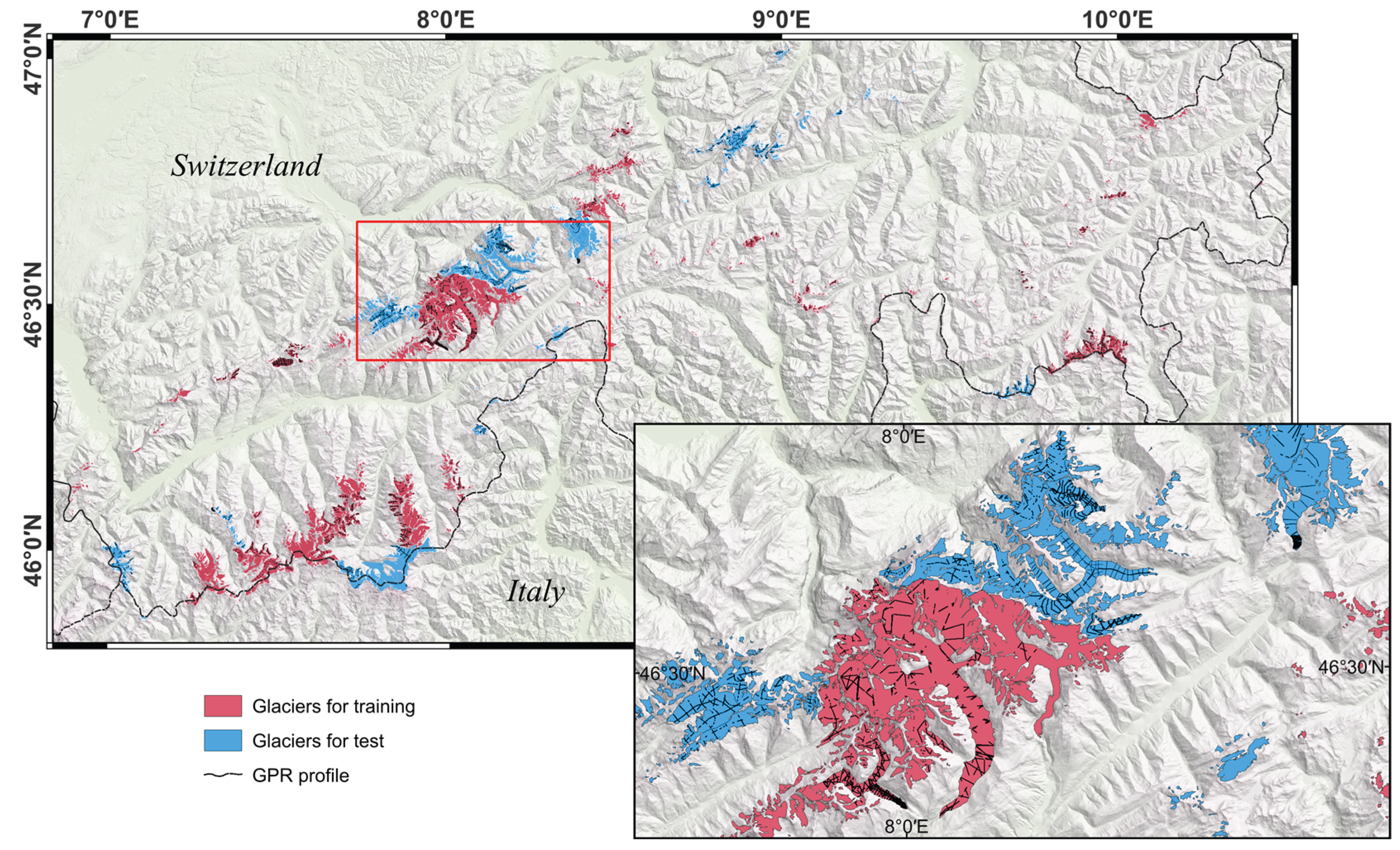
Figure 2.
Overall architecture of the CADGITE network. (a) illustrates the detailed structure of the Residual Block (Res Block), and (b) shows the detailed structure of the Residual Coordinate Attention Block (ResCA Block).
Figure 2.
Overall architecture of the CADGITE network. (a) illustrates the detailed structure of the Residual Block (Res Block), and (b) shows the detailed structure of the Residual Coordinate Attention Block (ResCA Block).
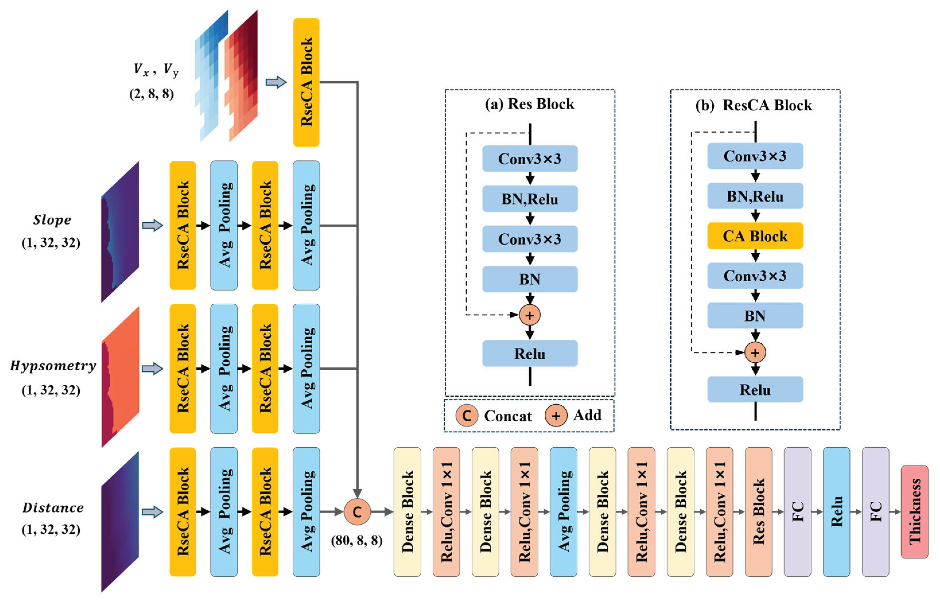
Figure 3.
Architecture of the Coordinate Attention (CA) Block.
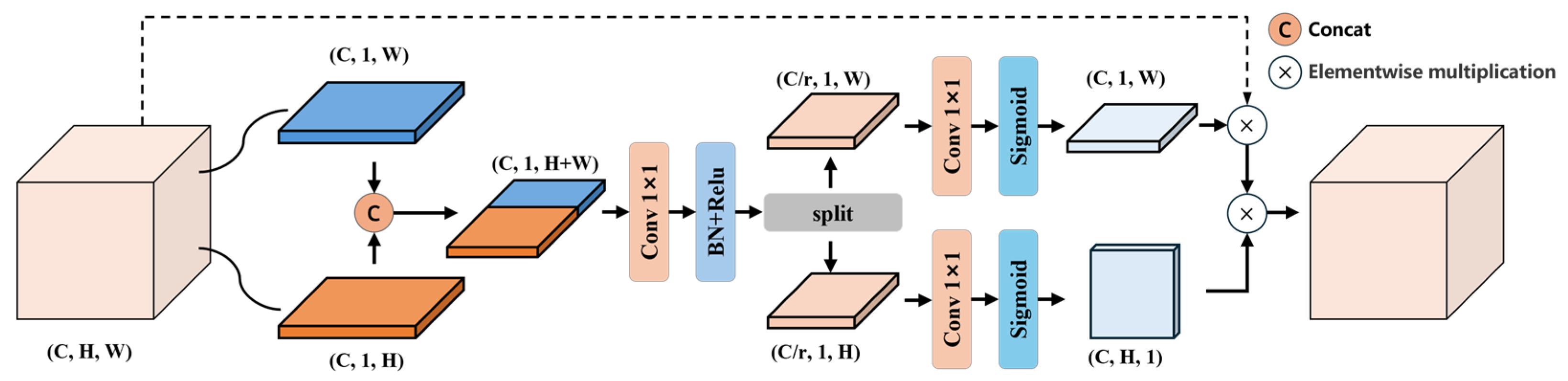
Figure 4.
Structure of the Dense Block.
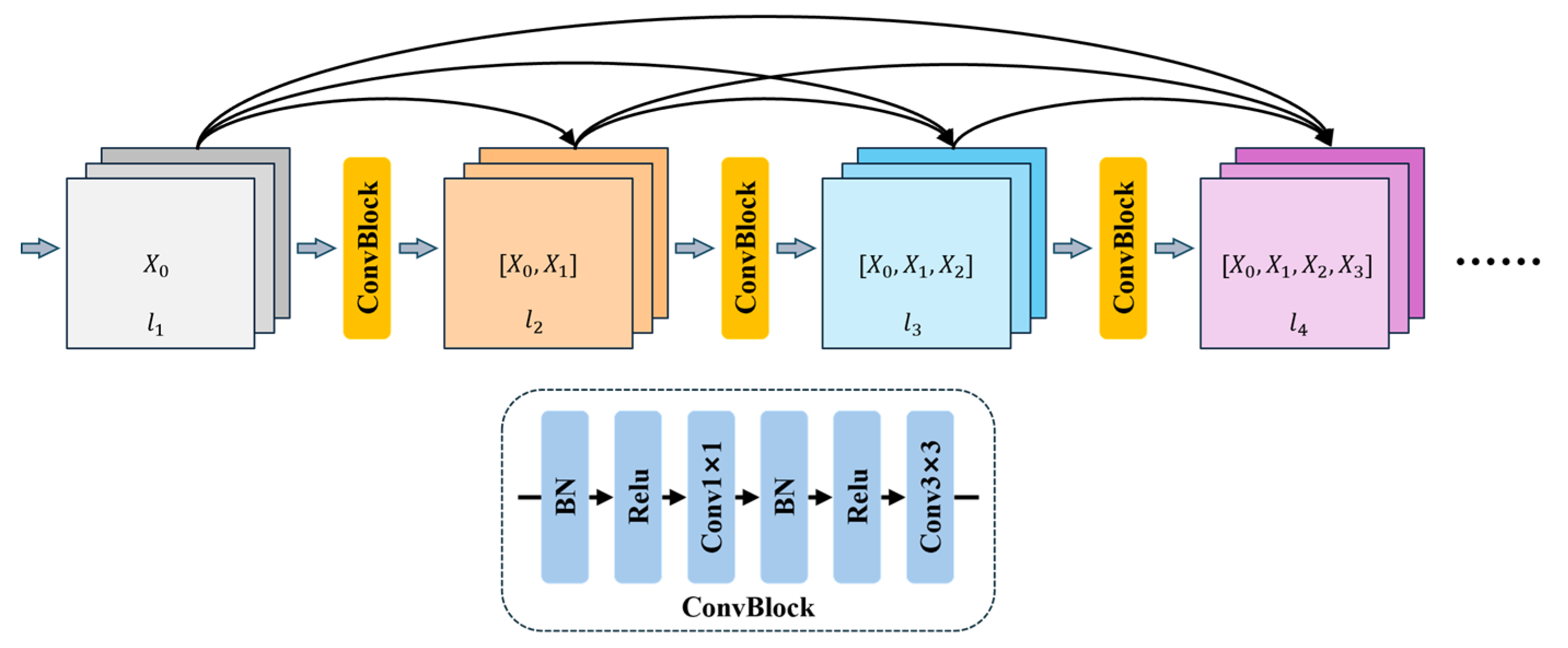
Figure 5.
Training and validation losses of the four folds. Panels (a) correspond to inputs without Distance, while panels (b) correspond to inputs with Distance.
Figure 5.
Training and validation losses of the four folds. Panels (a) correspond to inputs without Distance, while panels (b) correspond to inputs with Distance.
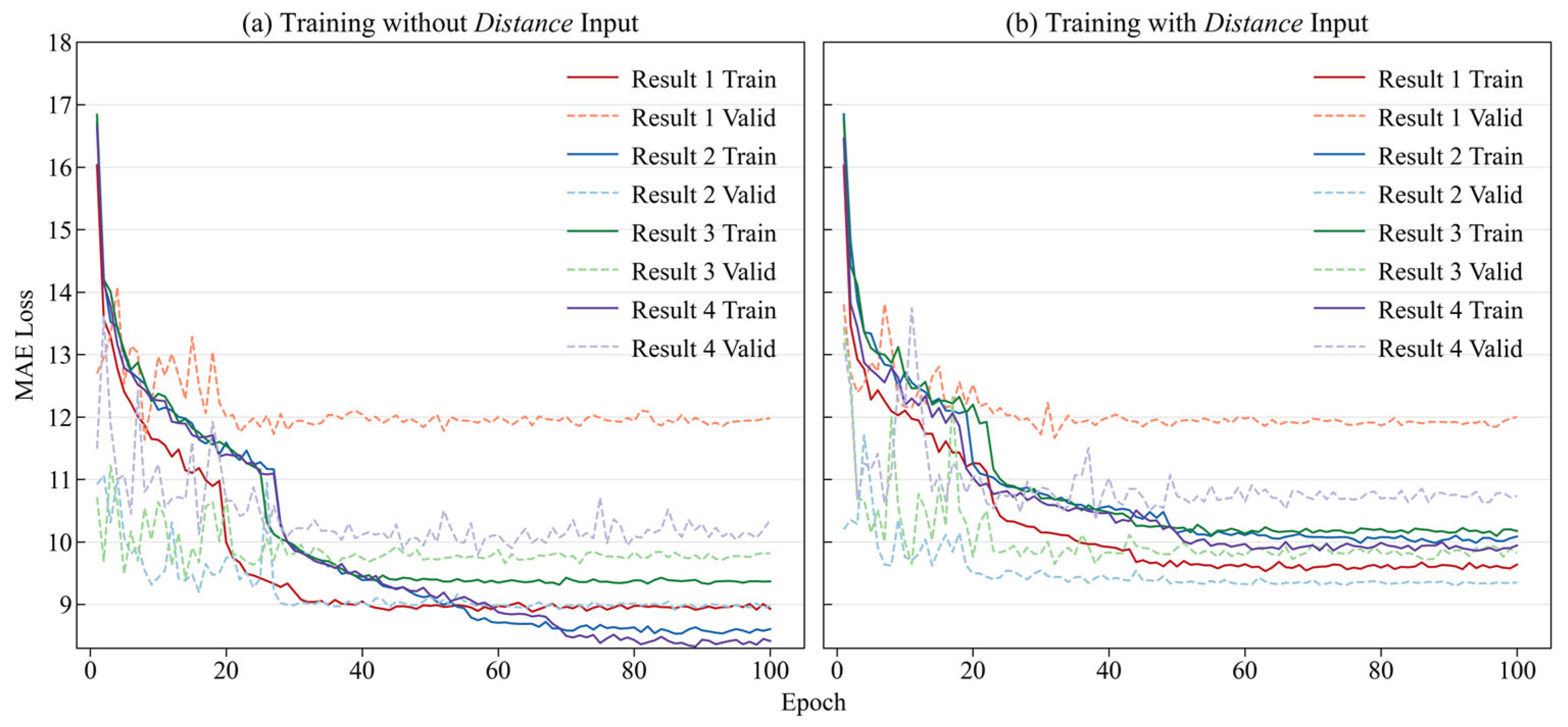
Figure 6.
Comparison between the ice thickness estimated by the models and that measured by GPR on the four folds of test glaciers. (A) CADGITE without distance to boundary input; (B) CADGITE with distance to boundary input.
Figure 6.
Comparison between the ice thickness estimated by the models and that measured by GPR on the four folds of test glaciers. (A) CADGITE without distance to boundary input; (B) CADGITE with distance to boundary input.
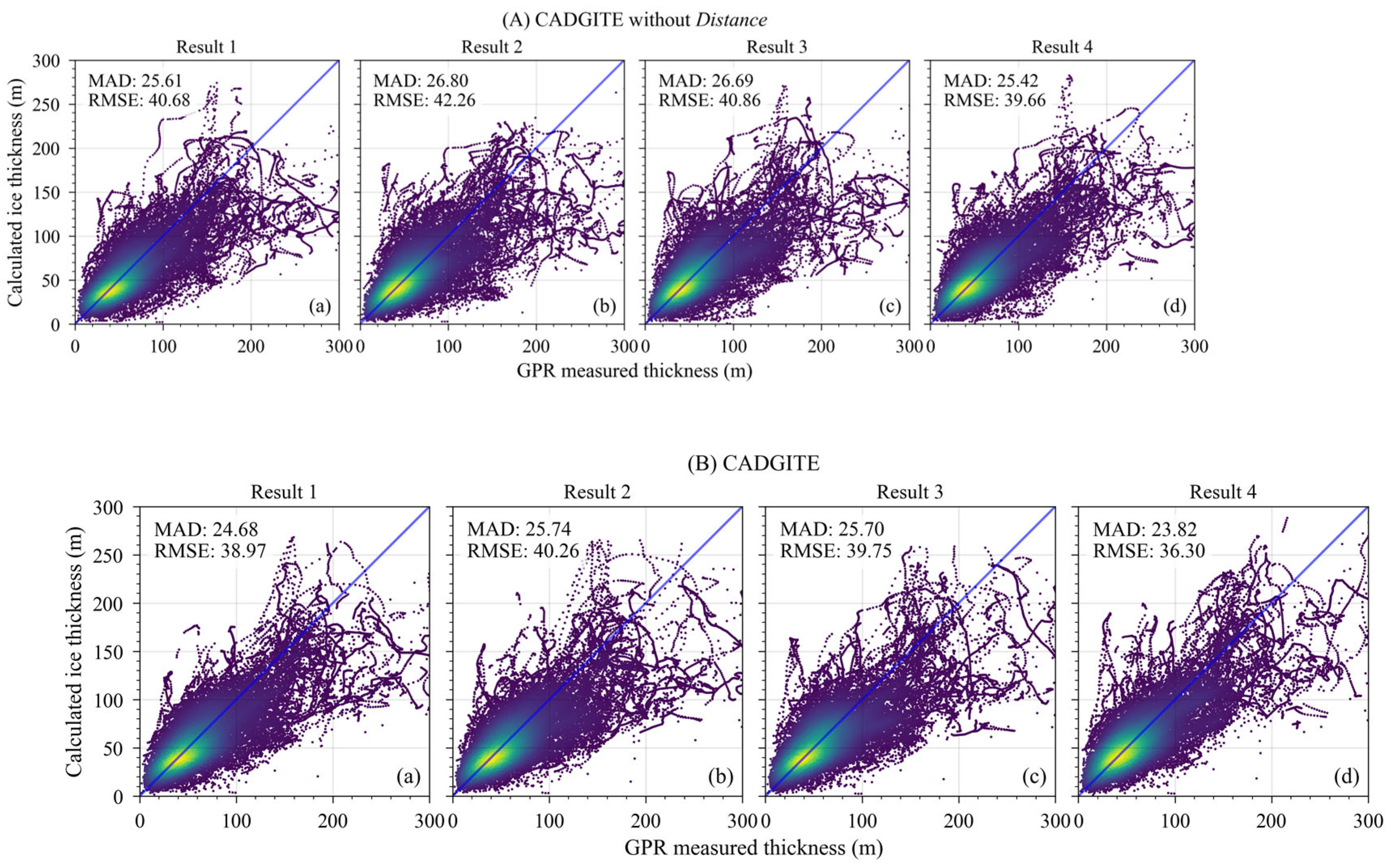
Figure 7.
Comparison between the ice thickness estimated by the LLUM model with Distance input and the GPR measurements on the four folds of the test glaciers.
Figure 7.
Comparison between the ice thickness estimated by the LLUM model with Distance input and the GPR measurements on the four folds of the test glaciers.
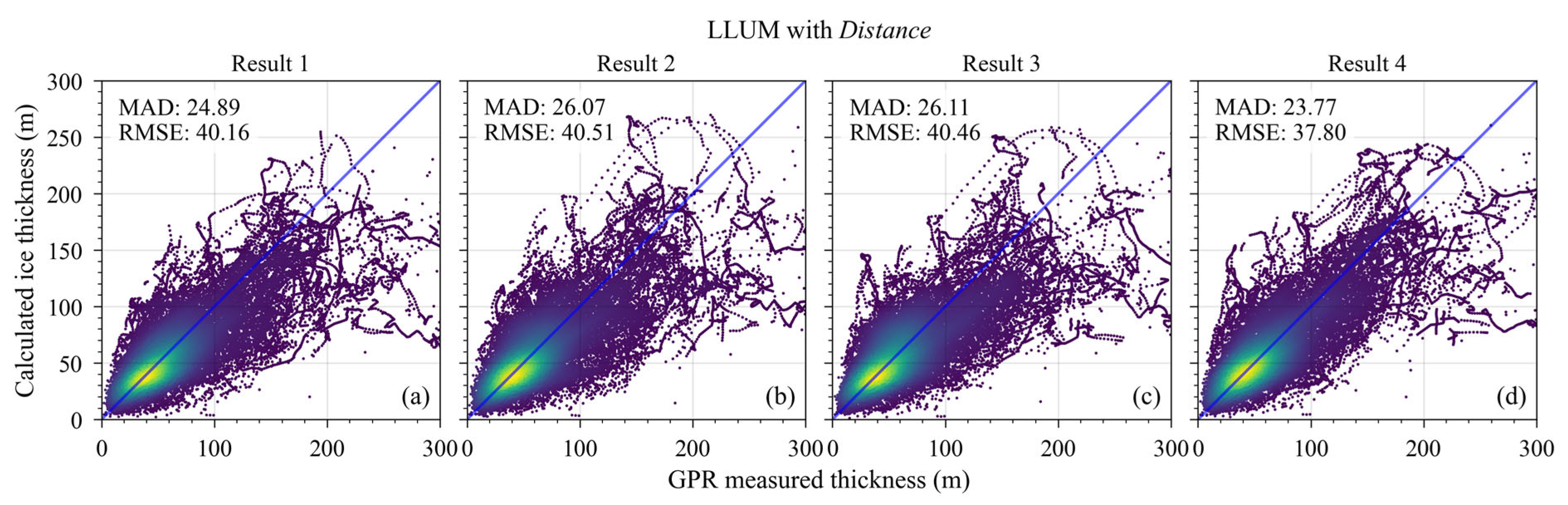
Figure 8.
Comparison between GPR measurements and ice thickness estimates from four models: Millan, H&F, GlabTop2, and CADGITE. Panel (A) shows the results on all test glacier samples, while panel (B) presents the results on test glacier samples excluding Unteraargletscher.
Figure 8.
Comparison between GPR measurements and ice thickness estimates from four models: Millan, H&F, GlabTop2, and CADGITE. Panel (A) shows the results on all test glacier samples, while panel (B) presents the results on test glacier samples excluding Unteraargletscher.
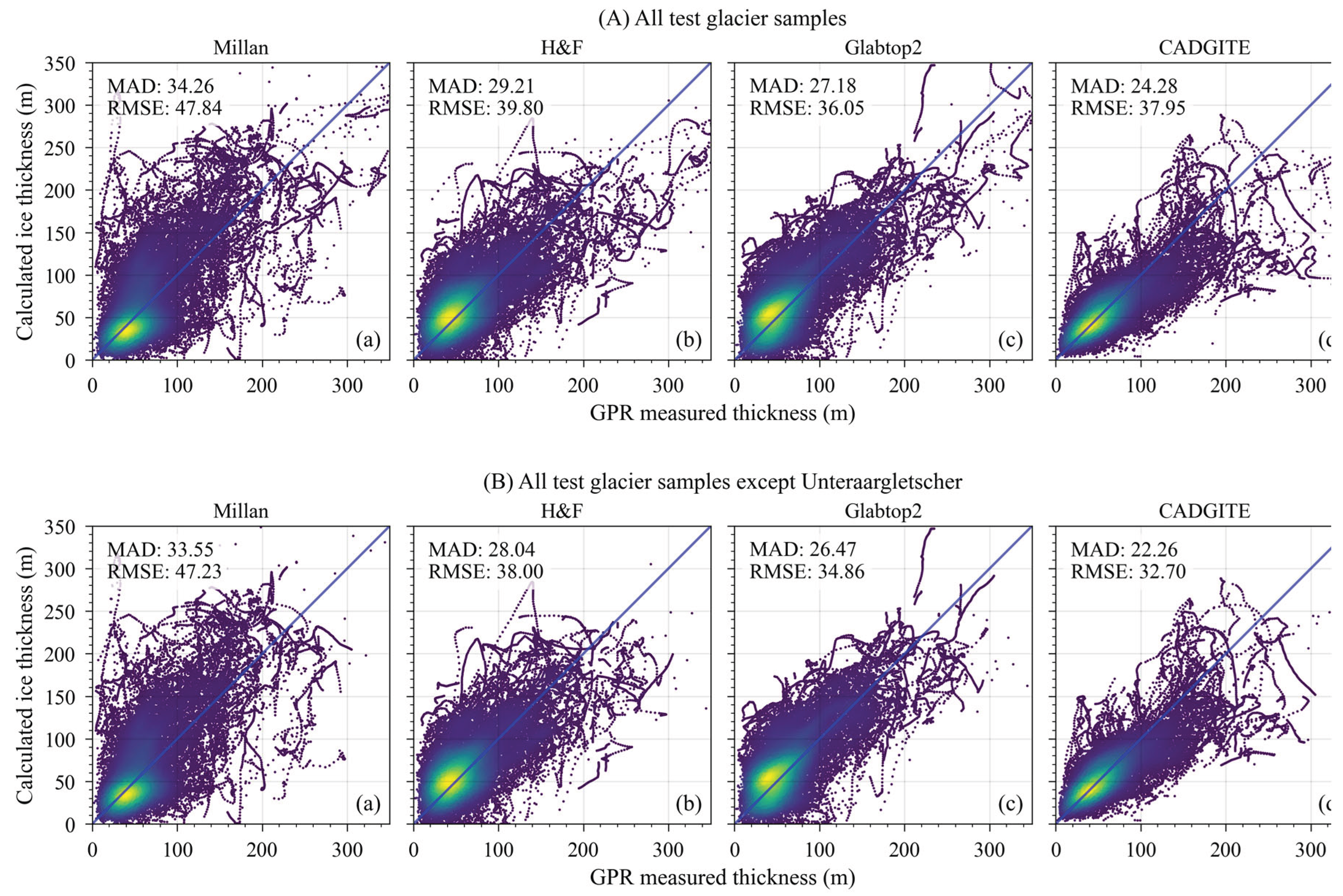
Figure 9.
Ice thickness of a part of the glaciers in Switzerland. (a) Ice thickness reference values (Grab et al., 2021), (b) and (c) show the ice thickness results modelled in this study.
Figure 9.
Ice thickness of a part of the glaciers in Switzerland. (a) Ice thickness reference values (Grab et al., 2021), (b) and (c) show the ice thickness results modelled in this study.

Figure 10.
The thickness estimation results of the CADGITE for 14 glaciers in HMA with available GPR observations.
Figure 10.
The thickness estimation results of the CADGITE for 14 glaciers in HMA with available GPR observations.
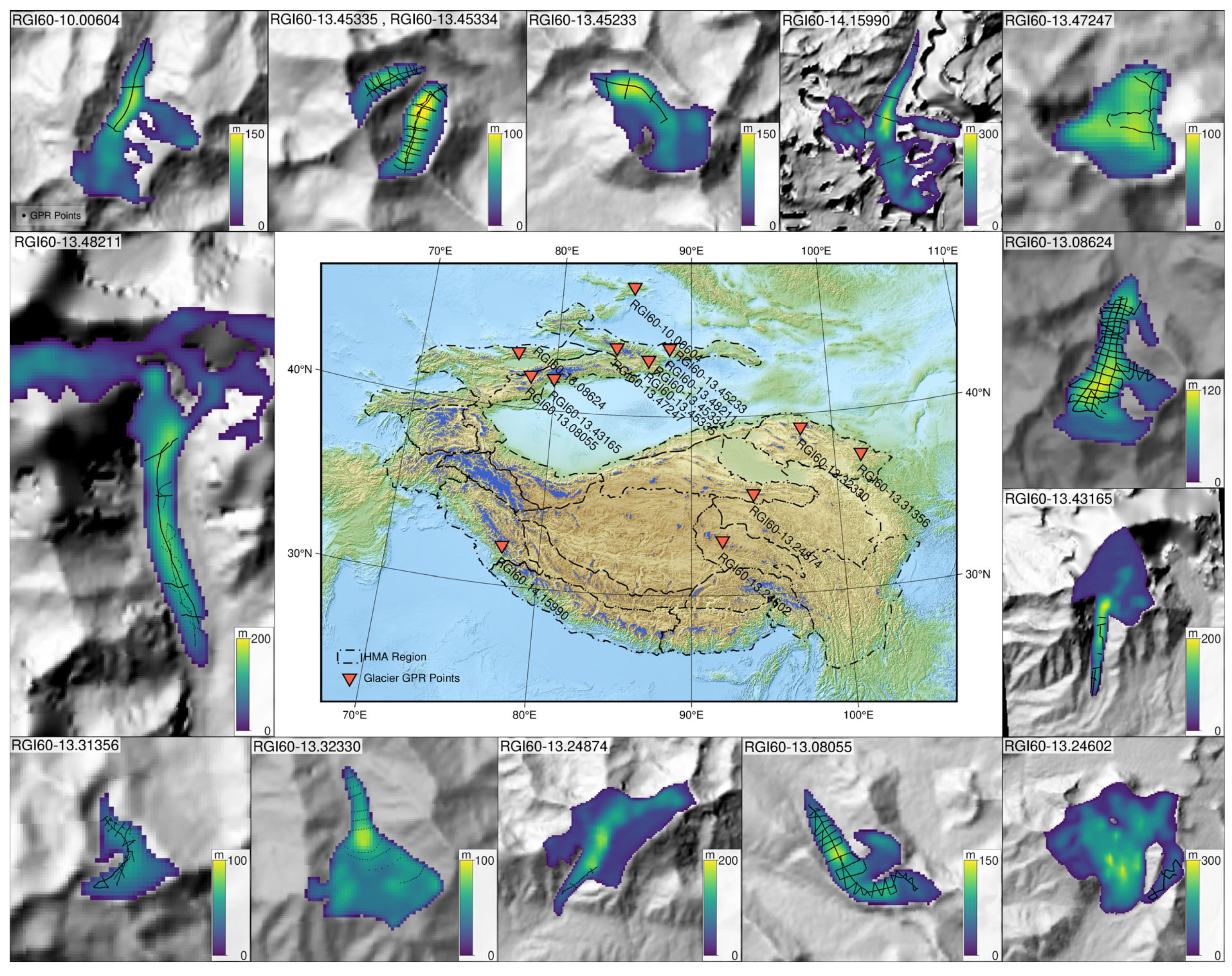
Figure 11.
Comparison of ice thickness estimates from the CADGITE model and three other models with GPR measurements across 14 Asian glaciers.
Figure 11.
Comparison of ice thickness estimates from the CADGITE model and three other models with GPR measurements across 14 Asian glaciers.
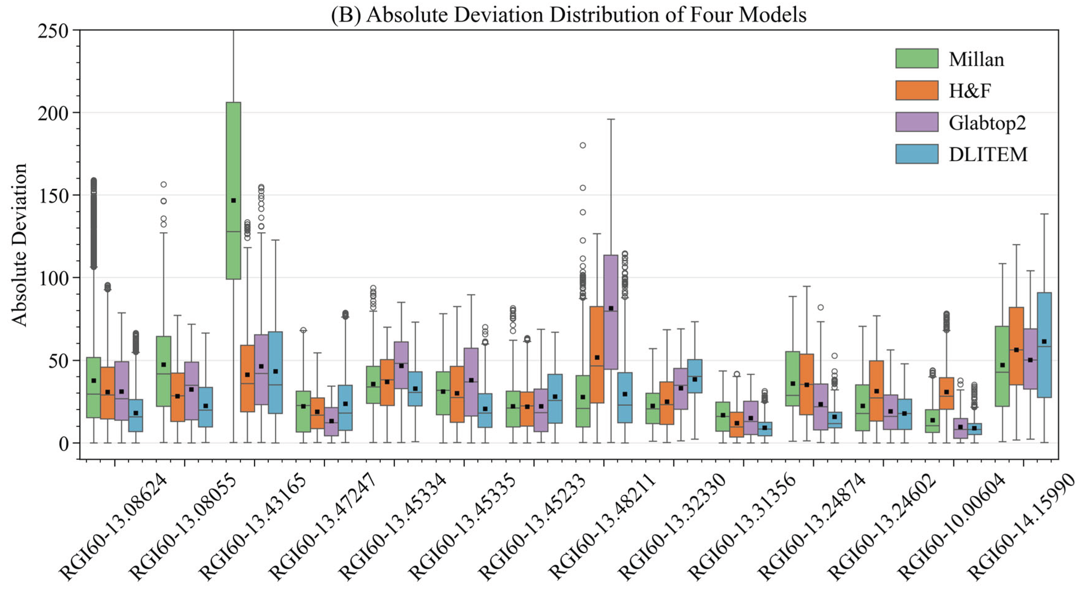
Figure 12.
A comprehensive comparison of ice thickness estimates from four models at GPR measurement points on 14 glaciers within HMA.
Figure 12.
A comprehensive comparison of ice thickness estimates from four models at GPR measurement points on 14 glaciers within HMA.
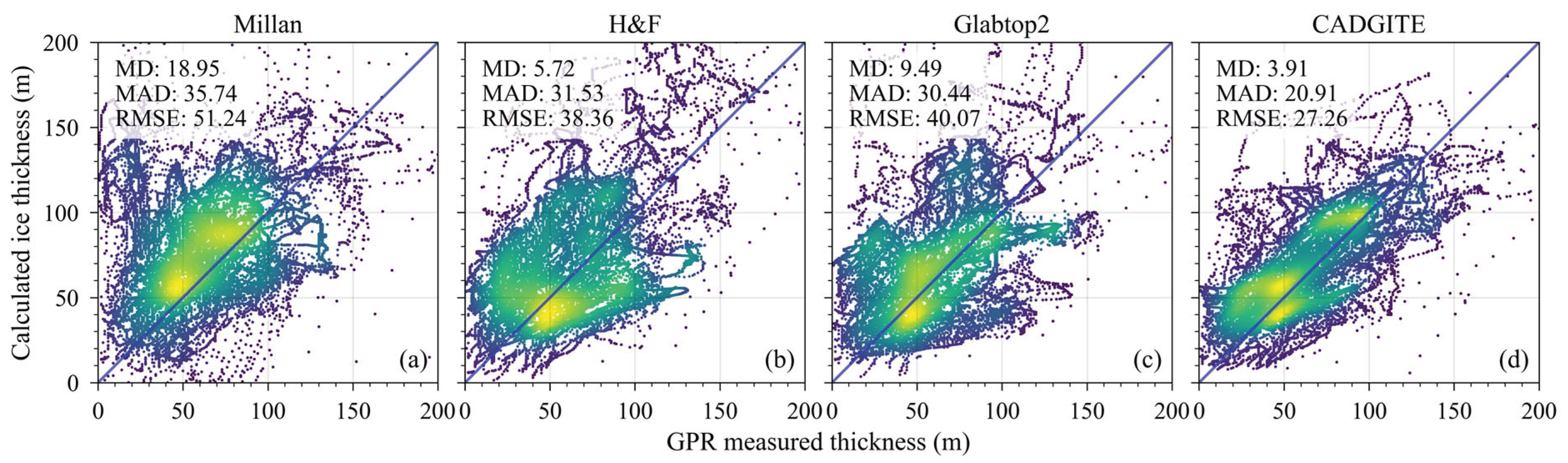
Figure 13.
The thickness distribution of the input for model training.
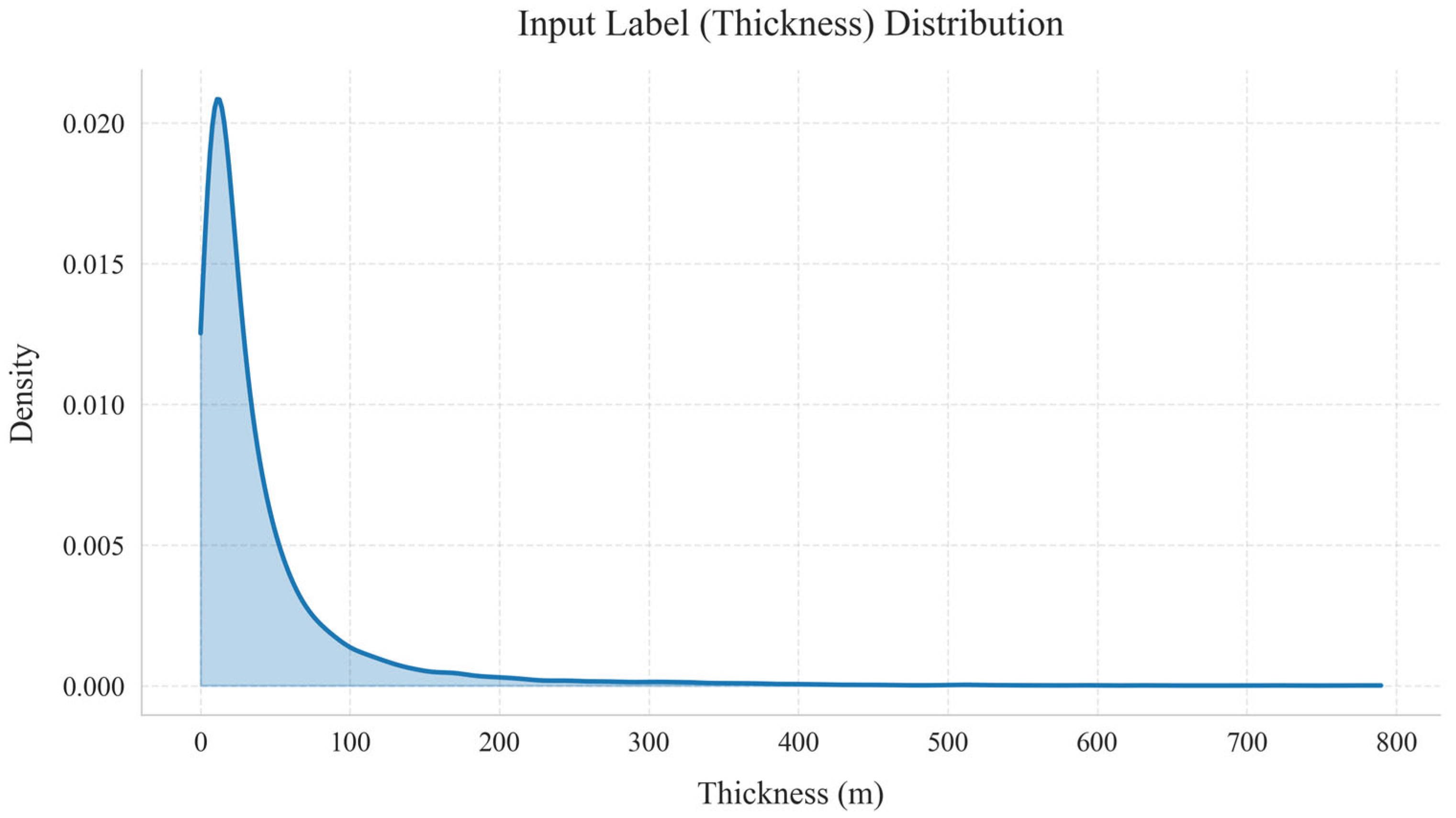
Figure 14.
(a) Slope input values for the Unteraargletscher; (b) Reference thickness values for the Unteraargletscher (Grab et al., 2021).
Figure 14.
(a) Slope input values for the Unteraargletscher; (b) Reference thickness values for the Unteraargletscher (Grab et al., 2021).
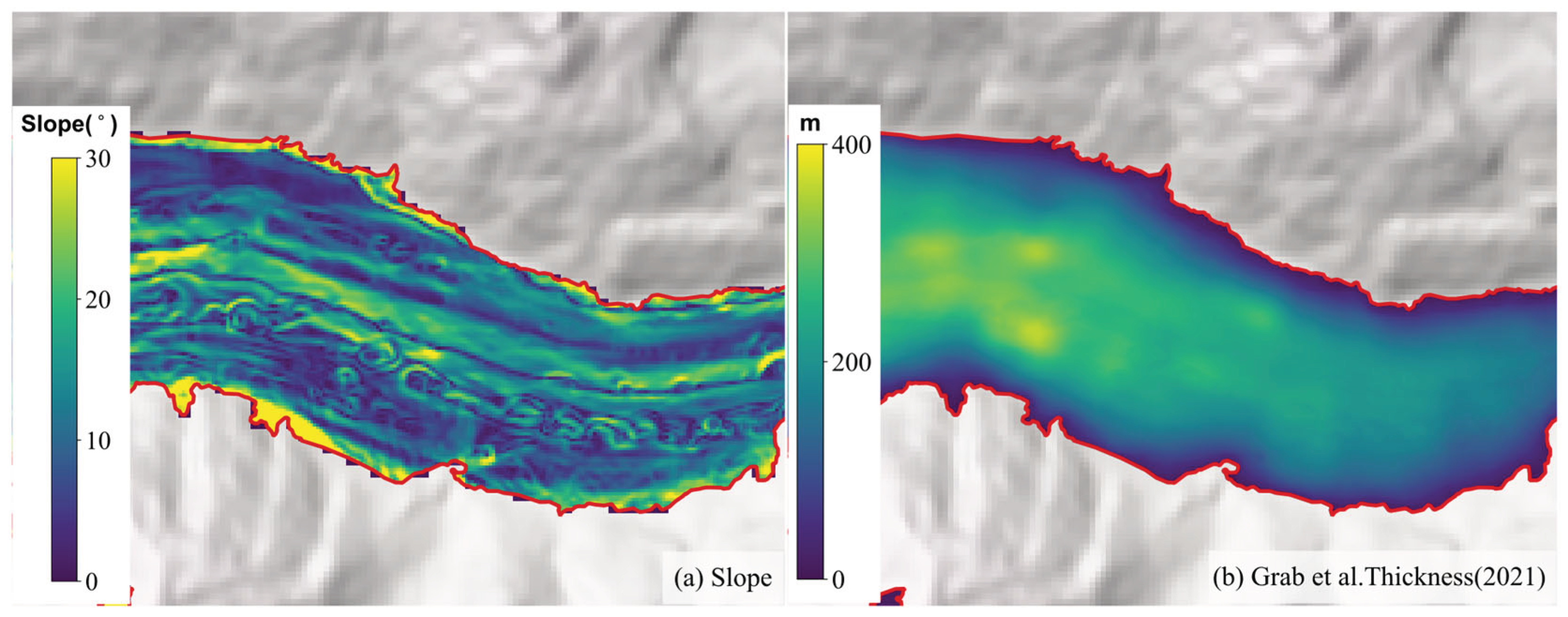

Table 1.
Loss results on the test glaciers for CADGITE from four-fold cross-validation.
| Groups | Result 1 | Result 2 | Result 3 | Result 4 |
|---|---|---|---|---|
| CADGITE without Distance | 18.40 | 18.07 | 18.01 | 17.05 |
| CADGITE | 17.28 | 18.14 | 17.44 | 16.49 |
Table 2.
Loss results on the test glaciers for LLUM from four-fold cross-validation.
| Group | Result 1 | Result 2 | Result 3 | Result 4 |
|---|---|---|---|---|
| LLUM with Distance | 17.51 | 17.89 | 17.85 | 16.37 |
Table 3.
Deviation statistics of the four models compared with GPR measurements across 14 glaciers within HMA.
Table 3.
Deviation statistics of the four models compared with GPR measurements across 14 glaciers within HMA.
| RGIId | Error Metrics | Millan | H&F | GlabTop2 | CADGITE |
| RGI60-10.00604 | MD | 4.56 | 29.37 | -0.25 | -0.27 |
| MAD | 13.62 | 30.78 | 9.62 | 8.88 | |
| RMSE | 16.89 | 34.96 | 12.45 | 10.53 | |
| RGI60-13.08055 | MD | 30.67 | 4.10 | 4.66 | -3.77 |
| MAD | 47.47 | 28.23 | 32.21 | 22.39 | |
| RMSE | 57.31 | 33.18 | 37.34 | 27.03 | |
| RGI60-13.08624 | MD | 34.30 | 23.60 | 23.91 | 10.18 |
| MAD | 37.70 | 30.81 | 31.02 | 18.05 | |
| RMSE | 48.98 | 36.50 | 37.43 | 22.58 | |
| RGI60-13.24602 | MD | -0.49 | -28.33 | -10.55 | -3.41 |
| MAD | 22.48 | 31.41 | 19.17 | 17.87 | |
| RMSE | 28.59 | 37.82 | 23.65 | 21.06 | |
| RGI60-13.24874 | MD | 29.56 | 31.70 | 22.50 | 1.67 |
| MAD | 35.82 | 35.11 | 23.45 | 15.75 | |
| RMSE | 43.03 | 41.40 | 29.61 | 19.88 | |
| RGI60-13.31356 | MD | -6.36 | 4.74 | -13.36 | -0.86 |
| MAD | 16.83 | 11.83 | 14.97 | 9.18 | |
| RMSE | 20.24 | 15.11 | 18.66 | 11.08 | |
| RGI60-13.32330 | MD | -17.03 | -22.42 | -31.87 | -38.12 |
| MAD | 22.40 | 24.89 | 32.99 | 38.51 | |
| RMSE | 26.61 | 29.65 | 36.59 | 41.93 | |
| RGI60-13.43165 | MD | 146.57 | 40.80 | 45.02 | 42.50 |
| MAD | 146.84 | 41.12 | 46.23 | 47.37 | |
| RMSE | 161.16 | 49.80 | 55.37 | 53.07 | |
| RGI60-13.45233 | MD | -9.91 | 19.45 | 18.79 | 26.00 |
| MAD | 22.00 | 21.88 | 22.11 | 27.96 | |
| RMSE | 26.62 | 25.86 | 28.39 | 33.45 | |
| RGI60-13.45334 | MD | -30.22 | -30.62 | -43.64 | -23.67 |
| MAD | 35.61 | 36.96 | 46.50 | 32.79 | |
| RMSE | 40.24 | 41.07 | 50.83 | 36.26 | |
| RGI60-13.45335 | MD | -22.54 | -26.08 | -35.58 | -5.55 |
| MAD | 31.07 | 29.92 | 38.03 | 20.53 | |
| RMSE | 35.72 | 35.52 | 44.43 | 24.98 | |
| RGI60-13.47247 | MD | 13.72 | 3.09 | 2.90 | 18.83 |
| MAD | 22.14 | 18.87 | 13.19 | 23.74 | |
| RMSE | 27.70 | 22.89 | 16.08 | 3073 | |
| RGI60-13.48211 | MD | 6.39 | 48.20 | 76.63 | -2.50 |
| MAD | 27.60 | 51.64 | 81.61 | 29.56 | |
| RMSE | 36.72 | 61.76 | 95.67 | 37.75 | |
| RGI60-14.15990 | MD | -17.82 | -16.48 | -8.82 | -49.90 |
| MAD | 47.07 | 56.23 | 50.19 | 61.28 | |
| RMSE | 55.16 | 63.00 | 55.42 | 73.31 |
Disclaimer/Publisher’s Note: The statements, opinions and data contained in all publications are solely those of the individual author(s) and contributor(s) and not of MDPI and/or the editor(s). MDPI and/or the editor(s) disclaim responsibility for any injury to people or property resulting from any ideas, methods, instructions or products referred to in the content. |
© 2025 by the authors. Licensee MDPI, Basel, Switzerland. This article is an open access article distributed under the terms and conditions of the Creative Commons Attribution (CC BY) license (http://creativecommons.org/licenses/by/4.0/).
Copyright: This open access article is published under a Creative Commons CC BY 4.0 license, which permit the free download, distribution, and reuse, provided that the author and preprint are cited in any reuse.


