
Submitted:
29 May 2025
Posted:
29 May 2025
You are already at the latest version
Abstract
This study evaluates machine learning-based methods for retrieving thin Arctic sea ice thickness (SIT) from L-band radiometry, using data from ESA’s Soil Moisture and Ocean Salinity (SMOS) satellite. Alongside the operational ESA product, three alternative approaches are assessed: a Random Forest (RF) algorithm, a Convolutional Neural Network (CNN) that incorporates spatial coherence, and a Long Short-Term Memory (LSTM) neural network designed to capture temporal coherence. Validation with in situ data from the BGEP moorings and the IRO2/ESA SMOSice campaign shows that the RF algorithm achieves robust performance comparable to the ESA product, despite its simplicity and lack of explicit spatial or temporal modeling. The CNN exhibits a tendency to overestimate SIT and shows higher dispersion, suggesting limited added value when spatial coherence is already present in the input data. The LSTM approach does not improve retrieval accuracy, likely due to the mismatch between satellite resolution and the temporal variability of sea ice conditions. These results highlight the importance of L-band sea ice emission modeling over increasing model complexity and suggest that simpler, adaptable methods such as RF offer a promising basis for future SIT retrieval efforts. The findings are relevant for refining current methods used with SMOS and for the development of upcoming satellite missions, such as ESA’s Copernicus Imaging Microwave Radiometer (CIMR).
Keywords:
machine learning
; remote sensing
; sea ice
; cryosphere
1. Introduction
Sea ice is a key component of the Earth system. Its extent undergoes an annual periodicity and covers almost 7% of the Earth’s surface at its maximum extent in September, mainly the poles. It has a crucial effect on climate change, as it participates in the so-called ice-albedo feedback loop [1]. Arctic sea ice has been significantly decreasing in recent decades [2], also suffering a shift to younger and thinner ice [3].
Since the launch of the first Earth Observation (EO) satellites in the early 1970s, passive microwave radiometers have been used to observe sea ice. The European Space Agency (ESA) mission Soil Moisture and Ocean Salinity (SMOS) [4,5], initiated in 2009, and NASA’s Advanced Microwave Scanning Radiometer (AMSR) series, which operated on different satellites from 2002 to the present, as well as the Soil Moisture Active Passive (SMAP) [6] mission, launched on 2015, are key contributors. In particular, the focus of this study is passive L-band radiometers such as SMOS, working at 1.4 GHz with a penetration depth of up to 1 m or even more in low salinity sea ice.
Currently, two distinct algorithms for estimating Arctic thin sea ice thickness from SMOS measurements during the non-melting period (October to April) exist. The first, distributed by the European Space Agency (ESA), is a semi-empirical algorithm developed by the Alfred Wegener Institute (AWI) as described in [7] and [8]. However, a significant drawback is its inability to consider the presence of snow atop sea ice. This limitation is critical due to the substantial impact of snow on emitted L-band radiation [9] and subsequent thickness retrieval processes. The second algorithm, from the University of Bremen (UB) and detailed in [10], adopts an empirical approach. Despite this, a notable limitation of the UB product is its restricted sensitivity, reaching only up to 0.5 m. While the UB product explicitly limits the sea ice thickness retrieval, the AWI product does not have a clearly defined upper limit, with sensitivity typically ranging between 0.5 and 1.5 m depending on sea ice conditions.
Other emerging methodologies include the use of Global Navigation Satellite System Reflectometry (GNSS-R), which, beyond its previous applications to retrieve various geophysical parameters, has also been explored for sea ice applications. Recent studies have shown its potential to detect sea ice and estimate its thickness, although these results have so far only been demonstrated in simulations [11,12]. Nevertheless, GNSS-R remains promising as a valuable complement to passive L-band measurements in the future.
Artificial Intelligence (AI) holds the potential to transform the processing and analysis of Earth Observation (EO) data acquired through remote sensing. AI offers the capability to improve the analysis of these data, enhancing our ability to monitor and predict the evolution of many geophysical variables. Recent efforts to retrieve sea ice parameters from satellite observations using artificial intelligence have increasingly focused on applying machine learning techniques to passive microwave data. One of the earlier examples is found in [13], where a neural network was used to try to estimate snow depth over sea ice using AMSR2 and SMOS data. Similarly, [14] applied two machine learning algorithms to retrieve sea ice thickness from a combination of TechDemoSat-1 (TDS-1) and SMOS observations. [15] developed an ensemble convolutional neural network (CNN) to retrieve daily sea ice thickness from AMSR2 data. Likewise, [16] and [17] used a combination of frequencies ranging from 1.4 to 36 GHz, applying AI-based methodologies to estimate and analyze sea ice thickness and volume trends. Beyond SMOS and AMSR2, [18], used a neural network to retrieve sea ice thickness from FSSCat nanosatellite data [19]. Meanwhile, [20] and [21] investigated machine learning approaches for sea ice sensing using data from a C-band Synthetic Aperture Radar (SAR) sensor like Sentinel-1.
An application of machine learning to Arctic sea ice thickness retrieval from SMOS observations was presented in [22]. That study employed two decision-tree-based algorithms—Random Forest (RF) and Gradient Boosting (GB)—within a supervised learning framework. These algorithms were trained on data derived from maps generated through model inversion. The results were promising, demonstrating good agreement with ESA’s sea ice thickness product and achieving improved validation against in situ datasets. Building on this foundation, the objective of this work is to assess the performance of deep learning methods in enhancing the retrieval accuracy. Specifically, it extends the methodology by implementing a Convolutional Neural Network (CNN) and a Long Short-Term Memory (LSTM) neural network. These approaches represent significant advancements in data processing: the CNN leverages spatial coherence by treating input variables as maps, while the LSTM captures temporal coherence by utilizing sequential information from consecutive observations.
Section 2 describes the various data sources used as input, the generation of the training dataset, and the datasets employed for validation. Section 3 outlines the different algorithm approaches. The results of the assessment are presented in Section 4, followed by a discussion in Section 5. Finally, the conclusions of the study are summarized in Section 6.
2. Data Collection and Processing
This section describes the datasets used both as input variables for the proposed algorithms and as in situ observations for their validation. Additionally, it provides details on data preparation and the processing steps performed to generate the training dataset.
2.1. Input Datasets
The input variables are composed by a combination of satellite-derived products and reanalysis model outputs, providing a comprehensive coverage of Arctic sea ice conditions. The satellite datasets include the ESA’s SMOS sea ice thickness product, from which only the TB is extracted and used as input, and a sea ice surface temperature data product. Additionally, a reanalysis model provides required information about sea ice and seawater properties. The final subsection explains how these variables are processed to be used as input for the proposed methodology.
2.1.1. ESA SMOS Sea Ice Thickness Product
The SMOS satellite carries the Microwave Imaging Radiometer Aperture Synthesis (MIRAS) payload, which measures the brightness temperatures in full polarization at L-band with incidence angles ranging from 0° to 65°, including all four Stokes parameters [23]. The instrument provides global coverage every three days and daily coverage in the polar regions. The hexagonal two-dimensional snapshots taken by the MIRAS instrument have a spatial dimension of around 1200 km across and can capture brightness temperature every 1.2 seconds, and the spatial resolution varies from about 35 km at nadir view to over 50 km at higher incidence angles. Each snapshot measures one of the Stokes components in the antenna reference frame, including horizontally (TBH) and vertically (TBV) polarized brightness temperatures. The intensity is obtained by averaging the horizontally and vertically polarized brightness temperatures. Moreover, the brightness temperature (TB) intensity of the signal over sea ice remains relatively consistent regardless of the angle at which it is measured within the range, and thus it is computed as an average of this interval. The daily averaged brightness temperature intensity in the Arctic region is interpolated using a nearest neighbor algorithm and gridded into the National Snow and Ice Data Center (NSIDC) polar stereographic projection with a grid resolution of 12.5 km.
The SMOS L3 Sea Ice Thickness product is produced by AWI and distributed by the ESA, and it provides information on sea ice thickness in the Arctic region from October to April, covering the period from 2010 to the present. It was first described in [7] and [8]. The sea ice thickness is determined using an iterative retrieval algorithm that incorporates a thermodynamic sea ice model and a three-layer radiative transfer model. The radiative transfer model calculates the emissivity of the sea ice layer and the underlying seawater, and brightness temperatures are derived from the emissivity and physical temperatures of the sea ice and seawater. The bulk ice temperature is estimated using a thermodynamic model, which utilizes the 2 m air temperature from atmospheric reanalysis data as an input parameter, while the bulk ice salinity is computed from an empirical relation described in [24]. The retrieval algorithm also accounts for variations in ice thickness within the SMOS spatial resolution by using a statistical thickness distribution function based on high-resolution ice thickness measurements from NASA’s Operation IceBridge (OIB) campaign.
In this work, the brightness temperature (TB) intensity maps measured by SMOS are taken from the ESA/AWI SMOS sea ice thickness product (https://earth.esa.int/eogateway/catalog/smos-l3-sea-ice-thickness) and used as input for the algorithms. Consequently, all processing details related to the TB, including the handling of the angular distribution of satellite measurements, are described in the product’s Algorithm Theoretical Basis Document (ATBD, [25]).
2.1.2. Surface Temperature Satellite Product
The Arctic Ocean - Sea and Ice Surface Temperature Reprocessed product [26], produced by Danish Meteorological Institute (DMI) and distributed by Copernicus Marine Service (CMEMS), provides information on Arctic sea and ice surface temperatures. This data is derived from reprocessed observations obtained through the Advanced Very High Resolution Radiometer (AVHRR), the Advanced Along Track Scanning Radiometers (AATSR), and the Sea and Land Surface Temperature Radiometer (SLSTR). These observations come from different sources, including the ESA Climate Change Initiative (CCI) project, the Copernicus Climate Change Service (C3S) project, and the Arctic & Antarctic Ice Surface Temperatures from Thermal Infrared Satellite Sensors (AASTI) dataset. The product presents a daily interpolated field at a resolution of 0.05 degrees, encompassing surface temperatures in the ocean, sea ice, and the marginal ice zone. The computation of surface temperature employs the optimal interpolation method, with the previous day’s value serving as the initial guess field.
In this work, a linear temperature gradient within the ice is assumed, as supported by findings in [27]. Consequently, the calculation of the bulk ice temperature () is determined by the following expression:
where is the surface temperature obtained from the satellite product, and is the seawater temperature, in which a typical value for the Arctic of is assumed.
2.1.3. Arctic Ocean Physics Reanalysis Model
The Arctic Ocean Physics Reanalysis model, produced by Nansen Environmental and Remote Sensing Center (NERSC) and distributed by CMEMS [28], presents physical variables derived from the reanalysis model TOPAZ (version 4b). This model assimilates a diverse set of observations, including sea level anomalies from satellite altimeters, sea surface temperature from Operational Sea Surface Temperature and Sea Ice Analysis (OSTIA), in situ temperature and salinity data from hydrographic cruises and moorings, sea ice concentration from OSI-SAF, CS2SMOS ice thickness data, and sea surface salinity from the Barcelona Expert Center (BEC) utilizing SMOS satellite data.
In this work, the seawater salinity, the sea ice thickness and the snow depth variables are collected from this model. To compute the sea ice salinity, an empirical formula from [24] is used:
where is the seawater salinity and the sea ice thickness in cm, both obtained from the Arctic Ocean Physics Reanalysis model. The growth rate coefficient, denoted as a, ranges between 0.35 and 0.5; , the salinity ratio of the bulk ice salinity at the end of the ice growth season, is also crucial to determine the empirical equation for the sea ice salinity. [24] proposes using a value of 0.5 for a and 0.13 for . However, [29] suggests using 0.175 for instead of 0.13 after comparing equation 2 with observed data in the Arctic.
Ultimately, the determination of the snow presence variable is based on a straightforward assumption: If the snow thickness variable derived from TOPAZ is positive, it is inferred that snow is present; conversely, if it is zero, snow is considered absent.
2.2. Training Dataset Generation Through Model-Based Simulation
The data available for the Arctic region is extremely limited. Due to the absence of a comprehensive dataset on thin sea ice thickness, it becomes necessary to create one through the use of sea ice emission modeling. The Burke emission model [30], incorporating the Vant formulation for ice permittivity [31], is employed in an inverted manner to generate realistic scenarios of Arctic sea ice thickness distributions. The goal is to replicate situations as accurately as possible. All the variables, i.e. the SMOS TB, the sea ice temperature and salinity, and the snow presence, are previously regridded to the 12.5 km x 12.5 km NSIDC Polar Stereographic grid. This workflow to generate the training dataset is summarized in Figure 1. Noteworthy, the sensitivity of brightness temperature to ice thickness in this frequency band is strongly influenced by ice conditions, specifically temperature and salinity. To avoid the imposition of an artificial training threshold, the maximum thickness that can be retrieved (the point at which brightness temperature saturation begins) is computed for each configuration of ice conditions. Subsequently, the thickness derived from the model inversion is compared to this maximum thickness. If the latter is smaller, the inverted solution is adjusted to match this maximum thickness.
The accuracy of this model-based simulation fundamentally depends on the performance of the L-band sea ice emission modeling. However, it is currently not possible to quantify its precision due to the lack of Arctic-wide ground truth observations. The Burke model, originally developed for soil applications, has been widely adopted as an incoherent approach for simulating sea ice emission. Alternatively, a coherent approach could be considered [32], since coherence effects may arise when two or more interfaces exist within a plane-parallel medium, allowing an electromagnetic plane wave to interfere with its reflected counterpart [10]. Nevertheless, these effects are generally assumed to be averaged out over the satellite footprint, and to date, no significant influence has been confirmed. More complex radiative transfer models, such as the Snow Microwave Radiative Transfer model (SMRT, [33]), which account for internal scattering within the medium, are not necessary in this context, as such effects are negligible at L-band frequencies. The main source of uncertainty in modeling sea ice emission lies in the dielectric constant. As discussed in [27] and [34], the Vant formulation is comparable to theoretical models that treat sea ice as a mixture of pure ice and brine. The brine component, with its variable shapes and properties, plays a critical role in the emission process. However, there is still no consensus on which permittivity formulation is the most accurate, as it depends on the growth conditions of the sea ice, information that is not known during satellite-based sea ice thickness retrieval. Nonetheless, the combination of the Burke model with the Vant permittivity formulation appears to be a robust choice [34], capable of realistically reproducing the L-band emission of snow-covered sea ice across the Arctic.
2.3. Validation Datasets
The in situ data used in the validation is based on measurements from moored sensors in two locations of the Arctic Ocean, along with data from a campaign conducted in the Barents Sea in 2014, which unexpectedly -for the time of the year- encountered thin sea ice.
2.3.1. BGEP Mooring Data
The Upward-Looking Sonar (ULS) mooring buoys within the Beaufort Gyre Exploration Project (BGEP) are specifically designed for measuring the sea ice draft, representing the portion of sea ice submerged underwater. Consequently, to derive the total thickness of sea ice, a conversion is necessary. Following the approach outlined in [35], an empirical factor of 1.136 is applied to multiply the ice draft, thus providing the total thickness. This coefficient was determined through an empirical analysis that included nearly 400 sea ice drillings conducted in the Fram Strait [36]. The BGEP ULS data, consisting of daily averages of sea ice thickness from three mooring instruments situated within the Beaufort Gyre, serves as a one of the datasets for validating the methodology.
2.3.2. Barents 2014: IRO2/ESA SMOSice Campaign
The IRO2/ESA SMOSice campaign took place in March 2014 in the Barents Sea ice marginal zone, concretely on newly formed thin sea ice in the south-east of Svalbard. It includes measurements collected by a helicopter operating from RV Lance and the research aircraft Polar 5 [37]. Sea ice thickness was determined utilizing an electromagnetic induction system positioned at the bow of RV Lance (SEM), as well as another EM system towed beneath the helicopter (HEM). Furthermore, a Riegl VQ-580 laser scanner (ALS) mounted on the Polar 5 aircraft was used to measure the sea ice freeboard, which was later converted to sea ice thickness by assuming hydrostatic equilibrium. All these data has been regridded to the ESA SMOS sea ice thickness product 12.5 km grid by the arithmetic average calculated with GMT blockmean [38], courtesy of Dr. Lars Kaleschke.
3. Methodology
This study introduces approaches to sea ice thickness estimation that incorporate both spatial and temporal coherence into the modeling process. Spatial coherence is achieved by utilizing maps as input data, allowing the influence of neighboring pixels to be considered, while temporal coherence is addressed by including data from the previous day to enhance predictions of current conditions. The primary objective is to evaluate and determine the most effective approach among the proposed methods, leaving uncertainty computation as a focus for future work. In previous research [22], Random Forest (RF) and Gradient Boosting (GB) algorithms were trained using a pixel-by-pixel methodology. Although these models demonstrated strong agreement with ESA’s sea ice thickness product and showed improved correlation with reduced error when validated against in situ datasets, this approach inherently breaks the spatial and temporal continuity present in the original data. In reality, the data exhibit clear spatial and temporal dependencies, and failing to account for them may limit the physical consistency of the predictions. Therefore, this study addresses a necessary step: evaluating whether preserving spatial coherence (as with CNN) or temporal continuity (as with the LSTM) leads to more physically meaningful and accurate sea ice thickness retrievals. For the three proposed approaches, the input variables are prepared as detailed in Section 2.2, with some concrete modifications for each of them that are later described. It is important to mention that despite Sea Ice Concentration (SIC) is indeed a major source of uncertainty in sea ice thickness retrievals from L-band radiometry, it is not explicitly included in this assessment, as the comparison is restricted to locations where the ESA product provides valid thickness values. This product assumes 100% SIC, justified by the fact that most ice-covered areas in winter have SIC >90%, and that uncertainties in SIC products could introduce larger errors than the underestimation caused by assuming full ice cover [7,8]. Therefore, to ensure a fair comparison, no SIC correction is applied in this study.
Three different machine learning algorithms are evaluated, but they all rely on the same presented methodology and use the same input and output variables, which are described in Section 2.1 and summarized in Figure 1. Specifically, the four input variables are: SMOS brightness temperature, sea ice temperature, sea ice salinity, and snow presence. The output variable is sea ice thickness, which, during the training phase, corresponds to the values derived from the inversion of the emission model, as detailed in Section 2.2.
3.1. Pixel-by-Pixel Approach: Random Forest & Gradient Boosting
Concentrating on supervised learning, specifically within the realm of regression methods, the machine learning algorithms chosen for this task include Random Forest (RF, [39]) and Gradient Boosting (GB, [40]). These algorithms serve as more robust extensions of decision trees, sharing numerous similarities but diverging in their approaches to tree construction and combination. Both algorithms are configured with 50 estimators, a reasonable choice after experimenting with other options ranging from 10 to 1000. Following thorough testing, no further hyperparameters are fine-tuned as there is no discernible improvement in results. Individual data points are extracted from comprehensive Arctic sea ice thickness distribution maps and fed into these algorithms for training. Therefore, this approach is named pixel-by-pixel, as the training is done only accounting for individual values within the distribution. The training dataset is composed of the 100.000 pixels extracted from the maps of each day, after dropping the duplicates, from 15th October 2019 to 15th April 2020 and from 15th October 2020 to 15th April 2021. Both RF and GB algorithms provide similar results, but in this work the RF is selected to be assessed with the other approaches.
3.2. Spatially-Coherent Approach: Convolutional Neural Network
Convolutional Neural Networks (CNN; [41]) are a class of deep learning neural networks primarily designed to process and analyze visual data. In this work, the aim is to take advantage of its potential to deal with images and introduce spatial coherence in the algorithm. Sea ice pixels are not independent of their neighbors: similar conditions should lead to similar thickness distributions. All variables in the selected grid are arrays of shape 896 x 608. The convolutional layers have a 3 x 3 kernel with padding to do not reduce the dimension of the variables within the network architecture.
After tuning the hyper-parameters, the batch size is fixed to 64 with 200 training epochs. The best combination of the number of layers and filters for each convolution is presented in Table 1. Each convolutional layer has 6, 12 or 24 filters of size 3x3 to the input image. The ReLu activation function is used to introduce non-linearity, and combined with padding configured as same ensures that the spatial dimensions of the output feature maps remain the same as the input. Batch normalization is applied after each convolutional layer. It normalizes the activation of the previous layer, helping to stabilize and speed up the training process. The last convolutional layer has 1 filter of size 3x3. The linear activation function means that there is no activation function applied to the output, which makes this layer essentially performing a linear transformation.
The training dataset is conformed by 181 maps extracted from the period that expands from 15th October 2019 to 15th April 2020 and from 15th October 2020 to 15th April 2021.
3.3. Temporally-Coherent Approach: Long Short-Term Memory Neural Networks
Despite the robust performance that can be achieved with the CNN by including its inherent spatial-coherence, the temporal coherence shall be explored. Therefore, the Long Short-Term Memory (LSTM; [42]) neural network structure is implemented. These are a specialized type of recurrent neural network (RNN) designed to effectively capture and learn temporal dependencies in sequential data by incorporating a memory cell. Intuitively, the sea ice evolution has a clear temporal component, i.e. the present day prediction should be linked to previous day conditions. Therefore, for this approach, the dataset is shifted in order to predict the sea ice thickness distribution accounting for the previous day information. However, since the input for this approach is 1D, this methodology works pixel-by-pixel, so no spatial component is included.
The architecture consists of three LSTM layers. All of these layers use a hyperbolic tangent activation function and a sigmoid recurrent activation function to control the flow of information through the cell state. The output of these layers is passed as a sequence to the next layer, except the last which only returns the final output of the sequence. A final dense layer with a single unit and a linear activation function is applied to produce the model’s prediction. After testing, the optimal batch size is set to 2, with 50 training epochs. The training dataset is the same as described for the CNN algorithm, i.e. 181 maps from 2019 and 2020, but considering that it is shifted as already mentioned.

Table 2.
Layers of the Long Short-Term Memory (LSTM) neural network designed for the temporal-coherence approach.
Table 2.
Layers of the Long Short-Term Memory (LSTM) neural network designed for the temporal-coherence approach.
| Layer | Operation | Filters | Activation | Recurrent Activation |
|---|---|---|---|---|
| 1 | LSTM | 5 | Tanh | Sigmoid |
| 2 | LSTM | 10 | Tanh | Sigmoid |
| 3 | LSTM | 10 | Tanh | Sigmoid |
| 4 | Dense | 1 | Linear | – |
4. Results
To evaluate the different approaches, a validation using in situ data is performed. Specifically, the two datasets described in Section 2.3, i.e. the BGEP moorings and the IRO2/ESA SMOSice campaign data. Furthermore, the ESA/AWI product described in Section 2.1.1 is also included in the assessment as a baseline. To ensure a fair assessment, the predictions of all the algorithms higher than 1 m are limited to a thickness of strictly 1 m. The selected metrics are the correlation coefficient (), the mean absolute error (MAE), the standard deviation (Std Dev), and the over and underestimation percentages. These percentages are calculated by identifying a value as overestimated or underestimated if it exceeds or falls short of the ground truth value by at least 25%.
To provide an initial visual assessment of each algorithm, Figure 2 presents Arctic-wide and Barents Sea-focused sea ice thickness maps produced by each algorithm. In these maps, the areas which are part of the validation datasets are marked. All four approaches capture the broad spatial patterns of SIT, with thicker ice concentrated north of Greenland and the Canadian Arctic Archipelago, and thinner ice in the marginal zones. The ESA product shows relatively smooth gradients and generally higher SIT values in the marginal ice zone compared to the ML methods. The RF exhibits sharper spatial transitions and slightly noisier patterns, particularly near the ice edge. The CNN output appears more smoothed than RF, yet preserves fine-scale spatial variability, especially in the Barents Sea. The LSTM model produces the most homogeneous fields, with reduced spatial detail, likely reflecting the influence of temporal averaging or memory in the algorithm’s architecture. Overall, the ESA, RF, and LSTM algorithms produce broadly similar sea ice thickness distributions, with local differences that become more evident upon closer inspection, such as in the Barents Sea region. In contrast, the CNN model tends to predict higher thickness values in several areas and shows limited sensitivity to the finer spatial structures associated with thinner ice. This characteristic can significantly affect the model’s performance, particularly given that the primary objective of the methodology is to retrieve thin sea ice thickness. Consequently, such behavior may also influence the outcomes of the validation process.
Figure 3 shows the results of comparing the predictions given by the different algorithms, using the BGEP moorings dataset described in Section 2.3. The points are complemented by their respective density to depict the distribution of output values. However, since a lot of data points correspond to 1 m after the imposed limitation, they are not included in the density computation to ease the visualization throughout the thickness range. The RF algorithm presents similar results to ESA, while CNN seems to overestimate, and LSTM has more dispersion and underestimation, especially for thinner ice. The more homogeneous point-density distribution is presented by the RF, highlighting its robustness. The metrics are provided in Table 3, where the first-sighted features of each algorithm are confirmed. Despite all the approaches have a similar error, correlation and dispersion, it is clear that the CNN is overestimating, around 10% more than the others. These results suggest that for this dataset, both the RF and ESA algorithms are slightly outperforming the others. Therefore, the spatially and timely coherent approaches, represented by CNN and LSTM algorithms, are not providing a better capturing of the sea ice evolution depicted by the BGEP moorings.
The IRO2/ESA SMOSice campaign provides a unique dataset that contains enough thin sea ice to perform a validation. In fact, this dataset was used to validate the ESA SMOS sea ice thickness product described in Section 2.1.1 [37]. A similar assessment as per the BGEP moorings dataset is conducted, using the three sub-datasets that were collected: HEM, SEM and ALS. Figure 4 shows the validation of the assessed algorithms against these in situ datasets. The different sub-datasets present distinct SIT distributions, allowing for a complete assessment of the algorithms performance. For the HEM data, which covers a broader SIT range, the RF and CNN models show the best agreement with the reference measurements, followed closely by ESA, while the LSTM consistently underestimates SIT across the range. In the case of SEM, which measured very thin ice, none of the algorithms is capable of reproducing the observed values, since predictions are consistently too dispersed. For the ALS dataset, which includes thicker ice, all algorithms tend to underestimate SIT, even though CNN performs better, showing the least bias. It is remarkable that the LSTM is showing negative thickness’, which of course is physically unrealistic and highlights a critical flaw of this algorithm. Table 4 summarizes the validation performance of the four algorithms across the three datasets: HEM, SEM, and ALS. In the HEM dataset, CNN achieved the highest R² (0.51) and lowest MAE (0.30 m), while the ESA and RF models followed closely with comparable MAE values and moderately lower R² scores. LSTM performed similarly in terms of MAE but displayed a lower R², indicating slightly less correlation with the observed data. For the SEM dataset, performance dropped across all algorithms, with R² values remaining below 0.25, reflecting the increased difficulty in modeling this dataset. CNN again had the highest R² (0.23), but RF and ESA maintained lower MAE values, suggesting a better trade-off between error magnitude and model consistency. Regarding the ALS dataset, all models improved substantially, with LSTM and RF showing stronger R² values (0.59 and 0.57, respectively) and lower MAE (0.19–0.22 m), with CNN and ESA being slightly worse.
5. Discussion
The results presented in Section 4 suggest that the two in situ datasets involved in the validation have some disparities regarding their thickness distributions. Therefore, a thorough analysis is required to avoid divergent conclusions.
Regarding the BGEP moorings dataset, Figure 5 shows the temporal evolution from the in situ mooring measurements and from the predictions of the algorithms. Here the algorithm’s predictions are not limited to 1 m since no metric computation is involved, but it is graphically separated. It is also noteworthy that the unrealistic data jumps are because only the BGEP-measured values from the initial growth phase (lower than 1 m) are considered for each period, i.e. from October to April of the following year spanning from 2010 to 2021.
From this representation it is clear that the majority of the error is because the slow growth observed by the moored buoys is not successfully captured by any algorithm. Except for some concrete periods, the algorithms rapidly pass from very thin to already grown ice. However, this effect is not unexpected because of the resolution disparities between the in situ and remote sensing observations. This can be explained by the fact that these buoys represent single points within one vast satellite pixel, so there can exist a huge thickness variability within them. Furthermore, these mooring cannot be considered as an stable platform, since they are affected by physical processes such as ice drifting and ocean currents underneath. Besides all these drawbacks, and since the validation is performed equally for all the algorithms, one can say that the CNN is importantly overestimating, specially from 0.5 m up. As per the other approaches, both Figure 3 and Figure 5 show a similar behavior for all of them.
The validation using the IRO2/ESA SMOSice campaign dataset highlights a systematic underestimation of sea ice thickness (SIT), particularly in the thin ice regime, with varying levels of accuracy and bias across the assessed algorithms. It is important to note that all datasets were interpolated onto the SMOS grid, facilitating intercomparison among products. However, none of the algorithms were able to reproduce the SEM measurements, which suggests this dataset may have limited reliability, and results based on it should be interpreted with care.
In general, ESA estimates exhibited lower dispersion and smaller errors, while the RF algorithm delivered a balanced performance across all datasets. The CNN showed higher correlation with in situ data but also slightly increased error and variability. The LSTM generally underperformed, although it yielded better results under more stable conditions, such as those represented by the ALS dataset.
The pixel-by-pixel approach of the RF algorithm performs comparably to ESA’s, showing similar validation metrics across all datasets. Both exhibit strong correlations and reasonable levels of error and dispersion, despite their relative simplicity in terms of algorithmic complexity, as neither explicitly incorporates spatial or temporal coherence. However, they differ in how sea ice emission is modeled. Although a detailed discussion on emission modeling is beyond the scope of this work, it is worth noting that the RF algorithm—and the overall methodology presented—can be readily adapted to any desired emission model. This flexibility stems from the fact that modifying the emission modeling would only require regenerating the training dataset using the new forward model. With the new dataset produced, the rest of the methodology would remain unchanged, underscoring its robustness and adaptability.
In contrast, the CNN tends to overestimate sea ice thickness across the validation datasets and shows the highest dispersion. This may be due to the fact that the input variables are already smooth and spatially coherent (see Fig. 2 in [22]), which reduces the need for additional spatial modeling. This explains why the simpler pixel-wise methods perform well, as spatial coherence is already embedded in the inputs, making complex architectures like CNN less advantageous in this context. Similarly, the temporally coherent approach of the LSTM does not appear to improve the estimation of sea ice thickness. One possible explanation is that local sea ice inhomogeneities evolve too rapidly to be captured at the resolution of satellite observations. Additionally, these small-scale variations are effectively averaged out, meaning that the temporal evolution of each pixel is smoother and can be captured by simpler models, reducing the need for complex temporal modeling techniques such as the LSTM.
Regarding the computational resources needed for each assessed algorithm, there exist important differences among them. Starting with the ESA product, even though no information is published, the description in [8] includes the simulation of a thermodynamic model, which can easily increase the computational needs. Since the RF is a simple ML algorithm, the computation time is negligible, both for training and predicting. However, as the CNN and the LSTM are already deep learning approaches, the computational resources are importantly increased. However, the procedures involved in the presented algorithms are in no way limiting for a hypothetical operational product. The order of magnitude of the time required for the training phase of the algorithms ranges from seconds for the RF, to hours for both the CNN and the LSTM. To perform predictions, the RF needs nanoseconds while the others need seconds. No specific metrics are provided since the computational resources are not an impediment, and thus there is no need to include high performance computing metrics or similar information.
Finally, it is worth mentioning that aside from the algorithms presented here, similar variants have been tested within this study. Regarding the pixel-by-pixel approach, aside from the mentioned RF and GB, the widely-used XGBoost [43] was tested without achieving better results. For the spatially coherent side, the UNET structure [44] was also used as a variant of the standard CNN, but again no significant improvements were found. Moreover, a fourth approach was attempted for the sake of completeness, accounting for both the spatial and temporal coherence. This was done by using a 2D-CNNLSTM structure, combining the two already presented methods. However, despite the important increase in computational resources required for the training phase, the results were not better as for using the standard CNN or LSTM.
6. Conclusions
This study evaluates various approaches for retrieving thin sea ice thickness from L-band radiometry observations, including a machine learning framework, two deep learning algorithms, and the ESA official product as a baseline. The findings highlight that there is still significant potential to refine the current algorithm used for sea ice thickness retrieval from SMOS. These refinements are also critical for the upcoming ESA’s Copernicus Imaging Microwave Radiometer (CIMR) mission, which will expand observations to higher frequencies (up to 36.5 GHz) while retaining 1.4 GHz capabilities.
Overall, the ESA product has demonstrated robustness despite known limitations, while the novel methodologies show potential advantages, offering opportunities to optimize computational efficiency and improve the retrieval.
Among the assessed methods, the RF algorithm shows a balanced performance, comparable to ESA’s product in terms of correlation, error, and dispersion, despite being much simpler and not modeling spatial or temporal coherence explicitly. This performance, coupled with its flexibility in adapting to different emission models, underscores the robustness and adaptability of the RF approach. By contrast, the CNN tends to overestimate SIT and exhibits greater dispersion, suggesting that the spatial coherence already embedded in the input variables diminishes the added value of the CNN’s architectural complexity. Similarly, the LSTM algorithm does not significantly improve results, likely due to the rapid evolution and spatial averaging of sea ice conditions that make temporal coherence less impactful at the satellite scale.
Based on these findings, the assessment suggests that while the ESA SMOS sea ice thickness retrieval algorithm is still a valid approach, there is still potential for improvement. The proposed pixel-by-pixel approach, represented by the RF algorithm, shows robust performance and could be a good basis for future operational products. In comparison, the more complex structures such as the CNN and the LSTM do not offer clear advantages in this case. Therefore, future work should not focus only on developing more complex methodologies, but also on improving the modeling of sea ice emission at L band. This improvement could be directly applied to the presented method in order to further increase the accuracy of the sea ice thickness estimates.
Author Contributions
Conceptualization, F.H., G.S., C.G. and M.E.; methodology, F.H., G.S.; software, F.H.; validation, F.H.; formal analysis, F.H.; investigation, F.H.; resources, F.H., G.S., C.G. and M.E.; data curation, F.H.; writing—original draft preparation, F.H.; writing—review and editing, G.S., C.G. and M.E.; visualization, F.H.; supervision, G.S., C.G. and M.E.; project administration, C.G. and M.E; funding acquisition, C.G. and M.E. All authors have read and agreed to the published version of the manuscript.
Funding
This project is funded from the AEI with the ARCTIC-MON project (PID2021-125324OB-I00), and from a Doctorat Industrial (AGAUR), with expedient number 2023 DI 0007.
Data Availability Statement
The data supporting the conclusions of this article will be made available by the authors on request. These data were derived from the following resources available in the public domain: The production of SMOS sea ice thickness data was funded by the ESA project SMOS & CryoSat-2 Sea Ice Data Product Processing and Dissemination Service, and data from 2010/10/15 to 2021/04/15 were obtained from AWI. The BGEP data used in the validation was collected and made available by the Beaufort Gyre Exploration Program based at the Woods Hole Oceanographic Institution (https://www2.whoi.edu/site/beaufortgyre/) in collaboration with researchers from Fisheries and Oceans Canada at the Institute of Ocean Sciences. Remote sensing data processing has been executed at the Barcelona Expert Center on Remote Sensing (BEC-RS, https://bec.icm.csic.es) of the Institut de Ciències del Mar ICM-CSIC. The source codes are available for downloading at the link: https://github.com/ferranhema/smos-mlsit
Acknowledgments
This project is funded from the AEI with the ARCTIC-MON project (PID2021-125324OB-I00) and also with the Programación Conjunta Internacional project called “MEJORANDO LOS MODELOS DE EMISIVIDAD DEL HIELO MARINO EN LAS MICROONDAS DE BAJA FRECUENCIA” (ICE-MOD), with reference PCI2019-111844-2. This work is supported by the Spanish government through the “Severo Ochoa Centre of Excellence" accreditation (Grant CEX2024-001494-S funded by AEI 10.13039/501100011033). This work has been conducted in the framework of the PhD in Computer Science program of the Universitat Autònoma de Barcelona (UAB). This work is part of a Doctorat Industrial (AGAUR), with expedient number 2023 DI 0007.
Conflicts of Interest
The authors declare no conflicts of interest.
References
- Budyko, M.I. The effect of solar radiation variations on the climate of the Earth. Tellus 1969, 21, 611–619. [Google Scholar] [CrossRef]
- Kwok, R. Arctic sea ice thickness, volume, and multiyear ice coverage: losses and coupled variability (1958–2018). Environmental Research Letters 2018, 13, 105005. [Google Scholar] [CrossRef]
- Meredith, M.; Sommerkorn, M.; Cassotta, S.; Derksen, C.; Ekaykin, A.; Hollowed, A.; Kofinas, G.; Mackintosh, A.; Melbourne-Thomas, J.; Muelbert, M.; et al. Polar Regions. In: IPCC Special Report on the Ocean and Cryosphere in a Changing Climate. Cambridge University Press, Cambridge, UK and New York, NY, USA 2019, pp. 203–320. [CrossRef]
- Mecklenburg, S.; Wright, N.; Bouzina, C.; Delwart, S. Getting down to business - SMOS operations and products. ESA Bulletin 2009, 137, 25–30. [Google Scholar]
- Kerr, Y.; Waldteufel, P.; Wigneron, J.; Delwart, S.; Cabot, F.; Boutin, J.; Escorihuela, M.; Font, J.; Reul, N.; Gruhier, C.; et al. The SMOS mission: New tool for monitoring key elements of the global water cycle. Proceedings of the IEEE IGARSS 2010, no. 5. 2010, 98, 666–687. [Google Scholar] [CrossRef]
- Entekhabi, D.; Njoku, E.G.; O’Neill, P.E.; Kellogg, K.H.; Crow, W.T.; Edelstein, W.N.; Entin, J.K.; Goodman, S.D.; Jackson, T.J.; Johnson, J.; et al. The Soil Moisture Active Passive (SMAP) mission. Proceedings of the IEEE 2010, 98(5), 704–716. [Google Scholar] [CrossRef]
- Kaleschke, L.; Tian-Kunze, X.; Maaß, N.; Mäkynen, M.; Drusch, M. Sea ice thickness retrieval from SMOS brightness temperatures during the Arctic freeze-up period. Geophysical Research Letters 2012, 39, 5501. [Google Scholar] [CrossRef]
- Tian-Kunze, X.; Kaleschke, L.; Maaß, N.; Mäkynen, M.; Serra, N.; Drusch, M.; Krumpen, T. SMOS-derived thin sea ice thickness: algorithm baseline, product specifications and initial verification. The Cryosphere 2014, 8, 997–1018. [Google Scholar] [CrossRef]
- Maass, N.; Kaleschke, L.; Tian-Kunze, X.; Tonboe, R.T. Snow thickness retrieval from L-band brightness temperatures: a model comparison. Annals of Glaciology 2015, 56, 9–17. [Google Scholar] [CrossRef]
- Huntemann, M.; Heygster, G.; Kaleschke, L.; Krumpen, T.; Mäkynen, M.; Drusch, M. Empirical sea ice thickness retrieval during the freeze-up period from SMOS high incident angle observations. The Cryosphere 2014, 8, 439–451. [Google Scholar] [CrossRef]
- Yan, Q.; Huang, W. Spaceborne GNSS-R Sea Ice Detection Using Delay-Doppler Maps: First Results From the U.K. TechDemoSat-1 Mission. IEEE Journal of Selected Topics in Applied Earth Observations and Remote Sensing 2016, 9, 4795–4801. [Google Scholar] [CrossRef]
- Wang, F.; Yang, D.; Zhang, B.; et al. Can sea ice thickness be retrieved using GNSS-interferometric reflectometry? GPS Solutions 2022, 26, 128. [Google Scholar] [CrossRef]
- Braakmann-Folgmann, A.; Donlon, C. Estimating snow depth on Arctic sea ice using satellite microwave radiometry and a neural network. The Cryosphere 2019, 13, 2421–2438. [Google Scholar] [CrossRef]
- Yan, Q.; Huang, W. Sea Ice Thickness Estimation From TechDemoSat-1 and Soil Moisture Ocean Salinity Data Using Machine Learning Methods. In Proceedings of the Global Oceans 2020: Singapore – U.S. Gulf Coast; 2020; pp. 1–5. [Google Scholar] [CrossRef]
- Chi, J.; Kim, H.C. Retrieval of daily sea ice thickness from AMSR2 passive microwave data using ensemble convolutional neural networks. GIScience & Remote Sensing 2021, 58, 812–830. [Google Scholar] [CrossRef]
- Soriot, C.; Prigent, C.; Jimenez, C.; Frappart, F. Arctic Sea Ice Thickness Estimation From Passive Microwave Satellite Observations Between 1.4 and 36 GHz. Earth and Space Science 2023, 10. [Google Scholar] [CrossRef]
- Soriot, C.; Vancoppenolle, M.; Prigent, C.; et al. Winter Arctic sea ice volume decline: uncertainties reduced using passive microwave-based sea ice thickness. Scientific Reports 2024, 14. [Google Scholar] [CrossRef]
- Herbert, C.; Munoz-Martin, J.F.; Llaveria, D.; Pablos, M.; Camps, A. Sea Ice Thickness Estimation Based on Regression Neural Networks Using L-Band Microwave Radiometry Data from the FSSCat Mission. Remote Sensing 2021, 13. [Google Scholar] [CrossRef]
- Camps, A.; Golkar, A.; Gutierrez, A.; de Azua, J.R.; Munoz-Martin, J.; Fernandez, L.; Diez, C.; Aguilella, A.; Briatore, S.; Akhtyamov, R.; et al. Fsscat, the 2017 Copernicus Masters’ “Esa Sentinel Small Satellite Challenge” Winner: A Federated Polar and Soil Moisture Tandem Mission Based on 6U Cubesats. In Proceedings of the IGARSS 2018 - 2018 IEEE International Geoscience and Remote Sensing Symposium; 2018; pp. 8285–8287. [Google Scholar] [CrossRef]
- Shamshiri, R.; Eide, E.; Høyland, K.V. Spatio-temporal distribution of sea-ice thickness using a machine learning approach with Google Earth Engine and Sentinel-1 GRD data. Remote Sensing of Environment 2022, 270, 112851. [Google Scholar] [CrossRef]
- Zhao, Y.; Sun, Z.; Li, W.; Tian, K.; Zhan, Z.; Shan, P.; Li, L. Sea Ice Type and Thickness Identification Based on Vibration Sensor Networks and Machine Learning. IEEE Transactions on Instrumentation and Measurement 2023, 72, 1–11. [Google Scholar] [CrossRef]
- Hernández-Macià, F.; Gabarró, C.; Gomez, G.S.; Escorihuela, M.J. A Machine Learning Approach on SMOS Thin Sea Ice Thickness Retrieval. IEEE Journal of Selected Topics in Applied Earth Observations and Remote Sensing 2024, 17, 10752–10758. [Google Scholar] [CrossRef]
- Kerr, Y.; Waldteufel, P.; Wigneron, J.P.; Martinuzzi, J.; Font, J.; Berger, M. Soil moisture retrieval from space: the Soil Moisture and Ocean Salinity (SMOS) mission. IEEE Transactions on Geoscience and Remote Sensing 2001, 39, 1729–1735. [Google Scholar] [CrossRef]
- Ryvlin, A.I. Method of forecasting flexural strength of an ice cover. Probl. Arct. Antarct. 1974, p. 79–86.
- Tian-Kunze, X.; Kaleschke, L.; Crapolicchio, R. SMOS L3 Sea Ice Thickness ATBD: Algorithm Theoretical Baseline Document. Technical report, European Space Agency (ESA), 2021.
- Karagali, I.; Nielsen-Englyst, P.; Kolbe, W.M.; Høyer, J.L. Arctic Ocean - Sea and Ice Surface Temperature REPROCESSED, 2024. [CrossRef]
- Huntemann, M. Thickness retrieval and emissivity modeling of thin sea ice at L-band for SMOS satellite observations. PhD thesis, University of Bremen, 2015.
- Ali, A.; Burud, A.; Williams, T.; Xie, J.; Yumruktepe, C.; Wakamatsu, T.; Melsom, A.; Bertino, L.; Gao, S. Arctic Ocean Physics Reanalysis, 2024. [CrossRef]
- Kovacs, A.; RESEARCH, C.R.; NH., E.L.H.; of Engineers, U.S.A.C.; Research, C.R.; (U.S.), E.L. Sea Ice: Bulk salinity versus ice floe thickness; Number part 1 in CRREL report, U.S. Army Cold Regions Research and Engineering Laboratory, 1996.
- Burke, W.; Schmugge, T.; Paris, J. Comparison of 2.8- and 21-cm microwave radiometer observations over soils with emission model calculations. Journal of Geophysical Research 1979, 84, 287–294. [Google Scholar] [CrossRef]
- Vant, M.; Ramseier, R.; Makios, V. The complex-dielectric constant of sea ice at frequencies in the range 0.1–40 GHz. Journal of Applied Physics 1978, 49, 1264–1280. [Google Scholar] [CrossRef]
- Wilheit, T.T. Radiative Transfer in a Plane Stratified Dielectric. IEEE Transactions on Geoscience Electronics 1978, 16, 138–143. [Google Scholar] [CrossRef]
- Picard, G.; Sandells, M.; Löwe, H. SMRT: an active–passive microwave radiative transfer model for snow with multiple microstructure and scattering formulations (v1.0). Geoscientific Model Development 2018, 11, 2763–2788. [Google Scholar] [CrossRef]
- Hernández-Macià, F.; Gabarró, C.; Huntemann, M.; Naderpour, R.; Johnson, J.T.; Jezek, K.C. On sea ice emission modeling for MOSAiC’s L-band radiometric measurements. Annals of Glaciology 2024, 65, e37. [Google Scholar] [CrossRef]
- Belter, H.J.; Krumpen, T.; Hendricks, S.; Hoelemann, J.; Janout, M.A.; Ricker, R.; Haas, C. Satellite-based sea ice thickness changes in the Laptev Sea from 2002 to 2017: comparison to mooring observations. The Cryosphere 2020, 14, 2189–2203. [Google Scholar] [CrossRef]
- Vinje, T. ; Finnekåsa,. The Ice Transport Through the Fram Strait; Norsk Polarinstitutt Oslo: Skrifter, Norsk Polarinstitutt, 1986. [Google Scholar]
- Kaleschke, L.; Tian-Kunze, X.; Maaß, N.; Beitsch, A.; Wernecke, A.; Miernecki, M.; Müller, G.; Fock, B.H.; Gierisch, A.M.; Schlünzen, K.H.; et al. SMOS sea ice product: Operational application and validation in the Barents Sea marginal ice zone. Remote Sensing of Environment 2016, 180, 264–273, Special Issue: ESA’s Soil Moisture and Ocean Salinity Mission - Achievements and Applications. [Google Scholar] [CrossRef]
- Wessel, P.; Luis, J.F.; Uieda, L.; Scharroo, R.; Wobbe, F.; Smith, W.H.F.; Tian, D. The Generic Mapping Tools Version 6. Geochemistry, Geophysics, Geosystems 2019, 20, 5556–5564. [Google Scholar] [CrossRef]
- Breiman, L. Random Forests. Machine Learning 2001, 45, 5–32. [Google Scholar] [CrossRef]
- Friedman, J.H. Stochastic gradient boosting. Computational Statistics & Data Analysis 2002, 38, 367–378, Nonlinear Methods and Data Mining. [Google Scholar] [CrossRef]
- O’Shea, K.; Nash, R. An Introduction to Convolutional Neural Networks, 2015, [arXiv:cs.NE/1511.08458].
- Hochreiter, S.; Schmidhuber, J. Long Short-Term Memory. Neural Comput. 1997, 9, 1735–1780. [Google Scholar] [CrossRef]
- Chen, T.; Guestrin, C. XGBoost: A Scalable Tree Boosting System. In Proceedings of the Proceedings of the 22nd ACM SIGKDD International Conference on Knowledge Discovery and Data Mining, New York, NY, USA, 2016; KDD ’16, pp. 785–794. [CrossRef]
- Ronneberger, O.; Fischer, P.; Brox, T. U-Net: Convolutional Networks for Biomedical Image Segmentation, 2015.
Figure 1.
Diagram of the methodology’s workflow. The variables extracted from different sources are input to invert an emission model and simulate the sea ice thickness distribution.
Figure 1.
Diagram of the methodology’s workflow. The variables extracted from different sources are input to invert an emission model and simulate the sea ice thickness distribution.
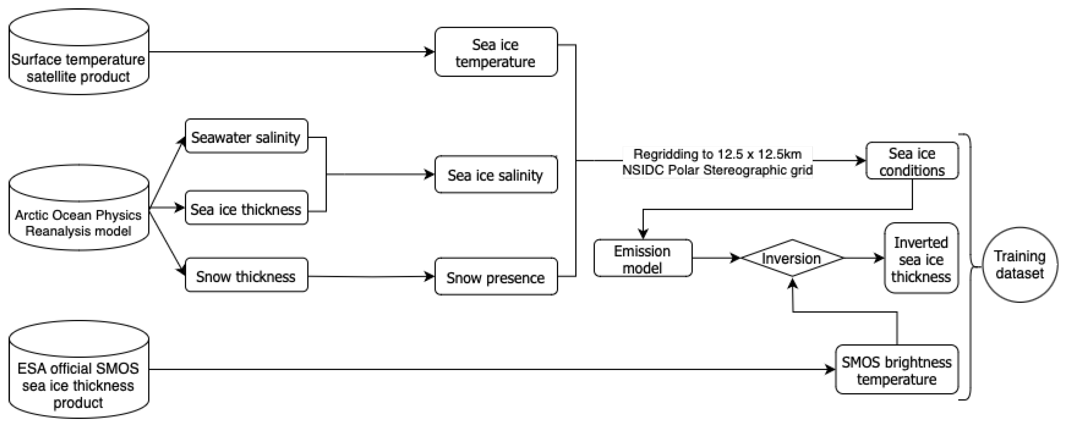
Figure 2.
Arctic-wide and Barents Sea-focused maps showing sea ice thickness estimates from each algorithm: ESA, RF, CNN, and LSTM. The Arctic-wide map corresponds to December 1st, 2019, while the Barents Sea-focused map represents the average over the campaign period, conducted from March 19th to 24th, 2014. Red stars indicate the locations of BGEP moorings in the Arctic-wide maps, while the Barents Sea maps highlight the IRO2/ESA SMOSice campaign sampling area with a white perimeter.
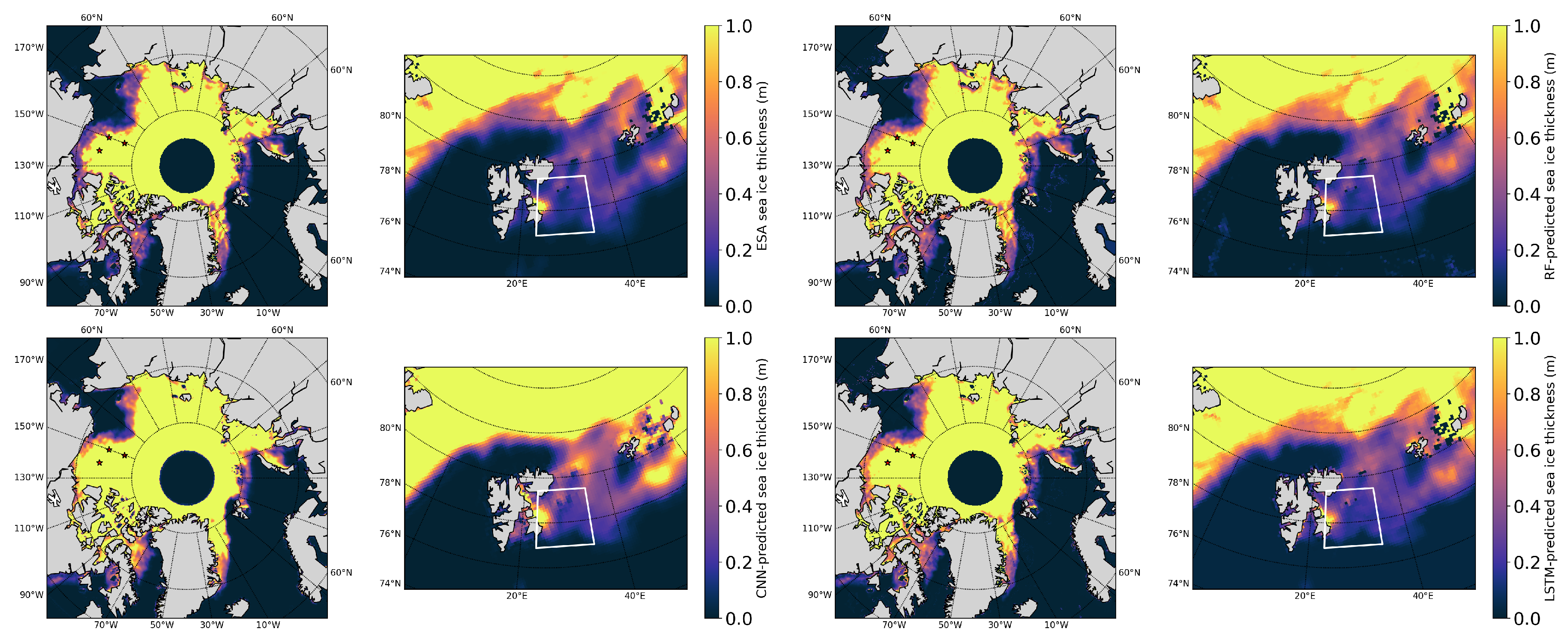
Figure 3.
Scatter and density plots of the validation of the algorithms (ESA, RF, CNN and LSTM) using the BGEP moorings dataset.
Figure 3.
Scatter and density plots of the validation of the algorithms (ESA, RF, CNN and LSTM) using the BGEP moorings dataset.
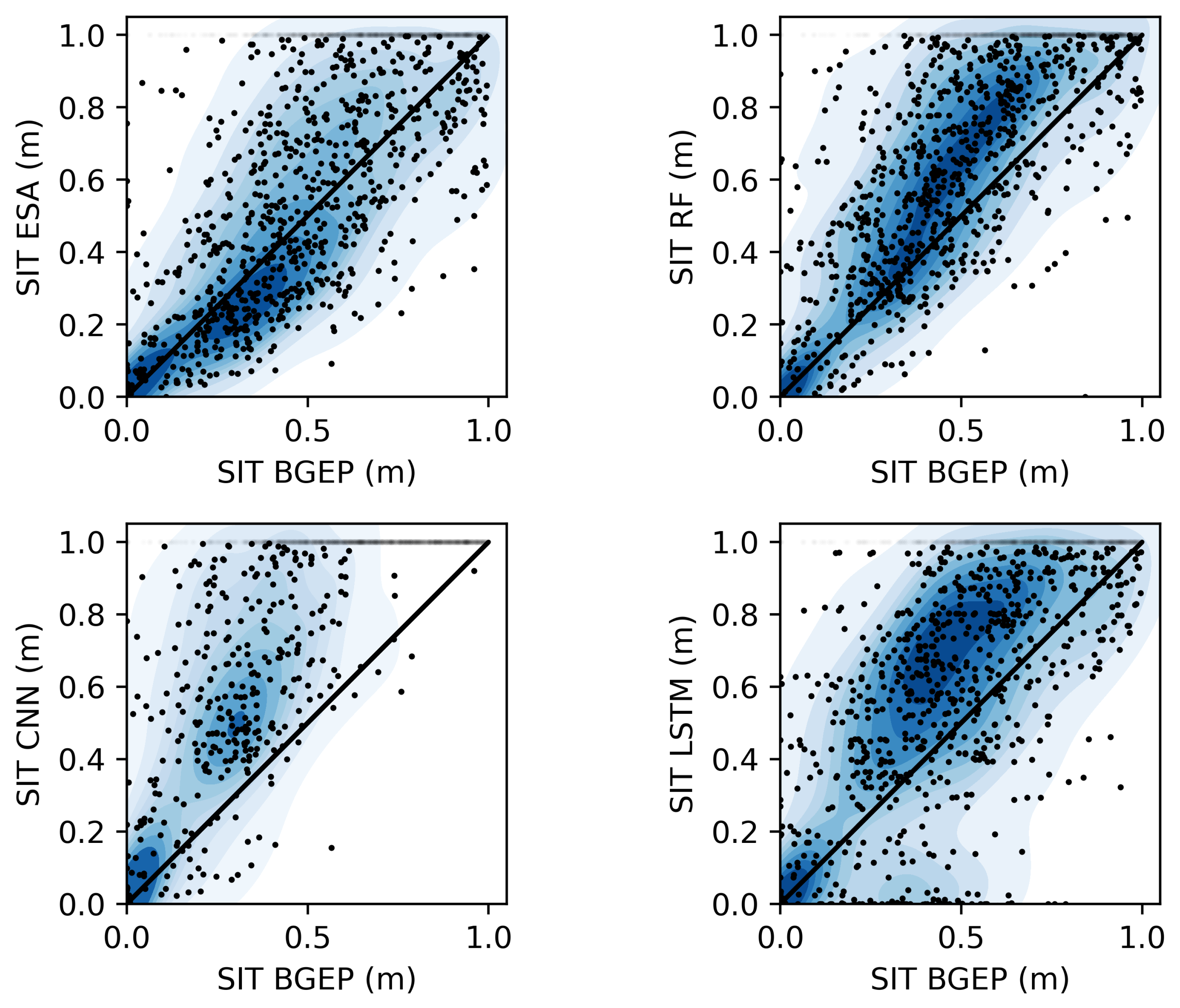
Figure 4.
Scatter and density plots of the validation of the algorithms (ESA, RF, CNN and LSTM) using the IRO2/ESA SMOSice campaign dataset.
Figure 4.
Scatter and density plots of the validation of the algorithms (ESA, RF, CNN and LSTM) using the IRO2/ESA SMOSice campaign dataset.
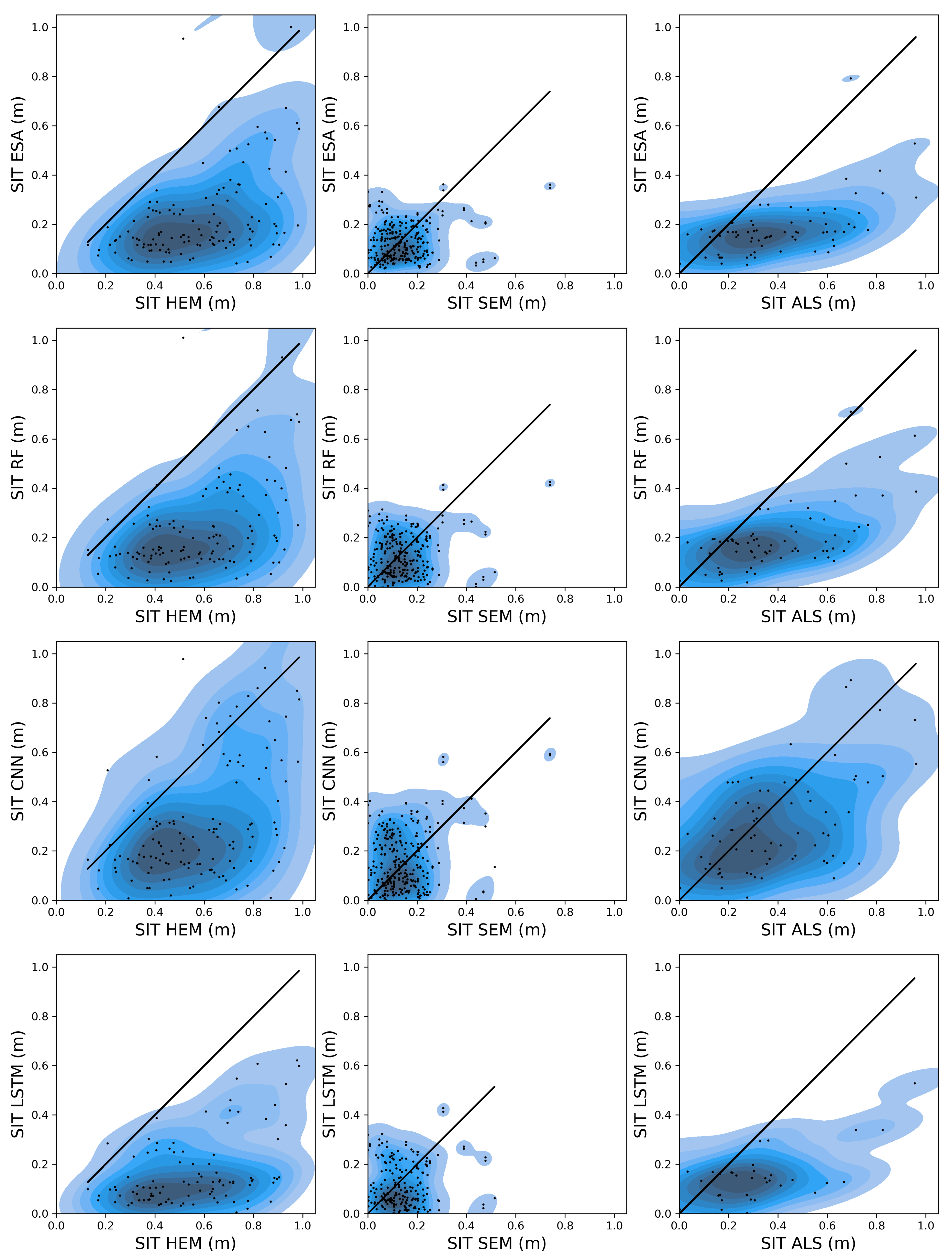
Figure 5.
Temporal evolution of the BGEP moorings (A, B, C) sea ice thickness from October 2010 to April 2021, alongside the algorithm’s prediction. The shaded part above the black solid line correspond to the values above 1 m that are not considered in the analysis.
Figure 5.
Temporal evolution of the BGEP moorings (A, B, C) sea ice thickness from October 2010 to April 2021, alongside the algorithm’s prediction. The shaded part above the black solid line correspond to the values above 1 m that are not considered in the analysis.
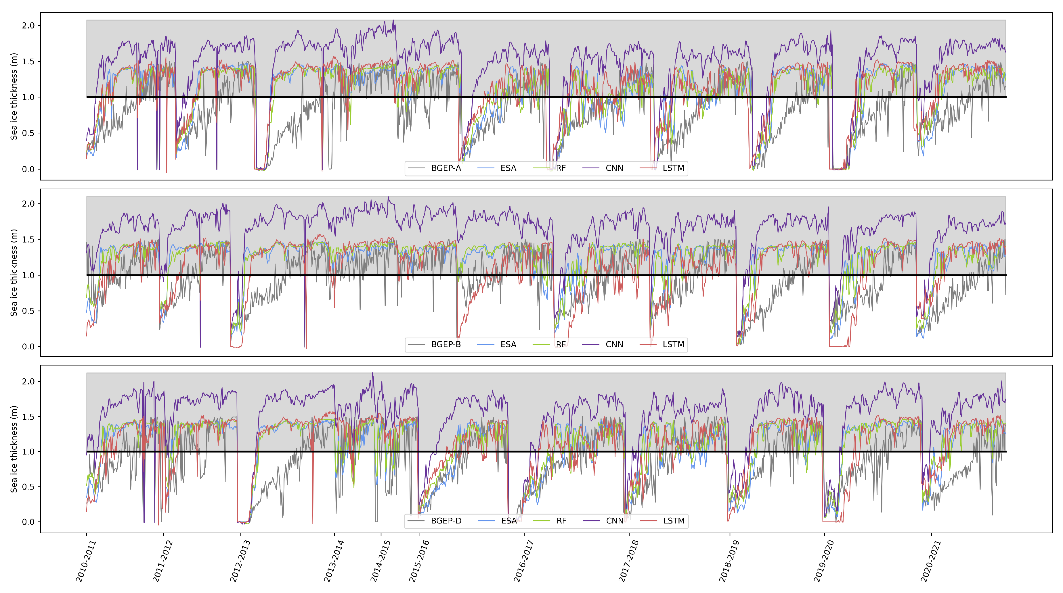
Table 1.
Layers of the Convolutional Neural Network (CNN) designed for the spatial-coherence approach.
Table 1.
Layers of the Convolutional Neural Network (CNN) designed for the spatial-coherence approach.
| Layer | Operation | Filters | Kernel | Activation |
|---|---|---|---|---|
| 1 | Convolution | 6 | (3 3) | ReLu |
| 2 | Convolution | 12 | (3 3) | ReLu |
| 3 | Convolution | 12 | (3 3) | ReLu |
| 4 | Convolution | 12 | (3 3) | ReLu |
| 5 | Convolution | 12 | (3 3) | ReLu |
| 6 | Convolution | 24 | (3 3) | ReLu |
| 7 | Convolution | 1 | (3 3) | Linear |
Table 3.
Metrics of the validation of the algorithms (ESA, RF, CNN and LSTM) using the BGEP moorings dataset.
Table 3.
Metrics of the validation of the algorithms (ESA, RF, CNN and LSTM) using the BGEP moorings dataset.
| Algorithm | R2 | MAE (m) | Std Dev (m) | overestimation (%) | underestimation (%) |
|---|---|---|---|---|---|
| ESA | 0.70 | 0.24 | 0.33 | 43.04 | 10.68 |
| RF | 0.73 | 0.24 | 0.30 | 48.76 | 4.71 |
| CNN | 0.67 | 0.30 | 0.26 | 62.58 | 1.11 |
| LSTM | 0.67 | 0.25 | 0.33 | 53.17 | 6.23 |
Table 4.
Metrics of the validation of the algorithms (ESA, RF, CNN and LSTM) using the IRO2/ESA SMOSice campaign datasets, namely HEM, SEM and ALS data.
Table 4.
Metrics of the validation of the algorithms (ESA, RF, CNN and LSTM) using the IRO2/ESA SMOSice campaign datasets, namely HEM, SEM and ALS data.
| Algorithm | R2 | MAE (m) | Std Dev (m) | overestimation (%) | underestimation (%) |
|---|---|---|---|---|---|
| HEM | |||||
| ESA | 0.49 | 0.36 | 0.22 | 1.50 | 92.48 |
| RF | 0.48 | 0.36 | 0.22 | 1.50 | 90.23 |
| CNN | 0.51 | 0.30 | 0.28 | 3.01 | 78.20 |
| LSTM | 0.43 | 0.39 | 0.14 | 1.01 | 96.97 |
| SEM | |||||
| ESA | 0.18 | 0.09 | 0.07 | 29.78 | 47.06 |
| RF | 0.19 | 0.10 | 0.09 | 35.66 | 43.01 |
| CNN | 0.23 | 0.11 | 0.12 | 40.44 | 39.71 |
| LSTM | 0.06 | 0.11 | 0.10 | 37.18 | 44.44 |
| ALS | |||||
| ESA | 0.52 | 0.24 | 0.11 | 17.86 | 71.43 |
| RF | 0.57 | 0.22 | 0.12 | 20.24 | 69.05 |
| CNN | 0.45 | 0.20 | 0.19 | 32.14 | 45.24 |
| LSTM | 0.59 | 0.19 | 0.10 | 20.51 | 64.10 |
Disclaimer/Publisher’s Note: The statements, opinions and data contained in all publications are solely those of the individual author(s) and contributor(s) and not of MDPI and/or the editor(s). MDPI and/or the editor(s) disclaim responsibility for any injury to people or property resulting from any ideas, methods, instructions or products referred to in the content. |
© 2025 by the authors. Licensee MDPI, Basel, Switzerland. This article is an open access article distributed under the terms and conditions of the Creative Commons Attribution (CC BY) license (http://creativecommons.org/licenses/by/4.0/).
Copyright: This open access article is published under a Creative Commons CC BY 4.0 license, which permit the free download, distribution, and reuse, provided that the author and preprint are cited in any reuse.


