
Submitted:
25 July 2025
Posted:
25 July 2025
You are already at the latest version
Abstract
The escalating impacts of climate change necessitate enhanced monitoring techniques for debris covered glaciers (DCG) , a critical yet challenging subject in environmental studies. This urgency underscores the importance of developing advanced methodologies that improve precision in satellite imagery analysis. Our study introduces the Physics-Informed cascaded Swin-Unet (PICSw-UNet) model, a substantial upgrade over traditional segmentation methods such as UNet-ResNet34. By integrating domain-specific physical knowledge with deep learning, our model refines segmentation tasks effectively. Leveraging the architecture of Swin-UNet cascades, this hybrid approach incorporates physical constraints into the training process, guiding the learning algorithm towards more realistic and accurate predictions. Experimental results demonstrate the superiority of our model with improvements in key performance metrics, including Intersection over Union (IoU) and Area Under the Curve (AUC). Specifically, the Physics-Informed cascaded Swin-Unet (PICSw-UNet) achieved an IoU of 91.65\% and an AUC of 96.4\%, compared to 81.24\% and 87.6\%, respectively, for the UNet-ResNet34. Moreover, our model also shows enhanced efficiency with a reduced inference time (IT) of 0.2795 seconds. These advancements indicate promising implications for future remote sensing applications and glaciological studies, offering a promising direction for advancing image analysis methodologies.
Keywords:
debris covered glaciers
; Glacial ice segmentation
; Satellite imagery analysis
; Deep learning
; Swin-UNet
; Physics-informed modeling
; Glacier monitoring
; Image segmentation techniques
1. Introduction
Glacier studies are essential for understanding Earth’s climate and its impacts, with a specific focus on debris ice detection within glaciers. Debris ice, formed by accumulated debris on glacier surfaces, significantly alters glacier behavior, influencing flow dynamics and melting patterns. Detecting debris ice is crucial for assessing glacier health and stability, which in turn informs predictions regarding water resource availability, sea-level rise and natural hazard assessments in glacierized regions. Additionally, insights gained from studying debris ice contribute to refining climate models and enhancing understanding of glacier response to climate change. Thus, comprehensive glacier studies, including debris ice detection, are fundamental for informed decision-making and effective mitigation strategies in response to ongoing climate challenges.
Recent assessments of Himalayan glaciers project a loss of up to 75% of their ice by 2100 under current warming trends. This prospective reduction in glacier volume poses a dire threat to the availability of freshwater for nearly two billion people residing in, or dependent on, the waters flowing from the Himalayan region. Additionally, the Swiss glaciers have exhibited unprecedented rates of melt, with a reduction of 10% in volume within just the past two years, highlighting the rapid impacts of climate change [1].
The accelerating rate of glacier melt affects various critical aspects of human life and the environment. It contributes to rising sea levels, which threaten coastal communities and ecosystems. The diminishing glacier mass also jeopardizes the availability of freshwater resources essential for irrigation, drinking and hydropower generation, impacting millions who rely on glacier-fed rivers for their livelihood. Furthermore, changes in glacier dynamics can disrupt ecosystems and biodiversity, affecting flora, fauna and the services these ecosystems provide. The presence of debris significantly affects how glaciers respond to climate change, creating diverse patterns in glacier behavior [2,3,4,5,6,7]. Accurately determining the extent and thickness of supraglacial debris is crucial for glacio-hydrologic models [7,8,9,10,11]. Neglecting the presence of debris cover can result in errors in estimating glacial retreat rates, mass loss and the longevity of glacial water resources. Current global supraglacial debris databases, such as the Randolph Glacier Inventory, suffer from limitations due to their reliance on heterogeneous glacier inventories [12].
Recent efforts have significantly improved the understanding of DCG through the use of Synthetic Aperture Radar (SAR) and optical imaging techniques [13,14]. Traditional methods in glacier monitoring have historically relied on pixel-based and object-based image analysis techniques [15,16,17,18,19]. These methods have been instrumental in remote sensing image classification and entity extraction, providing foundational frameworks for glacier segmentation.
Pixel-based image analysis (PBIA) involves the evaluation and grouping of individual pixels based on statistical clustering of their values [15,16]. Object-based image analysis (OBIA) extends the segmentation process beyond individual pixels, grouping them into near-homogeneous objects based on spectral, spatial, contextual, hierarchical and textual attributes [17]. Commonly employed statistical classifiers, such as nearest neighbor or random forest and rule-based classification methods enhance the efficacy of OBIA [19].
Glacier image segmentation is a critical task in remote sensing applications for understanding glacier dynamics and monitoring changes over time. Traditional methods for glacier image segmentation have been based on various techniques, including threshold, clustering and edge detection [20,21,22,23]. While these methods have shown promise in glacier image segmentation, they often face challenges in accurately delineating glacier boundaries, especially in complex terrain and under varying environmental conditions.
In addition to optical methods, Synthetic Aperture Radar imaging plays a crucial role in glacier surface classification [24,25]. Recent studies advocate for integrating optical and SAR imaging to achieve a more comprehensive understanding of glacier dynamics [26,27,28,29,30,31]. Machine learning methods, particularly deep learning architectures, have shown promising results in various image segmentation tasks [26,27,30,31].
Existing glacier segmentation methods face several challenges that impede their accuracy and efficiency. One notable difficulty arises from the rugged and heterogeneous nature of glacier terrains, complicating the precise delineation of glacier boundaries, especially across varied environmental conditions. Moreover, the limited availability of labeled data presents a obstacle, particularly concerning machine learning approaches. Additionally, traditional methods often necessitate manual parameter adjustment and lack resilience to noise and artifacts in the imagery, further complicating segmentation. Furthermore, deploying these techniques on memory-constrained devices for on-site, real-time processing poses additional hurdles, emphasizing the necessity for more streamlined and scalable segmentation techniques to overcome these obstacles.
This work introduces several innovative contributions to remote sensing and image segmentation, with a particular focus on debris-covered glaciers (DCG). Specifically, it proposes a cascaded Swin-UNet model enhanced by physics-informed inputs. The approach incorporates thermal infrared data as an additional channel, thereby capturing the characteristic thermal properties of DCG. Although many physics-informed neural networks (PINNs) incorporate partial differential equation (PDE) constraints into their loss functions [32,33], it is also well established to embed domain knowledge by adding physically relevant features or channels to the input data [34,35,36,37,38,39]. Here, the thermal infrared band serves as a physics-informed channel, furnishing temperature-based cues that assist the model in distinguishing debris-covered from clean ice without explicit PDE terms. This practice aligns with broader physics-guided strategies in remote sensing, whereby physically meaningful variables are incorporated directly into the model pipeline to improve predictive accuracy. Consequently, the resulting hybrid method leverages fundamental glaciological insights to enhance segmentation reliability, thereby establishing a robust, physics-informed framework within deep learning for remote sensing and glaciological analysis.
- Physics-Informed Integration and Cascaded Swin-UNet Architecture: This work incorporates thermal data as a physics-informed channel in the segmentation process to leverage the distinct thermal signatures of DCG, enhancing segmentation accuracy. This is a novel application in the context of Swin-UNet architectures. Furthermore, the method employs a cascaded architecture involving two Swin-UNet models. The first model generates initial segmentation masks, which are refined by a second Swin-UNet that processes inputs augmented with thermal imaging data. This cascaded approach boosts the precision and reliability of the segmentation outputs.
- SVD-Based Weight Pruning: Furthermore, it optimize the Swin-UNet using Singular Value Decomposition (SVD) to prune the model weights. This technique reduces the model’s complexity and computational demands, facilitating deployment on platforms with limited processing capabilities while maintaining high segmentation accuracy.
- Hybrid Dice-Focal Loss Function: In addition the use of a hybrid loss function combining Dice loss and focal loss addresses class imbalance effectively. This dual approach is particularly adept at improving the model’s ability to delineate under-represented classes and enhances the overlap accuracy between predicted and actual segmentation masks.
The novelty of our approach lies in the integration of physics-informed thermal infrared data into a cascaded Swin-UNet model, which enhances the model’s ability to segment debris-covered glaciers (DCG). Unlike traditional deep learning approaches that rely solely on spectral data, our method leverages the physical signatures of surface temperature to inform segmentation. This infusion of physical insight allows the model to make more accurate predictions in complex environmental conditions, setting it apart from other techniques like UNet-ResNet34 and Swin-UNet that do not incorporate such domain-specific knowledge. This rest of the manuscript is organized as follows, introduces of the study area is given in Section 2. Section 3 details the dataset and pre-processing steps, followed by Section 4, which outlines the architecture and methodology of the PICSw-UNet model. Finally, Section 5 presents the experimental results, showcasing our model’s performance in comparison to existing methods.
2. Dataset and Data Explanation
This work derives the foundational dataset from multispectral imagery captured by the Landsat 7 satellite, launched by NASA and the U.S. Geological Survey (USGS) on April 15, 1999. The satellite is equipped with the Enhanced Thematic Mapper Plus (ETM+) sensor, which collects data across various spectral bands crucial for environmental monitoring and research, including visible, near-infrared, short-wave infrared, and thermal infrared spectra.
2.1. Location of Study Area
The study area lies within the Hindu Kush Himalaya (HKH) region, spanning geographical coordinates from 27° to 38° N latitude and 67° to 98° E longitude. The region contains glaciers critical for water supply, climate regulation, and ecological stability in countries such as Afghanistan, Bangladesh, Bhutan, China, India, Myanmar, Nepal, and Pakistan. Often called the "Third Pole," the HKH region holds the largest concentration of ice outside the polar regions, with an estimated 6000 cubic kilometers of ice. Temperatures in the HKH region vary with elevation. Higher altitudes experience temperatures below -20°C in winter, while lower elevations exceed 15°C in summer. This variation, combined with monsoon and westerly weather systems, significantly influences glacier dynamics and water availability. Debris-covered glaciers in the HKH region interact with the climate in complex ways. The debris layer, made of rocks and sediment, insulates the underlying ice and modifies melt rates. This interaction leads to differential melting, complicating predictions of glacier retreat and water release.
Figure 1.
Study Area Map.
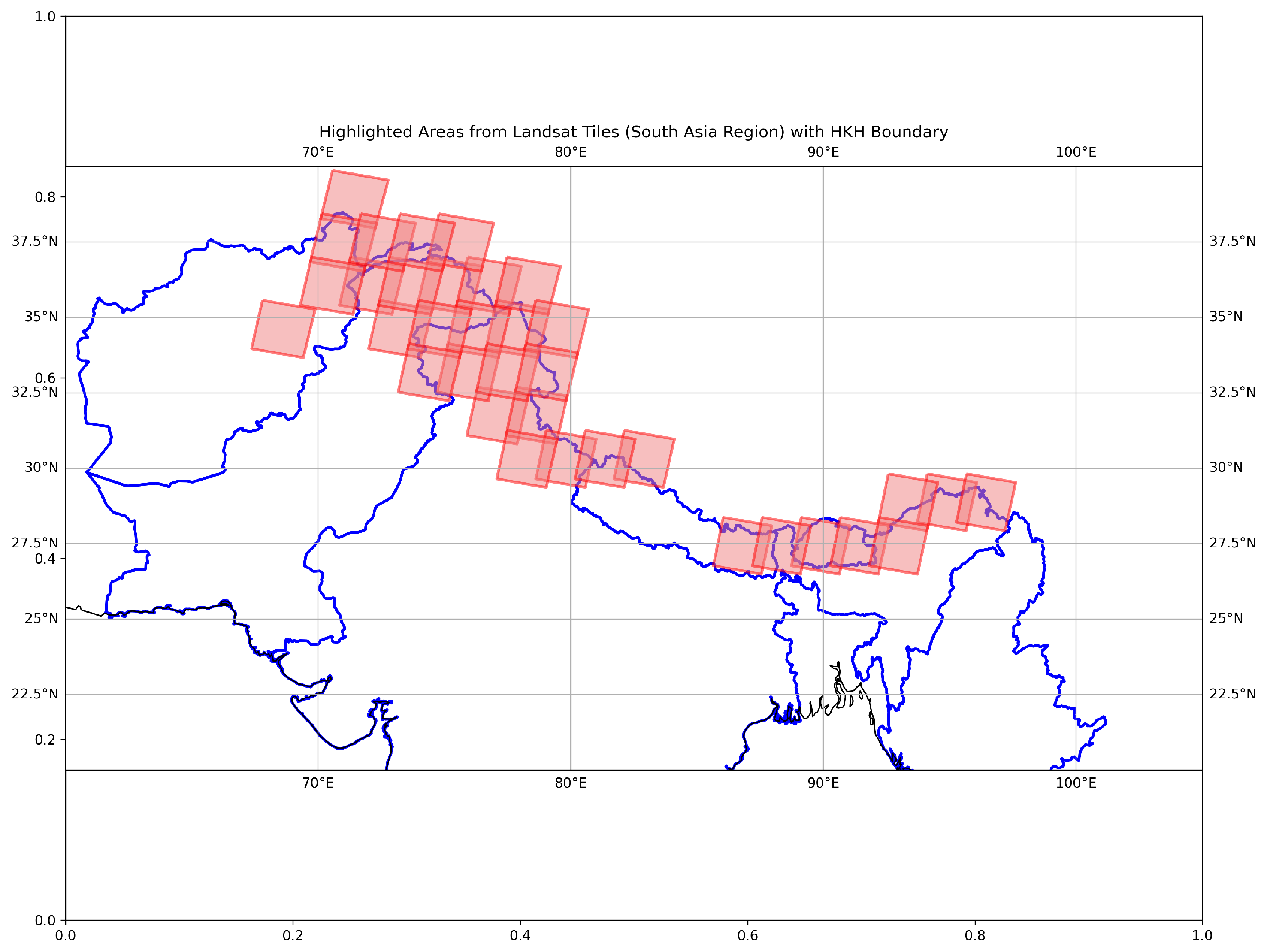
Global warming accelerates glacier melting in the HKH region, threatening freshwater reserves. The potential loss of these glaciers endangers water availability for agriculture, hydropower production, and millions of people’s livelihoods. Furthermore, the rapid glacier melting contributes to rising sea levels, posing risks to coastal communities worldwide.
2.2. Dataset Details
This work uses the HKH Glacier Mapping dataset, which includes multispectral imagery and glacier annotations from the HKH region. The dataset comprises 35 Landsat tiles, each covering an area of about 6 km x 7.5 km, with a spatial resolution of 30 meters. These tiles analyze glaciers identified and classified by the International Centre for Integrated Mountain Development (ICIMOD). The dataset includes 15 channels, each providing key information for glacier classification and analysis:
-
LE7 Bands:
- –
- B1 (Blue)
- –
- B2 (Green)
- –
- B3 (Red)
- –
- B4 (Near Infrared)
- –
- B5 (Shortwave Infrared 1)
- –
- B6_VCID_1 (Low-gain Thermal Infrared)
- –
- B6_VCID_2 (High-gain Thermal Infrared)
- –
- B7 (Shortwave Infrared 2)
- –
- B8 (Panchromatic)
- Quality Bitmask (BQA) identifies pixel quality and usability.
- Vegetation Index (NDVI)
- Snow Index (NDSI)
- Water Index (NDWI)
- SRTM 90 Elevation (upscaled from 90m to 30m)
- SRTM 90 Slope (upscaled from 90m to 30m)
Figure 2 shows an example of the image patches and their corresponding binary masks.
An existing study [40] preprocesses these original tiles to generate 7,095 image patches, each of size 512 x 512 x 15. Each patch includes a binary mask of size 512 x 512 x 2, with channels corresponding to clean ice (value 0) and debris-covered glaciers (DCG) (value 255). These patches support the training and evaluation of machine learning models for glacier mapping.
3. Swin-UNet Model Architecture
Transformer models, first introduced by Vaswani et al. [41], have revolutionized natural language processing (NLP) and are increasingly applied in diverse domains. The architecture of Transformer models, characterized by self-attention mechanisms, enables parallel processing of sequences and effective handling of long-range dependencies [42]. In computer vision and image processing, the adaptation of Transformer models has led to advancements. Vision Transformers (ViT) [43] treat images as sequences of patches, allowing for comprehensive analysis of visual data. The Swin Transformer [44], further refines this approach with a hierarchical structure and shifted window self-attention, making it particularly adept at handling tasks like image segmentation. The Swin-UNet architecture represents an innovative fusion of the Swin Transformer and the traditional U-Net framework, tailored for biomedical image segmentation. This hybrid model leverages the hierarchical structure and the shifted window self-attention mechanism of the Swin Transformer as its backbone, enhancing U-Net’s feature extraction and localization capabilities.
3.1. Integrating Swin Transformer as Backbone
The Swin Transformer processes input images in a hierarchical manner, allowing the Swin-UNet to handle features at multiple scales effectively. The architecture of Swin-UNet can be described as follows:
where I denotes the input image, represents the hierarchical feature extraction performed by the Swin Transformer and indicates the segmentation processing of U-Net utilizing these features.
Figure 3.
Architecture of Swin-UNet.
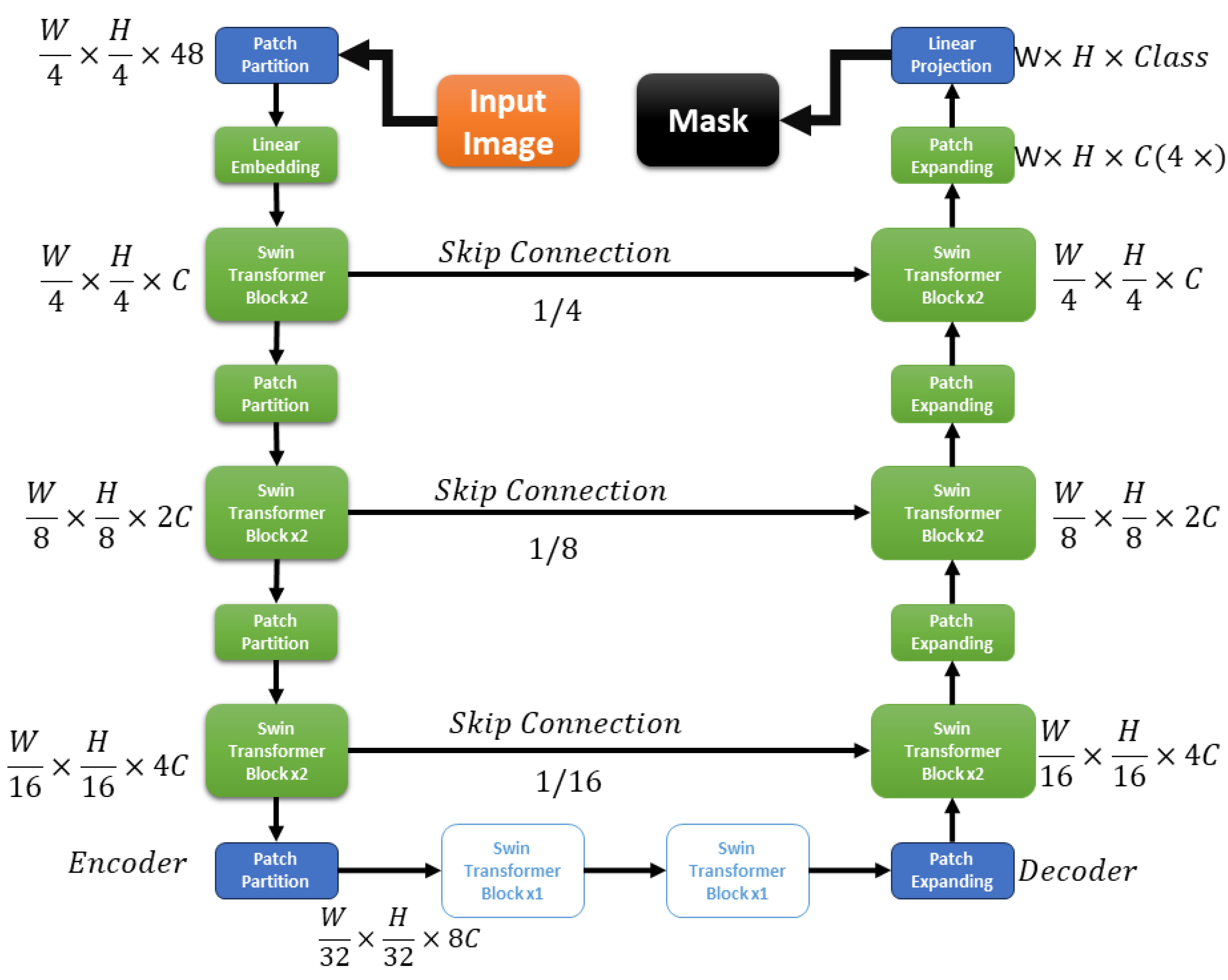
3.2. Hierarchical Feature Representation
The Swin Transformer’s hierarchical design allows for efficient processing of high-resolution images. It captures features at multiple scales, facilitating accurate segmentation. The hierarchical feature representation enables Swin-UNet to understand both global context and fine details within the image, crucial for precise segmentation.
3.3. Shifted Window Self-Attention
The Swin Transformer incorporates shifted window self-attention, which limits attention computation to non-overlapping local windows. This mechanism significantly reduces computational complexity and allows the model to focus on relevant features within each window. The Swin-UNet benefits from this attention mechanism, enabling it to process large images efficiently while maintaining segmentation accuracy.
3.4. SVD-based Optimization
Singular Value Decomposition (SVD) is a matrix factorization method that decomposes a matrix into three separate matrices: a left singular matrix, a diagonal matrix of singular values and a right singular matrix. In the context of neural networks, SVD can be used to compress model parameters by approximating the weight matrices with lower-rank matrices, thus reducing the number of parameters and model size while preserving important information.
The SVD-based optimization is a crucial step in enhancing the efficiency of the Swin-UNet model, particularly for deployment in environments with limited computational resources. By reducing the size of the weight matrices while maintaining accuracy, this technique forms an integral part of our overall segmentation strategy. With this optimization in place, we now present the proposed segmentation scheme, which builds on this foundation through a structured, multi-phase approach designed to improve the accuracy of debris-covered glacier (DCG) segmentation.
4. Proposed Segmentation Scheme
The proposed segmentation approach aims to improve DCG segmentation through a cascaded Swin-UNet model enhanced by physics-informed inputs. The proposed cascaded Swin-UNet architecture consists of two stages. The first Swin-UNet model generates an initial segmentation mask from the input data. Then, the second Swin-UNet model refines this mask by incorporating thermal infrared data, which provides additional physical insight into the temperature variations of debris-covered glaciers. This dual-phase approach improves segmentation accuracy by progressively enhancing the model’s understanding of the glaciological context. To enhance the segmentation of debris-covered glaciers, we integrate thermal infrared data, which provides unique thermal signatures revealing the insulating effects of the debris. This additional information is critical for distinguishing between clean ice and debris-covered regions, improving the model’s ability to accurately segment glacial features based on their distinct temperature profiles.
The methodology is structured into four sections. The first section discusses data pre-processing. In the second section, the Swin-UNet model is trained using focal loss and selected channels from the dataset. During the third phase, the trained model is optimized through singular value decomposition. In the final phase, a cascaded Swin-UNet model incorporates a physics-informed thermal band from the dataset to generate a predicted mask. This mask is subsequently compared with the actual mask to evaluate the results.The overall block diagram of the proposed model is shown in Figure 4.
4.1. Data Pre-Processing
In this phase, the original dataset, which has already been divided into non-overlapping window sizes of , is passed through multiple steps to enhance data representation and identify the most significant channels in the dataset for DCG prediction. A detailed discussion of each step is provided in the following subsections.
4.1.1. Initial NaN Value Replacement
Firstly, images from the dataset, which contain multiple NaN values of various patch sizes across the 15 channels, are processed to ensure data integrity. If a NaN patch is detected, the mean values of the eight neighboring pixels (N8 neighbors) of the same patch size are computed and used to replace the NaN values. This step ensures that no valuable spatial information is lost due to missing values.
where N is the number of neighboring pixels used in the computation.
4.1.2. Channel Selection Using Point-Biserial Correlation
For selecting the most relevant channels, the Point-Biserial Correlation Coefficient is employed instead of the traditional Point-Biserial correlation coefficient. While Point-Biserial correlation is effective for measuring the linear relationship between two continuous variables and is often used for feature selection, it is not suitable for scenarios where the target variable is binary. In glacier segmentation, our target variable is binary (glacier vs. non-glacier), necessitating an alternative approach. The Point-Biserial Correlation Coefficient measures the strength and direction of the association between a continuous variable and a binary variable, making it more appropriate for this context:
where and are the means of the continuous variable for the binary categories, is the standard deviation of the continuous variable and and are the sample sizes for the two categories.
4.2. Swin-UNet Model Training
After selecting the most relevant channels—specifically, the top three channels that demonstrate the highest correlation with changes in the masks—the entire dataset with selected channels is partitioned into training and testing datasets. Eighty percent of the data is designated for training the model.
The Swin-UNet architecture, previously described, employs a hybrid Dice-Focal loss function to effectively manage the imbalance prevalent in classes of the dataset. This combined loss function integrates the Dice loss, which is crucial for optimizing the overlap between the predicted and actual masks, with the focal loss, which is tailored to enhance focus on difficult, misclassified examples. The focal component of the loss is mathematically defined as in Equation (4).
where is calculated by the Equation (5).
In these equations, p represents the probability of the class with label , is a class weighting factor and is a focusing parameter. The Dice component is calculated using the formula for the Dice coefficient, enhancing the model’s ability to improve the prediction accuracy by maximizing the overlap between the predicted and true segmentations.
Additionally, the incorporation of the Diace score further enhances the model’s capability to handle class imbalance. The Diace score, similar to the Dice coefficient, measures the overlap between the predicted and actual masks but includes a factor to adjust for class imbalances. The Diace score is defined as follows:
where P is the set of predicted positives, T is the set of true positives and is a small constant to avoid division by zero.
The combined Diace-Focal loss function, which integrates the Diace score into the focal loss, is defined as:
where is a balancing factor that regulates the influence of the Diace score within the focal loss framework.
Training the model with this Diace-Focal loss function allows for an effective balance between precision in class overlap and addressing class imbalance, focusing specifically on the challenges of detecting and delineating DCG, a significantly under-represented class in the dataset. This approach ensures that both common and rare classes are accurately modeled, enhancing overall predictive accuracy. The model then progresses to the optimization phase, where further adjustments are made to enhance its performance.
4.3. SVD-Based Model Weight Pruning
A fundamental component of transformer models is the Multi-Head Attention (MHA) mechanism, which assigns attention scores to different segments of an image. This mechanism increases the size of a model, which can slow down inference time(IT) and pose challenges for deployment on edge devices where memory is limited. To address these issues, this work incorporates an SVD-based weight pruning mechanism designed to evaluate the importance of the weights in the attention matrix of the Swin Transformer blocks used in this network.
The attention mechanism in Swin Transformers can be represented by matrix A, which is derived from the query (Q), key (K) and value (V) matrices to the shifted window strategy. The attention scores in Swin Transformers are computed as follows:
where is the dimensionality of the keys and B is a relative position bias that is unique to each pair of windows in Swin Transformers, enhancing the model’s ability to preserve local information across different window configurations.
The SVD-based pruning process begins by decomposing the attention score matrix A for each head in the MHA using Singular Value Decomposition, allowing for the expression of A as:
where U and V are orthogonal matrices representing the left and right singular vectors and is a diagonal matrix containing the singular values. These singular values provide a measure of the importance of the connections in the attention matrix.
By retaining only the top k singular values—and their corresponding vectors in U and V—the complexity of A is reduced, focusing on the most significant interactions within the matrix. This reduced form, , is given by:
where , and are the truncated versions of U, and , containing only the top k components.
This pruning reduces the number of parameters and accelerates inference by focusing computational resources on the most impactful elements of the attention mechanism. This technique is especially valuable in environments with strict memory constraints, such as edge computing devices.
4.3.1. Proof of Optimality of Weights Extracted by SVD
The optimality of the truncated Singular Value Decomposition (SVD) in the context of model weight pruning can be demonstrated using the Eckart-Young-Mirsky theorem. This theorem provides a foundational understanding that the best rank-k approximation to a matrix, in terms of the least squares error, is given by its SVD truncated to the first k singular values.
The theorem states:
where:
- denotes the Frobenius norm.
- is the approximation of A using the top k singular values.
- are the singular values of A.
- r is the rank of A.
Derivation: The Frobenius norm of the difference between A and its rank-k approximation can be expanded as follows:
Since is formed by keeping only the top k singular values (and corresponding singular vectors), it holds that and thus:
This derivation shows that is indeed the optimal rank-k approximation of A under the Frobenius norm criterion, thereby justifying the use of SVD-based pruning to maintain model performance while reducing computational requirements.
4.4. Cascaded Swin-UNet Model
In this work the existing data is given to the already trained and optimized swin-unet model let’s denote the output from the Swin-UNet model as O, which consists of two channels:
where represents the channel for clean ice and represents the channel for DCG. Each channel is a two-dimensional matrix corresponding to the spatial dimensions of the input images.
The thermal band, denoted as T, is a single-channel image of the same spatial dimensions as O. This thermal band is selected for its capability to reflect thermal variations indicative of different material properties on the ice surface, particularly highlighting areas with debris due to their typically higher temperatures from lower albedo.
The concatenation operation integrates the model outputs with the thermal data and is mathematically represented as:
This operation merges the spatial and contextual information provided by the Swin-UNet with the thermal insights from the physics-informed thermal band. The resulting image, now enriched with both visual and thermal cues, significantly enhances the model’s ability to generalize across different conditions and datasets. This composite image serves as the input for subsequent processing stages aimed at refining and enhancing the segmentation accuracy further. Algorithm 1.
| Algorithm 1 Proposed Model for Debris Ice Segmentation |
|
The newly formed images from Equation (19) serve as input to another Swin-UNet model. This second model is specifically trained on these images, learning to refine the segmentation masks further. The combination of the thermal band with outputs from the first model substantively improves segmentation accuracy, as it provides additional contextual information relevant to the physical properties of the ice.The pseudo code of proposed scheme is shown in Table 1.

Table 1.
Distribution of Sub-Images Across the Dataset Subsets.
| Subset | Original Images | Sub-Images per Image | Total Sub-Images |
|---|---|---|---|
| Training Set | 5676 | 1089 | 6,172,764 |
| Testing Set | 1064 | 1089 | 1,158,576 |
| Validation Set | 355 | 1089 | 386,595 |
5. Experiment
This section details the results of the proposed segmentation scheme. Initially, the comparison metrics are defined. Then the results of the first phase of the proposed scheme are then explored, followed by the results of the proposed cascaded Swin-UNet model are presented. Then the results of the proposed scheme are compared with other models.
5.1. Comparison Metrics
The performance of the segmentation model is evaluated using several metrics designed to provide a comprehensive assessment of its effectiveness. These metrics include Accuracy, F1 Score, Precision, Recall, Intersection over Union (IoU) and Area Under the Curve (AUC). Below, each metric is defined and explained:
- (1)
- Accuracy: This metric measures the proportion of true results (both true positives and true negatives) among the total number of cases examined. It is defined as:
- (2)
- F1 Score: The harmonic mean of Precision and Recall, the F1 Score provides a balance between them, particularly useful when dealing with an uneven class distribution. It is defined as:
- (3)
- Precision: Also known as positive predictive value, Precision measures the accuracy of positive predictions made by the model. It is computed as:
- (4)
- Recall: Also known as sensitivity, Recall indicates the ability of the model to identify all relevant instances. It is calculated as:
- (5)
- Intersection over Union (IoU): Also known as the Jaccard index, IoU measures the overlap between the predicted segmentation and the ground truth. It is defined as:
- (6)
- Area Under the Curve (AUC): Refers to the area under the Receiver Operating Characteristic (ROC) curve. It quantifies the overall ability of the model to discriminate between the classes across all thresholds. A higher AUC value indicates better model performance.
5.2. Experimental Setup
This work takes the existing dataset used in [40] ,which contains a total of 7095 images and their corresponding masks. Each image has dimensions of , and each mask has dimensions of . The dataset is divided into three subsets: training, testing, and validation, with distributions of 80%, 15%, and 5%, respectively. Therefore, the number of images in each subset is calculated as follows: the training set contains 5676 images, the testing set contains 1064 images, and the validation set contains 355 images. Next, a sliding window operation is applied to each image. The window size is , and it slides over the image in steps of 12 rows and 12 columns, resulting in 1089 overlapping sub-images for each image. Consequently, each original image and its corresponding mask are divided into 1089 sub-images. This results in the total number of sub-images for the training, testing, and validation sets being calculated based on the number of images in each subset. The distribution of sub-images across these subsets is summarized in the following Table 1.
Thus, the total number of sub-images across all subsets is 7,717,935. This setup ensures effective training and evaluation, utilizing Landsat 7’s spectral capabilities and segmentation techniques. With this foundation in place, next section disscuss focus to the Transformer models that drive our segmentation approach.
5.3. pre-Processing Results
In the implemented scheme, the dataset initially contains NaN values. These are addressed by replacing them with the mean of adjacent pixels. Subsequently, a correlation test is conducted to determine the most significant channels within the dataset for debris ice segmentation. The analysis identifies key channels that notably impact glacier segmentation: NDWI (water index), NDSI(Normalized Difference Snow Index) and LE7 B1 (Blue) channels. These channels are then chosen for constructing the input images for the model, effectively reducing the input dimensionality to . The results of the correlation tests are depicted in Figure 5.
5.4. Results of Proposed Model
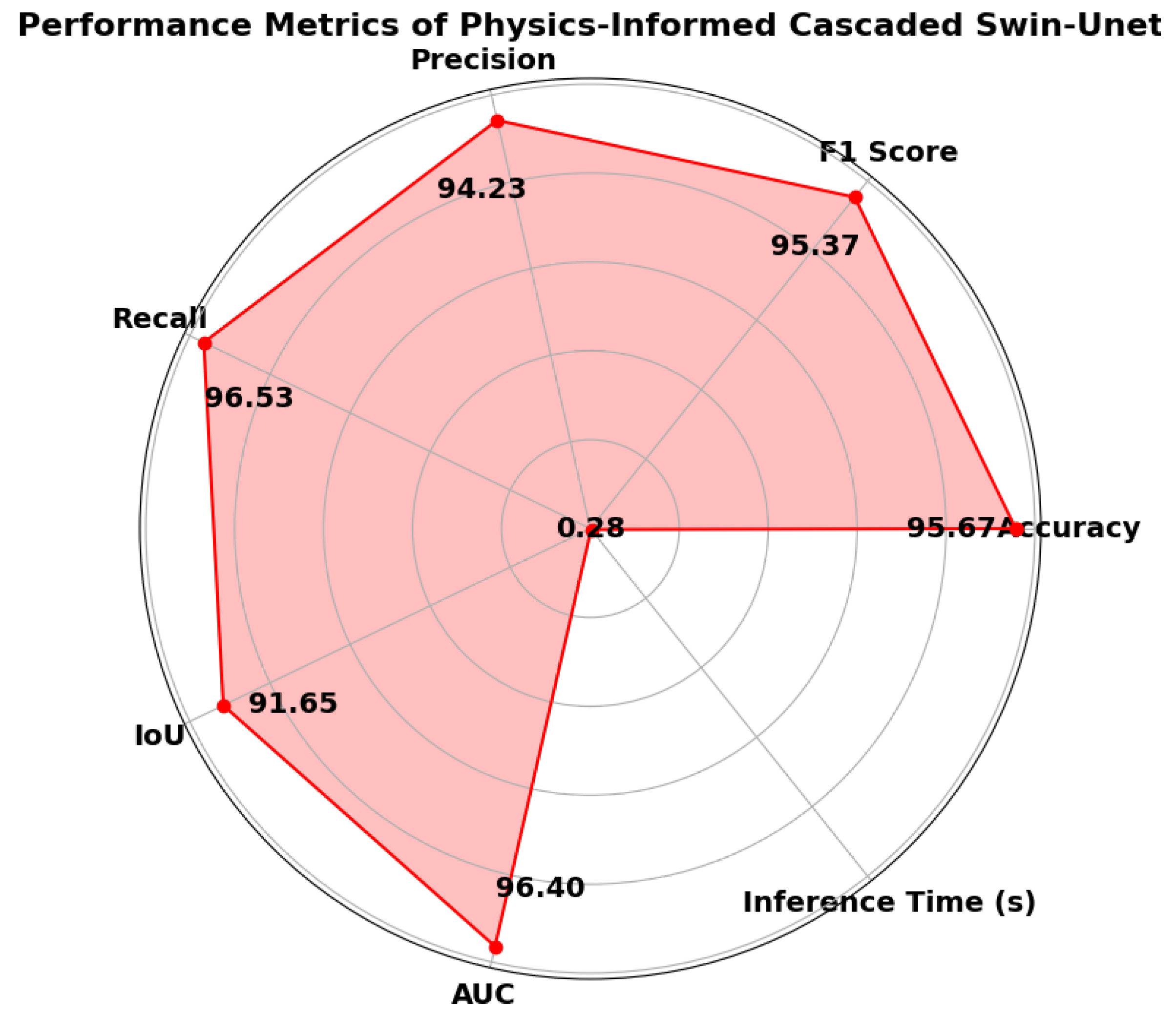
This section presents the performance results of the PICSw-UNet model, highlighting its effectiveness in debris ice segmentation tasks. The model’s metrics are visualized in a radar chart shown in Figure 7, which allows for an immediate and intuitive comparison across various critical performance measures.
The model’s Accuracy (95.67%) indicates a high level of overall correctness across all classes, which is essential for reliable predictions in real-world applications. High accuracy signifies that the model is capable of correctly classifying most of the pixels in the input images, whether they belong to DCG or clean ice. This is particularly important in environmental monitoring, where accurate segmentation can inform critical decisions and interventions.
The F1 Score (95.37%) balances precision and recall, providing a comprehensive view of the model’s ability to accurately classify debris without mis classifying clean ice. The F1 score is crucial in scenarios where both false positives (mis classifying clean ice as debris) and false negatives (missing actual debris) can have significant implications. A high F1 score demonstrates that the model maintains a good balance between precision and recall, effectively minimizing both types of errors.
Precision (94.23%) highlights the model’s capability to correctly label actual debris, which is crucial in scenarios where false positives are costly. Precision is particularly important in environmental monitoring and disaster response, where incorrectly identifying clean ice as debris could lead to unnecessary actions or missed opportunities for intervention. High precision ensures that when the model identifies debris, it is likely to be correct.
Recall (96.53%) demonstrates the model’s effectiveness in identifying all actual debris instances, vital for environmental monitoring to ensure no DCG is missed. Recall is critical in ensuring that all areas of concern are accurately detected. High recall indicates that the model successfully identifies most, if not all, of the DCG areas, which is essential for comprehensive monitoring and analysis.
The IoU (Intersection over Union) (91.65%) represents the accuracy of overlap between predicted and actual debris regions, which is important for precise segmentation. IoU is a measure of the model’s ability to predict the exact boundaries of debris-covered areas. A high IoU indicates that the predicted segmentation closely matches the ground truth, which is vital for applications requiring precise delineation of DCG.
AUC (Area Under the Curve) (96.4%) shows the model’s discriminative power, indicative of robustness against varying operational thresholds. A high AUC value indicates that the model is capable of distinguishing between DCG and clean ice across a range of threshold settings. This robustness is important for adapting the model to different operational conditions and ensuring consistent performance.
Lastly, the IT (0.2795 seconds) is critical for evaluating the model’s efficiency, particularly in time-sensitive applications. Low IT ensures that the model can process and analyze images quickly, which is crucial for real-time monitoring and decision-making scenarios. Efficient IT allows the model to be deployed in operational environments where timely information is essential.
The visual results of the proposed scheme are shown in Figure 6, providing a clear representation of the model’s segmentation capabilities. These visualizations help in understanding how well the model performs in distinguishing between debris-covered and clean ice.
The visual results shown in Figure 7 illustrate the practical effectiveness of the PICSw-UNet model. Each row, from top to bottom, showcases the input image, the original mask, the prediction by the model and the analysis of correct classifications. The clear separation between debris-covered and clean ice regions demonstrates the model’s high precision and recall. The legend helps in interpreting the different classifications, providing a comprehensive view of the model’s performance in real-world scenarios.In some instances, false positives (FP) occurred in regions where debris features closely resembled clean ice, particularly in areas with light haze or shadow. Similarly, false negatives (FN) were observed in regions with sparse debris coverage or minimal thermal contrast, where the model struggled to distinguish between clean ice and small debris patches. These errors highlight the need for further refinement in model sensitivity to subtle environmental features. In summary, the PICSw-UNet model demonstrates significant improvements in segmentation accuracy and efficiency. The high values of accuracy, F1 score, precision, recall, IoU and AUC, combined with a low IT, highlight the model’s effectiveness and practicality for real-world applications. These results underscore the model’s potential to enhance DCG segmentation, providing more accurate and reliable data for environmental monitoring and analysis.
Figure 7.
Radar Chart of the PICSw-UNet Performance Metrics.
6. Results and Discussion
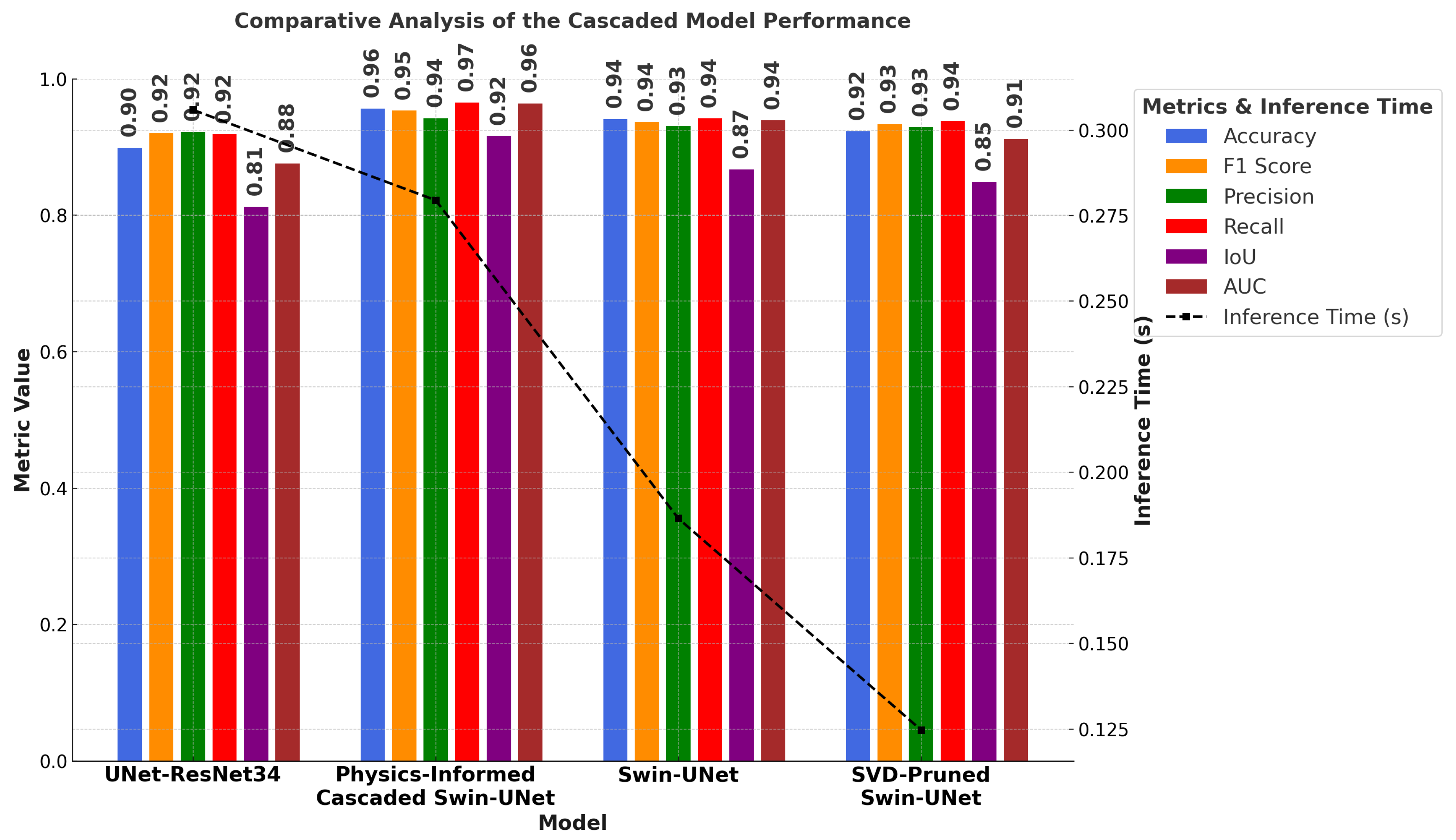
The performance of the PICSw-UNet is compared against three other models: Swin-UNet, svd-pruned swin-unet (SPSW-UNet) and UNet-ResNet34, as shown in Table 2. This comparative analysis aims to highlight the enhancements achieved by integrating physics-informed strategies into the cascaded model. The PICSw-UNet model demonstrates substantial improvements across several key performance metrics when compared to conventional models such as Swin-UNet, SPSW-UNet and UNet-ResNet34.
The model’s accuracy of 95.67% is a significant improvement over the Swin-UNet (94.12%), SPSW-UNet (92.34%) and UNet-ResNet34 (89.9%). This high level of accuracy indicates that the PICSw-UNet model can correctly classify a large proportion of the pixels in the input images, reducing the overall error rate. High accuracy is crucial in environmental monitoring where precise data interpretation is necessary for effective decision-making.
The F1 score of 95.37% for the PICSw-UNet surpasses that of the Swin-UNet (93.65%), SPSW-UNet (93.35%) and UNet-ResNet34 (92.05%). The F1 score balances precision and recall, making it a reliable metric for assessing the model’s performance, especially in scenarios with imbalanced class distributions. This high F1 score demonstrates that the proposed model can accurately identify DCG while minimizing both false positives and false negatives.
Precision measures the model’s ability to correctly identify debris without misclassifying clean ice. The PICSw-UNet achieves a precision of 94.23%, which is higher than the Swin-UNet (93.09%), SPSW-UNet (92.92%) and UNet-ResNet34 (92.2%). High precision is essential in applications where false positives can lead to unnecessary interventions or actions and this improvement underscores the model’s capability to make accurate predictions regarding DCG.
Recall for the PICSw-UNet is 96.53%, outperforming the Swin-UNet (94.21%), SPSW-UNet (93.80%) and UNet-ResNet34 (91.91%). Recall is crucial for ensuring that the model detects as many true positive instances of DCG as possible. High recall indicates that the model is effective in identifying all relevant instances, reducing the risk of overlooking areas that require monitoring or intervention.
Intersection over Union (IoU) is a metric used to evaluate the accuracy of segmentation by measuring the overlap between the predicted and actual debris regions. The PICSw-UNet achieves an IoU of 91.65%, significantly higher than the Swin-UNet (86.73%), SPSW-UNet (84.89%) and UNet-ResNet34 (81.24%). A higher IoU indicates better segmentation accuracy, which is crucial for precise delineation of DCG.
The Area Under the Curve (AUC) of the PICSw-UNet is 96.4%, higher than the Swin-UNet (93.93%), SPSW-UNet (91.20%) and UNet-ResNet34 (87.6%). A higher AUC indicates better discriminative power of the model across various threshold settings. This robustness is important for adapting the model to different operational conditions and ensuring consistent performance.
The IT for the PICSw-UNet is 0.2795 seconds, which is slower compared to Swin-UNet (0.1865 seconds) and SPSW-UNet (0.1247 seconds) but faster than UNet-ResNet34 (0.3059 seconds). While the increased IT is a drawback, it is a reasonable trade-off given the substantial improvements in other performance metrics. The slight increase in IT is justified by the model’s enhanced accuracy and robustness, making it suitable for applications where precision is more critical than speed.
The PICSw-UNet model exhibits significant improvements over traditional and SVD-pruned models. From the Swin-UNet, there is an improvement of +1.65% in accuracy, +1.84% in F1 score, +1.2% in precision, +2.46% in recall, +5.67% in IoU, +2.63% in AUC and a slower inference by 49.87%. Comparatively, against the SPSW-UNet, it shows +3.61% better accuracy, +2.16% in F1 score, +1.41% in precision, +2.91% in recall, +7.96% in IoU, +5.70% in AUC and a significant increase in IT by 124.14%. Moreover, improvements over the UNet-ResNet34 are even more pronounced with +6.42% in accuracy, +3.61% in F1 score, +2.20% in precision, +5.03% in recall, +12.81% in IoU, +10.05% in AUC and a reduction in IT by 8.63%, indicating a notable enhancement in both performance and efficiency. The inclusion of the thermal infrared channel significantly contributed to these improvements, as it allows the model to better capture the distinct thermal signatures of debris-covered glaciers (DCG). This thermal information helped the model distinguish between clean ice and debris-covered regions with greater accuracy. For instance, the model’s Intersection over Union (IoU) improved by 5.67%, and Area Under the Curve (AUC) increased by 2.63%, highlighting the contribution of the thermal data to the enhanced segmentation precision. These results indicate that incorporating thermal data as a physics-informed feature plays a critical role in refining the model’s predictions, particularly in environments where temperature variations are key to class differentiation.
The advancements underscore the model’s robustness and the efficacy of incorporating physics-informed insights to substantially elevate segmentation accuracy and operational efficiency. The pronounced improvements in key performance metrics such as Intersection over Union (IoU) and Area Under the Curve (AUC) specifically illustrate the model’s enhanced ability to distinguish between different classes more distinctly and handle complex segmentation tasks with greater precision. This indicates a significant step forward in the model’s design, where the integration of physical principles directly contributes to its computational intelligence, enabling more nuanced and accurate predictions.
The PICSw-UNet model significantly surpasses both traditional and SPSW-UNet models across all evaluated metrics, with notable advancements in IoU and AUC, metrics that are critical for assessing the precision and efficacy of segmentation tasks. These improvements are crucial for applications that rely on the accurate categorization and segmentation of images, such as environmental monitoring and glaciological studies, where precision in interpreting satellite imagery can directly impact the quality of subsequent analyses and decisions. The model demonstrates remarkable gains in accuracy, which reflects the overall correctness of the model across all test scenarios. The F1 score, which balances the precision and recall, underscores the model’s ability to correctly classify and recall instances of debris and clean ice without significant errors, providing a more reliable and consistent performance. These metrics highlight not only the model’s accuracy but also its practical effectiveness in real-world applications.
While the increase in IT, compared to both the original and the SVD-pruned models, is noticeable, it is reasonable given the substantial enhancements in model performance. This trade-off is considered acceptable in many advanced applications where the stakes of decision-making and the cost of errors are high. Furthermore, the PICSw-UNet model shows improved IT compared to the UNet-ResNet34 model, indicating its enhanced efficiency in processing despite the higher complexity. This is particularly advantageous in resource-limited scenarios where computational efficiency is as critical as accuracy.
Figure 8.
Graphical Representation of Comparative Analysis.
This detailed comparative analysis confirms the benefits of integrating physics-informed modifications into deep learning frameworks. It highlights the model’s potential to transform the field of environmental monitoring. By incorporating physical laws into the training process, the model gains an intrinsic understanding of natural phenomena, enabling it to perform with high reliability under varied and challenging conditions. This approach is essential in the field of remote sensing, where accurate data interpretation is pivotal for environmental conservation and disaster management strategies.
In short, these enhancements contribute to a robust, reliable and efficient model capable of performing complex segmentation tasks crucial for scientific research and practical applications in various fields, particularly those involving environmental studies and climate monitoring. The PICSw-UNet model represents a significant advancement in the use of machine learning to address and interpret natural phenomena, setting a new benchmark for future developments in the field.
7. Conclusions
The presented study introduces the PICSw-UNet model, advancing glacier segmentation techniques. By integrating domain-specific physical knowledge with a deep learning framework, our model achieves better performance metrics in segmenting DCG from satellite imagery. The evaluation of our model against traditional segmentation methods, such as Swin-UNet, SPSW-UNet and UNet-ResNet34, shows its effectiveness and robustness. Key performance metrics, including accuracy (95.67%), F1 score (95.37%), precision (94.23%), recall (96.53%), Intersection over Union (91.65%) and Area Under the Curve (96.4%), show improvements over the baseline models. Specifically, the PICSw-UNet shows an IoU and AUC, indicating its ability to delineate and accurately classify DCG. Although the model incurs a slightly higher IT (0.2795 seconds), this is a reasonable trade-off considering the gains in segmentation precision and accuracy. This study has many contributions, advancing glacier segmentation and offering a scalable solution for environmental monitoring and glaciological studies. The precision and reliability of the PICSw-UNet model provide insights into glacier dynamics, crucial for understanding climate change impacts and informing mitigation strategies. In conclusion, this study shows the potential of integrating physics-informed modeling with deep learning architectures to achieve improvements in complex environmental segmentation tasks. The findings highlight the importance of interdisciplinary approaches in enhancing the accuracy and efficiency of remote sensing applications, paving the way for future research and development in this area.
Supplementary Materials
The following supporting information can be downloaded at the website of this paper posted on Preprints.org, Table S1: Spectral Bands of Landsat 7 and Their Applications in Glacier Segmentation.
Author Contributions
Conceptualization, Yousaf Sardar Dasti; Methodology, Yousaf Sardar Dasti and Zhou Yushan; Software, Laeeq Aslam and Fatima Yaqoob; Validation, Zhou Yushan and Yunsheng Zhang; Data Curation, Syed Akram; Writing—Original Draft Preparation, Yousaf Sardar Dasti; Writing—Review and Editing, Fatima Yaqoob and Zhou Yushan; Supervision, Zhou Yushan and Yunsheng Zhang. All authors have read and agreed to the published version of the manuscript.
Funding
This work was partially supported by the Science and Technology Research and Development Program Project of China Railway Group Limited (Major Special Project, No.: 2021-Special-08) whereas another part was supported by the Hunan Provincial Natural Science Foundation of China (grant number: 2024JJ6497).
Conflicts of Interest
The authors declare no conflict of interest.
References
- Deutsche Welle. Swiss Glaciers Record Unprecedented Melt Rates. https://www.dw.com/en/swiss-glaciers-melt/a-57483958, 2023. Accessed: 2024-04-24.
- Sakai, A.; Fujita, K. Contrasting glacier responses to recent climate change in high-mountain Asia. Scientific Reports 2017, 7, 13717. [Google Scholar] [CrossRef]
- Quincey, D.J.; Glasser, N.F. Morphological and ice-dynamical changes on the tasman glacier, New Zealand, 1990–2007. Glob. Planet. Change 2009, 68, 185–197. [Google Scholar] [CrossRef]
- Jiang, S.; Nie, Y.; Liu, Q.; Wang, J.; Liu, L.; Hassan, J.; et al. Glacier change, supraglacial debris expansion and glacial lake evolution in the gyirong river basin, central Himalayas, between 1988 and 2015. Remote Sens. 2018, 10, 986. [Google Scholar] [CrossRef]
- Mölg, N.; Bolch, T.; Walter, A.; Vieli, A. Unravelling the evolution of zmuttgletscher and its debris cover since the end of the little ice age. Cryosphere 2019, 13, 1889–1909. [Google Scholar] [CrossRef]
- Tielidze, L.G.; Bolch, T.; Wheate, R.D.; Kutuzov, S.S.; Lavrentiev, I.I.; Zemp, M. Supra-glacial debris cover changes in the Greater Caucasus from 1986 to 2014. Cryosphere 2020, 14, 585–598. [Google Scholar] [CrossRef]
- Herreid, S.; Pellicciotti, F. The state of rock debris covering Earth’s glaciers. Nat. Geosci 2020, 13, 621–627. [Google Scholar] [CrossRef]
- Ragettli, S.; Immerzeel, W.W.; Pellicciotti, F. Contrasting climate change impact on river flows from high-altitude catchments in the Himalayan and Andes Mountains. Proc. Natl. Acad. Sci. U. S. A. 2016, 113, 9222–9227. [Google Scholar] [CrossRef]
- Rounce, D.R.; King, O.; Mccarthy, M.; Shean, D.E.; Salerno, F. Quantifying debris thickness of debris-covered glaciers in the everest region of Nepal through inversion of a subdebris melt model. J. Geophys. Res. Earth Surf. 2018, 123, 1094–1115. [Google Scholar] [CrossRef]
- Aslam, L.; Saeed, A.; Qureshi, I.M.; Amir, M.; Khan, W. Novel Image Steganography Based on Preprocessing of Secrete Messages to Attain Enhanced Data Security and Improved Payload Capacity. Traitement du Signal 2020, 37. [Google Scholar] [CrossRef]
- Aslam, L.; Zou, R.; Awan, E.S.; Hussain, S.S.; Shakil, K.A.; Wani, M.A.; Asim, M. Hardware-Centric Exploration of the Discrete Design Space in Transformer–LSTM Models for Wind Speed Prediction on Memory-Constrained Devices. Energies 2025, 18, 2153. [Google Scholar] [CrossRef]
- Racoviteanu, A.; Nicholson, L.; Glasser, N. Surface composition of debris-covered glaciers across the Himalaya using linear spectral unmixing of Landsat 8 OLI imagery. Cryosphere 2021, 15, 4557–4588. [Google Scholar] [CrossRef]
- Kulkarni, S.C.; Rege, P.P. Pixel level fusion techniques for SAR and optical images: A review. Information Fusion 2020, 59, 13–29. [Google Scholar] [CrossRef]
- Begam, S.; Sen, D. Mapping of moraine dammed glacial lakes and assessment of their areal changes in the central and eastern Himalayas using satellite data. Journal of Mountain Science 2019, 16, 77–94. [Google Scholar] [CrossRef]
- Ardelean, F.; Ginzler, C.; Gartner-Roer, I.; Götz, J. Glacier classification and mapping by object-based image analysis (OBIA), using optical data from different sensors: A case study from the Suntar-Khayata Range, Russian Siberia. Remote Sensing 2011, 3, 782–800. [Google Scholar]
- Bajracharya, S.R.; Shrestha, B.R. Automated mapping of debris-covered glaciers using object-based image analysis of Landsat data: A case study of Yala Glacier in Langtang Valley, Nepal. Geocarto International 2015, 30, 636–651. [Google Scholar]
- Karimi, F.; Bahremand, A.; Roodposhti, M.S.; et al. Detection of supraglacial lakes on debris-covered glaciers in the Himalaya/Karakoram using Landsat imagery. Journal of Applied Remote Sensing 2015, 9, 096098. [Google Scholar]
- Nie, Y.; Sheng, Y.; Wang, Y.; et al. A semi-automated object-based approach for glacier mapping. Journal of Geographical Sciences 2010, 20, 415–428. [Google Scholar]
- Rastner, P.; Bolch, T.; Notarnicola, C.; Paul, F. A comparison of pixel- and object-based glacier classification with optical satellite images. IEEE J. Sel. Top. Appl. Earth Observations Remote Sens. 2014, 7, 853–862. [Google Scholar] [CrossRef]
- Smith, J.D.; Johnson, E.F. Glacier segmentation from satellite imagery. Remote Sensing Letters 2007, 3, 307–316. [Google Scholar]
- Jones, M.A.; Smith, J.D. Comparative analysis of clustering algorithms for glacier segmentation. International Journal of Remote Sensing 2010, 31, 5417–5434. [Google Scholar]
- Johnson, E.F.; Wang, L.; Liu, W. Automated glacier boundary extraction from aerial photographs using edge detection algorithms. Photogrammetric Engineering & Remote Sensing 2015, 81, 159–169. [Google Scholar]
- Wang, L.; Liu, W. Deep glacier segmentation using convolutional neural networks. IEEE Transactions on Geoscience and Remote Sensing 2018, 56, 218–233. [Google Scholar]
- Nagai, H.; Abe, T.; Ohki, M. SAR-based flood monitoring for flatland with frequently fluctuating water surfaces: Proposal for the normalized backscatter amplitude difference index (NoBADI). Remote Sensing 2021, 13, 4136. [Google Scholar] [CrossRef]
- Muhammad, S.; Thapa, A. Daily Terra–Aqua MODIS cloud-free snow and Randolph Glacier Inventory 6.0 combined product (M* D10A1GL06) for high-mountain Asia between 2002 and 2019. Earth System Science Data 2021, 13, 767–776. [Google Scholar] [CrossRef]
- Bhardwaj, A.; et al. Synthesizing optical and SAR imagery from land cover maps and auxiliary raster data. IEEE Transactions on Geoscience and Remote Sensing 2021, 60, 1–12. [Google Scholar] [CrossRef]
- Singh, S.; et al. A sensitivity analysis on the spectral signatures of low-backscattering sea areas in Sentinel-1 SAR images. Remote Sensing 2021, 13, 1183. [Google Scholar] [CrossRef]
- Mirza, H.A.; Aslam, L.; Raja, M.A.Z.; Chaudhary, N.I.; Qureshi, I.M.; Malik, A.N. A New Computing Paradigm for Off-Grid Direction of Arrival Estimation Using Compressive Sensing. Wireless Communications and Mobile Computing 2020, 2020, 9280198. [Google Scholar] [CrossRef]
- Saeed, A.; Shahzad, E.; Aslam, L.; Qureshi, I.M.; Khan, A.U.; Iqbal, M. A New Paradigm for Water Level Regulation using Three Pond Model with Fuzzy Inference System for Run of River Hydropower Plant. arXiv 2020. [Google Scholar] [CrossRef]
- Corcione, V.; Buono, A.; Nunziata, F.; Migliaccio, M. A sensitivity analysis on the spectral signatures of low-backscattering sea areas in Sentinel-1 SAR images. Remote Sensing 2021, 13, 1183. [Google Scholar] [CrossRef]
- Stonevicius, E.; Uselis, G.; Grendaite, D. Ice Detection with Sentinel-1 SAR Backscatter Threshold in Long Sections of Temperate Climate Rivers. Remote Sensing 2022, 14, 1627. [Google Scholar] [CrossRef]
- Raissi, M.; Perdikaris, P.; Karniadakis, G.E. Physics-informed neural networks: A deep learning framework for solving forward and inverse problems involving nonlinear partial differential equations. Journal of Computational Physics 2019, 378, 686–707. [Google Scholar] [CrossRef]
- Karniadakis, G.E.; Kevrekidis, I.G.; Lu, L.; Perdikaris, P.; Wang, S.; Yang, L. Physics-informed machine learning. Nature Reviews Physics 2021, 3, 422–440. [Google Scholar] [CrossRef]
- Karpatne, A.; Atluri, G.; Faghmous, J.H.; Steinbach, M.; Banerjee, A.; Ganguly, A.; Shekhar, S.; Samatova, N.F.; Kumar, V. Theory-guided data science: A new paradigm for scientific discovery from data. IEEE Transactions on Knowledge and Data Engineering 2017, 29, 2318–2331. [Google Scholar] [CrossRef]
- Karpatne, A.; Watkins, W.; Read, J.; Kumar, V. Physics-guided neural networks (PGNN): An application in lake temperature modeling. arXiv, 2018; arXiv:1710.11431. [Google Scholar]
- Aslam, L.; Zou, R.; Awan, E.; Butt, S.A. Integrating Physics-Informed Vectors for Improved Wind Speed Forecasting with Neural Networks. In Proceedings of the 2024 14th Asian Control Conference (ASCC). IEEE. 2024; pp. 1902–1907. [Google Scholar]
- Aslam, L.; Zou, R.; Huang, Y.; Awan, E.S.; Butt, S.A.; Zhou, Q. Physics-informed spatio-temporal network with trainable adaptive feature selection for short-term wind speed prediction. Computers and Electrical Engineering 2025, 126, 110517. [Google Scholar] [CrossRef]
- Morales, R.; Vidal, J. A physics-informed neural network for wind field retrieval from SAR images. Remote Sensing 2020, 12, 2507. [Google Scholar]
- Aslam, L.; Zou, R.; Awan, E.S.; Hussain, S.S.; Asim, M.; Chelloug, S.A.; ELAffendi, M.A. Dynamic Optimization of Recurrent Networks for Wind Speed Prediction on Edge Devices. IEEE Access 2025, 13, 114520–114541. [Google Scholar] [CrossRef]
- Baraka, S.; Akera, B.; Aryal, B.; Sherpa, T.; Shrestha, F.; Ortiz, A.; Sankaran, K.; Lavista Ferres, J.M.; Matin, M.A.; Bengio, Y. Machine learning for glacier monitoring in the Hindu Kush Himalaya. NeurIPS 2020 Workshop on Tackling Climate Change with Machine Learning 2020. [Google Scholar]
- Vaswani, A.; et al. Attention Is All You Need. In Proceedings of the Advances in Neural Information Processing Systems 30; 2017. [Google Scholar]
- Devlin, J.; et al. BERT: Bidirectional Encoder Representations from Transformers. In Proceedings of the Proceedings of NAACL-HLT 2019; 2018. [Google Scholar]
- Dosovitskiy, A.; et al. An Image Is Worth 16x16 Words: Transformers for Image Recognition at Scale. arXiv 2020, arXiv:2010.11929. [Google Scholar]
- Liu, Z.; et al. Swin Transformer: Hierarchical Vision Transformer using Shifted Windows. arXiv 2021. [Google Scholar] [CrossRef]
Figure 2.
Sample Images of 15 Channels with Binary Masks.
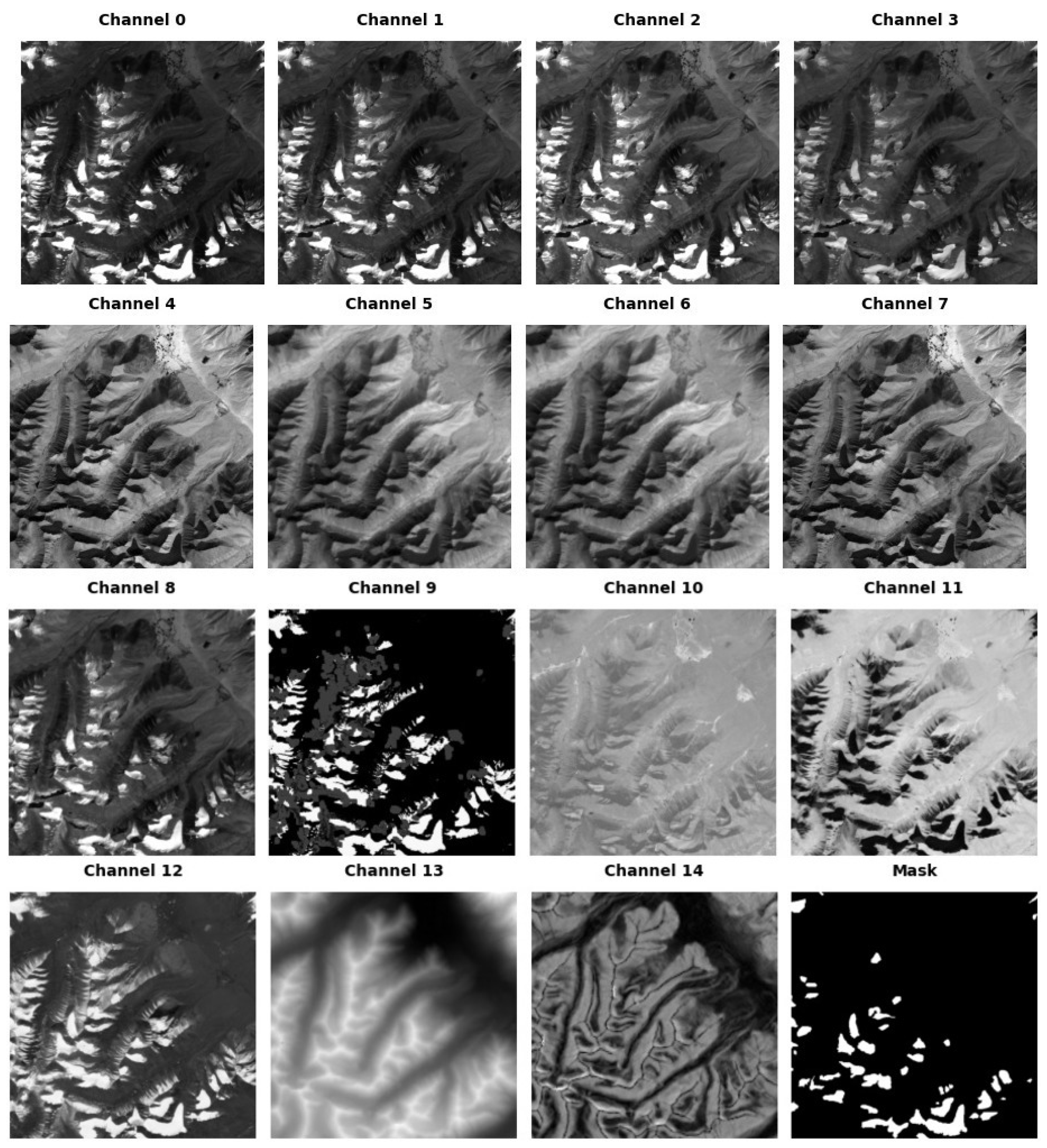
Figure 4.
Block diagram of the proposed segmentation scheme.
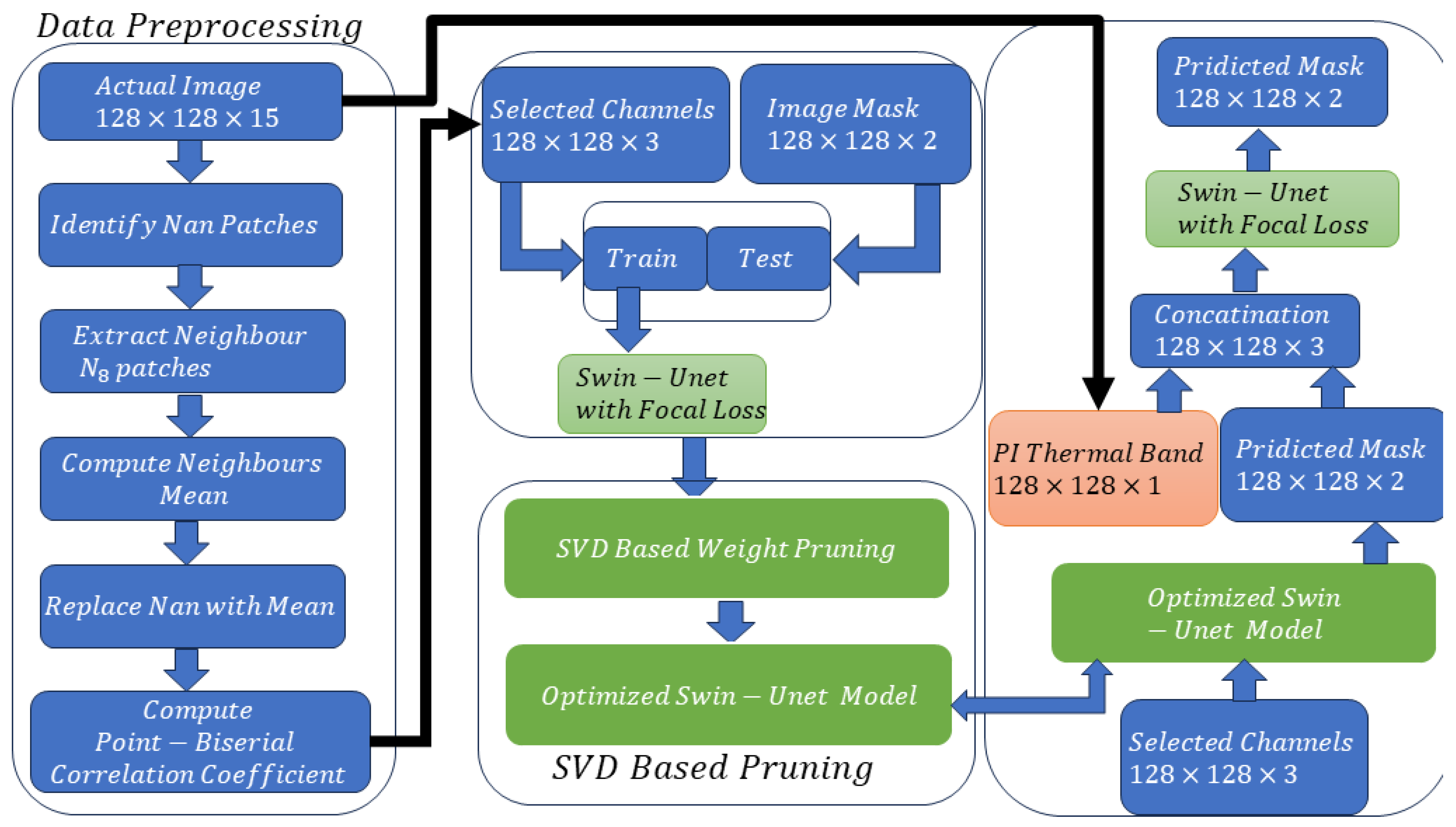
Figure 5.
Point-Biserial Correlation Matrix.
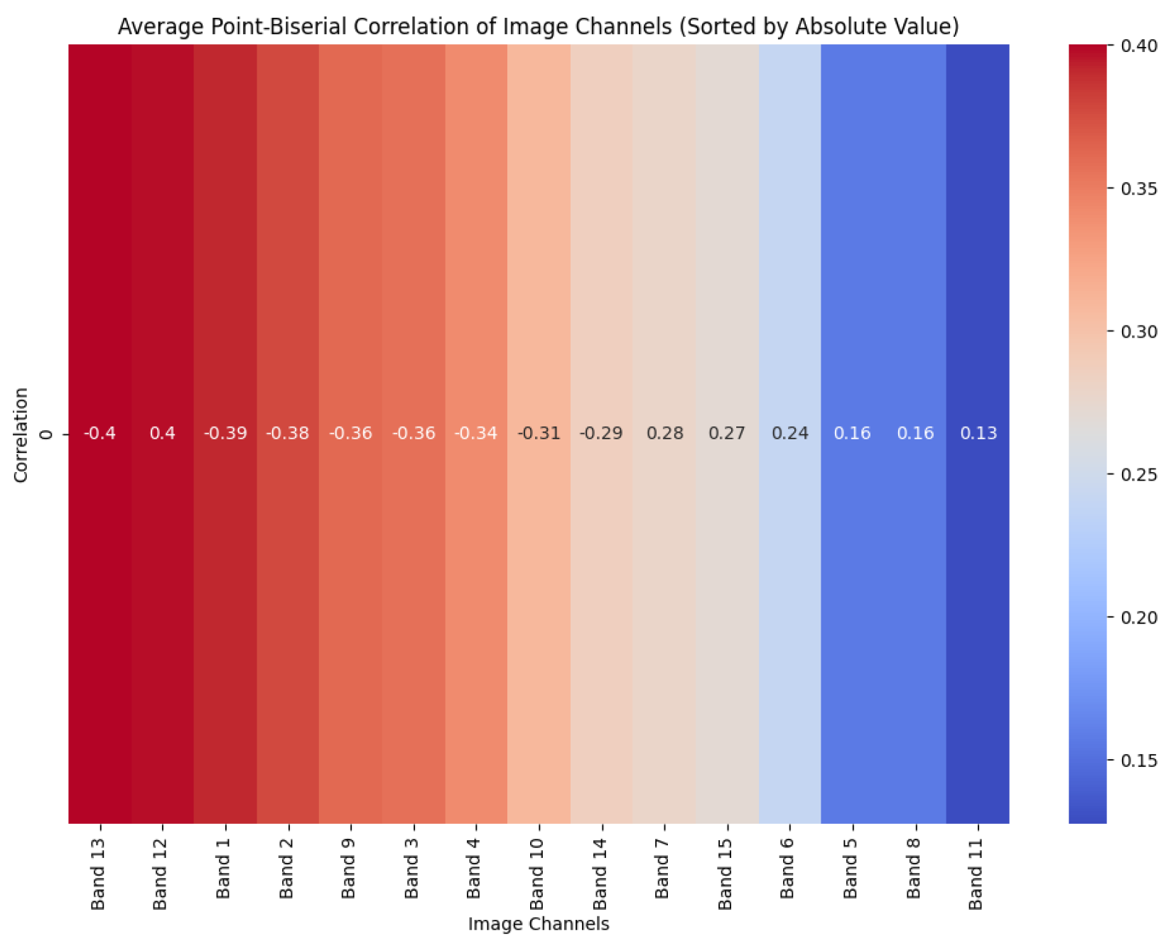
Figure 6.
Overview of the SPSW-UNet(SPSW-UNet) results. Each row, from top to bottom, showcases the input image, the original mask, the prediction by SPSW-UNet and the analysis of correct classifications.
Figure 6.
Overview of the SPSW-UNet(SPSW-UNet) results. Each row, from top to bottom, showcases the input image, the original mask, the prediction by SPSW-UNet and the analysis of correct classifications.
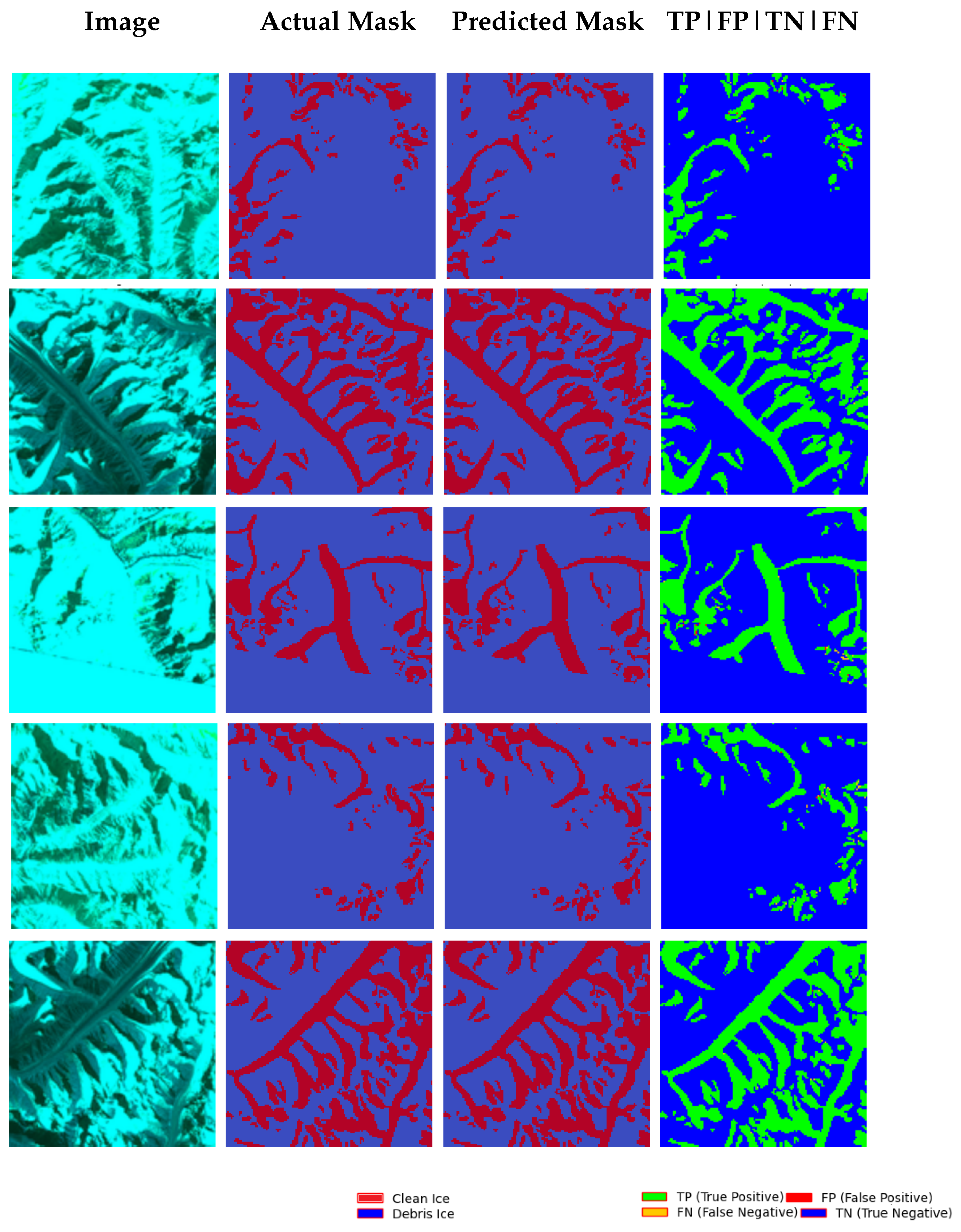
Table 2.
Comparative Analysis of the Cascaded Model Performance.
| Model | Acc. | F1 | Pre. | Rec. | IoU | AUC | IT (s) |
|---|---|---|---|---|---|---|---|
| Swin-UNet | 94.12% | 93.65% | 93.09% | 94.21% | 86.73% | 93.93% | 0.1865 |
| SPSW-UNet | 92.34% | 93.35% | 92.92% | 93.80% | 84.89% | 91.20% | 0.1247 |
| UNet-ResNet34 | 89.9% | 92.05% | 92.2% | 91.91% | 81.24% | 87.6% | 0.3059 |
| PICSw-UNet | 95.67% | 95.37% | 94.23% | 96.53% | 91.65% | 96.4% | 0.2795 |
Disclaimer/Publisher’s Note: The statements, opinions and data contained in all publications are solely those of the individual author(s) and contributor(s) and not of MDPI and/or the editor(s). MDPI and/or the editor(s) disclaim responsibility for any injury to people or property resulting from any ideas, methods, instructions or products referred to in the content. |
© 2025 by the authors. Licensee MDPI, Basel, Switzerland. This article is an open access article distributed under the terms and conditions of the Creative Commons Attribution (CC BY) license (http://creativecommons.org/licenses/by/4.0/).
Copyright: This open access article is published under a Creative Commons CC BY 4.0 license, which permit the free download, distribution, and reuse, provided that the author and preprint are cited in any reuse.


