
Submitted:
25 May 2025
Posted:
26 May 2025
You are already at the latest version
Abstract
In modern information systems, data analysis is pivotal for uncovering hidden patterns and extracting meaningful insights. Visualizing the behavior of real-valued functions over high-dimensional domains enables researchers to gain intuitive understanding of complex systems. Traditionally, mathematical problems are tackled analytically; however, a data-driven approach—where synthetic samples are explored systematically—can reveal new directions and solution spaces. In this paper, we introduce the RDSF algorithm, short for \textit{Reducing the Dimension of the Space of Independent and Dependent Variables of Real-Valued Functions}. This algorithm leverages manifold learning, specifically Multidimensional Scaling (MDS), to reduce the dimensionality of both input and output spaces, allowing effective visualization and analysis of function behaviors. We present a unified framework for analytical and visual exploration of mathematical and engineering problems using RDSF. The utility of RDSF is demonstrated through multiple case studies, including approximate solutions to partial differential equations (PDEs) and topological analysis of the distribution of prime numbers. These applications reveal that even abstract mathematical domains can benefit significantly from visual, data-oriented perspectives. The proposed framework is general, adaptable, and opens new avenues for exploration across disciplines.
Keywords:
RDSF algorithm
; manifold learning
; dimensionality reduction
; data-driven mathematics
; partial differential equations
; prime number topology
; scientific visualization
1. Introduction
Visual exploration of high-dimensional datasets often reveals subtle patterns, structural anomalies, or deviations from expected objective function behaviors. These insights can uncover new solution pathways or isolate subspaces of particular interest within the data landscape [1].
Manifold learning, situated at the intersection of geometry, computation, and statistics, has become a pivotal framework in modern data analysis [2]. It aims to uncover low-dimensional structures embedded within high-dimensional spaces [3]. Classic linear techniques such as Principal Component Analysis (PCA) [4]) and Multidimensional Scaling (MDS) [5]) provide interpretable projections by preserving variance or pairwise distances, respectively.
Understanding the behavior of functions involving more than three variables remains a critical challenge. Visualizing such high-dimensional relationships enhances the interpretability of model dynamics and variable interactions [6].
In this article, we introduce the Reducing the Dimension of the Space of Independent and Dependent Variables of Real-Valued Functions (RDSF), a novel computational algorithm that builds on MDS for dimensionality reduction and leverages random sampling to approximate objective landscapes. RDSF is particularly well-suited for cases where analytical formulations are unavailable or incomplete but a computable objective function exists.
We demonstrate the power and versatility of RDSF through three representative applications: (1) the approximation of solutions to partial differential equations (PDEs), (2) analysis of the distribution of prime numbers in multi-dimensional lattices, and (3) topological characterization of function behaviors. In each case, RDSF serves as a tool for converting computationally intractable problems into visually and numerically analyzable forms [7,8].
2. Algorithm for Reducing the Dimension of the Space of Independent and Dependent Variables of Real-Valued Functions (RDSF)
Let be an information space with dimension n, and let be a real-valued function defined over M. The goal of the RDSF algorithm is to analyze and visualize the behavior of f across M by constructing an interpretable geometric representation in , where the third dimension corresponds to the functional value of f at each point.
To achieve this, we employ **Multidimensional Scaling (MDS)**, a manifold learning technique that projects high-dimensional data into lower dimensions while preserving pairwise distances as closely as possible [9]. Preserving these distances ensures that the relative geometric and topological relationships among points in M are reflected in the reduced space.
The algorithm consists of the following steps:
- For each point , compute the function value .
- Apply MDS to the point cloud in M to obtain a 2D embedding in a new space , such that the Euclidean distances are preserved:
- For each embedded point , associate the corresponding function value , forming a new 3D representation:
- Visualize the set in . This 3D embedding enables intuitive analysis of the functional landscape, highlighting patterns such as gradients, clusters, local extrema, and other structural insights into the original function f.
This method is particularly useful for exploring the behavior of high-dimensional functions in optimization, approximation, and data analysis, especially where interpretability and visualization are important.
3. Applications of the RDSF Algorithm
The RDSF algorithm provides a powerful computational framework for analyzing a wide variety of mathematical and engineering problems. In many real-world scenarios, sufficient data can be collected or derived to construct an informative feature space. This allows for systematic evaluation of an objective function over varying parameters, forming what we call the M-space.
For theoretical problems, however, such data may not be readily available or might need to be generated synthetically. In such cases, the RDSF algorithm leverages random sampling and repeated simulations to iteratively refine the understanding of the objective landscape. This ability to explore solution spaces with minimal initial assumptions makes RDSF particularly valuable for high-dimensional, underdetermined, or nonlinear problems.
In the following subsection, we demonstrate the utility of the RDSF algorithm in approximating solutions to Partial Differential Equations (PDEs), a fundamental class of problems in mathematics and applied sciences.
3.1. Solving Partial Differential Equations Using RDSF
Partial Differential Equations (PDEs) are ubiquitous in modeling physical systems, from heat transfer to fluid dynamics [10]. However, analytical solutions are often intractable, necessitating approximate and numerical methods [11]. Here, we introduce a theoretical result that justifies the use of RDSF in approximating solutions to a general class of PDEs using randomly generated functional forms.
Definition 1.
A real-valued function is called a Finitely and Analytically Differentiable Function (FADF) if the function and all its partial derivatives of any order exist and remain finite over the domain of interest.
Example 1.
The functions and are examples of FADF functions.
Theorem 1.
Let be a PDE with finite coefficients over the domain of its independent variables . Then there exists a FADF function and a small constant such that the function
approximately satisfies the equation , where is a known continuous function and k represents the degree of the equation.
Proof.
The detailed proof constructs an approximate solution by inserting a perturbed FADF-based function into the PDE. Due to the boundedness of derivatives and the finiteness of coefficients, the residual can be bounded above and made arbitrarily small by choosing an appropriate . For brevity, we refer the reader to the appendix for a full derivation. □
Corollary 1.
In practice, due to the complexity of high-dimensional PDEs, the exact value of ε is unknown. The RDSF algorithm enables us to estimate a near-optimal value of ε through random sampling and numerical evaluation of the residual over many realizations of X.
Example 2
(Heat Equation in Four Variables). Consider the heat equation:
Let the trial solution be:
with initial choice .
Using the RDSF algorithm, we generate 500 random samples of in a bounded domain and compute . The residuals are visualized in Figure 1.
To improve accuracy, we repeat this process for and (Figure 2, Figure 3). The dispersion reduces as ε decreases.
From these results, we determine that the function
is a highly accurate approximate solution to the given PDE under the examined conditions.
3.2. Analysis and Investigation of the Dispersion of Prime Numbers
The distribution of prime numbers has long been a central theme in number theory and remains one of the most intriguing subjects in mathematics [12,13]. In this section, we demonstrate how the RDSF algorithm can be applied to analyze the dispersion pattern of prime numbers from a topological perspective, using synthetic integer spaces.
We construct an n-dimensional grid M, where each coordinate can take an integer value from 1 to 9. Each point represents a vector , and the product defines a non-prime candidate. We define the objective function as follows:
This function measures the “distance” from each constructed number to the next prime [14]. We apply the RDSF algorithm to build the corresponding topological spaces and visualize the distribution of across the grid. The results for 2D, 3D, 4D, and 5D spaces are combined in a unified visualization shown in Figure 4.
In the two-dimensional case, the values of range from 1 to 5 with frequencies of 14, 9, 5, 4, and 4, respectively. The highest concentration occurs at and , indicating that most products lie very close to a prime number.
In the three-dimensional case, spans a broader range: 1 through 13. The most frequent values are again within the range 1 to 5, with frequencies of 37, 18, 11, 9, and 13. A few outlier values like 11 and 13 appear with low frequency, illustrating the increased variability of prime gaps in higher dimensions.
In the four-dimensional case, takes values between 1 and 20. Notably, the frequency remains concentrated within to , with the highest at (75 instances). A few new values like emerge as dimensionality increases.
In the five-dimensional case, the dispersion of extends further, ranging from 1 to 31. Despite this, the values of are still highly concentrated in the range 1 to 13. Outliers such as and 31 occur with very low frequency. These results suggest that as the dimensionality increases, while more variation in the distance to the next prime emerges, the likelihood of small prime gaps remains dominant [15].
Based on the empirical distribution of observed in multiple dimensions, we propose the following corollary:
Corollary 2.
Let and define . Then, the probability that is a prime number decreases as t increases, and is maximized when .
This result indicates that within bounded integer grids, products of small integers tend to be closely followed by prime numbers, and this proximity exhibits a structured pattern across dimensions. The RDSF algorithm thus reveals an underlying topological signature in the dispersion of prime numbers.
3.3. Analysis and Investigation of the Behavior of Multivariate Arbitrary Real-Valued Functions
Let be a real-valued function of n variables. The RDSF algorithm provides a novel geometric and topological perspective for analyzing the behavior of such functions in a neighborhood of interest. Using Python, we randomly generate points from a specified domain to construct the M-space, where each point corresponds to an input vector of the function. The greater the number of points sampled, the more accurate the resulting analysis becomes.
Following the RDSF steps, we evaluate f at each sampled point and then use the MDS algorithm to reduce the n-dimensional input space into two dimensions while preserving pairwise distances. By incorporating the value of the function as the third coordinate, a 3D plot is obtained that reveals how the function behaves near the chosen region of the domain.
Example 3.
Rastrigin Function. This is a widely-used benchmark in multivariate optimization. Its highly multimodal structure makes it a difficult problem for optimization algorithms [16]:
where:
- is an n-dimensional input vector,
- A is a constant (typically set to 10),
- n is the number of variables.
In the two-variable case, the function surface contains numerous local minima (see Figure 5). Applying the RDSF algorithm reveals this complex landscape.
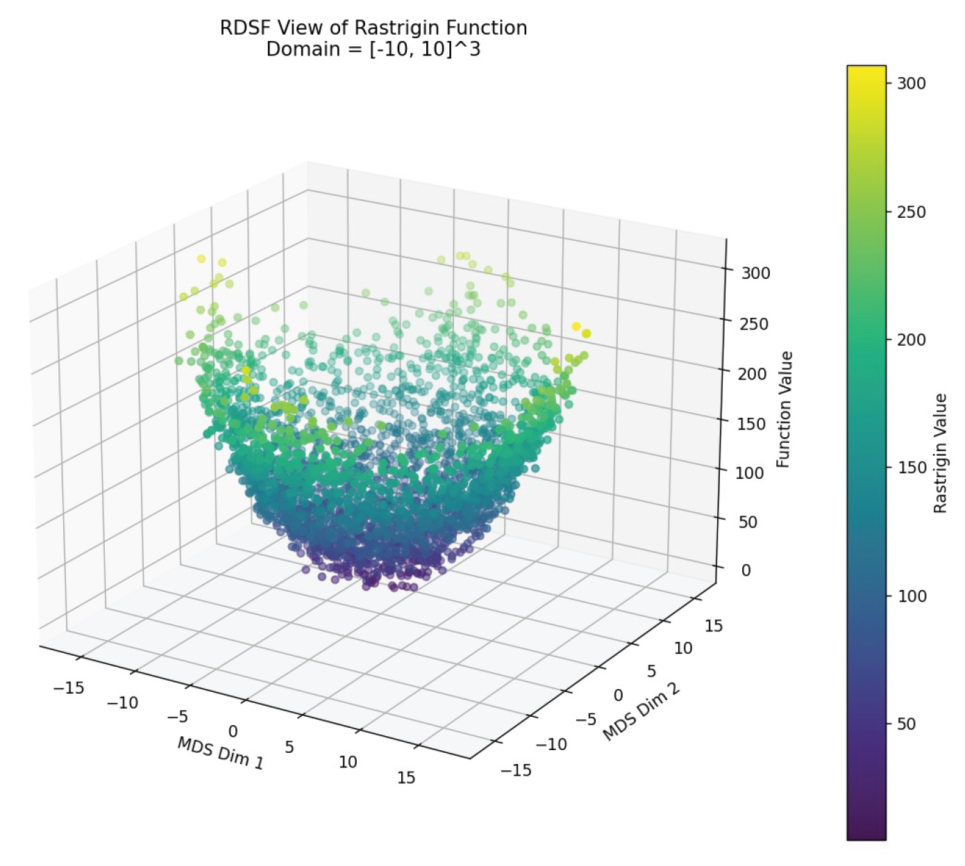
For three variables, where direct 4D visualization is impossible, traditional analysis often requires fixing one variable. In contrast, RDSF embeds the entire 3D space into 2D and then adds the function value to visualize a 3D structure (see Figs. Figure 6 and Figure 7).
In both ranges, the RDSF algorithm successfully reveals the dense distribution of local minima and the global minimum at the origin, consistent with known analytical results [16].
Example 4.
Ackley Function. Another benchmark in multivariate optimization, characterized by a nearly flat outer region and a central hole with a global minimum [17]. Its complexity, featuring numerous local minima, poses a significant challenge. The n-dimensional Ackley function is defined as:
where , and recommended parameters are , , . The global minimum occurs at , where .
1. Intuitive Visualization Using RDSF.We applied the RDSF algorithm to the 3-variable Ackley function without fixing any variable. Using Python, 300 random samples in were generated and evaluated. MDS was applied to embed into 2D, and the function values were used as the third coordinate.
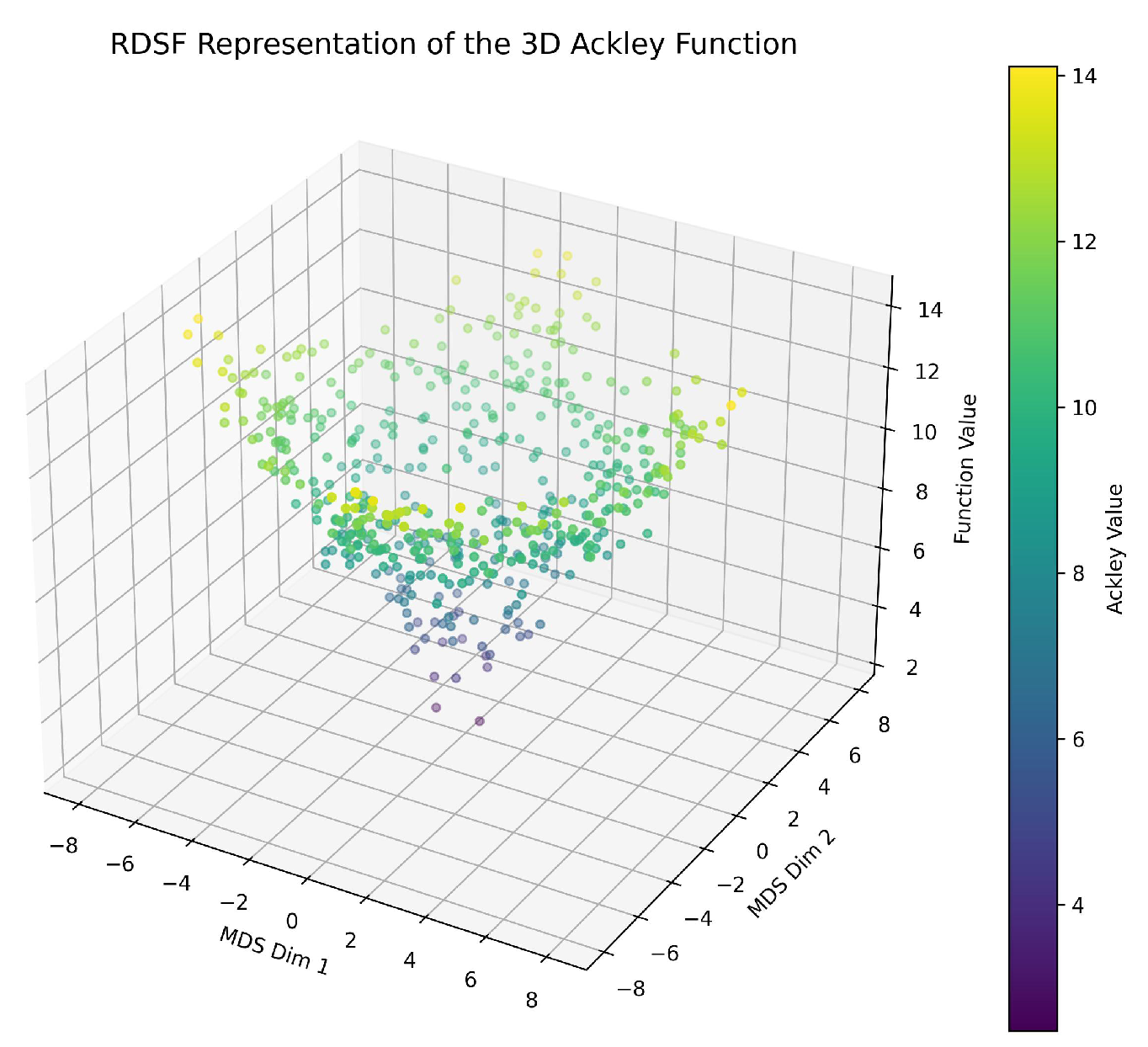
Figure 8.
Three-dimensional RDSF representation of the 3-variable Ackley function
As shown, RDSF reveals a central basin (global minimum) surrounded by ridges. This provides intuitive insight into how regions of similar output are arranged in input space.
2. Comparison with Numerical Optimization.To validate these insights, we used Particle Swarm Optimization (PSO) via thepyswarmslibrary [18,19]. With 40 particles and 100 iterations in , PSO found a near-global minimum:
- Estimated minimum:
- At point:
This aligns well with the RDSF visualization, supporting RDSF’s utility as both an exploratory and complementary tool for numerical optimization.
This section highlights the flexibility and insight provided by RDSF in exploring complex function behaviors, whether the functions are highly multimodal (like Rastrigin and Ackley) or smooth with a single minimum. The method enables a unified framework for analyzing arbitrary multivariate real-valued functions without requiring dimension-specific assumptions.
4. Conclusions
In this paper, we introduced the RDSF algorithm—Reducing the Dimension of the Space of Independent and Dependent Variables of Real-Valued Functions—a framework built upon manifold learning principles [20], specifically using MDS for dimensionality reduction [21]. RDSF enables visual exploration of high-dimensional function behavior by projecting independent variables into two dimensions and mapping function values as the third dimension.
We demonstrated its effectiveness across diverse problems: analyzing residuals in the heat equation [22] and revealing structural patterns in prime number distributions [23]. These case studies illustrated how RDSF provides a flexible tool for understanding the behavior of real-valued functions in multidimensional domains.
The visual representations produced by RDSF not only support exploratory data analysis [21] but also offer intuitive insights into mathematical and computational problems. We believe this framework can be extended to other analytical domains, enabling new methods of visualization and interpretation for complex systems.
Appendix A. Proof of Theorem 1
We provide a justification for the theorem stating that for a PDE with finite coefficients, there exists an approximate solution of the form
where is a FADF function, is a known continuous function, k represents the degree of the equation, and is a small constant.
Step 1: Structure of the PDE
Assume the PDE is composed of partial derivatives of U with respect to variables and possibly nonlinear combinations of these derivatives. Let us denote the PDE in general form:
where: - is a multi-index of derivative orders, - denotes the partial derivative of order , - are finite-valued coefficient functions, - is a smooth nonlinear expression in U and its derivatives.
Step 2: Inserting the Trial Function
Let , with f being FADF and G continuous. Then all required derivatives of U exist and are finite:
Step 3: Plug into the PDE
We substitute into :
This simplifies to:
Note that: - The first term is because is factored out. - The second term, , can be expanded in a Taylor series around :
for some bounded function depending on the partials of f and G.
Step 4: Estimating the Residual
Combining both terms:
for some bounded function . Hence, the total residual is:
Appendix Step 5: Conclusion
Therefore, by choosing small enough, we can ensure that the residual becomes arbitrarily small across the domain of interest. This justifies that is an approximate solution to the PDE:
References
- Keim, D. A., Mansmann, F., Schneidewind, J., Thomas, J., & Ziegler, H. (2008). Visual analytics: Scope and challenges. In Visual Data Mining, pp. 76–90. Springer.
- Ma, Y.; Fu, Y. Manifold Learning Theory and Applications; CRC Press, 2011. [Google Scholar]
- Lee, J. A.; Verleysen, M. Nonlinear Dimensionality Reduction; Springer, 2007. [Google Scholar]
- Jolliffe, I. T. Principal Component Analysis; Springer Series in Statistics; 2002. [Google Scholar]
- Borg, I.; Groenen, P. J. F. Modern Multidimensional Scaling: Theory and Applications; Springer, 2005. [Google Scholar]
- Buja, A.; Cook, D.; Swayne, D. F. Interactive high-dimensional data visualization. Journal of Computational and Graphical Statistics 2008, 17(4), 880–900. [Google Scholar] [CrossRef]
- Raissi, M.; Perdikaris, P.; Karniadakis, G. E. Physics-informed neural networks: A deep learning framework for solving forward and inverse problems involving nonlinear partial differential equations. Journal of Computational Physics 2019, 378, 686–707. [Google Scholar] [CrossRef]
- Sarnak, P. Some Applications of Modular Forms. In Cambridge Tracts in Mathematics; Cambridge University Press, 1989; Vol. 99. [Google Scholar]
- Kruskal, J. B.; Wish, M. Multidimensional Scaling; Sage Publications, 1978. [Google Scholar]
- Evans, L. C. Partial Differential Equations; American Mathematical Society, 2010. [Google Scholar]
- Quarteroni, A.; Sacco, R.; Saleri, F. Numerical Mathematics. Springer Science & Business Media, 2007. [Google Scholar]
- Hardy, G. H.; Wright, E. M. An Introduction to the Theory of Numbers, 6th edition; Oxford University Press, 2008. [Google Scholar]
- Ribenboim, P. In The Little Book of Bigger Primes; Springer-Verlag, 1996.
- Granville, A. Harald Cramér and the distribution of prime numbers. Scandinavian Actuarial Journal 1995, 1, 12–28. [Google Scholar] [CrossRef]
- Pintz, J. Cramér vs. Cramér: On Cramér’s probabilistic model for primes. Functiones et Approximatio 2007, 37(2), 361–376. [Google Scholar] [CrossRef]
- Rastrigin, L. A. (1974). Systems of extremal control. Mir, Moscow.
- Ackley, D. H. A Connectionist Machine for Genetic Hillclimbing; Kluwer Academic Publishers, 1987. [Google Scholar]
- Kennedy, J.; Eberhart, R. Particle swarm optimization. In Proceedings of ICNN’95 - International Conference on Neural Networks; IEEE, 1995. [Google Scholar]
- Miranda, L. pyswarms: a research toolkit for particle swarm optimization in Python. Journal of Open Source Software 2020, 5(50), 1996. [Google Scholar]
- Ma, Y.; Fu, Y. Manifold Learning Theory and Applications; CRC Press, 2011. [Google Scholar]
- Borg, I.; Groenen, P. J. F. Modern Multidimensional Scaling: Theory and Applications; Springer Science & Business Media, 2005. [Google Scholar]
- Strauss, W. A. Partial Differential Equations: An Introduction; John Wiley & Sons, 1992. [Google Scholar]
- Apostol, T. M. Introduction to Analytic Number Theory; Springer, 1976. [Google Scholar]
- Tenenbaum, J. B.; de Silva, V.; Langford, J. C. A global geometric framework for nonlinear dimensionality reduction. Science 2000, 290(5500), 2319–2323. [Google Scholar] [CrossRef] [PubMed]
- McInnes, L.; Healy, J.; Melville, J. UMAP: Uniform Manifold Approximation and Projection for Dimension Reduction. arXiv preprint 2018, arXiv:1802.03426. [Google Scholar]
Figure 1.
Residuals for .
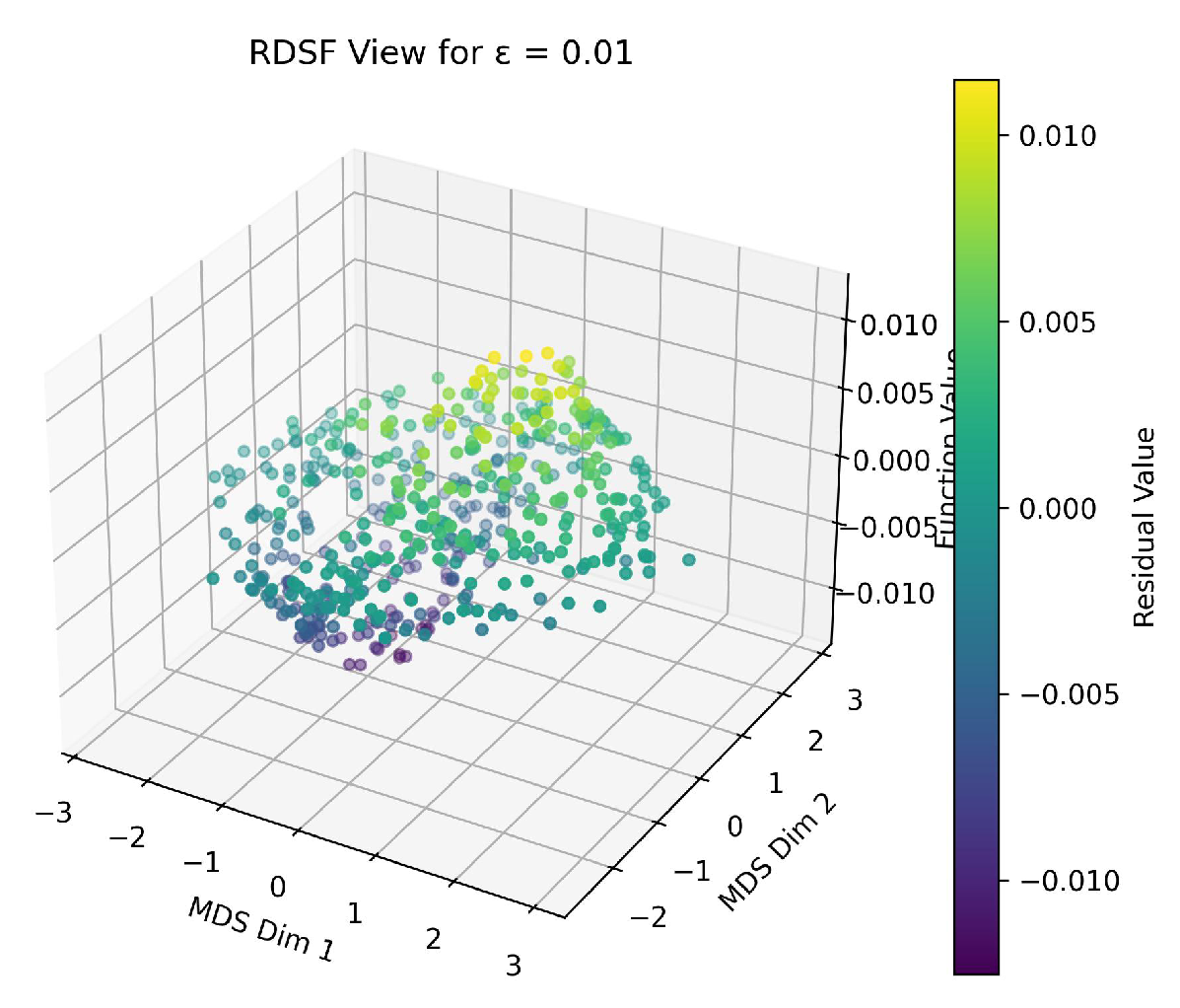
Figure 2.
Residuals for .
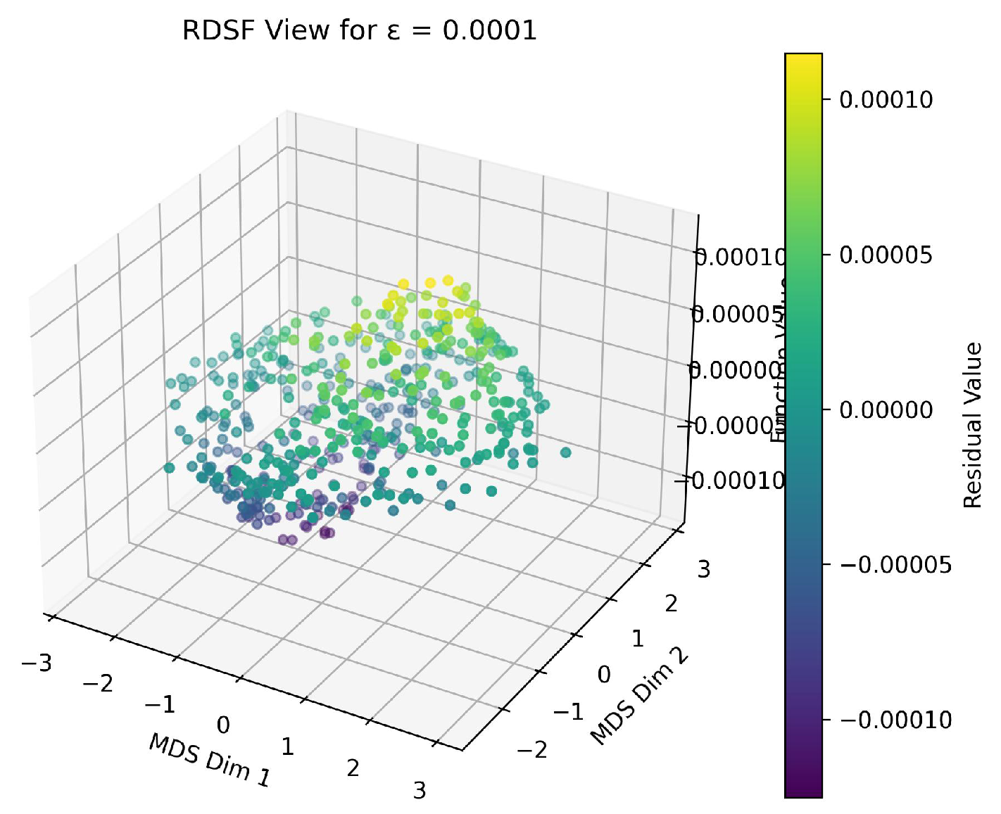
Figure 3.
Residuals for .
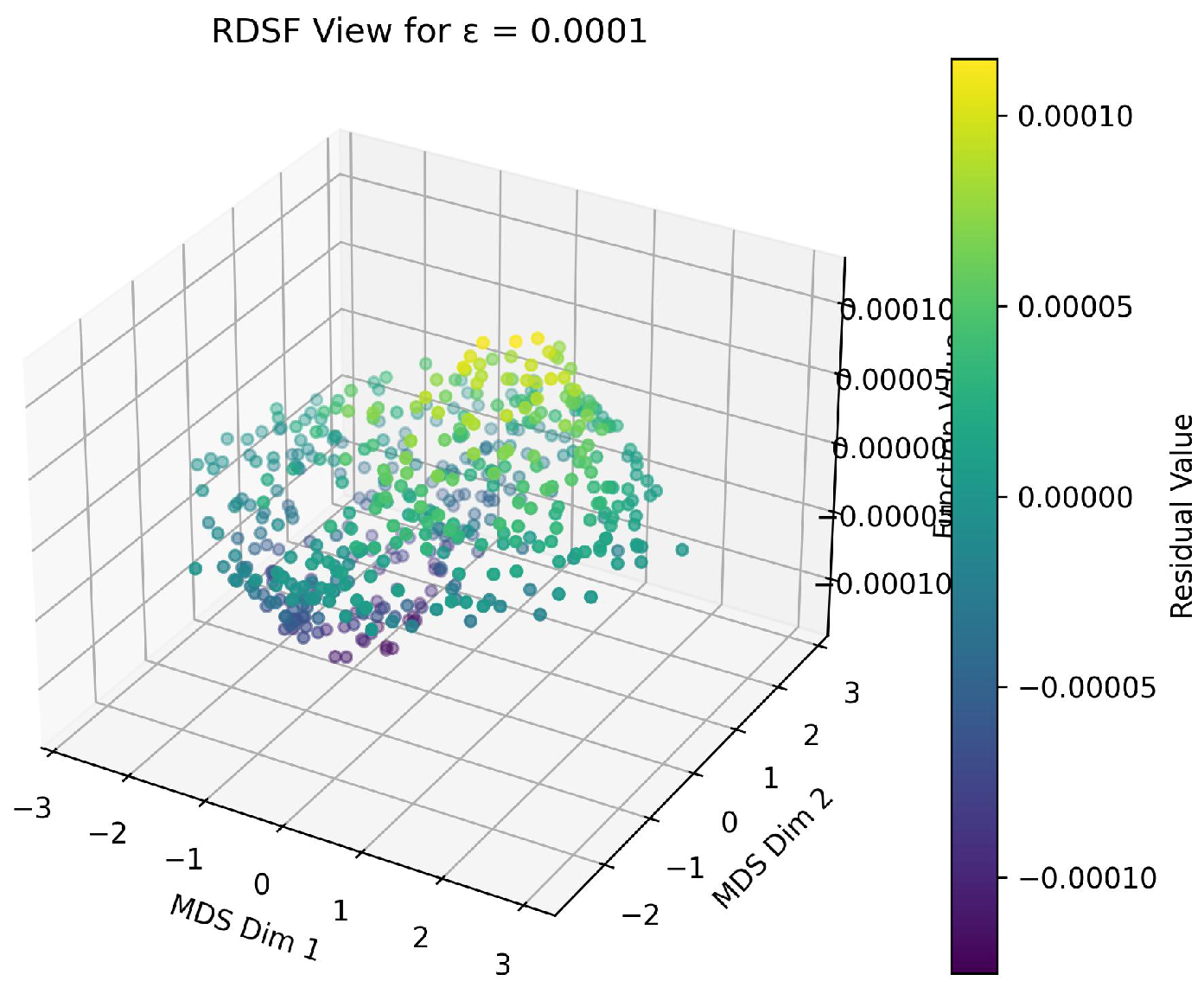
Figure 4.
Distribution of in 2D to 5D spaces: visualizing the distance to the next prime for synthetic integer vectors under the RDSF framework. Each subplot corresponds to a specific dimensionality (2D, 3D, 4D, 5D) and reveals the structured variation in the dispersion of prime distances across dimensions.
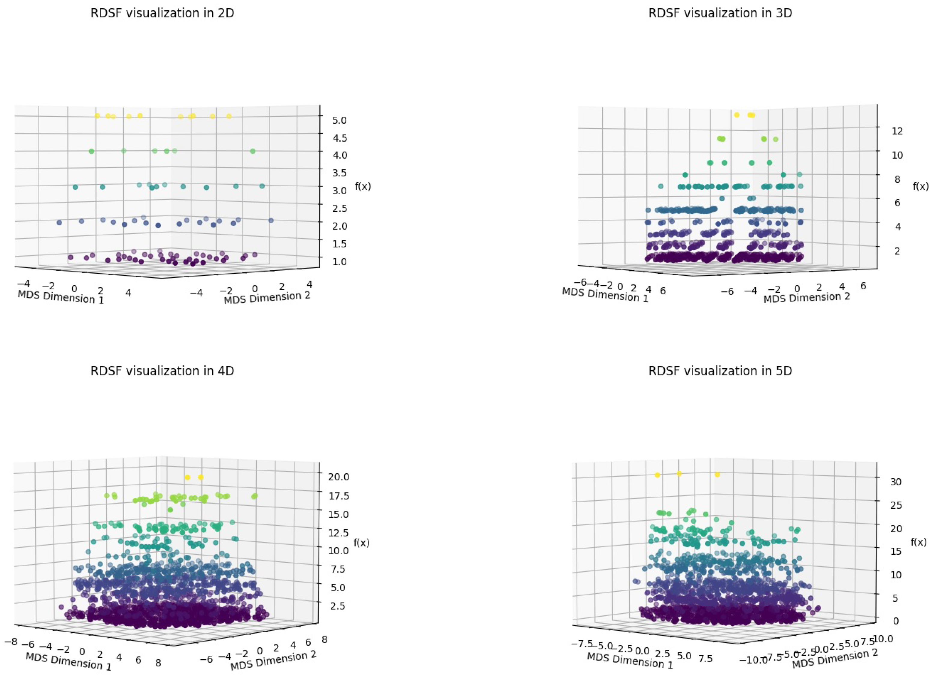
Figure 5.
Rastrigin Function (2 variables) in the range
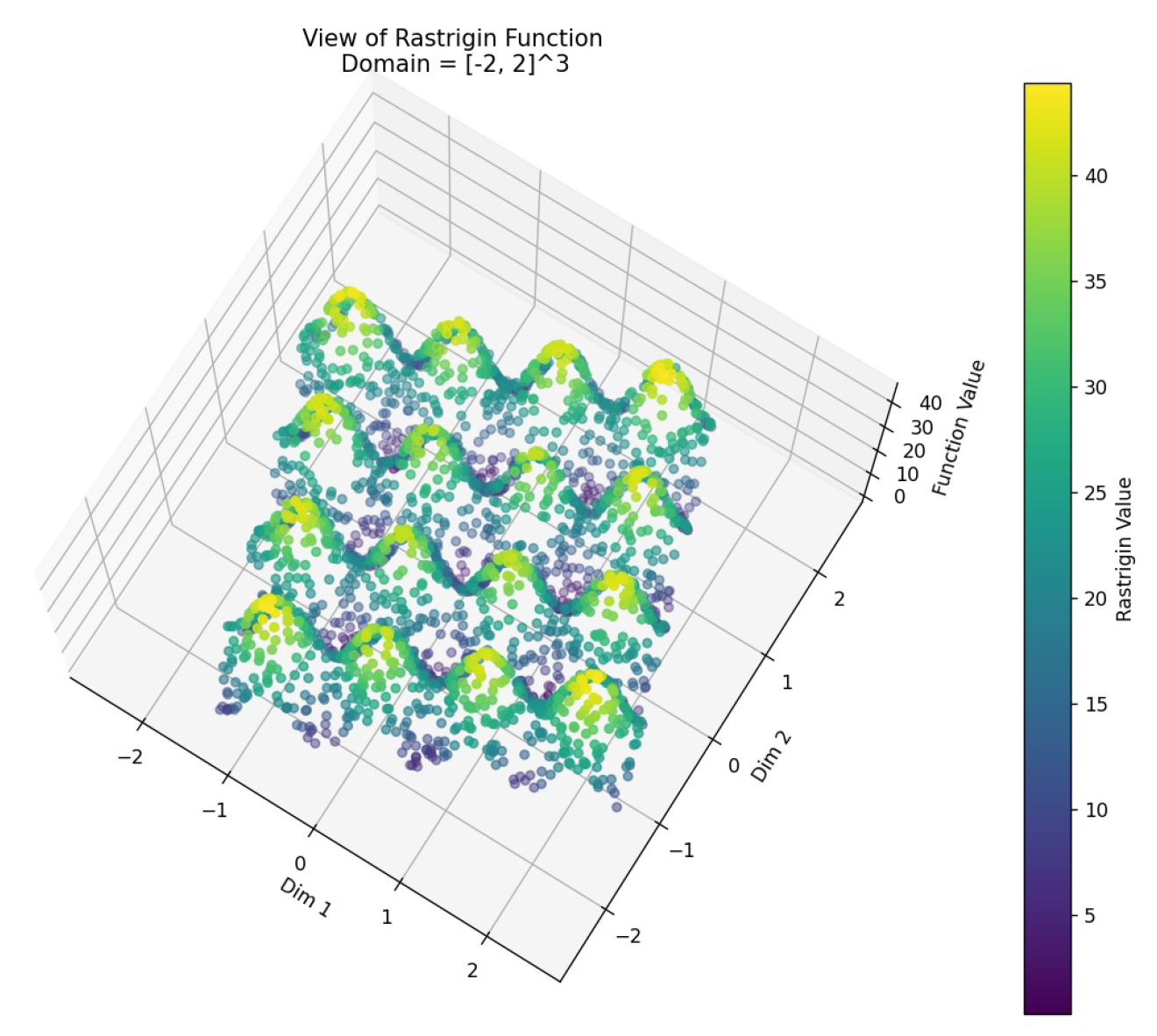
Figure 6.
Rastrigin Function (3 variables) in the range
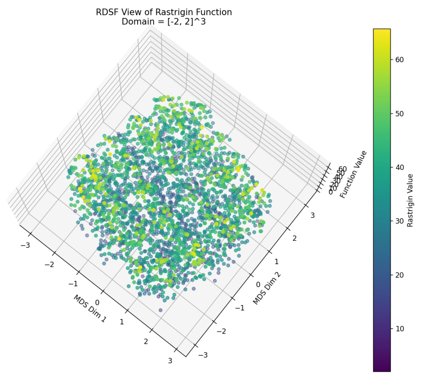
Figure 7.
Rastrigin Function (3 variables) in the range
Disclaimer/Publisher’s Note: The statements, opinions and data contained in all publications are solely those of the individual author(s) and contributor(s) and not of MDPI and/or the editor(s). MDPI and/or the editor(s) disclaim responsibility for any injury to people or property resulting from any ideas, methods, instructions or products referred to in the content. |
© 2025 by the authors. Licensee MDPI, Basel, Switzerland. This article is an open access article distributed under the terms and conditions of the Creative Commons Attribution (CC BY) license (http://creativecommons.org/licenses/by/4.0/).
Copyright: This open access article is published under a Creative Commons CC BY 4.0 license, which permit the free download, distribution, and reuse, provided that the author and preprint are cited in any reuse.


