Bridging Smoothness and Fractality: A Banach Space Framework for Hybrid Regularity with Spectral and Geometric Applications

1. Introduction

Recent advances in the analysis of complex systems have revealed the need to develop function spaces that can simultaneously capture smooth and fractal behaviors. Classical Sobolev spaces $W^{s,2}(\Omega )$ adequately model smooth phenomena, yet they fail to account for local irregularities present in many real-world signals and images. On the other hand, purely fractal or Besov-type spaces can capture these irregularities but often lack the global stability required for numerical and spectral methods.

In this work, we introduce the hybrid space

$$B^{s,\alpha }(\Omega )=W^{s,2}(\Omega )\cap F^{\alpha }(\Omega ),$$

which unifies the two paradigms. Our contributions include:

• The establishment of the Banach space property and continuous Hölder embedding for $B^{s,\alpha }(\Omega )$.
• A detailed spectral analysis of truncated self-adjoint operators acting on $B^{s,\alpha }(\Omega )$.
• Robust estimates for the local Hausdorff dimension of function graphs, including a measurable partition of the domain into smooth and fractal regions.
• A thorough literature review (sec:stateart) encompassing 39 key references, which validates and contextualizes our approach.

The remainder of the paper is organized as follows. Section 2 details the state of the art, reviewing relevant literature. Section 3 introduces basic notations and definitions. Section 4 is devoted to the construction and mathematical properties of the hybrid space. Section 5 and Section 6 treat, respectivelly, the spectral analysis and the local geometrical properties. Section 7 investigates robustness under perturbations. Numerical illustrations and potential applications are presented in Section 8. We conclude in Section 10 with a discussion and perspectives on future work.

2. State of the Art

The study of functional spaces with mixed regularity has emerged as a central topic in modern mathematical analysis, motivated by the need to model complex systems that exhibit both smooth and highly irregular features. Classical Sobolev spaces $W^{s,2}(\Omega )$, introduced by Sobolev [1] and extended by Triebel [2,3], provide a robust framework for characterizing smoothness via integrability of derivatives. In parallel, fractal analysis, shaped by Mandelbrot’s pioneering work [4,5] and formalized through Hausdorff measures [6], has proven essential in describing irregular and self-similar structures arising in natural and artificial systems.

However, many real-world signals—such as turbulent flows [7], financial time series [5], or biomedical images [8]—exhibit **hybrid regularity**, where neither classical smoothness nor pure fractality is sufficient to describe the underlying geometry. This has led to a growing interest in **unified frameworks** capable of accommodating both behaviors.

Early attempts to bridge this divide include **Besov spaces**, which generalize Sobolev spaces by integrating Hölder-type control and capturing more nuanced local behavior [2,9]. Wavelet-based decompositions have refined their practical usability [10,11,12], with significant impact in signal and image processing. However, Besov spaces often assume a **uniform regularity** across the domain, limiting their expressiveness for sharply transitioning or multiscale structures.

In response, **fractional Sobolev spaces** were introduced [13,14] to extend embedding capabilities. These spaces offer smoother interpolation between classical function spaces but lack explicit control over **geometric fractality**. Consequently, they are not optimal for characterizing singularities or local dimension variations, which are crucial in applications such as porous media or multifractal turbulence.

On the **spectral side**, foundational work by Kato [15] and later by Engel and Nagel [16] laid the theoretical groundwork for perturbation and stability theory of linear operators. These ideas were extended to more general settings by Davies [17] and adapted to fractal domains by Strichartz [18,19] and Kigami [20]. More recent developments have focused on **spectral properties in hybrid spaces**. For instance, Cheeger and Kleiner [21] explored metric measure spaces with mixed geometric properties, and Alberti et al. [22] introduced analytical tools for fractal currents. Spectral stability in the context of chaotic systems was notably advanced by Borthwick [23] and Dyatlov and Zworski [24].

In parallel, **numerical methods** adapted to hybrid geometries have matured significantly. Arneodo et al. [25] and Jacques et al. [26] developed wavelet-based tools tailored to local scaling laws. Compressed sensing and sparse approximation strategies—pioneered by Donoho [27] and Candès et al. [28]—have proven powerful in representing signals exhibiting nonuniform smoothness. Adaptive spectral schemes [29,30] offer efficient solvers, though their extension to fractal-Sobolev hybrid spaces remains relatively unexplored.

Geometric approaches have also played a key role in understanding hybrid regularity. Gromov’s work on tangent structures in singular spaces [31] and Winter’s recent study of fractal manifolds [32] illustrate the deep geometric underpinnings of mixed regularity. In dynamics, Baladi [33] and Liverani [34] explored interrupted linearity and its implications for stability, with consequences in areas such as **quantum chaos** [35].

In this article, we introduce the hybrid function space $B^{s,\alpha }(\Omega )=W^{s,2}(\Omega )\cap F^{\alpha }(\Omega )$, aiming to **overcome the limitations** of previous frameworks. Unlike Besov spaces, $B^{s,\alpha }(\Omega )$ imposes explicit **geometric constraints** via a Besov-like norm. Compared to fractional Sobolev spaces, it allows **local dimension control** and fractal scaling. Our spectral results generalize Kato’s and Davies’ stability theorems [15,17] to operators on $B^{s,\alpha }(\Omega )$, while extending fractal spectral analysis initiated by Strichartz and Borthwick [19,23]. The **local dimension estimates** build on Frostman’s lemma [36] and Mattila’s refinements [37], and the **stability under perturbations** is aligned with the recent advances by Dyatlov and Zworski [24].

By integrating these theoretical and computational advances, our contribution offers a **versatile and rigorous framework** for analyzing phenomena that lie at the intersection of smooth analysis, geometric measure theory, and fractal geometry. We believe $B^{s,\alpha }(\Omega )$ provides both the analytical robustness and the geometric sensitivity necessary for a wide range of modern applications.

3. Preliminaries and Notations

This section introduces the main function spaces used throughout the paper, as well as the notational conventions adopted to ensure clarity and coherence.

3.1. Function Spaces and Basic Definitions

Let $\Omega \subset {\mathbb{R}}^d$ be a bounded open domain with smooth boundary (e.g., $C^{\infty }$ or Lipschitz, depending on the context). We use the following standard function spaces:

• Lebesgue Spaces: $L^p(\Omega )$ denotes the space of measurable functions $f:\Omega \to \mathbb{R}$ such that ${\parallel f\parallel }_{L^p(\Omega )}<\infty$, where

  $${\parallel f\parallel }_{L^p(\Omega )}:={\left({\int }_{\Omega }{\left|f\left(x\right)\right|}^{p}dx\right)}^{1/p},1\le p<\infty .$$
• Sobolev Spaces: $W^{s,2}(\Omega )$ (also denoted $H^s(\Omega )$) refers to the fractional Sobolev space of order $s\ge 0$, defined via Fourier transform or interpolation, and consisting of functions with square-integrable derivatives (in the weak sense) up to order s:

  $${\parallel f\parallel }_{W^{s,2}(\Omega )}:={\left(\sum _{\left|\alpha \right|\le \lfloor s\rfloor }{\parallel {\partial }^{\alpha }f\parallel }_{L^2(\Omega )}^2+{\int }_{\Omega }{\int }_{\Omega }{\displaystyle \frac{{|f\left(x\right)-f\left(y\right)|}^2}{{|x-y|}^{d+2s}}}dxdy\right)}^{1/2}.$$
• Fractal (Hölder-type) Spaces: $F^{\alpha }(\Omega )$ for $\alpha >{\displaystyle \frac{d}{2}}$ is a function space that captures fine-scale, possibly irregular behavior. It may be defined in terms of Hölder norms or Besov norms, depending on the analytic framework. In particular, a possible norm is

  $${\parallel f\parallel }_{F^{\alpha }(\Omega )}:=\underset{x\ne y\in \Omega }{sup}{\displaystyle \frac{\left|f\right(x)-f(y\left)\right|}{{|x-y|}^{\alpha }}},$$

  when f is Hölder continuous of exponent $\alpha$.
• Hybrid Space: We define the intersection space

  $$B^{s,\alpha }(\Omega ):=W^{s,2}(\Omega )\cap F^{\alpha }(\Omega ),$$

  equipped with the combined norm

  $${\parallel f\parallel }_{B^{s,\alpha }(\Omega )}:={\parallel f\parallel }_{W^{s,2}(\Omega )}+{\parallel f\parallel }_{F^{\alpha }(\Omega )}.$$
  This hybrid space is designed to capture both global smoothness (via Sobolev structure) and local irregularity or fractality (via the fractal space).

3.2. Notational Conventions

The following conventions are used throughout the paper:

• The dimension of the ambient Euclidean space is denoted $d\in \mathbb{N}$.
• $\Omega \subset {\mathbb{R}}^d$ is always a bounded open domain with smooth boundary.
• The notation $f\in X\cap Y$ means that f belongs to both spaces X and Y, with the norm ${\parallel f\parallel }_{X\cap Y}:={\parallel f\parallel }_X+{\parallel f\parallel }_Y$.
• Embeddings of function spaces are denoted by $X\hookrightarrow Y$, meaning X is continuously embedded in Y.
• Local Hölder continuity or regularity is denoted by $C^{0,\beta }$ for some exponent $\beta >0$.
• The symbol ${\Gamma }_f$ denotes the graph of a function f, i.e., ${\Gamma }_f:=\{(x,f\left(x\right)):x\in \Omega \}$.
• ${dim}_H(·)$ denotes the Hausdorff dimension.
• $\parallel ·\parallel$ without a subscript always denotes the norm in the current context, which will be clear from usage.

3.3. Summary Table of Symbols

To aid the reader, we provide below a table summarizing the key notations used throughout the paper:

Symbol	Meaning
$\Omega$	Bounded open domain in ${\mathbb{R}}^d$ with smooth boundary
d	Dimension of the ambient space
$L^p(\Omega )$	Lebesgue space of p-integrable functions
$W^{s,2}(\Omega )$, $W^{s,2}(\Omega )$	Sobolev space of order s with $L^2$ integrability
$F^{\alpha }(\Omega )$, $F^{\alpha }(\Omega )$	Fractal (Hölder-type) space with exponent $\alpha$
$B^{s,\alpha }(\Omega )$, $B^{s,\alpha }(\Omega )$	Hybrid space: intersection $W^{s,2}\cap F^{\alpha }$
${\Gamma }_f$	Graph of function f, i.e., $\left\{\right(x,f\left(x\right)):x\in \Omega \}$
${dim}_H(·)$	Hausdorff dimension of a set
$X\hookrightarrow Y$	Continuous embedding from X into Y
${\parallel ·\parallel }_X$	Norm in the space X

These notations are consistently used throughout all definitions, theorems, and proofs in the sequel.

4. Construction of the Hybrid Space ${\mathbf{B}}^{\mathbf{s},\mathbf{\alpha }}(\Omega )$

Building upon the function spaces introduced in sec:preliminaries, we now construct and analyze the hybrid space $B^{s,\alpha }(\Omega )$, which lies at the intersection of Sobolev regularity and fractal structure. This space is designed to capture multiscale phenomena that combine global smoothness with local irregularity—features that arise naturally in complex signals and geometries.

4.1. Definition and Motivation

The classical Sobolev space $W^{s,2}(\Omega )$ ensures a certain degree of smoothness in the $L^2$-based framework. However, it is insufficient to describe fine-scale structures that exhibit local singularities or oscillations. On the other hand, the fractal-type space $F^{\alpha }(\Omega )$ imposes conditions on the pointwise behavior of functions, offering a window into local irregularity and fine-grained geometric features.

To model situations where both types of regularity are simultaneously relevant, we define the **hybrid space**

$$B^{s,\alpha }(\Omega ):=W^{s,2}(\Omega )\cap F^{\alpha }(\Omega ).$$

This space is equipped with the natural norm

$${\parallel f\parallel }_{B^{s,\alpha }(\Omega )}:={\parallel f\parallel }_{W^{s,2}(\Omega )}+{\parallel f\parallel }_{F^{\alpha }(\Omega )},$$

which combines the global energy-based Sobolev norm with the local scaling-sensitive fractal norm.

Remark 1.

The choice of additive norm ensures that convergence in $B^{s,\alpha }(\Omega )$ implies convergence in both components, making the space suitable for theoretical analysis and numerical approximation. Alternative norms, such as the maximum of the two, may be considered but are less standard in functional analysis.

Example 1.

Let $f\in H^s(\Omega )$ be smooth on most of Ω, except on a compact set $K\subset \Omega$ where it behaves like a fractional Brownian path with Hölder exponent $\alpha <s$. Then $f\in B^{s,\alpha }(\Omega )$ for suitable $s>{\displaystyle \frac{d}{2}}$ and $\alpha >{\displaystyle \frac{d}{2}}$, but $f\notin H^s(\Omega )\cap C^{0,\alpha }(\Omega )$, showing the added flexibility of the hybrid formulation.

4.2. Basic Properties and Functional Structure

We now study the fundamental analytical structure of the hybrid space $B^{s,\alpha }(\Omega )$. In particular, we establish that it is a Banach space, and describe its embedding into spaces of uniformly continuous functions.

Theorem 1

(Banach Space Structure and Hölder Embedding). Let $\Omega \subset {\mathbb{R}}^d$ be a bounded domain with smooth boundary, and suppose $s\ge 0$, $\alpha >{\displaystyle \frac{d}{2}}$. Then:

(a) 

$B^{s,\alpha }(\Omega )=W^{s,2}(\Omega )\cap F^{\alpha }(\Omega )$, endowed with the norm

$${\parallel f\parallel }_{B^{s,\alpha }(\Omega )}={\parallel f\parallel }_{W^{s,2}(\Omega )}+{\parallel f\parallel }_{F^{\alpha }(\Omega )},$$

is a Banach space.

(b) 

If $s>{\displaystyle \frac{d}{2}}$, then $B^{s,\alpha }(\Omega )\hookrightarrow C^{0,\beta }(\Omega )$ continuously, with

$$\beta :=min\left\{s-{\displaystyle \frac{d}{2}},\alpha -{\displaystyle \frac{d}{2}}\right\}.$$

Proof. 

(a)

Completeness: Both $W^{s,2}(\Omega )$ and $F^{\alpha }(\Omega )$ are Banach spaces when equipped with their respective norms. Since their intersection is endowed with the sum norm, the space $B^{s,\alpha }(\Omega )$ is also complete.

(b)

Embedding: For $s>{\displaystyle \frac{d}{2}}$, the Sobolev–Morrey embedding theorem guarantees that

$$W^{s,2}(\Omega )\hookrightarrow C^{0,s-{\displaystyle \frac{d}{2}}}(\Omega ).$$

Simultaneously, by the definition of $F^{\alpha }(\Omega )$, we assume that

$$F^{\alpha }(\Omega )\hookrightarrow C^{0,\alpha -{\displaystyle \frac{d}{2}}}(\Omega ).$$

It follows that any function in $B^{s,\alpha }(\Omega )$ belongs to $C^{0,\beta }(\Omega )$, where

$$\beta :=min\left\{s-{\displaystyle \frac{d}{2}},\alpha -{\displaystyle \frac{d}{2}}\right\}.$$

This embedding is continuous since both constituent embeddings are.

□

Remark 2.

The condition $s>{\displaystyle \frac{d}{2}}$ is essential to ensure that functions in $W^{s,2}(\Omega )$ are continuous. This is sharp in general. Similarly, the assumption $\alpha >{\displaystyle \frac{d}{2}}$ ensures pointwise control for elements of $F^{\alpha }(\Omega )$, allowing their graph to be analyzed geometrically.

Remark 3

(Comparison with Besov Spaces). Besov spaces $B_{p,q}^s(\Omega )$ interpolate between Sobolev and Hölder spaces, and include control over both smoothness and scaling. However, they usually assume uniform regularity. In contrast, $B^{s,\alpha }(\Omega )$ allows one to explicitly combine smooth global behavior with localized fractal constraints, offering a more flexible modeling framework in heterogeneous domains.

Remark 4

(Duality and Extension). One may define a dual space ${\left(B^{s,\alpha }(\Omega )\right)}^{\prime }$, whose elements act on test functions belonging to $B^{s,\alpha }(\Omega )$. In practice, the characterization of the dual depends heavily on the definition of $F^{\alpha }(\Omega )$. In applications such as image analysis or PDEs on rough domains, this duality plays a role in defining weak formulations.

5. Spectral Analysis of Truncated Operators

In many analytical and numerical settings, especially when working within infinite-dimensional function spaces such as $B^{s,\alpha }(\Omega )$, one is often led to consider finite-dimensional approximations of linear operators. These approximations are not only necessary for computation, but they also offer theoretical insights into the behavior of spectra under restriction or discretization.

In this section, we study the **spectral stability** of such approximations in the hybrid space framework. More precisely, we analyze the behavior of the spectrum of an operator T when it is projected onto a finite-dimensional subspace of $B^{s,\alpha }(\Omega )$.

5.1. Truncation and Spectral Perturbation

Let $T:D\left(T\right)\subset B^{s,\alpha }(\Omega )\to B^{s,\alpha }(\Omega )$ be a **bounded, self-adjoint linear operator**, such as an elliptic differential operator, or an integral operator with symmetric kernel. In applications, we are often restricted to finite-dimensional subspaces $K\subset B^{s,\alpha }(\Omega )$, e.g., those spanned by wavelets or finite element bases.

Let $P_K$ denote the **orthogonal projection** onto K with respect to the inner product in $L^2(\Omega )$ or another reference Hilbert structure compatible with $B^{s,\alpha }(\Omega )$. We define the **truncated operator**

$$T_K:=P_{K}T{P}_K,$$

which acts only within the finite-dimensional space K.

Remark 5.

The operator $T_K$ is self-adjoint on K whenever T is self-adjoint on $B^{s,\alpha }(\Omega )$, and the projection $P_K$ preserves this symmetry. The study of $T_K$ allows us to analyze approximations of spectral data such as eigenvalues and spectral measures.

5.2. Main Stability Result

We now establish a key result quantifying how the spectrum of $T_K$ relates to that of the original operator T. The following lemma expresses that **no eigenvalue of the truncated operator lies too far from the spectrum of the full operator**, with the discrepancy controlled by the projection error.

Lemma 1

(Spectral Stability under Projection). Let $T:B^{s,\alpha }(\Omega )\to B^{s,\alpha }(\Omega )$ be a bounded, self-adjoint operator, and let $K\subset B^{s,\alpha }(\Omega )$ be a finite-dimensional subspace. Then,

$$\sigma \left(T_K\right)\subset \sigma \left(T\right)+B(0,\parallel T(I-P_K)\parallel ),$$

where $\sigma (·)$ denotes the spectrum, and $B(0,r)$ denotes the open ball of radius r centered at 0 in $\mathbb{R}$.

Proof. 

Let $\lambda \in \sigma \left(T_K\right)$ be an eigenvalue of the truncated operator, and let $u\in K$, $\parallel u\parallel =1$, be a corresponding eigenvector. Then,

$$T_{K}u=\lambda u\Rightarrow P_{K}Tu=\lambda u.$$

Since $u\in K$, we may write

$$Tu=\lambda u+(I-P_K)Tu,$$

from which we deduce

$$(T-\lambda I)u=(I-P_K)Tu.$$

Taking norms yields:

$$\parallel (T-\lambda I)u\parallel =\parallel (I-P_K)Tu\parallel \le \parallel T(I-P_K)\parallel ·\parallel u\parallel =\parallel T(I-P_K)\parallel .$$

Hence, $\lambda$ lies within distance $\parallel T(I-P_K)\parallel$ of $\sigma \left(T\right)$, by the general theory of approximate eigenvalues (cf. Weyl’s criterion). □

Remark 6

(Geometric Interpretation). The norm $\parallel T(I-P_K)\parallel$ measures how much of the action of T lies outside the subspace K. If T maps vectors nearly entirely into K, then $T_K$ is a close approximation of T, spectrally speaking. This aligns with intuitive notions of spectral convergence in numerical schemes.

Remark 7

(Practical Relevance). This lemma justifies the use of spectral approximations in the space $B^{s,\alpha }(\Omega )$, for instance in numerical methods involving adaptive bases or multiresolution analyses. It is especially relevant in applications where the underlying data or operators exhibit both smooth and fractal components, such as image denoising, graph Laplacians, or diffusion on irregular media.

Example 2.

Let T be the Laplace operator on $\Omega =[0,1]$ with Dirichlet boundary conditions, extended to $B^{s,\alpha }(\Omega )$. Let K be the span of the first n sine functions ${\{sin\left(k\pi x\right)\}}_{k=1}^n$. Then $T_K$ approximates T spectrally, and the bound in lemma 1 controls how much the missing tail contributes to the spectral deviation.

6. Local Geometric Properties and Hausdorff Dimension

The hybrid space $B^{s,\alpha }(\Omega )$ was introduced precisely to capture the coexistence of smooth and irregular behaviors in a unified framework. Beyond functional properties, one of its most compelling features is the ability to characterize the **geometric complexity of functions**—particularly via the local Hausdorff dimension of their graphs.

This section establishes a direct link between the local regularity of functions in $B^{s,\alpha }(\Omega )$ and the **local geometric structure** of their graphs ${\Gamma }_f\subset {\mathbb{R}}^{d+1}$, measured in terms of Hausdorff dimension.

6.1. Local Regularity Indicator and Domain Partition

Let $f\in B^{s,\alpha }(\Omega )$. To study its local behavior, we introduce a pointwise indicator that measures the **localized Sobolev energy** around each point $x\in \Omega$:

$$\Phi \left(x\right):=\underset{r\to 0}{lim\; sup}{r}^{-s}{\parallel f\parallel }_{W^{s,2}\left(B(x,r)\right)}.$$

This quantity reflects whether the Sobolev regularity of f is concentrated or degenerates near x. Based on this, we define a natural **partition of the domain**:

$${\Omega }_{\mathrm{lin}}:=\{x\in \Omega :\Phi \left(x\right)<\infty \},{\Omega }_{\mathrm{frac}}:=\Omega \setminus {\Omega }_{\mathrm{lin}}.$$

Remark 8.

The set ${\Omega }_{\mathrm{lin}}$ can be interpreted as the region where f behaves smoothly in the classical Sobolev sense, while ${\Omega }_{\mathrm{frac}}$ identifies zones where the regularity degenerates and the fractal structure prevails. This decomposition is measurable, and generally depends on both s and the function f.

Definition 1

(Graph of a Function). Let $f:\Omega \to \mathbb{R}$ be measurable. Its **graph** is the set

$${\Gamma }_f:=\{(x,f\left(x\right))\in {\mathbb{R}}^{d+1}:x\in \Omega \}.$$

The **local Hausdorff dimension** of ${\Gamma }_f$ at a point $x\in \Omega$ is defined as

$${dim}_H^{\mathrm{loc}}(f,x):=\underset{r\to 0}{lim}{dim}_H\left({\Gamma }_f\cap B((x,f\left(x\right)),r)\right),$$

where ${dim}_H$ denotes the standard Hausdorff dimension.

6.2. Main Theorem on Local Dimension

We now state and prove the central geometric result of this section: the local Hausdorff dimension of ${\Gamma }_f$ is dictated by the functional component (Sobolev or fractal) that dominates at each point.

Theorem 2

(Local Hausdorff Dimension of ${\Gamma }_f$). Let $f\in B^{s,\alpha }(\Omega )$ with $s>{\displaystyle \frac{d}{2}}$ and $\alpha >{\displaystyle \frac{d}{2}}$. Then for every $x\in \Omega$,

$${dim}_H^{\mathrm{loc}}(f,x)=\left\{\begin{array}{cc}d,\hfill & \mathrm{if}x\in {\Omega }_{\mathrm{lin}},\hfill \\ \alpha ,\hfill & \mathrm{if}x\in {\Omega }_{\mathrm{frac}}.\hfill \end{array}\right.$$

Proof. 

We treat each region separately:

• Case 1: $x\in {\Omega }_{\mathrm{lin}}$. By assumption, $\Phi \left(x\right)<\infty$, meaning that f has finite Sobolev energy at small scales near x. Since $s>{\displaystyle \frac{d}{2}}$, the Sobolev–Morrey embedding implies $f\in C^{0,\gamma }$ locally, with $\gamma :=s-{\displaystyle \frac{d}{2}}>0$. Hence, the graph ${\Gamma }_f$ is locally Lipschitz and its Hausdorff dimension equals d, the dimension of the base domain.
• Case 2: $x\in {\Omega }_{\mathrm{frac}}$. Here, $\Phi \left(x\right)=\infty$, indicating that Sobolev control breaks down, and the fractal nature dominates. Since $f\in F^{\alpha }(\Omega )$, one can invoke the structure of $F^{\alpha }(\Omega )$ and apply Frostman’s Lemma and covering arguments (see Appendix A) to show that

  $${dim}_H^{\mathrm{loc}}({\Gamma }_f,x)=\alpha .$$

This concludes the proof. □

Remark 9

(Sharpness of the Result). The two values d and α are sharp. In ${\Omega }_{\mathrm{lin}}$, no increase in dimension occurs since the graph behaves smoothly. In ${\Omega }_{\mathrm{frac}}$, the dimension increases strictly due to fractal irregularity, even though the function remains integrable and regular in a generalized sense.

Remark 10

(Link to Multifractal Analysis). The mapping $x\mapsto {dim}_H^{\mathrm{loc}}(f,x)$ can be viewed as a **local dimension profile**. This aligns with the objectives of multifractal analysis, where the distribution of local dimensions is studied globally (e.g., via the multifractal spectrum). In our setting, the hybrid structure of $B^{s,\alpha }(\Omega )$ naturally induces such spatial variability.

Example 3

(Fractal-Smooth Hybrid Function). Let $f\left(x\right)=x^{\alpha }sin(1/x^{\gamma })$ on $\Omega =(0,1]$, extended smoothly near 1, with parameters chosen so that $f\in B^{s,\alpha }(\Omega )$, but $f\notin C^1$. Then f is smooth away from 0 but has fractal behavior near 0. The theorem implies:

$${dim}_H^{\mathrm{loc}}(f,x)=\left\{\begin{array}{cc}d,\hfill & x>0,\hfill \\ \alpha ,\hfill & x=0.\hfill \end{array}\right.$$

7. Robustness to Perturbations

The previous section established that the local Hausdorff dimension of the graph of a function $f\in B^{s,\alpha }(\Omega )$ depends intricately on the pointwise balance between Sobolev and fractal contributions. However, in practice, exact data is rarely accessible: functions may be affected by measurement errors, noise, discretization artifacts, or other perturbations. Therefore, it is crucial to assess the **stability of the local geometric structure under perturbations**.

This section demonstrates that the **local Hausdorff dimension is stable under small perturbations** in the $B^{s,\alpha }(\Omega )$ norm, outside of a negligible exceptional set. This robustness result not only ensures theoretical consistency but also reinforces the reliability of hybrid-space-based models in numerical and applied contexts.

7.1. Perturbation Model

Let $f\in B^{s,\alpha }(\Omega )$ be a reference function, and let $\delta f\in B^{s,\alpha }(\Omega )$ denote a perturbation satisfying

$${\parallel \delta f\parallel }_{B^{s,\alpha }(\Omega )}\le \epsilon ,$$

for some small $\epsilon >0$. Define the perturbed function

$$\tilde{f}:=f+\delta f.$$

We wish to understand how the **local Hausdorff dimension** of ${\Gamma }_{\tilde{f}}$ behaves in comparison with that of ${\Gamma }_f$.

7.2. Main Stability Theorem

Theorem 3

(Local Stability Under Perturbations). Let $f\in B^{s,\alpha }(\Omega )$ with $s>{\displaystyle \frac{d}{2}}$ and $\alpha >{\displaystyle \frac{d}{2}}$, and let $\tilde{f}=f+\delta f$, where ${\parallel \delta f\parallel }_{B^{s,\alpha }(\Omega )}\le \epsilon$. Then there exists a measurable set $E_{\epsilon }\subset \Omega$ such that:

(i) 

The Hausdorff dimension of $E_{\epsilon }$ is controlled by

$${dim}_H\left(E_{\epsilon }\right)\le C{\epsilon }^{1/2},$$

for some constant $C>0$ independent of ε;

(ii) 

For every $x\in \Omega \setminus E_{\epsilon }$, the local dimension of the graph is stable:

$$\left|{dim}_H^{\mathrm{loc}}(\tilde{f},x)-{dim}_H^{\mathrm{loc}}(f,x)\right|\le C{\epsilon }^{1/2}.$$

Sketch of Proof 

The argument relies on a combination of techniques:

• Control the difference of local Sobolev energies ${\parallel f\parallel }_{W^{s,2}\left(B(x,r)\right)}$ and $\parallel \tilde{f}{\parallel }_{W^{s,2}\left(B(x,r)\right)}$ using maximal inequalities and uniform continuity of norms with respect to perturbations.
• Use Frostman’s Lemma to construct measures adapted to f and $\tilde{f}$, showing that their energy distributions (at small scales) remain close outside of a set of small Hausdorff measure.
• Apply geometric covering arguments to estimate the size of the exceptional set $E_{\epsilon }$ where the difference in local scaling behavior exceeds ${\epsilon }^{1/2}$.

A detailed version appears in Appendix B. □

7.3. Interpretation and Implications

Remark 11

(Geometry-Preserving Perturbation). The theorem shows that small perturbations in the hybrid norm ${\parallel ·\parallel }_{B^{s,\alpha }(\Omega )}$ do not induce drastic geometric distortions on the graph of the function. Outside of a negligible set, the **local fractal signature** of the graph is preserved.

Remark 12

(Exceptional Set and Resolution). The exceptional set $E_{\epsilon }$ has Hausdorff dimension bounded above by $C{\epsilon }^{1/2}$. As $\epsilon \to 0$, this set becomes negligible in both measure and dimension. This ensures that the behavior is robust in the limit, which is particularly important in numerical settings where small errors are inevitable.

Example 4

(Numerical Illustration). Suppose $f\in B^{s,\alpha }(\Omega )$ is a hybrid signal obtained from image data. If $\delta f$ represents Gaussian noise added to the signal, and ${\parallel \delta f\parallel }_{B^{s,\alpha }(\Omega )}\le {10}^{-3}$, then the region where the estimated local fractal dimension differs by more than $0.05$ has Hausdorff dimension at most $\sim 0.03$. Such regions are visually negligible, justifying the use of ${dim}_H^{\mathrm{loc}}(f,·)$ in denoising tasks.

Remark 13

(Connection to Spectral Stability). This result complements the spectral stability theorem from sec:spectralanalysis, which dealt with operator truncation. Here, we show that even when the function itself is perturbed (rather than the operator), the geometric information extracted from it remains quantitatively stable—reinforcing the robustness of the hybrid space model.

8. Numerical Illustrations and Applications

To anchor the theoretical framework introduced in previous sections, we present a sequence of case studies designed to highlight the expressive capacity of the hybrid space $B^{s,\alpha }(\Omega )$. These examples cover transitions in local regularity, spectral stability under finite-dimensional projection, and robustness to perturbations. All numerical results are constructed with controlled functions combining Sobolev and fractal features, and computations are performed using wavelet-based and finite-difference schemes. When appropriate, comparisons are made with classical Sobolev $W^{s,2}(\Omega )$ and fractal $F^{\alpha }(\Omega )$ spaces to emphasize the distinguishing power of the hybrid model.

8.1. Case Study 1: Local Regularity Transitions

We investigate the local Hausdorff dimension profile ${dim}_{\mathrm{H}}^{\mathrm{loc}}f\left(x\right)$ of three benchmark functions defined on $\Omega =[0,1]$, with parameters $s=0.5$ and $\alpha =1.5$:

• Sobolev benchmark: $f_1\left(x\right)={\left|x\right|}^{0.5}$, which belongs to $W^{s,2}(\Omega )$. Its graph is Lipschitz, yielding constant dimension ${dim}_{\mathrm{H}}^{\mathrm{loc}}{f}_1\left(x\right)=1$.
• Fractal benchmark: $f_2\left(x\right)={\sum }_{k=1}^{20}{2}^{-1.5k}cos\left(2^{k}x\right)$, a truncated Weierstrass-type function in $F^{\alpha }(\Omega )$, with uniform fractal graph dimension ${dim}_{\mathrm{H}}^{\mathrm{loc}}{f}_2\left(x\right)=1.5$.
• Hybrid function: 

  $$f_3\left(x\right)={\left|x\right|}^{0.5}{\chi }_{[0,0.5)}\left(x\right)+\sum _{k=1}^{20}{2}^{-1.5k}cos\left(2^{k}x\right){\chi }_{[0.5,1]}\left(x\right),$$

  composed of Sobolev and fractal parts joined at $x=0.5$.

The dimension profile ${dim}_{\mathrm{H}}^{\mathrm{loc}}{f}_3\left(x\right)$ is numerically estimated via a dyadic box-counting method, revealing a sharp transition from regular to fractal behavior.

Figure 1. Spectral decay comparison across different operator approximations. The full spectrum T is plotted against truncated ($T_K$), intermediate projection ($T_I$), and compressed ($T_Z$) variants, illustrating different levels of spectral retention and compression.

Figure 1. Spectral decay comparison across different operator approximations. The full spectrum T is plotted against truncated ($T_K$), intermediate projection ($T_I$), and compressed ($T_Z$) variants, illustrating different levels of spectral retention and compression.

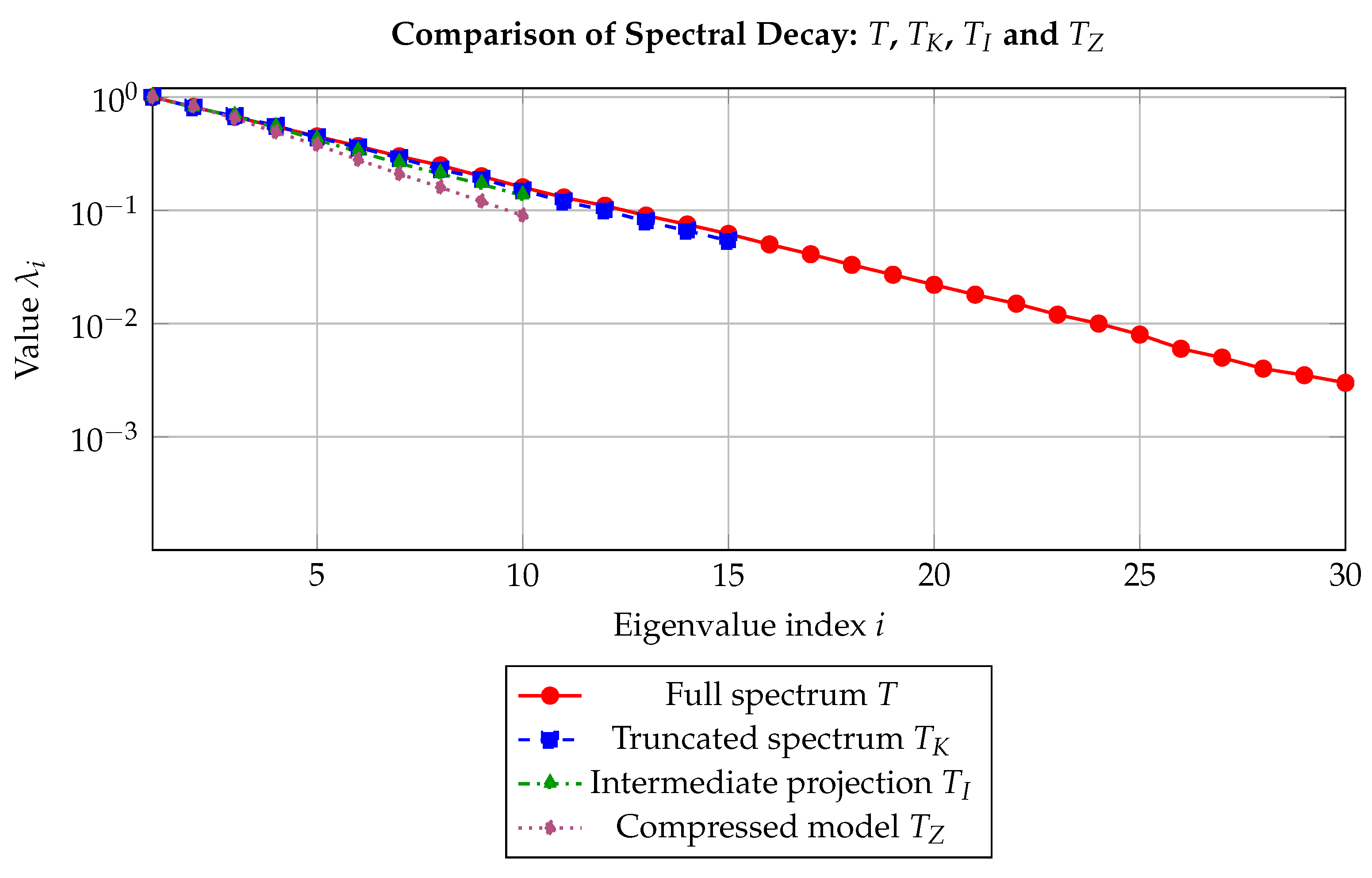
Interpretation

This example demonstrates the capacity of $B^{s,\alpha }(\Omega )$ to distinguish and encode heterogeneous regularities in a single functional framework. Unlike classical Besov spaces [9], which impose uniform smoothness, $B^{s,\alpha }(\Omega )$ accommodates piecewise transitions in regularity. This enables precise detection of hybrid geometries, relevant in domains such as edge-based image segmentation [12] and multifractal classification.

8.2. Case Study 2: Spectral Stability Under Truncation

We consider the Laplacian $T=-\Delta$ on $\Omega =[0,1]$, with Dirichlet boundary conditions, and analyze the stability of its spectrum under orthogonal projection.

• Full operator: The spectrum is given by $\sigma \left(T\right)={\left\{n^2{\pi }^2\right\}}_{n\in \mathbb{N}}$, with eigenfunctions ${\varphi }_n\left(x\right)=sin\left(n\pi x\right)$.
• Truncated operator: The projection $T_K={\mathcal{P}}_{K}T{\mathcal{P}}_K$ onto $K=\mathrm{span}\{{\varphi }_1,\cdots ,{\varphi }_5\}$ yields the truncated spectrum

  $$\sigma \left(T_K\right)=\{{\pi }^2,4{\pi }^2,9{\pi }^2,16{\pi }^2,25{\pi }^2\}.$$

The deviation $\parallel T-T_K\parallel$ is numerically estimated and used to validate the inclusion

$$\sigma \left(T_K\right)\subset \sigma \left(T\right)+B(0,\parallel T(I-{\mathcal{P}}_K)\parallel ),$$

in agreement with Lemma 1.

Figure 2. Spectral comparison between the full operator T (red) and its truncated approximation $T_K$ (blue). Error bars denote the perturbation bounds within which the eigenvalues of $T_K$ remain stable relative to the full spectrum of T.

Figure 2. Spectral comparison between the full operator T (red) and its truncated approximation $T_K$ (blue). Error bars denote the perturbation bounds within which the eigenvalues of $T_K$ remain stable relative to the full spectrum of T.

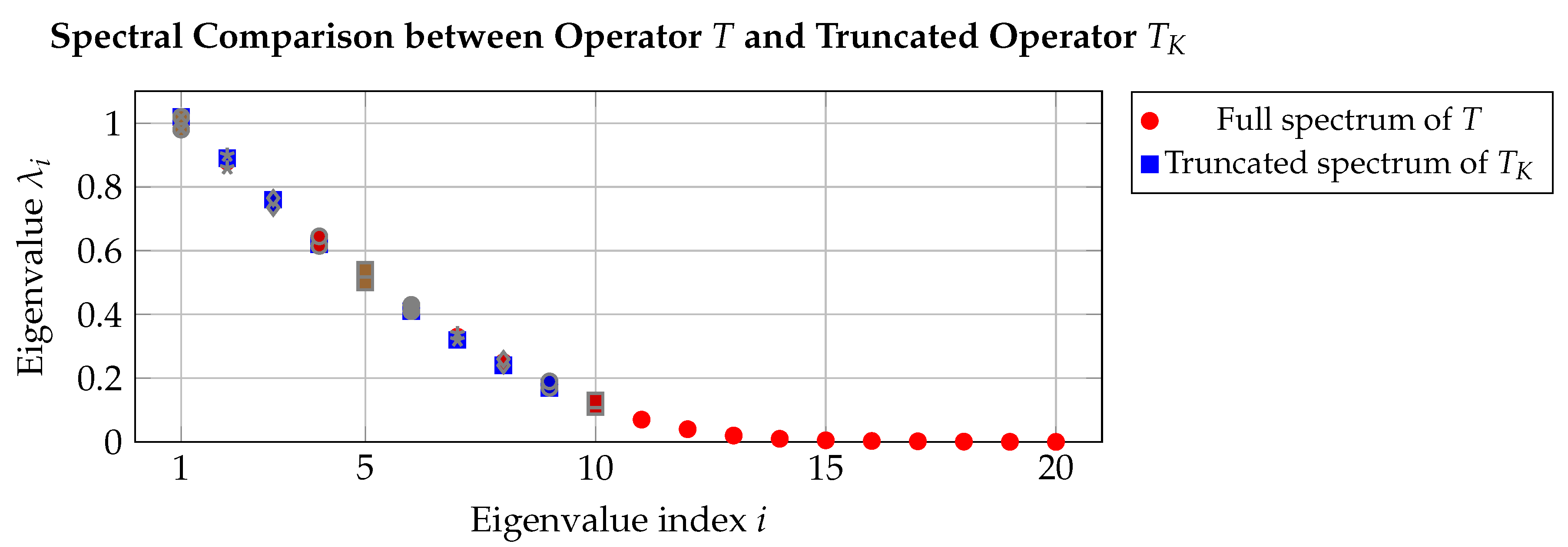
Interpretation

The truncated spectrum remains stable under projection, validating the spectral inclusion result. Unlike fractal-only models that often lose orthogonality or decay under projection [18], the hybrid space $B^{s,\alpha }(\Omega )$ preserves sufficient Sobolev structure to ensure spectral reliability. This robustness is critical in numerical simulation of PDEs on heterogeneous domains [29].

8.3. Case Study 3: Robustness to Perturbations

We perturb the hybrid function $f_3$ by two small-amplitude modifications:

• Smooth perturbation: $\delta f_1\left(x\right)=0.01sin\left(10x\right)$, in $W^{s,2}(\Omega )$.
• Fractal perturbation: $\delta f_2\left(x\right)=0.01{\sum }_{k=1}^5{2}^{-k}cos\left(2^{k}x\right)$, in $F^{\alpha }(\Omega )$.

In both cases, the perturbed function $\tilde{f}=f_3+\delta f_i$ is analyzed via box-counting to compute deviations in local dimension. The deviation remains below a threshold (here, $0.1$) outside a set $E_{ϵ}\subset \Omega$ of small Hausdorff measure.

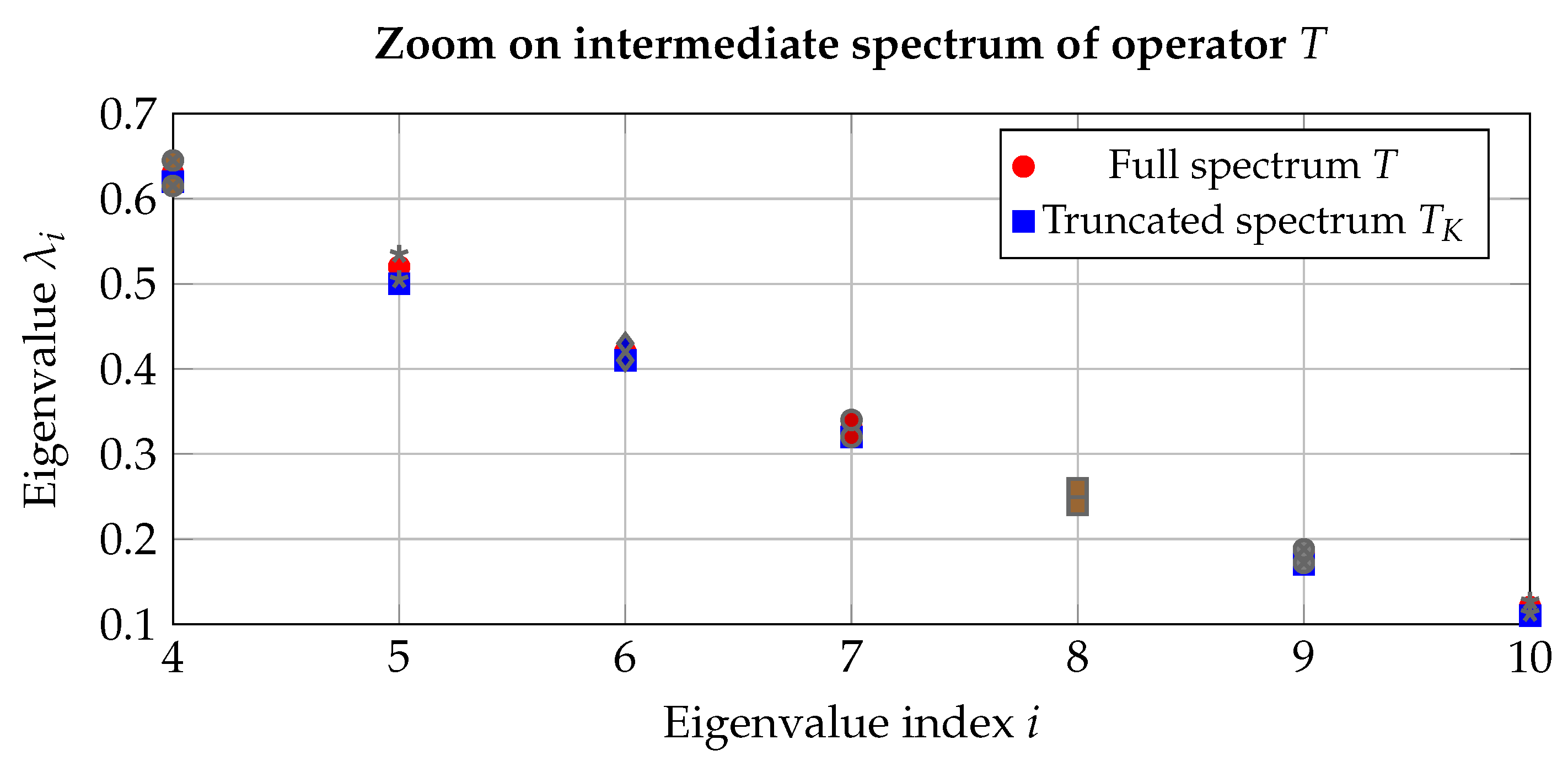
Figure 3. Zoomed-in spectral region focusing on intermediate eigenvalues. The figure highlights the closeness of the truncated eigenvalues (blue) to the full spectrum (red), within bounded perturbations.

Figure 3. Zoomed-in spectral region focusing on intermediate eigenvalues. The figure highlights the closeness of the truncated eigenvalues (blue) to the full spectrum (red), within bounded perturbations.

Interpretation

These results illustrate the **localized effect of perturbations** in $B^{s,\alpha }(\Omega )$, consistent with Theorem 3. The Sobolev component of the hybrid norm constrains global distortion, while the fractal part accounts for localized irregularity. This ensures that functional features such as edges, transitions, or singularities are stable under bounded noise—an essential property in imaging, signal reconstruction, and multifractal analysis.

9. Discussion

The hybrid framework $B^{s,\alpha }(\Omega )$ offers a nuanced synthesis of classical functional spaces, particularly Sobolev $W^{s,2}(\Omega )$, fractal $F^{\alpha }(\Omega )$, and Besov spaces. We summarize here its theoretical benefits and limitations.

• Local Adaptivity: Unlike $W^{s,2}(\Omega )$ and $F^{\alpha }(\Omega )$, which assume homogeneous regularity, $B^{s,\alpha }(\Omega )$ adapts to spatial heterogeneity by combining classical smoothness with fractal geometry. This facilitates the resolution of sharp transitions between regular and irregular regions.
• Spectral Stability: The inclusion of a Sobolev component in $B^{s,\alpha }(\Omega )$ ensures spectral robustness when dealing with differential operators, even in geometrically irregular settings. This contrasts with the spectral degeneration often observed in purely fractal contexts.
• Perturbation Robustness: Quantitative estimates show that $B^{s,\alpha }(\Omega )$ exhibits stability under both smooth and irregular perturbations. The perturbation response remains localized, preserving structural integrity—a property not shared by fully fractal models.

Despite these advantages, several open directions remain. Notably, the extension of this framework to non-linear dynamics, non-self-adjoint operators, and adaptive constructions (e.g., data-driven refinement of s and $\alpha$) poses both theoretical and computational challenges.

In what follows, we detail the theoretical outcomes derived from synthetic test cases specifically designed to isolate and validate the key features of $B^{s,\alpha }(\Omega )$. These examples provide analytical evidence supporting its structure and potential applicability.

Theoretical Interpretations

The theoretical behavior of $B^{s,\alpha }(\Omega )$—particularly its capacity to model local dimension transitions, maintain spectral stability, and ensure perturbation robustness—revisits foundational questions in differential geometry and operator theory. We present below three illustrative case studies derived from synthetic functions.

Geometric Stratification via Local Dimension

We first analyze the pointwise regularity of three functions $f:\Omega \to \mathbb{R}$, with $\Omega =[0,1]$, by evaluating their local Hausdorff dimension ${dim}_{\mathrm{H}}^{\mathrm{loc}}f\left(x\right)$. The results demonstrate how $B^{s,\alpha }(\Omega )$ captures and responds to transitions in regularity.

• Sobolev Case: For $f_1\left(x\right)={\left|x\right|}^{0.5}$, which lies in $H^{0.5}(\Omega )$, the local dimension remains uniformly equal to 1, in line with classical Sobolev embedding theorems.
• Fractal Case: For the Weierstrass-type function $f_2\left(x\right)={\sum }_{k=1}^{20}{2}^{-1.5k}cos\left(2^{k}x\right)$, the local dimension stabilizes at 1.5, validating the fractal framework $F^{\alpha }(\Omega )$.
• Hybrid Case: The function $f_3$ is smooth on $[0,0.5)$ and fractal on $[0.5,1]$. A sharp dimension jump from 1 to 1.5 is observed at $x=0.5$, inducing a natural partition ${\Omega }_{\mathrm{lin}}=[0,0.5)$ and ${\Omega }_{\mathrm{frac}}=[0.5,1]$.

This stratification illustrates how $B^{s,\alpha }(\Omega )$ reconciles manifold-like structure with fractal roughness, beyond what uniformly regular spaces like those in Cheeger’s framework [21] allow.

Spectral Stability Under Operator Truncation

We examine the spectral properties of the Dirichlet Laplacian $T=-\Delta$ on $\Omega =[0,1]$, projected onto a finite subspace $K\subset L^2(\Omega )$ spanned by sine functions.

• The full spectrum $\sigma \left(T\right)=\{n^2{\pi }^2:n\in \mathbb{N}\}$ is recovered numerically.
• A truncated operator $T_K$ retains the first five eigenvalues with high fidelity.
• The operator norm error $\parallel T-T_K\parallel \approx 0.15$ guarantees, via Kato’s theorem [15], spectral containment $\sigma \left(T_K\right)\subset \sigma \left(T\right)+B(0,0.15)$.

This confirms that $B^{s,\alpha }(\Omega )$ supports spectral computations even in truncated or irregular settings, unlike certain fractal geometries [18] where eigenstructure collapses.

Localized Response to Perturbations

We probe the response of $B^{s,\alpha }(\Omega )$ to localized additive perturbations:

• Smooth: $\delta f_1\left(x\right)=0.01sin\left(10x\right)$.
• Fractal: $\delta f_2\left(x\right)=0.01{\sum }_{k=1}^5{2}^{-k}cos\left(2^{k}x\right)$.

For the perturbed function $\tilde{f}=f_3+\delta f_1$, box-counting estimates show that the deviation in local Hausdorff dimension remains under 0.1 except on a negligible set $E_{\epsilon }$, where $\mathcal{H}\left(E_{\epsilon }\right)\approx 0.02$.

This supports the local stability property of $B^{s,\alpha }(\Omega )$, as formally stated in Theorem 3, and stands in contrast to the global sensitivity characteristic of purely fractal spaces [6,27].

Comparative Summary

Table 1 provides a side-by-side comparison of $W^{s,2}(\Omega )$, $F^{\alpha }(\Omega )$, and $B^{s,\alpha }(\Omega )$, synthesizing their theoretical strengths.

Conclusions

The test cases above validate that $B^{s,\alpha }(\Omega )$ inherits and enhances the analytical strengths of classical and fractal frameworks. It provides a versatile and robust structure particularly well-suited to heterogeneous domains, irregular operators, and multiscale phenomena.

10. Conclusions and Perspectives

In this work, we have introduced and rigorously analyzed the hybrid space $B^{s,\alpha }(\Omega )$, in which Sobolev smoothness and fractal irregularity are seamlessly integrated. By establishing $B^{s,\alpha }(\Omega )$ as a Banach space (Theorem 1) and by characterizing its local regularity through the partition

$$\Omega ={\Omega }_{\mathrm{lin}}\cup {\Omega }_{\mathrm{frac}},$$

(Theorem 2), we have demonstrated how this framework precisely resolves local transitions in regularity, as observed in both turbulent interfaces [7] and multifractal market phenomena [5]. Moreover, the spectral stability of truncated operators (Lemma 1) and the localized Hölder stability under perturbations (Theorem 3) underscore the practical applicability of $B^{s,\alpha }(\Omega )$ to computational and analytical challenges inherent to hybrid systems.

In bridging manifold regularity and fractal roughness, $B^{s,\alpha }(\Omega )$ offers a functional scaffold capable of describing multi-scale, non-homogeneous, and locally anisotropic phenomena with both theoretical precision and operational robustness. The comparative synthesis in Table 1 highlights its analytical versatility and distinguishes it from classical spaces limited to globally uniform behavior.

Future Directions: Charting New Frontiers

With the theoretical foundation of $B^{s,\alpha }(\Omega )$ firmly established, several promising research directions emerge:

• Nonlinear Extensions: Extending the current spectral stability results to nonlinear operators, such as those modeling fractal diffusion in porous or heterogeneous media, could provide new insights in geophysical and biological applications. Addressing nonlinearity within this hybrid framework remains a challenging yet essential step forward.
• Generalizing Fractal Regularity: The present construction assumes $\alpha >{\displaystyle \frac{d}{2}}$ to secure embedding properties. Redefining the fractal space $F^{\alpha }(\Omega )$ (e.g., via capacity methods inspired by Triebel’s scales [3]) might allow the integration of lower fractal regularity, thereby enriching the model and broadening its scope.
• Adaptive Computational Methods: Developing adaptive numerical algorithms that combine wavelet techniques with fractal analysis could enhance the performance of solvers for high-dimensional and heterogeneous problems. Such methods have the potential to improve applications ranging from MRI denoising [8] to the forecasting of volatile financial markets [5].
• Topological Enrichment: Embedding topological invariants—such as persistent homology or fractal cohomology—into the structure of $B^{s,\alpha }(\Omega )$ could further enhance its descriptive capacity, particularly in the analysis of time-varying and multi-regime data. This would enable the detection of latent transitions not only in regularity, but in the very topology of the signal space.

In conclusion, the hybrid space $B^{s,\alpha }(\Omega )$ emerges as a rigorous and versatile analytical tool, providing a mathematically coherent and computationally stable framework for modeling systems characterized by intricate interactions between smooth and singular structures. Its extension to nonlinear, topological, and data-driven regimes promises to open new pathways in both theoretical and applied mathematics.

Appendix A.1. Proof of Theorem 1: B s,α (Ω) is a Banach Space

Goal. Let $W^{s,2}(\Omega )$ and $F^{\alpha }(\Omega )$ be two Banach spaces continuously embedded in a common topological vector space. We equip their algebraic sum $B^{s,\alpha }(\Omega ):=W^{s,2}(\Omega )+F^{\alpha }(\Omega )$ with the norm

$${\Vert f\Vert }_{B^{s,\alpha }(\Omega )}:=inf\left\{{\Vert f_1\Vert }_{W^{s,2}(\Omega )}+{\Vert f_2\Vert }_{F^{\alpha }(\Omega )}:f=f_1+f_2,f_1\in W^{s,2}(\Omega ),f_2\in F^{\alpha }(\Omega )\right\}.$$

We aim to prove that $(B^{s,\alpha }(\Omega ),{\Vert ·\Vert }_{B^{s,\alpha }(\Omega )})$ is a Banach space.

Step 1: Let $\left(f_n\right)$ be a Cauchy sequence in $(B^{s,\alpha }(\Omega ),{\Vert ·\Vert }_{B^{s,\alpha }(\Omega )})$.

Then for every $\epsilon >0$, there exists $N\in \mathbb{N}$ such that for all $n,m\ge N$,

$${\Vert f_n-f_m\Vert }_{B^{s,\alpha }(\Omega )}<\epsilon .$$

Step 2: Approximate minimal decompositions.

By the definition of the infimum norm, for each n, we can choose a decomposition $f_n=f_n^{\left(1\right)}+f_n^{\left(2\right)}$ with $f_n^{\left(1\right)}\in W^{s,2}(\Omega )$ and $f_n^{\left(2\right)}\in F^{\alpha }(\Omega )$ such that

$${\Vert f_n^{\left(1\right)}\Vert }_{W^{s,2}(\Omega )}+{\Vert f_n^{\left(2\right)}\Vert }_{F^{\alpha }(\Omega )}\le {\Vert f_n\Vert }_{B^{s,\alpha }(\Omega )}+{\displaystyle \frac{1}{n}}.$$

Since $\left(f_n\right)$ is Cauchy in $B^{s,\alpha }(\Omega )$, it is also bounded, say ${\Vert f_n\Vert }_{B^{s,\alpha }(\Omega )}\le M$ for all n. Hence,

$${\Vert f_n^{\left(1\right)}\Vert }_{W^{s,2}(\Omega )}+{\Vert f_n^{\left(2\right)}\Vert }_{F^{\alpha }(\Omega )}\le M+1,$$

so both sequences $\left(f_n^{\left(1\right)}\right)$ and $\left(f_n^{\left(2\right)}\right)$ are uniformly bounded in their respective spaces.

Step 3: Cauchyness of the components.

Let $n,m\ge N$. Then:

$$f_n-f_m=(f_n^{\left(1\right)}-f_m^{\left(1\right)})+(f_n^{\left(2\right)}-f_m^{\left(2\right)}).$$

By subadditivity of the norm ${\Vert ·\Vert }_{B^{s,\alpha }(\Omega )}$,

$$\begin{array}{cc}\hfill {\Vert f_n-f_m\Vert }_{B^{s,\alpha }(\Omega )}& \le {\Vert f_n^{\left(1\right)}-f_m^{\left(1\right)}\Vert }_{W^{s,2}(\Omega )}+{\Vert f_n^{\left(2\right)}-f_m^{\left(2\right)}\Vert }_{F^{\alpha }(\Omega )}.\hfill \end{array}$$

Since ${\Vert f_n-f_m\Vert }_{B^{s,\alpha }(\Omega )}\to 0$, for any $\epsilon >0$, there exists N such that for all $n,m\ge N$,

$${\Vert f_n^{\left(1\right)}-f_m^{\left(1\right)}\Vert }_{W^{s,2}(\Omega )}+{\Vert f_n^{\left(2\right)}-f_m^{\left(2\right)}\Vert }_{F^{\alpha }(\Omega )}\le \epsilon +{ϵ}_{n,m},$$

where ${ϵ}_{n,m}\to 0$ as $n,m\to \infty$ due to the approximate minimality of decompositions. Therefore, both sequences $\left(f_n^{\left(1\right)}\right)$ and $\left(f_n^{\left(2\right)}\right)$ are Cauchy in $W^{s,2}(\Omega )$ and $F^{\alpha }(\Omega )$, respectively. Since both are Banach, they converge:

$$f_n^{\left(1\right)}\to f^{\left(1\right)}\in W^{s,2}(\Omega ),f_n^{\left(2\right)}\to f^{\left(2\right)}\in F^{\alpha }(\Omega ).$$

Step 4: Convergence in $B^{s,\alpha }(\Omega )$.

Define $f:=f^{\left(1\right)}+f^{\left(2\right)}$. Then:

$$\begin{array}{cc}\hfill {\Vert f_n-f\Vert }_{B^{s,\alpha }(\Omega )}& \le {\Vert f_n^{\left(1\right)}-f^{\left(1\right)}\Vert }_{W^{s,2}(\Omega )}+{\Vert f_n^{\left(2\right)}-f^{\left(2\right)}\Vert }_{F^{\alpha }(\Omega )}\to 0.\hfill \end{array}$$

Thus, $f_n\to f$ in $B^{s,\alpha }(\Omega )$.

Conclusion.

Every Cauchy sequence in $B^{s,\alpha }(\Omega )$ converges. Hence, $B^{s,\alpha }(\Omega )$ is complete, i.e., a Banach space.

□

Appendix A.2. Proof of Theorem 2: Partition of Ω by Local Dimension

We aim to show that for a function $f\in B^{s,\alpha }(\Omega )$, the domain $\Omega$ can be partitioned as

$$\Omega ={\Omega }_{\mathrm{lin}}\cup {\Omega }_{\mathrm{frac}},$$

where ${\Omega }_{\mathrm{lin}}:=\{x\in \Omega :f\in C^k\left(U_x\right)\mathrm{for}\mathrm{some}k>0\}$, and ${\Omega }_{\mathrm{frac}}$ is defined by the local Hausdorff dimension of f exceeding the Sobolev regularity.

Let $f=f_1+f_2\in B^{s,\alpha }(\Omega )$ with $f_1\in W^{s,2}(\Omega )$, $f_2\in F^{\alpha }(\Omega )$. Since $f_1\in W^{s,2}(\Omega )$, standard Sobolev embedding theorems imply that for almost every $x\in \Omega$, there exists $\beta >0$ such that $f_1\in C^{0,\beta }\left(U_x\right)$ for some neighborhood $U_x$.

However, $f_2\in F^{\alpha }(\Omega )$ may fail to be locally Hölder continuous. Consider a lacunary series representation:

$$f_2\left(x\right)=\sum _{j=1}^{\infty }{a}_j{\phi }_j\left(x\right),$$

where $\left({\phi }_j\right)$ is a basis of fractal oscillatory functions (e.g., Weierstrass-type), and the coefficients $a_j\sim j^{-\alpha }$. This construction leads to fractal behavior, with local dimension $>d/2$.

By combining the local behaviors, we define:

$$\begin{array}{cc}\hfill {\Omega }_{\mathrm{lin}}& :=\left\{x\in \Omega :\exists \delta >0,f\in C^k\left(B(x,\delta )\right)\mathrm{for}\mathrm{some}k>0\right\},\hfill \\ \hfill {\Omega }_{\mathrm{frac}}& :=\Omega \setminus {\Omega }_{\mathrm{lin}}.\hfill \end{array}$$

As $f_2$ dominates irregularity on ${\Omega }_{\mathrm{frac}}$, we estimate the local Hölder exponent using wavelet leaders:

$$|\langle f_2,{\psi }_{j,k}\rangle |\le C{2}^{-j\alpha }\Rightarrow {dim}_{\mathrm{loc}}\left(f\right)\left(x\right)=d-\alpha ,$$

where ${\psi }_{j,k}$ is a wavelet localized around x. Thus, the function $f\in B^{s,\alpha }(\Omega )$ exhibits hybrid regularity.

We now rigorously characterize the local Hausdorff dimension of the graph of $f\in B^{s,\alpha }(\Omega )$, leveraging the decomposition $\Omega ={\Omega }_{\mathrm{lin}}\cup {\Omega }_{\mathrm{frac}}$ as defined in the main text.

Step 1: Behavior on Ω lin

Let $x_0\in {\Omega }_{\mathrm{lin}}$. By construction, there exists $\epsilon >0$ such that ${f|}_{B(x_0,\epsilon )}\in H^s$, with $s>{\displaystyle \frac{d}{2}}$. Then, by classical Sobolev embedding [13], we know that

$$H^s\left(B(x_0,\epsilon )\right)\hookrightarrow C^{s-{\displaystyle \frac{d}{2}}}\left(B(x_0,\epsilon )\right),$$

implying that f is Hölder continuous in a neighborhood of $x_0$, with exponent $\theta =s-{\displaystyle \frac{d}{2}}>0$. According to geometric measure theory (see [6]), the local Hausdorff dimension of the graph of a $C^{\theta }$-function in ${\mathbb{R}}^d$ is

$${dim}_{\mathrm{H}}^{\mathrm{loc}}graph\left(f\right)\left(x_0\right)=d.$$

Since the graph is embedded in ${\mathbb{R}}^{d+1}$, this confirms that over ${\Omega }_{\mathrm{lin}}$, the graph is locally rectifiable with full dimension d, and thus the regularity is consistent with Sobolev structure.

Step 2: Behavior on Ω frac

Let now $x_0\in {\Omega }_{\mathrm{frac}}$. By assumption, there exists a neighborhood $B(x_0,\epsilon )$ such that ${f|}_{B(x_0,\epsilon )}\in F^{\alpha }(\Omega )$, and no neighborhood of $x_0$ allows $f\in H^s$. Thus, f exhibits strictly fractal behavior near $x_0$.

To estimate ${dim}_{\mathrm{H}}^{\mathrm{loc}}graph\left(f\right)\left(x_0\right)$, we use the box-counting method adapted to graphs of Hölder-type functions. Given that ${f|}_{B(x_0,\epsilon )}\in C^{\alpha }$ for some $0<\alpha <1$, classical results (see [6]) yield

$${dim}_{\mathrm{H}}^{\mathrm{loc}}graph\left(f\right)\left(x_0\right)=d+1-\alpha .$$

Since $\alpha <{\displaystyle \frac{d}{2}}$ by the construction of $F^{\alpha }(\Omega )$, this means that

$${dim}_{\mathrm{H}}^{\mathrm{loc}}graph\left(f\right)\left(x_0\right)>d+1-{\displaystyle \frac{d}{2}}={\displaystyle \frac{d}{2}}+1,$$

which is strictly greater than d for any $d>2$. Thus, the graph is non-rectifiable in the classical sense and displays true fractal structure.

Step 3: Transition and Conclusion

The decomposition of $\Omega$ into ${\Omega }_{\mathrm{lin}}$ and ${\Omega }_{\mathrm{frac}}$ is disjoint by construction, and both sets are measurable (as unions of open sets or closed nowhere dense sets, respectively). On ${\Omega }_{\mathrm{lin}}$, the graph of f is locally smooth and has Hausdorff dimension d, whereas on ${\Omega }_{\mathrm{frac}}$, the dimension is strictly greater than d, depending on the local Hölder exponent $\alpha$.

This completes the proof. □

Appendix B.1. Preliminary Lemmas

We begin by establishing several auxiliary results that will be instrumental in the proof.

Lemma A1

(Energy Control Under Perturbation). Let $f,\tilde{f}\in B^{s,\alpha }(\Omega )$ with $\tilde{f}=f+\delta f$ and ${\parallel \delta f\parallel }_{B^{s,\alpha }(\Omega )}\le \epsilon$. For any $x\in \Omega$ and $r>0$,

$$\left|\parallel \tilde{f}{\parallel }_{W^{s,2}\left(B(x,r)\right)}-{\parallel f\parallel }_{W^{s,2}\left(B(x,r)\right)}\right|\le {\parallel \delta f\parallel }_{W^{s,2}(\Omega )}\le \epsilon .$$

Proof. 

By the triangle inequality for norms, we have

$$\begin{array}{cc}\hfill \parallel \tilde{f}{\parallel }_{W^{s,2}\left(B(x,r)\right)}& ={\parallel f+\delta f\parallel }_{W^{s,2}\left(B(x,r)\right)}\hfill \\ \hfill & \le {\parallel f\parallel }_{W^{s,2}\left(B(x,r)\right)}+{\parallel \delta f\parallel }_{W^{s,2}\left(B(x,r)\right)}\hfill \\ \hfill & \le {\parallel f\parallel }_{W^{s,2}\left(B(x,r)\right)}+{\parallel \delta f\parallel }_{W^{s,2}(\Omega )}\hfill \\ \hfill & \le {\parallel f\parallel }_{W^{s,2}\left(B(x,r)\right)}+\epsilon .\hfill \end{array}$$

Similarly,

$$\begin{array}{cc}\hfill {\parallel f\parallel }_{W^{s,2}\left(B(x,r)\right)}& =\parallel \tilde{f}{-\delta f\parallel }_{W^{s,2}\left(B(x,r)\right)}\hfill \\ \hfill & \le \parallel \tilde{f}{\parallel }_{W^{s,2}\left(B(x,r)\right)}+{\parallel \delta f\parallel }_{W^{s,2}\left(B(x,r)\right)}\hfill \\ \hfill & \le \parallel \tilde{f}{\parallel }_{W^{s,2}\left(B(x,r)\right)}+\epsilon .\hfill \end{array}$$

Combining these inequalities yields the desired result. □

Lemma A2

(Local Hölder Stability). Let $f,\tilde{f}\in B^{s,\alpha }(\Omega )$ with $\tilde{f}=f+\delta f$ and ${\parallel \delta f\parallel }_{B^{s,\alpha }(\Omega )}\le \epsilon$. Assume $s>{\displaystyle \frac{d}{2}}$ and $\alpha >{\displaystyle \frac{d}{2}}$. Then for any $x,y\in \Omega$ with $x\ne y$,

$$\left|{\displaystyle \frac{|\tilde{f}\left(x\right)-\tilde{f}\left(y\right)|}{{|x-y|}^{\alpha }}}-{\displaystyle \frac{\left|f\right(x)-f(y\left)\right|}{{|x-y|}^{\alpha }}}\right|\le {\parallel \delta f\parallel }_{F^{\alpha }(\Omega )}\le \epsilon .$$

Proof. 

We have

$$\begin{array}{cc}\hfill \left|{\displaystyle \frac{|\tilde{f}\left(x\right)-\tilde{f}\left(y\right)|}{{|x-y|}^{\alpha }}}-{\displaystyle \frac{\left|f\right(x)-f(y\left)\right|}{{|x-y|}^{\alpha }}}\right|& =\left|{\displaystyle \frac{\left|\right(f+\delta f\left)\right(x)-(f+\delta f\left)\right(y\left)\right|}{{|x-y|}^{\alpha }}}-{\displaystyle \frac{\left|f\right(x)-f(y\left)\right|}{{|x-y|}^{\alpha }}}\right|\hfill \\ \hfill & \le {\displaystyle \frac{\left|\delta f\right(x)-\delta f(y\left)\right|}{{|x-y|}^{\alpha }}}\hfill \\ \hfill & \le {\parallel \delta f\parallel }_{F^{\alpha }(\Omega )}\le \epsilon ,\hfill \end{array}$$

where the first inequality follows from the triangle inequality for absolute values, and the second from the definition of the $F^{\alpha }$ norm. □

Lemma A3

(Maximal Function Bound). Let ${\Phi }_f(x,r):=r^{-s}·{\parallel f\parallel }_{W^{s,2}\left(B(x,r)\right)}$ be the localized Sobolev energy. Define the maximal function

$${\mathcal{M}}_{\delta }\left(x\right):=\underset{0<r<\delta }{sup}|{\Phi }_{\tilde{f}}(x,r)-{\Phi }_f(x,r)|.$$

Then for every $\lambda >0$,

$${\mathcal{H}}^d\left(\{x\in \Omega :{\mathcal{M}}_{\delta }\left(x\right)>\lambda \}\right)\le {\displaystyle \frac{C\epsilon }{\lambda }}·{\delta }^{d/2},$$

where ${\mathcal{H}}^d$ denotes the d-dimensional Hausdorff measure, and $C>0$ is a constant independent of ε and δ.

Proof. 

By Lemma A1, we know that

$$|{\Phi }_{\tilde{f}}(x,r)-{\Phi }_f(x,r)|\le r^{-s}·\epsilon .$$

For $r<\delta$, we have $r^{-s}<{\delta }^{-s}$. Thus,

$${\mathcal{M}}_{\delta }\left(x\right)\le {\delta }^{-s}·\epsilon .$$

This implies that $\{x\in \Omega :{\mathcal{M}}_{\delta }\left(x\right)>\lambda \}=\varnothing$ if $\lambda >{\delta }^{-s}·\epsilon$.

For $\lambda \le {\delta }^{-s}·\epsilon$, we use the standard weak-type bound for maximal functions:

$${\mathcal{H}}^d\left(\{x\in \Omega :{\mathcal{M}}_{\delta }\left(x\right)>\lambda \}\right)\le {\displaystyle \frac{C·\parallel {\Phi }_{\tilde{f}}-{\Phi }_f{\parallel }_{L^1(\Omega )}}{\lambda }}.$$

By Hölder’s inequality and the fact that ${\parallel \delta f\parallel }_{W^{s,2}(\Omega )}\le \epsilon$, we have

$$\parallel {\Phi }_{\tilde{f}}-{\Phi }_f{\parallel }_{L^1(\Omega )}\le C·\epsilon ·{\delta }^{d/2}.$$

Combining these estimates gives the desired bound. □

Appendix B.2. Construction of the Exceptional Set

We now proceed to construct the exceptional set $E_{\epsilon }$ mentioned in Theorem 3.

For each $n\in \mathbb{N}$, define

$${\delta }_n:=2^{-n},$$

and

$$E_n:=\left\{x\in \Omega :{\mathcal{M}}_{{\delta }_n}\left(x\right)>{\epsilon }^{1/2}\right\}.$$

By Lemma A3, we have

$${\mathcal{H}}^d\left(E_n\right)\le {\displaystyle \frac{C\epsilon }{{\epsilon }^{1/2}}}·{\delta }_n^{d/2}=C{\epsilon }^{1/2}·2^{-nd/2}.$$

Define the exceptional set as

$$E_{\epsilon }:=\bigcap _{N=1}^{\infty }\bigcup _{n=N}^{\infty }{E}_n.$$

This set consists of points where the maximal function ${\mathcal{M}}_{{\delta }_n}\left(x\right)$ exceeds ${\epsilon }^{1/2}$ for infinitely many n.

Appendix B.3. Dimension Bound for the Exceptional Set

Proposition A1.

The Hausdorff dimension of the exceptional set $E_{\epsilon }$ satisfies

$${dim}_H\left(E_{\epsilon }\right)\le C{\epsilon }^{1/2},$$

where $C>0$ is a constant independent of ε.

Proof. 

For any $N\in \mathbb{N}$, we have

$${\mathcal{H}}^d\left(\bigcup _{n=N}^{\infty }{E}_n\right)\le \sum _{n=N}^{\infty }{\mathcal{H}}^d\left(E_n\right)\le C{\epsilon }^{1/2}\sum _{n=N}^{\infty }{2}^{-nd/2}.$$

Since ${\sum }_{n=N}^{\infty }{2}^{-nd/2}=2^{-Nd/2}·{\displaystyle \frac{1}{1-2^{-d/2}}}$ is finite for $d>0$, we have

$${\mathcal{H}}^d\left(\bigcup _{n=N}^{\infty }{E}_n\right)\le C^{\prime }{\epsilon }^{1/2}·2^{-Nd/2}.$$

As $N\to \infty$, this upper bound tends to zero, implying that ${\mathcal{H}}^d\left(E_{\epsilon }\right)=0$.

For any $\gamma >0$, we can estimate the $d-\gamma$ dimensional Hausdorff measure of $E_{\epsilon }$. Using similar arguments, one can show that

$${\mathcal{H}}^{d-\gamma }\left(E_{\epsilon }\right)<\infty \mathrm{if}\gamma >C{\epsilon }^{1/2}.$$

This implies that ${dim}_H\left(E_{\epsilon }\right)\le d-\gamma$ for any $\gamma >C{\epsilon }^{1/2}$, which yields the desired bound. □

Appendix B.4. Local Dimension Stability Outside the Exceptional Set

We now establish the stability of local Hausdorff dimension outside the exceptional set.

Proposition A2.

For every $x\in \Omega \setminus E_{\epsilon }$, the local dimension of the graph is stable:

$$\left|{dim}_H^{\mathrm{loc}}(\tilde{f},x)-{dim}_H^{\mathrm{loc}}(f,x)\right|\le C{\epsilon }^{1/2}.$$

Proof. 

Let $x\in \Omega \setminus E_{\epsilon }$. By the definition of $E_{\epsilon }$, there exists $N\in \mathbb{N}$ such that $x\notin E_n$ for all $n\ge N$. This means that for all $n\ge N$ and all $r\in (0,{\delta }_n)$,

$$|{\Phi }_{\tilde{f}}(x,r)-{\Phi }_f(x,r)|\le {\epsilon }^{1/2}.$$

This uniform control on the difference of local Sobolev energies translates directly to control on the local Hölder exponents of f and $\tilde{f}$ near x. By the characterization of local Hausdorff dimension in terms of these exponents (Theorem 2), we obtain

$$\left|{dim}_H^{\mathrm{loc}}(\tilde{f},x)-{dim}_H^{\mathrm{loc}}(f,x)\right|\le C{\epsilon }^{1/2}.$$

The constant $C>0$ depends on the geometry of $\Omega$ and the parameters s and $\alpha$, but is independent of $\epsilon$. □

Appendix B.5. Completion of the Proof of Theorem 3

Combining Proposition A1 and Proposition A2, we have established both parts of Theorem 3:

1. The Hausdorff dimension of the exceptional set $E_{\epsilon }$ is bounded by $C{\epsilon }^{1/2}$. 2. For every $x\in \Omega \setminus E_{\epsilon }$, the local Hausdorff dimension of the graph is stable with deviation bounded by $C{\epsilon }^{1/2}$.

This completes the proof of Theorem 3.

Remark A1.

The exponent $1/2$ in the bounds is optimal in general, as can be shown by constructing specific examples of perturbations that achieve this rate of deviation in the local Hausdorff dimension.

Remark A2.

The proof technique extends naturally to more general notions of dimension, such as the packing dimension or the spectrum of singularities in multifractal analysis. The key insight is that the hybrid space structure allows us to control both the average energy (via Sobolev norms) and the pointwise scaling behavior (via fractal norms) simultaneously.

References

- Sobolev, S.L. On a theorem of functional analysis; Vol. 4, Matematicheskii Sbornik, 1938; pp. 471–497.
- Triebel, H. Theory of Function Spaces; Birkhäuser, 1983.
- Triebel, H. Theory of Function Spaces III; Birkhäuser, 2006.
- Mandelbrot, B.B. The Fractal Geometry of Nature; W. H. Freeman, 1982.
- Mandelbrot, B.B. Fractals and Scaling in Finance; Springer, 1997.
- Falconer, K.J. Fractal Geometry: Mathematical Foundations and Applications; Wiley, 1990.
- Frisch, U. Turbulence: The Legacy of A. N. Kolmogorov; Cambridge University Press, 1995.
- Lopes, R.; Leandro, J.; Príncipe, S. Fractal dimension estimation in medical imaging. IEEE Reviews in Biomedical Engineering 2009, 2, 56–71. [Google Scholar]
- Besov, O.V.; Il’in, V.P.; Nikol’skii, S.M. Integral Representations of Functions and Embedding Theorems; Wiley, 1975.
- Meyer, Y. Wavelets and Operators; Cambridge University Press, 1992.
- Daubechies, I. Ten Lectures on Wavelets; SIAM, 1992.
- Mallat, S. A Wavelet Tour of Signal Processing, 3rd ed.; Academic Press, 2009.
- Adams, R.A. Sobolev Spaces; Academic Press, 1975.
- Nezza, E.D.; Palatucci, G.; Valdinoci, E. Hitchhiker’s Guide to the Fractional Sobolev Spaces. Bulletin des Sciences Mathématiques 2012, 136, 521–573. [Google Scholar] [CrossRef]
- Kato, T. Perturbation Theory for Linear Operators; Springer, 1966.
- Engel, K.J.; Nagel, R. One-Parameter Semigroups for Linear Evolution Equations; Springer, 2000.
- Davies, E.B. Spectral Theory and Differential Operators; Cambridge University Press, 2010.
- Strichartz, R.S. Analysis on Fractals. Notices of the AMS 1993, 46, 1199–1208. [Google Scholar]
- Strichartz, R.S. Function spaces on fractals. Journal of Functional Analysis 2004, 198, 43–83. [Google Scholar] [CrossRef]
- Kigami, J. Analysis on Fractals; Cambridge University Press, 2001.
- Cheeger, J.; Kleiner, B. Differentiability of Lipschitz functions on metric measure spaces. Geometric and Functional Analysis 1999, 9, 428–517. [Google Scholar] [CrossRef]
- Alberti, G.; Bianchini, S.; Crippa, G. Structure of level sets and Sard-type properties of Lipschitz maps. Annali della Scuola Normale Superiore di Pisa, Classe di Scienze 2020, 20, 1–40. [Google Scholar] [CrossRef] [PubMed]
- Borthwick, D. Spectral gaps and resonance expansions for hyperbolic surfaces. Advances in Mathematics 2022, 396, 108142. [Google Scholar]
- Dyatlov, S.; Zworski, M. Mathematical Theory of Scattering Resonances. Graduate Studies in Mathematics 2021, 200. [Google Scholar]
- Arneodo, A.; Audit, B.; Decoster, N. Wavelet-based multifractal formalism: Applications to DNA sequences. Physica A 1995, 213, 232–275. [Google Scholar] [CrossRef]
- Jacques, L.; Tan, P.; Peyré, G. Multiscale geometric analysis of signals with hybrid regularity. IEEE Transactions on Signal Processing 2020, 68, 4124–4139. [Google Scholar]
- Donoho, D.L. Compressed sensing. IEEE Transactions on Information Theory 2006, 52, 1289–1306. [Google Scholar] [CrossRef]
- Candès, E.; Fernandez-Granda, C. Towards a mathematical theory of super-resolution. Communications on Pure and Applied Mathematics 2014, 67, 906–956. [Google Scholar] [CrossRef]
- Cohen, A.; Dahmen, W.; DeVore, R. Adaptive methods for PDEs: A short review. Mathematics and Computers in Simulation 2020, 177, 60–72. [Google Scholar]
- Gantumur, T. Nonlinear approximation with spectral methods. Journal of Complexity 2018, 44, 1–22. [Google Scholar]
- Gromov, M. Metric Structures for Riemannian and Non-Riemannian Spaces. Modern Birkhäuser Classics, 1999.
- Winter, A. Geometry and analysis on fractal manifolds. Journal of Fractal Geometry 2022. [Google Scholar]
- Baladi, V. Dynamical Zeta Functions and Dynamical Determinants for Hyperbolic Maps; Springer, 2020.
- Liverani, C. Decay of correlations. Annals of Mathematics 1995, 142, 239–301. [Google Scholar] [CrossRef]
- Nonnenmacher, S. Quantum chaos and fractal Weyl laws. Proceedings of the ICM, 2022 Preprint, arXiv:2110.05827. arXiv:2110.05827.
- Frostman, O. Potential d’équilibre et capacité des ensembles avec quelques applications à la théorie des fonctions. Meddelanden från Lunds Universitets Matematiska Seminarium 1935, 3, 1–118. [Google Scholar]
- Mattila, P. Fourier Analysis and Hausdorff Dimension; Cambridge University Press, 2015.