
Submitted:
07 March 2025
Posted:
10 March 2025
You are already at the latest version
Abstract
Functional data, including one-dimensional curves and higher-dimensional surfaces, have become increasingly prominent across scientific disciplines.
They offer a continuous perspective that captures subtle dynamics and richer structures compared to discrete representations, thereby preserving essential information and facilitating more natural modeling of real-world phenomena, especially in sparse or irregularly sampled settings.
A key challenge lies in identifying low-dimensional representations and estimating covariance structures that capture population statistics effectively.
We propose a novel Bayesian framework with a nonparametric kernel expansion and a sparse prior, enabling direct modeling of measured data and avoiding the artificial biases from regridding.
Our method, Bayesian scalable functional data analysis (BSFDA), automatically selects both subspace dimensionalities and basis functions, reducing computational overhead through an efficient variational optimization strategy.
We further propose a faster approximate variant that maintains comparable accuracy but accelerates computations significantly on large-scale datasets.
Extensive simulation studies demonstrate that our framework outperforms conventional techniques in covariance estimation and dimensionality selection, showing resilience to high dimensionality and irregular sampling.
The proposed methodology proves effective for multidimensional functional data and showcases practical applicability in biomedical and meteorological datasets.
Overall, BSFDA offers an adaptive, continuous, and scalable solution for modern functional data analysis across diverse scientific domains.
Keywords:
Functional data analysis
; Principal component analysis
; Dimension reduction
; Sparse Bayesian learning
; Variational Bayesian inference
; Nonparametric methods
; Model selection
1. Introduction
The emergence of big data across diverse fields, such as biomedicine, finance, and physical modeling, has catalyzed the need for advanced analytical methodologies capable of handling complex, high-dimensional datasets that conventional discrete-data analysis approaches cannot always process effectively. Such datasets often require analysis that captures and interprets their continuous and potentially high-dimensional complexities–a central promise of functional data analysis (FDA) [1,2]. Foundational work established FDA’s capacity to treat each observation as an entire function [3], be it a curve, surface, or higher-dimensional structure, thereby extracting richer insights than conventional discrete-point analyses. Over the past decade, FDA’s scope has widened significantly to accommodate high-dimensional and multivariate applications with theoretical and computational advances emerging across various contexts [4,5,6].
A pivotal technique within FDA is functional principal component analysis (fPCA), which serves as a dimension-reduction tool similar to classical PCA and factor analysis. Unlike classical PCA, however, fPCA operates in principle in an infinite-dimensional function space to capture dominant modes of variation and reduce complexity [7]. Despite its conceptual elegance, existing fPCA and similar FDA models often assume that data is observed on a shared, finite grid, often relying on heuristic imputation or posterior estimation to handle any missing entries [8,9,10,11,12,13,14,15,16,17,18]. This assumption conveniently facilitates the adoption of established linear algebraic methods, but compromises the integrity of FDA by introducing significant information loss and high computational demands in high-dimensional applications.
Ideally, each function would be represented according to its naturally sampled measurement points rather than forcing all observations onto a shared grid, thus preserving crucial information and avoiding the need for heuristic resampling. This point is critical when considering that, given only a finite number of data points, infinitely many functions can interpolate these points, each reflecting different inductive biases about smoothness or shape [19]. Conventional smoothing or regridding methods (e.g., polynomial interpolation) introduce biases that may distort the underlying function’s actual behavior. In contrast, we will achieve more accurate and unbiased predictions by concurrently updating the function estimation and the population-level statistics governing the estimation, such as those encoded in the covariance operator. Such an approach requires directly modeling the function from its original measurement points rather than imposing artificial grids.
To mitigate these limitations, several studies have proposed alternative strategies. For instance, [3] developed a nonparametric technique for estimating mean and covariance for functional data under smoothness assumptions while also discussing a continuous formulation and the necessary discretization in practical applications. In [20,21], they extended fPCA to sparse and irregular longitudinal designs by smoothing the covariance estimate and then discretizing. Nonetheless, classical discretization steps often result in significant information loss and computational burdens.
As functional data size and complexity grew, researchers turned to flexible basis expansions, including sinusoids (Fourier), wavelets, polynomials, and B-splines, for a finite-dimensional representation of functional data that is convenient and accurate in computation, avoiding the drawbacks of explicit approximation and resampling [2,22,23,24,25,26]. For example, [27] utilized basis function approximations to manage irregular grids. However, a core challenge remains in selecting a suitable model. For instance, researchers must choose the number and form (e.g., smoothness), along with the dimensionality of the representational subspace. In approximation, the placement of basis functions is also essential. Evenly spaced nodes remain popular for their simplicity but may be suboptimal. Alternative node allocations may be better, like Chebyshev nodes for superior accuracy [28], or sparse grids to reduce combinatorial growth of computational complexities [29].
Existing studies tend to rely on choosing the hyperparameters manually [7,10,11,30], or cross-validation [3,25,31,32], which are known to be computationally prohibitive. Others employ approximated cross-validation [22,24] or marginal likelihood [14] but still require exhaustive testing of all candidate models. Methods with sparse Bayesian priors [8,33,34] for model selection allow model selection with a single optimization. In [35,36], they use shrinkage or sparse priors for data-adaptive basis selection to ensure minimal but effective sets of basis functions. Notably, [37] proposed Bayesian and Akaike information criterion demonstrating state-of-the-art performance in simulation studies for sparse and dense functional data.
In addition, probabilistic FDA emerges as a sophisticated adaptation of probabilistic methods tailored to incorporate the flexibility of latent variable models to manage functional data. A Bayesian latent factor regression model (LFRM) [34], for example, extends conventional regression to accommodate complex structures and dependencies in functional data, providing a robust framework to handle the complexities inherent in functional data. However, these Bayesian approaches are often limited with the computational demands of Monte Carlo methods in high dimensions [14]. To address increasingly high-dimensional FDA problems, recent efforts have emphasized scalability. For instance, [7,30,38,39] introduced FDA for 2D and 3D images with a fixed basis or grid. In [32], they further reduced complexity in 2D fPCA via tensor product B-splines. And [40] applied a Bayesian framework with basis expansion, adaptive regularization, and Gibbs sampling to 2D functional data in the form of EEG studies on children with autism. Further, [41] leverages a parsimonious basis representation and variational Bayes to achieve computational efficiency, making it suitable for 3-D brain imaging data.
In parallel, the broader field of principal component analysis (PCA) remains a fundamental and effective tool. Classical PCA, rooted in eigen-decomposition [42], effectively extracts dominant modes of variation in many settings but does not inherently accommodate the probabilistic nature of real-world data and its inherent uncertainties. Thus, [43] introduced probabilistic PCA (PPCA), which incorporates a probability distribution to manage these uncertainties more effectively. PCA has since evolved to address missing data, model selection, and complex data types [44,45,46,47]. In the context of functional data, these concepts motivate new approaches that unify probabilistic methodologies, latent factor models, and kernel expansions for continuous domains [1].
Within Bayesian machine learning, various priors have been proposed for sparse or robust formulations of PCA [48,49,50,51]. Specifically, sparse Bayesian learning (SBL) [52,53,54] with its mechanism automatic relevance determination (ARD) [55,56] has proven adept at promoting parsimonious solutions [57,58,59,60,61]. SBL has emerged in Bayesian PCA [45,62,63], applying an iterative method to evaluate the relevance of each component and select the internal dimensionality by disregarding the redundant ones. [64] applied SBL to optimize the combination of base kernels to enhance model performance. These methods often exploit variational techniques or accelerated optimization [17,64,65,66,67,68,69,70], thereby balancing model complexity with computational tractability. In functional data contexts, where representations are infinite-dimensional, SBL offers a compelling framework for advanced FDA methods by efficiently handling sparse expansions and adaptively adjusting model complexity.
In summary, despite these efforts to advance functional data analysis, several challenges persist. Existing methods often exhibit limitations in accuracy and efficiency when sampling is sparse, automatic model selection is essential, and dimensionality is high [41]. Concurrently, probabilistic PCA and SBL frameworks illustrate powerful strategies to incorporate versatility and adaptivity for such data complexities while their adaptation to FDA is still evolving. These gaps underscore a need for a robust, flexible, and computationally feasible approach, unifying ideas from FDA, PPCA, and SBL, that manages the continuous and high-dimensional intricacy of modern datasets.
1.1. Contriubutions
This manuscript proposes a novel Bayesian framework for functional principal component analysis that leverages nonparametric kernel expansions, sparse Bayesian learning for model selection, and efficient variational inference (VI). We abbreviate the proposed method as BSFDA (Bayesian Scalable Functional Data Analysis). BSFDA addresses critical gaps in existing FDA techniques with irregular sampling, high-dimensional scalability, and selection of both basis functions and principal components. Specifically, our approach offers:
- Joint selection of optimum latent factors and sparse basis functions: This eliminates constraints on parametric representation dimensionality, avoids information loss from discretization, and extends naturally to higher dimensions or non-Euclidean spaces through nonparametric kernel expansion. It further enhances interpretability by adaptively choosing model complexity without testing multiple models separately. We achieve these improvements using a Bayesian paradigm that provides robust and accurate posterior estimates while supporting uncertainty quantification [1].
- Scalability across domain dimensionality and data size: The proposed method uses VI for faster computation compared to Markov chain Monte Carlo (MCMC) methods, while still being accurate. BSFDA reduces overall computation by partitioning the parameters into smaller update groups, and introducing a slack variable to further subdivide the weighting matrix (which is part of the kernel structure) into even smaller parts [34], updating fewer blocks at a time and considering all model options. Introducing a slack variable makes the optimization process more efficient by separating different variable groups. This approach scales well with data size and works efficiently even with large, complex datasets. We demonstrate this on the 4D global oceanic temperature data set (ARGO), which consists of 127 million data points spanning across the globe for 27 years with depths up to 200 meters [71].
1.2. Outline
Together, these contributions position our work at the intersection of functional principal component analysis [25] and sparse Bayesian learning [52], enabling robust, flexible, and computationally feasible analysis of high-dimensional functional data. The remainder of this paper is organized as follows. We first describe the proposed Bayesian functional PCA framework in detail, highlighting the nonparametric kernel expansions and sparse Bayesian priors. Next, we discuss the variational inference procedure and the reduced active block updating step, illustrating how these techniques jointly provide scalability and accuracy. We then present extensive empirical studies demonstrating factor selection accuracy, covariance operator estimation, and performance in large-scale 4D applications. Finally, we conclude with a discussion of potential extensions and open directions, emphasizing the broader implications of our work for large-scale, high-dimensional functional data analysis.
2. Formulation
The aim of the proposed method is the estimation of functions that are outcomes of an M-dimensional stochastic process. The observed data are P independent, noisy samples of the functions at index where is the number of measured samples for the function and is the location of the measurement in the domain of the sample. The observations are , where , where is white Gaussian noise of variance .
2.1. Generative model
We assume that is in a class of functions that can be approximated as a weighted summation of K kernel functions :
where , is the kernel function, is the k-th location, are the K coefficients of . We also assume that the functions span a low dimensional subspace of dimension . We model this stochastically by assuming that the weights, , are given by where are the principal component loadings and are standard normal variables. This model is therefore:
where are the evaluations of the basis functions at the n-th index of the i-th sample function.
2.2. Sparse Prior
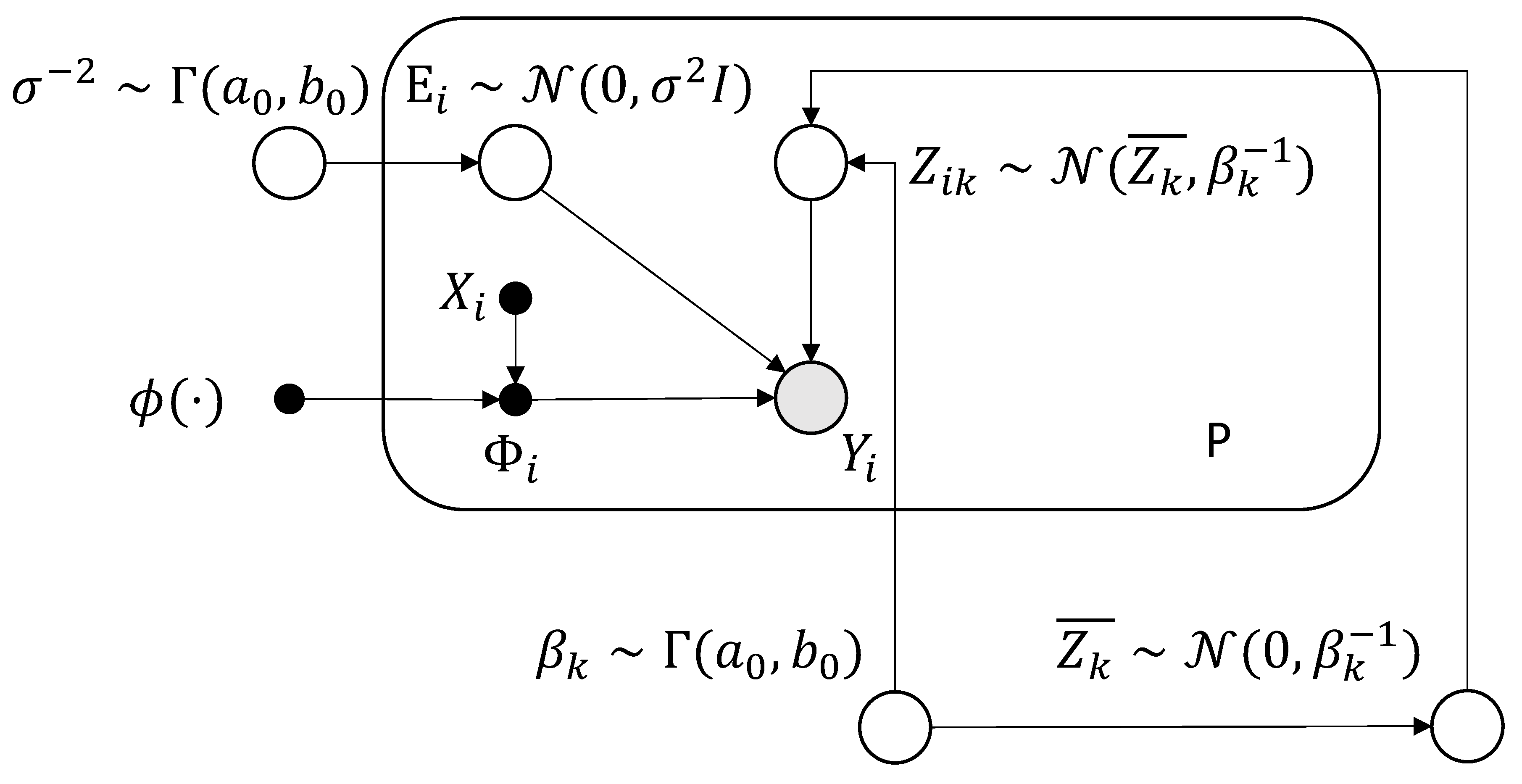
For effective model selection, we introduce a sparse prior over the coefficients of the basis functions. The sparse prior in the proposed model is based on automatic relevance detection (ARD) [62]. ARD evaluates the importance of a feature with a precision parameter estimated from the data. The model uses and for the numbers of components and basis functions, respectively, while signifies the overall magnitude of the mean coefficients:
In the model, are all variables of precision parameters, coming naturally with a conjugate prior of Gamma distribution. The probabilistic graphical model is depicted in Figure 1. Setting to a small value yields a vague Gamma prior that approximates a noninformative (Jeffreys-type) prior.
3. Methods
Based on the proposed formulation in Section 1.2, we estimate , the posterior of the unobserved values . This inference gives the point estimates of and the posterior predictive distribution of new data. For notational convenience, are omitted.
Using Bayes’ theorem, , but the exact posterior distribution is intractable because the evidence is intractable. Therefore, an approximate inference strategy is proposed. To facilitate this, we utilize variational inference (VI) [72], choosing a surrogate density from a parameterized family, denoted as , to approximate the posterior. Compared with classical methods like Markov chain Monte Carlo (MCMC) sampling, VI is typically faster per [72]. In our experiments, VI is about 85 times faster for the original Bayesian PCA formulation [45] as shown in Section 12.2 in the supplements.
3.1. Variational Bayesian Inference
Variational inference optimizes by maximizing the lower bound (minimizing the KL divergence between actual and surrogate distributions):
The mean-field variational family is used for . It simplifies the optimization by assuming the surrogate posterior distributions are independent, allowing each variable in the posterior to be optimized independently: . The posterior for each variable is chosen conjugate, further simplifying the optimization. Thus, the posteriors of the component scores Z, the weighting matrix W, and the mean weights are normal distributions. Here W is vectorized via without altering its normality assumption. Meanwhile, the posteriors of the precision variables of noise , components , basis functions , mean weights are Gamma distributions:
3.1.1. Update Steps
In mean field approximation using the surrogate posterior conditioned on observations Y, the lower bound is maximized with respect to each unknown . With the conjugate prior, the optimal updates (denoted with "←") make the moments of equal to the moments conditioned on the remaining parts of [72]:
From Equation (13), detailed update rules for each variable are presented subsequently, and the derivations of these formulas are in the supplementary material.
Updates for the parameters of the posterior for the precision of components :
where Equation (14) calculates the corrected degrees of freedom and Equation (15) calculates the corrected sum of squares. As and approach 0, the expectation of precision , which is , is exactly the inverse of the empirical or sample variance.
Updates for the parameters of the posterior of the precision of the mean weights :
Updates for the parameters of the posterior of the precision of basis functions :
Updates for the parameters of the posterior of the mean weights :
where denotes the diagonal matrix with diagonal entries given by . Equation (20) indicates that the eigenvectors of are solely determined by the sum of Gram matrices , while the eigenvalues of have a negative correlation with the scale of , the prior and data-dependent term . It is sensible because, for instance, large noise would result in large uncertainty in . In Equation (21), the data residuals, excluding component scores, are projected into the K-dimensional space through the inner product with and summed over all sample functions to calculate the mean weights.
Updates for the parameters of the posterior of the weights :
Equation (22) is similar to Equation (20), because it is correlated with , its prior and data-dependent terms and . In Equation (23), the data residual excluding the mean function is used to estimate the expectation of W.
Updates for the parameters of the posterior of the component scores :
where is a temporary variable denoting the Gram matrix of weighted kernel functions and denotes the covariance between and in .
Updates for the parameters of the posterior of the noise :
where H is a temporary variable that is updated by
Nearly noninformative (vagor) priors, i.e., with almost zero , introduce an inherent identifiability ambiguity in our formulation, specifically, in the product of the precision parameters and (Equations 20 and 22). In our model, scaling and by a specific factor while inversely scaling leaves the product (and hence the lower bound in Equation 5 ) unchanged. This inherent ambiguity can lead , , and to converge to extreme values, thereby challenging numerical stability during optimization. To mitigate this issue, we adopt a heuristic constraint to ensure that the smallest values of and remain within one order of magnitude of each other. Specifically, we enforce . If an update to any or would violate this constraint, that particular update is skipped while the rest of the parameters remain updated. This strategy does not alter the algorithm’s overall structure but stabilizes the optimization by curbing unnecessary flexibility in the precision parameters.
3.2. Scalable Update Strategy
The scalability of our algorithm so far is primarily challenged by the need to optimize the variational lower bound, over K basis functions. As indicated by Equation (22), time complexity is (or, alternatively, , typically dominated by the former), which becomes prohibitive when K is large. In practice, however, only a small subset of these basis functions is necessary for an accurate representation–those with non-negligible weights under our sparse prior.
To address this, we focus the updates on the subspace of active basis functions, denoted as , which comprises only those functions with non-negligible weights. The remaining basis functions, whose influence is minimal, are held fixed during optimization. Furthermore, the number of active principal components is noted as and set equal to , ensuring that the model spans the full range of possible ranks from 1 to . Consequently, we optimize using updates derived w.r.t. the objective -dimensional lower bound as an efficient surrogate of the full updates of w.r.t. the full lower bound , using only active basis functions. Meanwhile, the active dimensionality of the model is adjusted dynamically during optimization by activating or deactivating basis functions based on their precision parameters. For clarity, variables associated with the active subspace are annotated with the superscript (e.g., versus ).
3.2.1. Implicit Factorization
For notation clarity, we reorder the rows and columns of our parameter matrices to separate active components from inactive ones. Specifically, we partition as follows:
Here, the subscript A denotes variables belonging to the active subspace (i.e., those corresponding to basis functions), while and D denote the inactive components. Notably, the cross terms and involve both active and inactive components; these are updated implicitly, as proved in the supplements.
Following the strategy in [73], a basis function is deemed inactive if its precision exceeds a high threshold, i.e. and as . In the limit, the inactive basis functions decouple from the active ones, leading to the following mean-field factorization:
The factorization of and was already obtained in Equations (10) and (11). These factorizations allow us to decouple the update for the active subspace with the proof provided in the supplementary material.
It implies that only updates for are required as shown in Figure 2. This strategy reduces the computational complexity from to . Moreover, the active dimensions are initialized using a modified, multi-instance version of relevance vector machine [52], as detailed in Section 11 in the supplementary materials.
3.2.2. Low-Dimensional Lower Bound
This section shows how to optimize these active surrogates, e.g., , using updates of w.r.t. the -dimensional lower bound , which ultimately optimizes the full lower bound . To distinguish between the two, we denote the active surrogate posterior for the full model as and that for the reduced -dimensional model as . The active Gaussian surrogate posteriors are shared, e.g., . This implies updating is equivalent to updating , so we set the moments of the active distributions of the full model to match those of the reduced model. However, the surrogate posterior Gamma distributions differ between the two models. For example, the update of depends solely on , whereas also incorporates a cross term corresponding to the remaining dimensions. This difference is reflected in how the scale parameters depend on the number of active versus total basis functions, as shown in Equations (14), (16) and (18). Nonetheless, we prove that in the limit , the fixed point of the -dimensional updates of the complete surrogate equals that of the reduced surrogate . Consequently, the updates for , and are derived directly from the expectations of the reduced model :
These update Equations (34), (35), (36) prove to optimize in Theorem 1, 2 in the supplements.
3.2.3. Heuristic for Activating Basis Functions
The proposed method selects a relatively small set of basis functions from a potentially extensive set of possibilities. The computational costs are kept in check by recognizing that inactive basis functions do not interact with those active (with non-negligible weights). Due to computational constraints, we consider functions for activation sequentially rather than all at once. Thus, we propose Algorithm 1 to introduce unseen basis functions into the active set using a selective strategy akin to the heuristic approach described in [73].
The algorithm selects the top function, , from the inactive basis functions by gauging their correlation with residuals and applying an angle-based threshold relative to the subspace of . The correlation with residuals for is measured by . The angle-based threshold ensures a meaningful distinction from active functions. Next, the current active surrogate posterior is expanded by a dimension for , initiating optimization from the numerical maximum . Post optimization, the function gets retained if it falls below . Otherwise, the algorithm terminates. Efficiently, in trial optimization, the approach replaces one function with precision , if present.
| Algorithm 1 Search for new basis functions to activate |
|
4. Faster Variant
To enhance the computational efficiency of our primary algorithm, we introduce a faster variant, denoted as . This approach leverages conditional independence among the columns of W, enabling separate updates and thereby reducing computational complexity. Similar strategies have been described in [34,62]. The model is defined with an introduced variable for the coefficient noise as follows:
Similar to before, we assign a conjugate Gamma prior to the precision:
This formulation ensures that the columns of W are conditionally independent, allowing the variational distribution to factorize as: , thereby facilitating separate updates for each column. Consequently, the time complexity is reduced from to .
To align with the original model, it is necessary for and the associated variance parameters to approach zero. Having too high would allow the coefficient noise to corrupt the signal, biasing the model toward underestimating the true signal levels, particularly because this noise operates in the coefficient space where it introduces smooth, correlated variation (low entropy, like signals) that is harder to eliminate than high-frequency white noise (maximum entropy). Injecting the same amount of noise leads to an unbiased estimation of the signals but increases the estimation variance. Conversely, as decreases, the columns of W become dependent, violating the independence assumption inherent in variational inference. This dependency degrades the approximation quality and slows down the optimization process. Such dependency issues are well documented in both variational inference and MCMC literature–with recent efforts addressing them via structured VI [72] or blocked/collapsed Gibbs sampling [74]. Empirical validations of this noise impact are conducted with both in Section 5 and with Bayesian PCA [45,62] in Section 12.2 in the supplements.
To balance the trade-off between optimization speed and accuracy, we adopt a strategy of gradually decreasing the values of during the optimization iterations. Specifically, we initialize with a relatively large value and linearly decrease it from to over the first half of the iterations. After reaching , is fixed for the remaining iterations. This gradual reduction ensures that the algorithm initially maintains efficiency with benefits from minimizing interdependency among the columns of W to accelerate convergence while later preserving quality of the approximation by preventing the noise from obscuring signal components. We unify the scales by scaling the basis functions so that is standard normal and W is an identity matrix in initialization. Empirical evaluations indicate the strategy above is effective in most applications.
By implementing these modifications, offers a practical solution that substantially accelerates the algorithm without significant loss in accuracy, making it well-suited for large-scale, high-dimensional functional data analysis.
5. Results
The proposed method proves its effectiveness through simulations and applications to observed data sets.
5.1. Simulation Results
In simulations, we evaluate functional data analysis performance in model selection, estimated covariance accuracy, and extendability to multi-dimensional domains.
The model selection metric is the accuracy in estimating the number of principal components, which is the dimension of the compact subspace of signal variations. The configuration of the simulations in this section aligns with that established in [37], covering various scenarios. Simulated data sets derive from a latent generative model with variables with dimension r for the i-th sample function and noise corruption with a standard deviation of : where represent eigenfunctions, are the eigenvalues, signifies the mean function. Here, we consider five scenarios.
Scenario 1: Data generated with , , , , Here , i.e., the noise has a larger variance than the smallest signal.
Scenario 2: Similar to Scenario 1, but the third eigenfunction is replaced by a function with higher frequencies , and the principal component scores follow a skewed Gaussian mixture model. Specifically, the j-th component score has 1/3 probability of following a distribution, and 2/3 probability of following , for .
Scenario 3: Data generated with , , , ,
Scenario 4: Same as Scenario 3, but the component scores are generated from a Gaussian mixture model as Scenario 2.
Scenario 5: Data from , , , , , j-th component score obeying .
In each scenario, simulations produced 200 sample functions. We investigated 3 cases with sparse, medium, and dense sampling by assigning the number of observations per sample function . Each case in each scenario is repeated 200 times. The method’s performance was compared to fpca from [22], AIC and BIC in the 2022 release of pace [20], modified AIC and BIC in [37], and all the competing methods in [37]. For fpca, we set the candidate numbers of basis functions as [8,10,15,20], and the candidate dimensions of the process as [2,3,4,5] for Scenario 1-4 and [4,5,6,7,8] for Scenario 5. The other parameters are all set to the defaults. Due to its consistent overestimation of the true number of components–likely resulting from interference by correlated noise and less sparse precision priors–we excluded LFRM[34] from further comparisons (see Section 12.1.1 in the supplements).
Each estimation chose ten length-scales of functions, which are selected using cross-validation and k-means clustering. This adaptive strategy allows the algorithm to choose distinct length-scales at different locations of the definition domain, thereby accommodating varying smoothness characteristics inherent in complex functional data–a flexibility that is not possible when using a regular grid that forces a single length-scale across the entire domain [34]. Sparse sampling in Scenario 5 used five length-scales to avoid over-fitting. Figure 3 shows the length-scales and centers of the selected kernel basis functions for three different numbers of sample points, , in a random repetition of Scenario 5. The results reveal that the selected length-scales mainly concentrate around 0.07, with a few as high as 0.35–suggesting that the lower length-scales capture finer, high-frequency variations. The higher length-scales model the overall, lower-frequency quadratic mean structure and the constant baseline component. Furthermore, the estimated density functions of the selected length-scales exhibit consistent patterns across the three sampling densities, and the method selects 9, 11, and 12 basis functions respectively, demonstrating the algorithm’s adaptive fidelity and complexity based on the available observations. The supplements showcase the uncertainty evaluation in Figure 12.
Table 1, Table 2, Table 3, Table 4 and Table 5 show the results. Results for the first five methods are from [37]. Out of 15 cases, the proposed BSFDA exhibits the highest accuracy in 12. In the other 3 cases, the accuracy of BSFDA is comparable to the best result and is always above 0.950. demonstrates performance comparable to BSFDA when applied to medium-density and dense datasets with significantly higher efficiency which we detail in Figure 5 later. However, its efficacy diminishes with sparse data. This limitation arises because the parameter can bias model estimation in scenarios with insufficient data evidence, leading to an underestimation of signal variance. Consequently, tends to underestimate the number of components, particularly those capturing nuanced variations, in the presence of sparse observations. Nonetheless, with adequate data, achieves performance on par with the original model.
5.1.1. Mean Squared Error in Covariance Operator
The mean squared error across , a grid of 1000 index points:
where is the Frobenius norm, measure the accuracy of the estimated covariance. The quadratic measure of error with Frobenius norm for covariance estimators has been used by [75]. Methods compared include fpca of [22], pace of [20] with AIC and BIC, refund-sc of [21]. Only cases in scenario 5 were used because of the time constraints (e.g., refund-sc takes 6 hours for 20 repetitions with 50 points in scenario 5). As the most challenging, scenario 5 should provide the most compelling comparison. The results in Table 6 demonstrate that the proposed method is comparable to the best work in terms of estimated covariance accuracy. Specifically, dense sampling becomes prohibitive for refund-sc. The results highlight the benefit of continuous formulations, as seen in both fpca and the proposed method, over the grid-based optimization in conventional methods. again performed comparably well given data was adequate.
5.1.2. Multidimensional Functional Data Simulation
A simulation experiment with a four-dimensional index set reveals the proposed method’s advantages for high-dimensional data, where the gridding strategies of previous methods are impractical. The settings are as follows with a length-scale :
The observations include additive noise with a sigma of 4.472e-01. The cross-validation selects a length-scale of 0.405. The estimated noise sigma is 4.637e-01. The proposed method correctly estimates the number of principal components as 3 and selected 31 basis functions. As shown in Figure 4, the eigenfunctions are correctly estimated. In addition, the estimated mean function is zero, which is accurate.
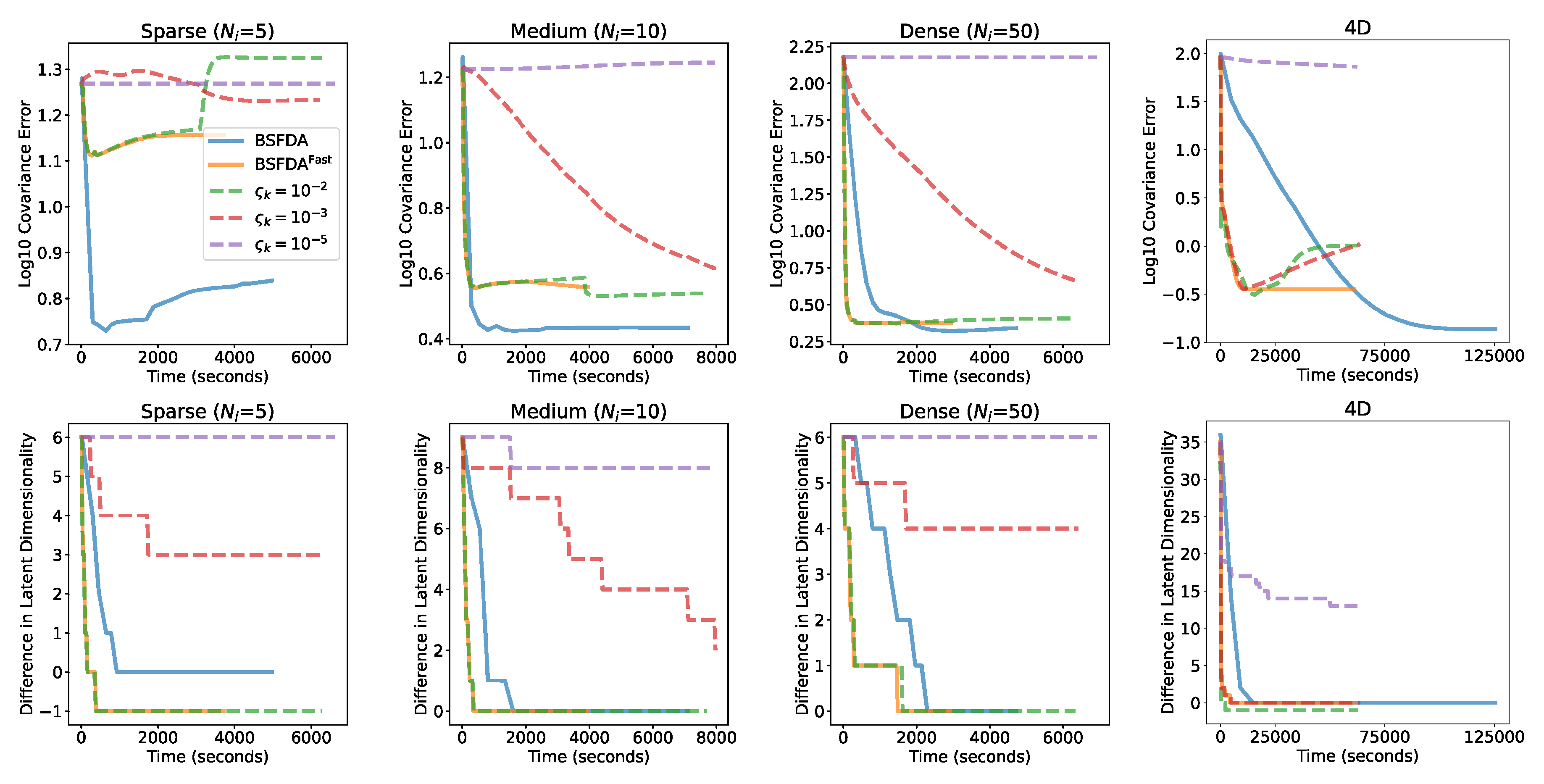
Next, we present a convergence comparison between BSFDA and under four different schedules for the coefficient noise . Specifically, we compare the default diminishing schedule from to with three fixed settings: , , and . We evaluate the covariance error and the discrepancy between the estimated/true dimensionality in one replicate of each sample density in Scenario 5, and the 4D simulation. For the 4D, we adopt a default initial of . As illustrated in Figure 5, achieves comparable accuracy to BSFDA while converging significantly faster than BSFDA in terms of both covariance errors and component estimation for medium and densely sampled data. In the 4D case, converges in covariance estimation after approximately 10,000 seconds and in dimensionality after around 4,000 seconds, compared to roughly 100,000 seconds and 13,000 seconds, respectively, for BSFDA. However, for sparse data, exhibits reduced estimation accuracy and underestimates the number of components by one. A similar decline in accuracy is observed in the 4D simulation when data sparsity is high. This limitation arises because the introduction of coefficient noise biases the model towards eliminating signals that are deemed insignificant. Moreover, when comparing the three fixed- variants of the fast algorithm, a clear trade-off emerges: smaller reduce overall error but slow down the optimization due to increased dependency among variables. These results collectively demonstrate the effectiveness of our chosen schedule in , as it balances both efficiency and accuracy.
Figure 5.
Convergence plots for Scenario 5 in Yehua and the 4D simulation. The upper row displays the covariance error against time, while the lower row illustrates the difference between the estimated and true number of components.
Figure 5.
Convergence plots for Scenario 5 in Yehua and the 4D simulation. The upper row displays the covariance error against time, while the lower row illustrates the difference between the estimated and true number of components.
5.2. Results on Public Data Sets
The proposed method’s practicality was validated with 2 application data sets, CD4 and wind speed measurements.
5.2.1. CD4
CD4 data, a classical form of functional data, received attention in [1,20,22]. CD4 cell counts gauge the immune system’s response to human immunodeficiency virus (HIV) infection, which leads to a progressive reduction in CD4 cell counts. The Multicenter AIDS Cohort Study (MACS) [76] provided the CD4 data. This dataset consists of CD4 percentages from 283 male human subjects that were HIV positive, each with 1 to 14 repeated measurements over time in years. Subjects were scheduled for reevaluation at least semiannually. However, missed visits caused a sparse and uneven distribution of measurements. The proposed method used five length-scales selected from cross-validation and k-means clustering. Finally, the model selected 9 basis functions. Figure 6 displays the estimated mean function, eigenfunctions, and curves of the observations. The mean function reflects the overall decreasing tendency with the progression of the disease. The eigenfunctions are obtained by applying singular value decomposition of the covariance operator that is discretized (for visualization purposes only) with a grid of 50 evenly spaced points over the whole timeline. The first eigenfunction is relatively flat and mainly captures the subject-specific average magnitude of the CD4 counts, consistent with the finding of [1,20,22]. The second eigenfunction captures the simple linear trend of the variations, as described in [22]. The third eigenfunction captures the piece-wise linear time trend with a breakpoint near 2.5 years since baseline. [1,20] found similar eigenfunctions.
5.2.2. Wind Speed
Wind-speed data, collected from 110 locations across Utah’s Salt Lake Valley, varies between 11 to 1440 measurements. The proposed method leverages ten length-scales selected from cross-validation and k-means clustering. Figure 7 illustrates the estimated mean function, curves of the observations, eigenfunctions, and covariance. The horizontal axis represents the seconds starting from 12:00 AM Greenwich Mean Time (GMT) on June 15, 2023, which corresponds to 6:00 PM in Salt Lake City. In Figure 7a, the estimated mean function depicts two pronounced peaks observed approximately at 8:00 PM and 6:00 AM, as well as two troughs around 12:00 AM and 12:00 PM. This pattern aligns with the diurnal cycle, particularly highlighting the thermal activities associated with sunset and sunrise. The peaks during sunset and sunrise are due to the interplay of topographical features, which result in specific breezes, such as the land breeze near the Great Salt Lake and the distinct mountain and valley breezes. The troughs, on the other hand, reflect moments when the atmosphere is at its most stable, with minimal thermal activities disrupting wind patterns. The complexity of the data is distilled and represented using 12 descriptors with 17 basis functions. As Figure 7b shows, the primary eigenfunction is relatively level, indicating that the most significant variation is the location-specific average magnitude. Its profile echoes the influence of sunrise and sunset observed in the mean function, with elevations around 7:00 PM and 5:00 AM and subdued patterns during other times, indicative of a similar atmospheric stability. The estimated covariance in Figure 7c highlights variance peaks around 8 PM and 5 AM, as well as a strong correlation between these periods. This underscores the effects of location-specific topographic factors on wind speed.
5.2.3. Modeling Large-Scale, Dynamic, Geospatial Data
Here, we demonstrate the scalability on both the size of the measurements and the dimensionality of our framework. For this, we apply it to the ARGO dataset, which consists of ocean temperature measurements from more than 4,000 locations, at multiple depths, and time points [71]. ARGO is a nearly global observing system for ocean temperature, salinity, and other key variables via autonomous profiling floats. As of 2019, ARGO has generated over 338 gigabytes of data from 15,231 floats [71]. We focused on high-quality ("research" mode option in the database API) data from 1998 to 2024 for depths between 0–200 meters in the open-access snapshot of Argo GDAC of November 9, 2024 [77]. The number of measurement points per year varies widely–from 38,931 up to over 11 million, with 127 million in total. Figure 8 illustrates a global map of sea surface temperature measurements from February 2021, highlighting the dataset’s extensive spatial coverage.
In our modeling, each year’s data is treated as a single underlying function of four variables: latitude, longitude (on the spherical Earth), depth, and intra-annual time (modeled as a periodic variable). Note that the spatial data lies on a sphere and the time is a circle, assuming the periodicity of the time of the year. Our approach models these measurements holistically–without resorting to moving windows or sub-modeling–thereby preserving the continuous nature of the data and enabling the extraction of meaningful global, seasonal, and depth-dependent trends. Furthermore, the unique geospatial and temporal structure of Argo data, with spatial coordinates on a sphere and time exhibiting periodicity, necessitates specialized modeling techniques. Given that our model is 4 dimensional, the 4D kernel is defined as a product of the following kernels, following the design strategy for climatological data in [19]. The geospatial kernel on the sphere is a radial basis function (RBF) on geodesic distances. To ensure periodicity, the temporal kernel is an Exp-Sine-Squared where is the length-scale. For depth, we use a Gaussian kernel.
The numeric data (excluding metadata) as input to the model was approximately 4 GB. For length-scale selection, we used Gaussian process regression on a small subset of 2,000 randomly selected data in 2016 (medium size of measurements) for a cross validated RMSE which we optimize with a grid search. The specific length scales were set as follows: geodesic length scale of km, depth length scale of 70 m, time length scale of 3, and periodicity of 1. For evaluation, we held out 10% of the depth profiles (a single round trip of a buoy from surface to a depth at the same coordinate) from each year as testing data, following [78]. The total training set contained roughly 114 million points. Because the sample spacing is typically small relative to the selected length-scales, we apply agglomerative clustering to 10,000 randomly chosen index points, reducing them to 2,000 candidate basis functions. These candidate basis functions–precomputed for efficiency–took roughly 1.7 TB of memory. Computations were performed with 24 threads on a server equipped with 192 Intel® Xeon® Platinum 8360H CPUs @ 3.00GHz and 3TB RAM. Initialization was conducted using the modified RVM for 200 iterations for initial basis functions, using a stochastic optimization with a 1,000-batch size per year. Then executed for 10,000 iterations, where the heuristic to include new bases also used a 1,000-batch size per year. With these computational strategies and heuristics, the entire modeling process was completed in 15 hours.
The proposed approach selected 163 effective basis functions and condensed them into 16 principle components. The final model occupies merely 50 MB of storage. The interpolation yielded a root mean square error (RMSE) of 1.95 and an of 94.2% on testing data, reflecting a reasonable balance between global dimension reduction and fidelity. The estimated white noise level was also 1.95, indicating that the training data adequately covers the underlying variability in the ARGO observations, and the final model is reasonably generalizable.
Figure 9 presents 2D visualizations of geospatial interpolations at three depths (in decibars, roughly meters) and a specific time (May 29, 2021) around 1°S and 30°W, each with three views. We have picked one measurement as the central point, denoted as the red circle, and selected a narrow window (±1 decibar, ±1 day) around this center. The cyan and fuchsia circles represent training and testing data, respectively, within this window. Their sizes indicate distance along the unplotted dimensions (depth and time here), reflecting variations in these dimensions. The visualizations show that temperatures are warmer near the equator and decrease with depth. The match between interpolated values and actual measurements demonstrates consistency in capturing broad spatial and vertical variations.
Figure 10 complements this by illustrating interpolation in the depth-time slices while holding the geospatial coordinates fixed, focusing on mixed layer characteristics. The "mixed layer" refers to a region of nearly uniform temperature, which is crucial for understanding thermodynamic potential and nutrient cycling [79]. Here, the plot uses a window of 50 km to include actual measurement, and the circle sizes denote geodesic distance from the chosen center. We plot every fifth measurement vertically to reduce overlap and improve clarity. Figure 10a uses the same center point, 1°S and 30°W, as in Figure 9, exhibiting a shallow mixed layer with pronounced vertical gradients. In contrast, Figure 10b adopts a center at a higher latitude, 49°N and 29°W, where the model reveals a deeper mixed layer. The temperature there remains relatively stable below the surface. The dominant variations are cyclic seasonal changes, which are warmer near the surface around September. As is shown, the vertical sequence of the center and the nearby testing sequence match the interpolation closely. These results confirm that the mid-latitudes exhibit a stronger seasonal cycle [79], and that accurately approximates the actual measurements.
To our knowledge, this is the first time the ARGO dataset has been modeled in a full 4-dimensional principal component model, with the correct domain topology. We incorporate the entire period of 27 years rather than shorter spans (e.g., 2004-2008 or 2007-2016) [78,80,81]. Instead of segmenting the dataset into localized spatiotemporal windows, we process the entire 4D domain (latitude, longitude, depth, and intra-annual time) in a single holistic framework. Previous studies were typically tailored for ARGO datasets and handled each depth, month, or spatial region separately, restricting correlation estimates to limited windows (e.g., 1000 km and three months) while excluding data with large offsets [78,81]. In addition, they require repeated on-demand model fitting that can hinder scalability. Our kernel-based framework, by contrast, is broadly applicable to general functional data, only requiring kernel definitions for the domain. Although global dimension-reduction inevitably introduces some residual noise, the kernel-based design is extensible to finer spacing or multiple length scales if higher precision is needed. Furthermore, inference with our model is simply the evaluation of the active 163 active basis functions weighted by the 16 principal components. Interpolation over a 300×300 grid only takes about two seconds. By contrast, previous methods with Gaussian process regression require a weighted sum of all the measured data within a certain window. The parametric representations also facilitate straightforward derivative and integration calculations, which are essential for investigating ocean temperature stratification and heat content [78]. In summary, the Argo dataset provides an ideal testbed for our method, as it captures the dynamic behavior of high-dimensional geospatial data in a continuous framework. A more comprehensive study of ARGO is beyond this paper’s scope. Nonetheless, the results here confirm the clear advantages of the proposed method for large-scale, high-dimensional functional data.
6. Discussion
This paper proposed BSFDA, a novel framework for functional data analysis with irregular sampling, integrating model selection and scalability in one unique, coherent, and effective algorithm. Our extensive empirical studies, including both simulations and real world applications, show that BSFDA offer superior covariance estimation accuracy with remarkable efficiency.
In terms of accuracy, our method excels in model selection, consistently achieving top-tier performance. The accuracy of the covariance operator estimation also rivals that of the best existing methodologies in the field. This shows that our approach can not only handle large and complex datasets, but also ensures high accuracy and precision in the results it produces. Our method’s superiority compared to existing techniques is expected owing to the inherent iterative nature of data smoothing and covariance estimation in our approach.
In terms of scalability, our method demonstrates a linear growth of time complexity with the size of the dataset, and impressively, the computations are executed in a small, -dimensional subspace. This ensures that as the datasets grow larger and more complex, the performance of our model remains robust and efficient. Additionally, we introduced a faster variant, , which performs similarly to BSFDA on medium and dense datasets with significantly reduced computational cost. This leap in efficiency enabled a full 4-dimensional functional modeling, for the first time, of the large scale oceanic temperature dataset across 27 years (ARGO) [71]. Although can underestimate signal strength under very sparse sampling, the vanilla BSFDA effectively complements and alleviates this issue.
Looking ahead, it would be interesting to explore how extensions of regular PCA, such as simplified PCA and robust PCA [42], can be integrated within our proposed framework. These extensions will enhance the flexibility and robustness of our method, further improving its adaptability to various data conditions. In addition, we see potential in examining the extensions of functional PCA, such as time warping, dynamics, and manifold learning [1]. In particular, shape analysis emerges as a direct application of time warping. Such extensions would push the boundaries of what our proposed method could achieve, potentially enabling it to handle an even wider array of data structures and complexities.
In conclusion, our research findings affirm the proposed framework’s effectiveness and adaptability in advanced functional data analysis. Nonetheless, the method’s potential remains broad, and future work promises to widen its scope and refine its performance. By unifying sparse Bayesian learning, kernel-based expansions, and efficient variational inference, BSFDA offers a powerful foundation for large-scale, high-dimensional FDA challenges.
7. System of Notation
Table 7 summarizes the notation used in Section 1.2 and Section 3.2.3, providing a reference for the derivations. All vectors in the table are represented as row vectors.

Table 7.
Symbol definitions in formulation.
| Symbol | Meaning |
| The i-th sample function | |
| One M-dimension index | |
| M | Dimension of the index set |
| K | Number of all basis functions |
| J | Number of all components |
| P | Number of sample functions |
| Number of measurements of the i-th sample function | |
| Index set of the i-th sample function | |
| Measurement of the i-th sample function | |
| Component scores of the i-th sample function | |
| Coefficients of basis functions in the mean function | |
| Measurement errors of the i-th sample function | |
| Weighing matrix of basis functions in the eigenfunctions | |
| The j-th row and k-th column of W | |
| The kernel function | |
| The scale parameter of (j-th component) | |
| The scale parameter of (k-th basis function) | |
| The standard deviation of measurement errors | |
| The communal scale parameter of | |
| The union of all the centered kernel functions | |
| Value of centered kernel function at | |
| Coefficients of the i-th sample function | |
| Coefficient noise of the i-th sample function | |
| The scale parameter of k-th coefficient noise |
Table 8 summarizes the notation used in Section 2.2.
Table 8.
Notation used in formulating the optimization.
| Symbol | Meaning |
| All the latent variables. | |
| The surrogate posterior distribution of variable · | |
| The joint surrogate posterior distribution of all variables except · | |
| The mean and covariance of · in , e.g. | |
| The shape and rate parameters of , e.g. | |
| The expectation of variable · over density | |
| The lower bound of surrogate posterior with K basis functions | |
| Gram matrix of the kernel functions for the i-th sample function, | |
| Number of active/effective basis functions | |
| Number of active/effective components | |
| Log likelihood of in multi-sample relevance vector machine | |
| Covariance of in multi-sample relevance vector machine | |
| Posterior covariance of in multi-sample relevance vector machine | |
| Log likelihood of in multi-sample relevance vector machine | |
| The infinitesimal number | |
| Threshold/tolerance of · |
8. Variational Update Formulae
For brevity, the joint posterior is shown with the vague Gamma prior parameters , , and the observation index X omitted:
Derivation of Equations (14) and (15):
According to Equation (13) and the posterior in Equation (50), the update formulae for the surrogate distribution is:
where we have omitted terms that is conditionally independent of. By definition
By equating Equations (51) and (52), the updates for are
Derivation of Equations (14) and (15):
According to Equation (13) and the posterior Equation (50), the update formulae for is:
where we have omitted terms is conditionally independent of. By definition
By equating Equations (55) and (56), the updates for are
Derivation of Equations (18) and (19):
According to Equation (13) and the posterior Equation (50), the update formulae for is:
where we have omitted terms that in conditionally independent of. By definition
By equating Equations (59) and (60), the updates for are
Derivation of Equations (20), (21):
According to Equations (13) and the posterior Equation (50), the update formulae for is:
where we have omitted terms that is conditionally independent of. By definition
By equating Equations (63) and (64), the updates for are
Derivation of Equations (22), (23):
According to Equation (13) and the posterior Equation (50), the update formulae for is:
where we have omitted terms that W is conditionally independent of. By definition
By equating Equations (67) and (68), the updates for are
Derivation of Equations (24), (25) and (26):
According to Equation (13) and the posterior Equation (50), the update formulae for is:
where we have omitted terms that is conditionally independent of. By definition
By equating Equations (70) and (71), the updates for are
According to Equation (13) and the posterior Equation (50), the update formulae for is:
where we have omitted terms that is conditionally independent of. By definition
By equating Equations (74) and (75), the updates for are
9. Scalable Update for BSFDA
9.1. Implicit Factorization
We initialize the inactive precision parameters as:
Under these settings and subsequent variational updates (using Equations (78) and (79)), in the limit as , the surrogate distributions satisfy:
For convenience, we initialize with the above properties.
Lemma 1.
If and , then the variational distribution over W factorizes as in the limit as .
Proof.
We express the distribution as
The factorization holds if the off-diagonal block matrices in , e.g. , are all zero, i.e., the blocks are mutually independent. Initially, this is ensured by the definition for the initial status in Equation (82). Thus, we only need to show the statement remains true after is updated, i.e., after Equation (22) is applied with the inactive scale parameters and fixed at . First we regard , i.e., the covariance of the union of after vectorization, as one block. By the block matrix inversion formula, we get and consequently . Next, apply block matrix inversion formula to in Equation (22) and we get , yielding the desired factorization. □
Lemma 2.
If , then the implicit factorization holds in the limit as .
Proof.
It is similar to the proof for Lemma A1. Because , we only need the off-diagonal block is zero, i.e., . Initially, it is ensured by definition for the initial status in Equation (81). is updated by Equation (20), Applying block matrix inversion formula with the inactive , we get , establishing the factorization. □
Lemma 3.
If or , then in the limit as .
Proof.
For initial status, apparently the largest is . Because either or , after updates from Equations (22) and (23) are applied, by Woodbury matrix identity. □
Lemma 4.
If , then the implicit factorization holds in the limit as .
Proof.
It is similar to the proof for Lemma 1. Because , only is needed. Initially, it is ensured by definition for the initial status Equation (80). is updated by Equations (24) and (25). In Equation (24), when or , applying Lemma 3. Applying block matrix inversion formula to Equation (25), , , thus proving the implicit factorization □
9.2. Scale Parameters
Here we state the theorems that justify we can use updating rules for based on to update (and similarly, for , for ) and it does maximize ultimately.
Lemma 5.
, i.e., either or , after updating and by Equations (22) and (23), .
Proof.
According to Equations (78) and (79), if or , either or respectively.
In the limit as , using Equation (22) and block matrix inversion formula we get
In the limit as and using Equation (23)
Equation (84) uses the fact that elements in are all based on block matrix inversion formula. Thus,
□
Lemma 6.
, after updating by Equations (20) and (21), .
Proof.
If , .
Then using Equation (20) and block matrix inversion formula we get
Using Equation (21)
Equation (87) uses the fact that elements in are all .
□
Theorem 1.
, updates of and will converge at given , and conditions in Equations (80)-(79) are satisfied in the limit as .
Proof.
The updates for derived from are
It involves and therefore they need to be kepted updated. Apply Theorem 5 for Equation (91) and we can get
Applying Equation (92) in an iterative manner, we will get a sequence of updates for . Solving
Thus, we can get that the sequence will converge at
As a result, . □
Theorem 2.
, updates of and will converge at given , and conditions in Equations (80)-(79) are satisfied in the limit as .
Proof.
The updates for derived from is
It involves and therefore they need to be kepted updated. Apply Theorem 5 for Equation (98) and we can get
Applying Equation (99) in an iterative manner, we will get a sequence of . Solving
Thus, we can get that the sequence will converge at
As a result, . □
Theorem 3.
Updates of and will converge at given , and conditions in Equations (80)-(79) are satisfied in the limit as .
Proof.
The updates for derived from is
It involves and therefore they need to be kept updated. Apply Lemma 6 for Equation (106) and we can get
Applying Equation (108) in an iterative manner, we will get a sequence of updates for . Solving
Thus, we can get that the sequence will converge at
As a result, . □
In practice, due to limitations in numerical representation, we restrict values so that the active precision parameter estimates would not really go to infinity:
9.3. Weights and Noise
Here is how to update in a scalable manner, using computation in the dimension subspace only.
Theorem 4.
and share the same update rule for , i.e.,
Proof.
Apply Lemma 3 to Equation (24) we get
Apply block matrix inversion formula to Equation (25) we get
Apply block matrix multiplication and Theorem 5 to Equation (26) conditioned on Equation (81) we get
□
Theorem 5.
and share the same update rule for , i.e.,
Proof.
Apply block matrix inversion formula to Equation (20) conditioned on and we get
Apply block matrix multiplication and Theorem 5 to Equation (21) conditioned on Equation (80) we get
□
Theorem 6.
and share the same update rule for , i.e.,
Proof.
Apply block matrix inversion formula to Equation (22) conditioned on and , we get
Apply block matrix multiplication and Theorem 5 to Equation (23) conditioned on Equation (80) and Equation (81), we get
□
Theorem 7.
and share the same update rule for σ, i.e.,
where
Proof.
Apply block matrix multiplication and Theorem 5 to Equation (28) conditioned on Equations (80) and (81), we get
□
We show share the same update formulas as those derived from the low-dimensional lower bound: . Thus, in practice, if suffices to update ; we can then increase by including new basis functions. This process proves to implicitly maximizes with .
9.4. Low-Dimensional Lower Bound
We now have updating formulas for the parameters in the active subspace. is updated by Equations (114), (115) and (116). is updated by Equations (124) and (125). is updated by Equations (120) and (121). are updated by Theorem 1, 2 and 3, with the companion of implicit updates of . is updated by Equations (130), (128) and (129). All the updating rules are identical to those derived from the low-dimensional lower bound with basis functions. Therefore, in practice all we need is to optimize , with time complexity of , as described in Theorem 8, and then check if a new basis function should be included in the model.
For numerical stability, we scale such that at the beginning of Algorithm 2.
Theorem 8.
The lower bound can be optimized using Algorithm 2 with time complexity of .
Proof.
It is a consequence of Theorems 1, 2, 3, 4, 5, 6, 7. □
| Algorithm 2 Variational inference |
|
10. Scalable Update for BSFDAFast
For brevity, we denote the covariance of as S, i.e., . S is diagonal and . The variational update formulas are as follows:
Notably, the columns of W becomes conditionally independent with the introduction of the slack variable , akin to the strategy described in [34,62]. Then the surrogate posterior of W factorizes over the columns, thereby requiring calculating the covariance of each column separately instead of the entire W at once. Thus, the computational complexity is significantly reduced. This factorization is introduced on top of the existing factorizations, thus the low-dimensional optimization strategy of BSFDA also applies to .
11. Fast Initialization
In order to efficiently obtain a good initialization for the unknowns to be estimated, e.g. , and , we approximate the model so that we can adopt a fast strategy maximizing marginal likelihood using direct differentiation that is similar to [73]. This initial serves to select the basis functions to start with.
We introduce for easier marginalization:
The approximated probabilistic graphical model is shown in Figure 11.
Figure 11.
Probabilistic graphical model for the simplified model.
11.1. Maximum Likelihood Estimation
We apply maximum likelihood estimation for point estimates of .
where . Conditioned on these estimates, we can calculate the expectation of Z.
Optimization of
We set the differentiation to zero, i.e., , and get:
where
We differentiate with respect to and zero the derivative, i.e., , to get:
We approximate Equation (158) by and . This way we can apply the update with only the active basis functions.
Optimization of :
We use EM to optimize . In E step:
where .
In M step
The optimization iterates between the E-step Equations (159) and (160), and the M-step Equation (161).
In practice, we need only , and they can be calculated using the active basis functions. Thus, similar to [73], all the computations can be operated with only the active basis functions and thus it computationally efficient. This is described in Algorithm 3.
| Algorithm 3 Multi-sample relevance vector machine |
|
We apply Sylvester’s determinant theorem to Equation (157) and get
We apply Woodbury matrix identity to Equation (157) and get
We first expand
where we plug in Equations (165) and (166) and define in a similar way to [73]. The sparsity factor can be seen to be a measure of the extent that the basis function overlaps those already present in the model under the measurements at index set . The quality factor is a measure of the alignment with the error of the model at with that basis function excluded. Because we are representing the mean functions using only the active basis functions, i.e., when , Equation (154) only uses the K active basis functions. Similarly, Equation (155) only uses the K active basis functions.
11.2. Optimization of β,Z ¯
Derivation of Equation (152):
We differentiate with respect to
We further adopt the approximation . Because is a discrete measure of the overlapping between the basis functions, it should remain invariant with respect to different sampling grid given the number of measurements is adequate and similar. Alternatively, the Expectation maximization scheme can also be applied and is guaranteed to increase the likelihood in each iteration until convergence. However, we opt for this gradient descent with approximations for its advantage in speed to obtain a reasonable initialization. This way we set the approximated differentiation to zero
Because is a scale parameter, we need . Consequently, the optimal value for to maximize dependents on the sign of . When , the maximum of is achieved at .
On the other hand when , is monotonically increasing with respect to and therefore we should have in order to maximize .
More intuitively, Equation (174) can be regarded as a weighted summation of the estimation of using each individual sample function and it automatically assigns more weights to those with more measurements. Therefore, this optimization strategy is supposed to provide reasonable estimates even when the sampled functions have different numbers of measurements.
Derivation of Equation (158):
We differentiate with respect to and zero the derivative to get
11.3. Optimization of σ
Derivation of Equations (159) and (160):
We use the Expectation maximization strategy with latent variables . It is similar to that used in [52]. It introduces a surrogate function, the log likelihood for the complete data , that is easier to optimize and in theory the process ultimately maximizes .
For the E-step, we calculate the posterior of .
Therefore,
where
Derivation of Equation (161):
In M-step, we need to maximum conditioned on with respect to ,
We differentiate with respect to and set to 0
12. Experiments
12.1. Benchmark Simulation
Figure 12 presents the application of the proposed BSFDA to the simulation benchmark (Scenario 1) outlined in [37]. While prior analyses have utilized this benchmark, the current experimental configuration is specifically adapted to highlight the method’s capacity for uncertainty quantification. The experimental design consists of 20 functional observations, each sampled at either 3 points (with a 20% probability) or 10 points (with an 80% probability), determined via random assignment. The number of sampled functions is decreased from 200 to 20 to underscore the effect and estimation of uncertainties. The actual white noise standard deviation is 0.4472, while the estimated standard deviation is 0.4839. The component number is also correctly estimated as 3. The figure depicts the true underlying function, the discrete observational data, and the corresponding functional estimates, accompanied by their respective 95% truncated uncertainty intervals.
Notably, the uncertainty associated with sparsely sampled functions exhibits substantial inflation in regions devoid of observations. In contrast, in sampled regions, the uncertainty aligns closely with that of densely sampled functions, approximating twice the standard deviation of the white noise. Additionally, the uncertainty bounds for the estimated mean function are presented, demonstrating reduced variability relative to individual function estimates.
Figure 12.
Application of the proposed BSFDA to the simulation benchmark from [37], illustrating the true mean function (blue), observed measurements from two functions sampled at different densities (light blue for sparse, orange for dense), and the corresponding functional estimates with 95% truncated uncertainty intervals.
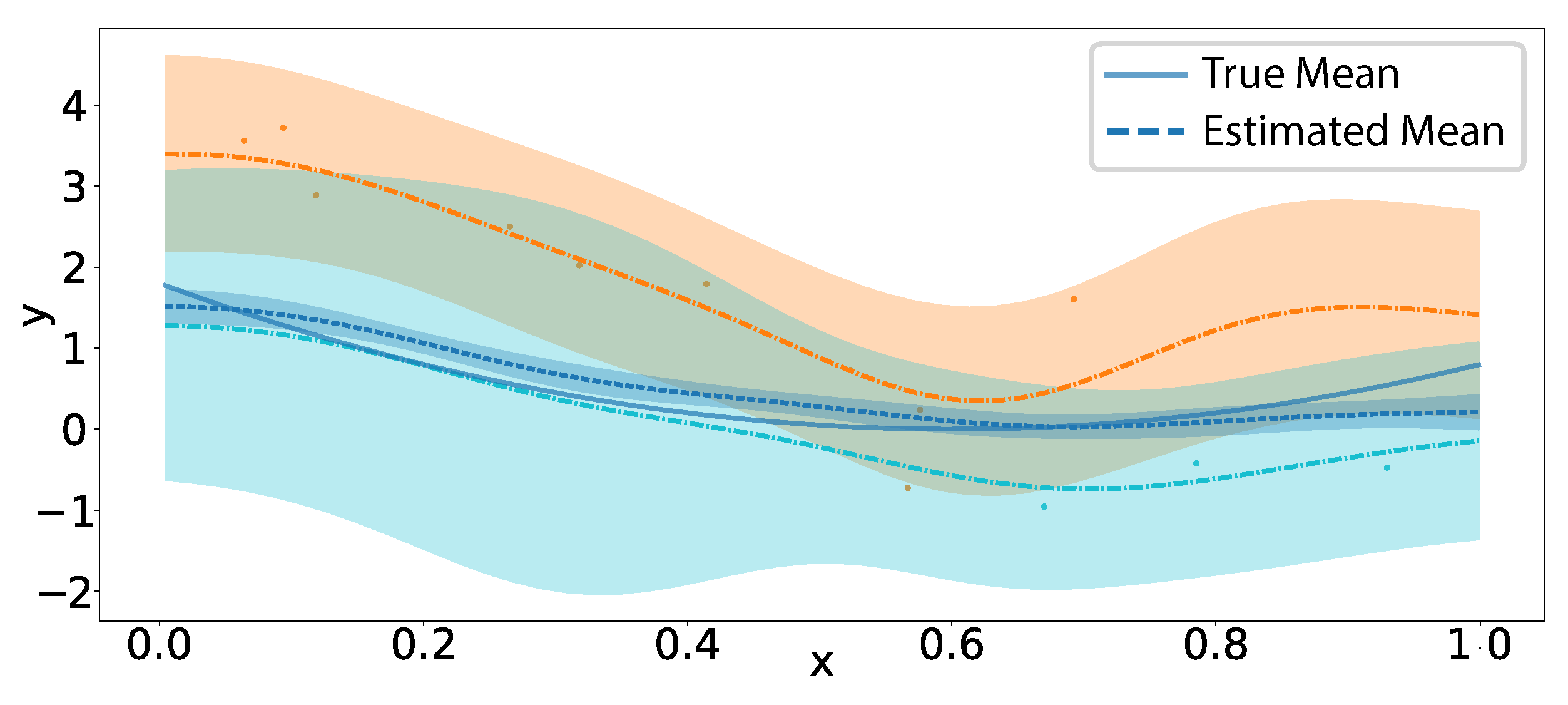
Table 9.
Distributions of the estimated component number for Scenario 1 (r=3).
| AIC | BIC | fpca | BSFDA | ||||||||
| 5 | 0.000 | 0.000 | 0.155 | 0.005 | 0.000 | 0.000 | 0.000 | 0.000 | 0.000 | 0.000 | |
| =2 | 0.008 | 0.405 | 0.335 | 0.565 | 0.215 | 0.000 | 0.000 | 0.000 | 0.000 | 0.985 | |
| =3 | 0.000 | 0.580 | 0.380 | 0.410 | 0.735 | 0.650 | 0.880 | 0.645 | 0.995 | 0.015 | |
| =4 | 0.121 | 0.010 | 0.115 | 0.010 | 0.045 | 0.335 | 0.120 | 0.235 | 0.005 | 0.000 | |
| 0.870 | 0.005 | 0.015 | 0.010 | 0.005 | 0.015 | 0.000 | 0.120 | 0.000 | 0.000 | ||
| 10 | 0.000 | 0.000 | 0.000 | 0.000 | 0.000 | 0.000 | 0.000 | 0.000 | 0.000 | 0.000 | |
| =2 | 0.000 | 0.005 | 0.040 | 0.040 | 0.005 | 0.000 | 0.000 | 0.000 | 0.000 | 0.075 | |
| =3 | 0.000 | 0.980 | 0.670 | 0.955 | 0.985 | 0.880 | 0.920 | 0.645 | 1.000 | 0.910 | |
| =4 | 0.000 | 0.015 | 0.255 | 0.000 | 0.010 | 0.120 | 0.080 | 0.235 | 0.000 | 0.015 | |
| 1.000 | 0.000 | 0.035 | 0.005 | 0.000 | 0.000 | 0.000 | 0.120 | 0.000 | 0.000 | ||
| 50 | 0.000 | 0.000 | 0.000 | 0.000 | 0.000 | 0.000 | 0.000 | 0.000 | 0.000 | 0.000 | |
| =2 | 0.000 | 0.000 | 0.000 | 0.000 | 0.000 | 0.000 | 0.000 | 0.000 | 0.000 | 0.000 | |
| =3 | 0.000 | 1.000 | 0.830 | 1.000 | 1.000 | 1.000 | 1.000 | 0.890 | 0.980 | 0.945 | |
| =4 | 0.000 | 0.000 | 0.150 | 0.000 | 0.000 | 0.000 | 0.000 | 0.060 | 0.020 | 0.050 | |
| 1.000 | 0.000 | 0.020 | 0.000 | 0.000 | 0.000 | 0.000 | 0.050 | 0.000 | 0.005 |
Table 10.
Distributions of the estimated component number for Scenario 2 (r=3).
| AIC | BIC | fpca | BSFDA | ||||||||
| 5 | 0.000 | 0.000 | 0.230 | 0.000 | 0.000 | 0.000 | 0.000 | 0.000 | 0.000 | 0.000 | |
| =2 | 0.000 | 0.205 | 0.395 | 0.000 | 0.140 | 0.050 | 0.075 | 0.000 | 0.000 | 0.960 | |
| =3 | 0.005 | 0.630 | 0.245 | 0.375 | 0.605 | 0.570 | 0.620 | 0.475 | 1.000 | 0.040 | |
| =4 | 0.125 | 0.155 | 0.110 | 0.440 | 0.210 | 0.345 | 0.275 | 0.350 | 0.000 | 0.000 | |
| 0.870 | 0.010 | 0.020 | 0.185 | 0.045 | 0.035 | 0.030 | 0.175 | 0.000 | 0.000 | ||
| 10 | 0.000 | 0.000 | 0.000 | 0.000 | 0.000 | 0.000 | 0.000 | 0.000 | 0.000 | 0.000 | |
| =2 | 0.000 | 0.000 | 0.170 | 0.000 | 0.000 | 0.000 | 0.000 | 0.000 | 0.000 | 0.000 | |
| =3 | 0.000 | 0.710 | 0.665 | 0.570 | 0.805 | 0.825 | 0.850 | 0.640 | 1.000 | 0.995 | |
| =4 | 0.005 | 0.260 | 0.135 | 0.355 | 0.185 | 0.175 | 0.150 | 0.235 | 0.000 | 0.005 | |
| 0.995 | 0.030 | 0.030 | 0.075 | 0.010 | 0.000 | 0.000 | 0.125 | 0.000 | 0.000 | ||
| 50 | 0.000 | 0.000 | 0.000 | 0.000 | 0.000 | 0.000 | 0.000 | 0.000 | 0.000 | 0.000 | |
| =2 | 0.000 | 0.000 | 0.000 | 0.000 | 0.000 | 0.000 | 0.000 | 0.000 | 0.000 | 0.000 | |
| =3 | 0.000 | 0.630 | 0.795 | 0.955 | 0.945 | 1.000 | 1.000 | 0.950 | 1.000 | 0.950 | |
| =4 | 0.000 | 0.320 | 0.185 | 0.045 | 0.055 | 0.000 | 0.000 | 0.020 | 0.000 | 0.050 | |
| 1.000 | 0.050 | 0.020 | 0.000 | 0.000 | 0.000 | 0.000 | 0.030 | 0.000 | 0.000 |
Table 11.
Distributions of the estimated component number for Scenario 3 (r=3).
| AIC | BIC | fpca | BSFDA | ||||||||
| 5 | 0.000 | 0.000 | 0.335 | 0.000 | 0.000 | 0.000 | 0.000 | 0.000 | 0.000 | 0.000 | |
| =2 | 0.025 | 0.035 | 0.260 | 0.220 | 0.005 | 0.000 | 0.005 | 0.000 | 0.000 | 0.025 | |
| =3 | 0.005 | 0.720 | 0.325 | 0.640 | 0.590 | 0.320 | 0.400 | 0.450 | 0.995 | 0.945 | |
| =4 | 0.130 | 0.170 | 0.080 | 0.075 | 0.280 | 0.640 | 0.565 | 0.360 | 0.005 | 0.030 | |
| 0.840 | 0.075 | 0.000 | 0.065 | 0.125 | 0.030 | 0.030 | 0.190 | 0.000 | 0.000 | ||
| 10 | 0.000 | 0.000 | 0.005 | 0.000 | 0.000 | 0.000 | 0.000 | 0.000 | 0.000 | 0.000 | |
| =2 | 0.015 | 0.000 | 0.035 | 0.000 | 0.000 | 0.000 | 0.000 | 0.000 | 0.000 | 0.000 | |
| =3 | 0.000 | 0.580 | 0.770 | 0.965 | 0.665 | 0.740 | 0.755 | 0.440 | 0.995 | 1.000 | |
| =4 | 0.000 | 0.400 | 0.145 | 0.030 | 0.320 | 0.260 | 0.245 | 0.380 | 0.005 | 0.000 | |
| 0.985 | 0.020 | 0.045 | 0.005 | 0.015 | 0.000 | 0.000 | 0.180 | 0.000 | 0.000 | ||
| 50 | 0.000 | 0.000 | 0.000 | 0.000 | 0.000 | 0.000 | 0.000 | 0.000 | 0.000 | 0.000 | |
| =2 | 0.000 | 0.000 | 0.000 | 0.000 | 0.000 | 0.000 | 0.000 | 0.000 | 0.015 | 0.000 | |
| =3 | 0.000 | 1.000 | 0.775 | 1.000 | 1.000 | 1.000 | 1.000 | 0.765 | 0.980 | 0.920 | |
| =4 | 0.000 | 0.000 | 0.200 | 0.000 | 0.000 | 0.000 | 0.000 | 0.110 | 0.005 | 0.050 | |
| 1.000 | 0.000 | 0.025 | 0.000 | 0.000 | 0.000 | 0.000 | 0.125 | 0.000 | 0.030 |
Table 12.
Distributions of the estimated component number for Scenario 4 (r=3).
| AIC | BIC | fpca | BSFDA | ||||||||
| 5 | 0.000 | 0.000 | 0.315 | 0.000 | 0.000 | 0.000 | 0.000 | 0.000 | 0.000 | 0.000 | |
| =2 | 0.015 | 0.020 | 0.180 | 0.160 | 0.015 | 0.000 | 0.000 | 0.000 | 0.000 | 0.000 | |
| =3 | 0.015 | 0.710 | 0.410 | 0.640 | 0.560 | 0.515 | 0.575 | 0.370 | 1.000 | 0.975 | |
| =4 | 0.145 | 0.185 | 0.070 | 0.095 | 0.260 | 0.450 | 0.390 | 0.515 | 0.000 | 0.025 | |
| 0.825 | 0.085 | 0.025 | 0.105 | 0.165 | 0.035 | 0.035 | 0.115 | 0.000 | 0.000 | ||
| 10 | 0.000 | 0.000 | 0.010 | 0.000 | 0.000 | 0.000 | 0.000 | 0.000 | 0.000 | 0.000 | |
| =2 | 0.000 | 0.000 | 0.005 | 0.000 | 0.000 | 0.000 | 0.000 | 0.000 | 0.000 | 0.000 | |
| =3 | 0.000 | 0.830 | 0.775 | 0.920 | 0.900 | 0.750 | 0.760 | 0.350 | 0.995 | 0.990 | |
| =4 | 0.000 | 0.150 | 0.190 | 0.045 | 0.085 | 0.250 | 0.240 | 0.380 | 0.005 | 0.010 | |
| 1.000 | 0.020 | 0.020 | 0.035 | 0.015 | 0.000 | 0.000 | 0.270 | 0.000 | 0.000 | ||
| 50 | 0.000 | 0.000 | 0.000 | 0.000 | 0.000 | 0.000 | 0.000 | 0.000 | 0.000 | 0.000 | |
| =2 | 0.000 | 0.000 | 0.000 | 0.000 | 0.000 | 0.000 | 0.000 | 0.000 | 0.010 | 0.000 | |
| =3 | 0.000 | 0.945 | 0.835 | 1.000 | 1.000 | 1.000 | 1.000 | 0.730 | 0.950 | 0.935 | |
| =4 | 0.000 | 0.055 | 0.140 | 0.000 | 0.000 | 0.000 | 0.000 | 0.160 | 0.040 | 0.055 | |
| 1.000 | 0.000 | 0.025 | 0.000 | 0.000 | 0.000 | 0.000 | 0.110 | 0.000 | 0.010 |
Table 13.
Distributions of the estimated component number for Scenario 5 (r=6).
| AIC | BIC | fpca | BSFDA | ||||||||
| 5 | 0.005 | 0.165 | 0.835 | 0.580 | 0.060 | 0.000 | 0.000 | 0.010 | 0.000 | 0.060 | |
| =5 | 0.005 | 0.330 | 0.020 | 0.345 | 0.335 | 0.575 | 0.590 | 0.010 | 0.075 | 0.515 | |
| =6 | 0.705 | 0.470 | 0.090 | 0.070 | 0.545 | 0.425 | 0.410 | 0.855 | 0.925 | 0.160 | |
| =7 | 0.245 | 0.035 | 0.050 | 0.005 | 0.060 | 0.000 | 0.000 | 0.115 | 0.000 | 0.160 | |
| 0.040 | 0.000 | 0.005 | 0.000 | 0.000 | 0.000 | 0.000 | 0.010 | 0.000 | 0.105 | ||
| 10 | 0.005 | 0.000 | 0.000 | 0.000 | 0.000 | 0.000 | 0.000 | 0.000 | 0.000 | 0.000 | |
| =5 | 0.000 | 0.000 | 0.030 | 0.145 | 0.000 | 0.425 | 0.425 | 0.000 | 0.000 | 0.000 | |
| =6 | 0.065 | 0.570 | 0.525 | 0.775 | 0.705 | 0.575 | 0.575 | 0.500 | 1.000 | 0.930 | |
| =7 | 0.475 | 0.280 | 0.165 | 0.020 | 0.185 | 0.000 | 0.000 | 0.405 | 0.000 | 0.035 | |
| 0.455 | 0.150 | 0.030 | 0.060 | 0.110 | 0.000 | 0.000 | 0.095 | 0.000 | 0.035 | ||
| 50 | 0.000 | 0.000 | 0.005 | 0.000 | 0.000 | 0.000 | 0.000 | 0.000 | 0.000 | 0.000 | |
| =5 | 0.065 | 0.000 | 0.000 | 0.000 | 0.000 | 0.130 | 0.130 | 0.005 | 0.000 | 0.000 | |
| =6 | 0.000 | 0.260 | 0.590 | 0.980 | 0.965 | 0.870 | 0.770 | 0.695 | 0.995 | 0.925 | |
| =7 | 0.000 | 0.405 | 0.325 | 0.010 | 0.035 | 0.000 | 0.000 | 0.250 | 0.005 | 0.045 | |
| 0.935 | 0.335 | 0.080 | 0.010 | 0.000 | 0.000 | 0.000 | 0.050 | 0.000 | 0.030 |
12.1.1. Performance of LFRM
To compare the latent factor regression model (LFRM) [34] as a dimension reduction model to ours, Bayesian scalable functional data analysis (BSFDA), we set the covariates in LFRM to zero, thus assigning standard Gaussian priors to the latent variables, analogous to our approach. We followed the simulation benchmark in [37] for selecting the number of components, focusing on Scenario 1 with 50 measurements per function (the densest data). Because LFRM does not estimate a mean function, we omitted the mean from the simulation run here.
The following hyperparameters of LFRM need to be determined:
- Gamma prior for white noise and correlated noise
- Length-scale
- Number of basis functions
- Number of iterations
LFRM, with its default white-noise prior, correctly identified the white-noise variance (true value 0.2) in all tests. We thus retained that default. We tested different Gamma priors for correlated noise: the default prior, a noninformative-like (vagor) prior (same mean but 100 times the variance), and a low noise prior (same variance but 100 times the mean). We maintained the number of locations for basis functions at 10, which is the default setting. For length-scale in LFRM, we first used the best estimate from our cross-validation (CV). We then tried all 10 CV-selected length scales, producing 100 basis functions in total. However, this required substantial time, so we performed only two repeated runs for that setting. We kept LFRM’s default of 5000 burn-in iterations (25,000 total) with thinning at intervals of 5, verifying convergence through trace plots in line with [34]. Meanwhile, BSFDA was run 200 times as in Section 5, LFRM (10 length scales) 2 times, and all other settings 10 times.
Across repeated trials, LFRM consistently overestimated the true number of components (which is 3). Specifically:
- Standard LFRM estimated 10–14 components.
- LFRM with 10 length-scales estimated 6–8 components.
- LFRM with a low correlated-noise prior estimated 8–15 components.
- LFRM with a noninformative-like correlated-noise prior estimated 10–14 components.
In contrast, our method BSFDA produced a clear gap in the distribution of the precision parameters, effectively separating effective dimensions from redundant ones.
Several factors may explain LFRM’s performance:
- Correlated noise interference: The correlated noise can obscure the true signal.
- Prior specification: LFRM’s precision parameter prior are potentially less noninformative and not as sparse as those sparse Bayesian learning priors [52] in BSFDA.
- Element-wise vs. Column-wise Precision: The element-wise precision parameters in LFRM might compensate in a way that reduces overall sparsity.
12.2. Variational Inference v.s. MCMC
We conducted experiments using both Gibbs sampling (MCMC) and mean-field approximation (Variational Inference) for the Bayesian PCA simulation [45,62] under varying noise levels. In our experiments, "satisfactory estimation" is defined as the point when the 4th smallest precision (i.e., the inverse of variance) is at least 100 times smaller than the 5th–indicating that the four true signal dimensions (with variances [5, 4, 3, 2]) have been correctly identified. For computational tractability, we capped VI at 200,000 iterations (approximately 200 seconds) and MCMC sampling at 20,000 iterations (about 20 minutes), with a burn-in period of 200 iterations and thinning set to 10.
Figure 13 illustrates the runtime for VI and MCMC to identify the correct components. Our key findings are as follows:
- 1.
- When the noise level is close to the signal, neither MCMC or VI found the true dimension in the limited iterations (probably never will), because the data is heavily polluted.
- 2.
- As the noise level decreases toward zero, the number of iterations (and runtime) required for satisfactory estimation increases dramatically; VI begins to fail around a noise level of , and MCMC sampling around , within the set time constraints.
- 3.
- Across the 10 noise levels (about to ) where both successfully identified the correct dimensionality, VI consistently completes much faster than MCMC sampling. VI is approximately 20 times faster. 85.57 ± 50.24 in average, in the range of 32.46 to 189.12.
Figure 13.
Time for variational inference and MCMC to identify the correct components in Bayesian PCA.
Figure 13.
Time for variational inference and MCMC to identify the correct components in Bayesian PCA.
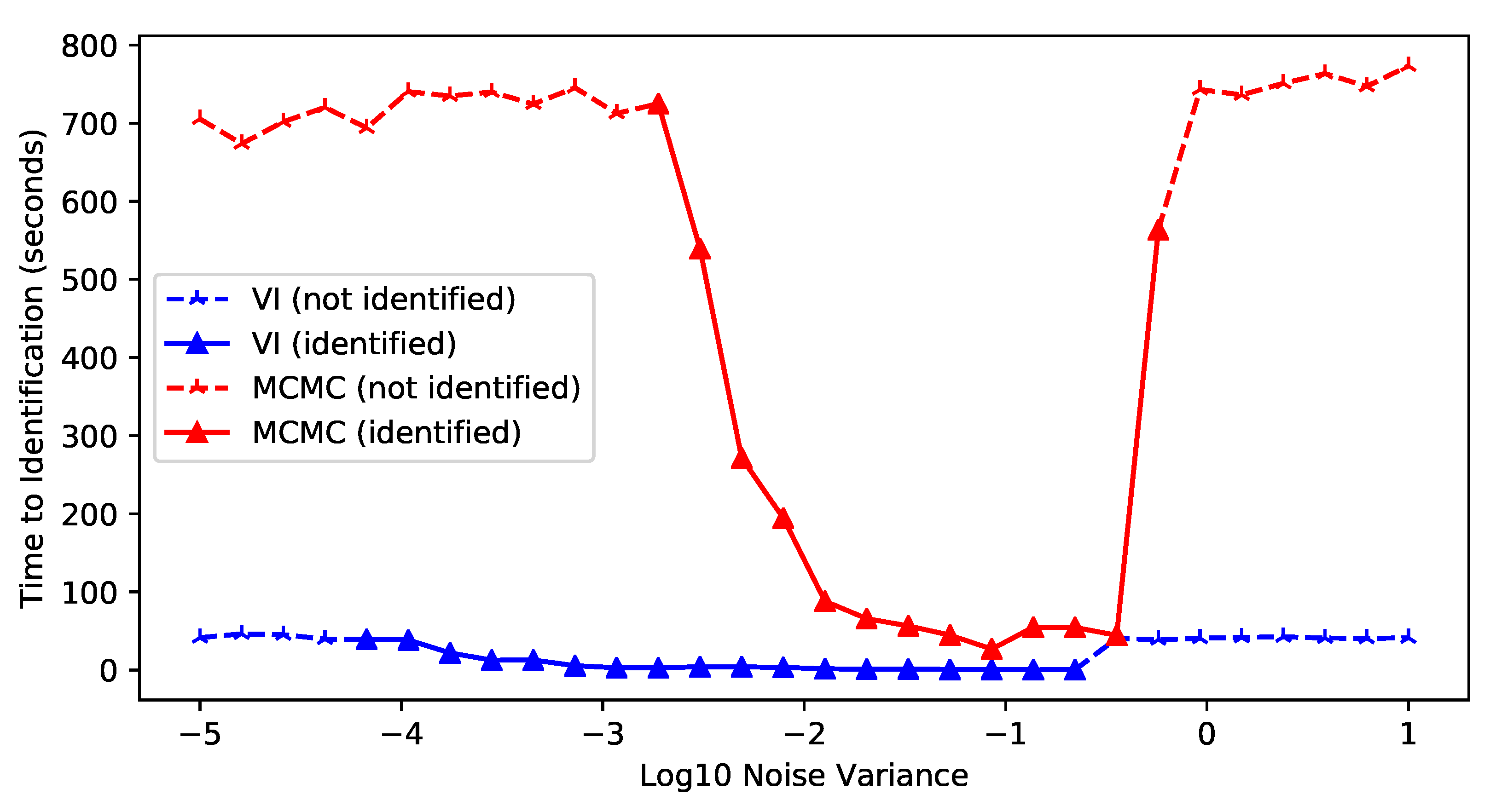
These results indicate that both MCMC sampling and VI become slower as noise decreases due to strong dependencies in the posterior. We hypothesize it is because both MCMC and VI suffer from the dependency introduced by low noise, which is a known long-standing issue with ongoing research methods, e.g., structured VI [72], or blocked/collapsed Gibbs sampler [74]. But both MCMC and VI work well provided there are sufficient iterations. This behavior suggests that the dependency induced by very low noise levels creates an optimization challenge rather than a fundamental modeling issue.
In summary: (1) VI is significantly faster than MCMC, (2) both methods slow down as the noise level decreases, and (3) both fail to recover the correct components when the noise is excessively high.
References
- Wang, J.L.; Chiou, J.M.; Müller, H.G. Functional Data Analysis. Annual Review of Statistics and Its Application 2016, 3, 257–295. [CrossRef]
- Ramsay, J.O.; Silverman, B.W. Applied functional data analysis: methods and case studies; Springer, 2002.
- Rice, J.A.; Silverman, B.W. Estimating the Mean and Covariance Structure Nonparametrically When the Data are Curves. Journal of the Royal Statistical Society Series B: Statistical Methodology 1991, 53, 233–243. [CrossRef]
- Górecki, T.; Krzyśko, M.; Waszak, .; Wołyński, W. Selected statistical methods of data analysis for multivariate functional data. Statistical Papers 2018, 59, 153–182. [CrossRef]
- Aneiros, G.; Cao, R.; Fraiman, R.; Genest, C.; Vieu, P. Recent advances in functional data analysis and high-dimensional statistics. Journal of Multivariate Analysis 2019, 170, 3–9. [CrossRef]
- Li, Y.; Qiu, Y.; Xu, Y. From multivariate to functional data analysis: Fundamentals, recent developments, and emerging areas. Journal of Multivariate Analysis 2022, 188, 104806. [CrossRef]
- Happ, C.; Greven, S. Multivariate Functional Principal Component Analysis for Data Observed on Different (Dimensional) Domains. Journal of the American Statistical Association 2018, 113, 649–659. [CrossRef]
- Kowal, D.R.; Canale, A. Semiparametric Functional Factor Models with Bayesian Rank Selection. Bayesian Analysis 2023, 18. [CrossRef]
- Paulon, G.; Müller, P.; Sarkar, A. Bayesian Semiparametric Hidden Markov Tensor Models for Time Varying Random Partitions with Local Variable Selection. Bayesian Analysis 2024, 19. [CrossRef]
- Goldsmith, J.; Zipunnikov, V.; Schrack, J. Generalized Multilevel Function-on-Scalar Regression and Principal Component Analysis. Biometrics 2015, 71, 344–353. [CrossRef]
- Nguyen, X.; Gelfand, A.E. The Dirichlet labeling process for clustering functional data. Statistica Sinica 2011, 21, 1249–1289. [CrossRef]
- Petrone, S.; Guindani, M.; Gelfand, A.E. Hybrid Dirichlet Mixture Models for Functional Data. Journal of the Royal Statistical Society Series B: Statistical Methodology 2009, 71, 755–782. [CrossRef]
- Berrendero, J.; Justel, A.; Svarc, M. Principal components for multivariate functional data. Computational Statistics & Data Analysis 2011, 55, 2619–2634. [CrossRef]
- Suarez, A.J.; Ghosal, S. Bayesian Estimation of Principal Components for Functional Data. Bayesian Analysis 2017, 12. [CrossRef]
- Yang, J.; Zhu, H.; Choi, T.; Cox, D.D. Smoothing and Mean–Covariance Estimation of Functional Data with a Bayesian Hierarchical Model. Bayesian analysis 2016/09, 11, 649–670. [CrossRef]
- Fox, E.B.; Dunson, D.B. Bayesian nonparametric covariance regression. The Journal of Machine Learning Research 2015, 16, 2501–2542.
- Goldsmith, J.; Wand, M.P.; Crainiceanu, C. Functional regression via variational Bayes. Electronic journal of statistics 2011/01/01, 5, 572–602. [CrossRef]
- Sun, T.Y.; Kowal, D.R. Ultra-Efficient MCMC for Bayesian Longitudinal Functional Data Analysis. Journal of Computational and Graphical Statistics 2024, pp. 1–13. [CrossRef]
- Rasmussen, C.E.; Williams, C.K.I. Gaussian processes for machine learning; Adaptive computation and machine learning, MIT Press: Cambridge, Mass, 2006; p. 248.
- Yao, F.; Müller, H.G.; Wang, J.L. Functional Data Analysis for Sparse Longitudinal Data. Journal of the American Statistical Association 2005, 100, 577–590. [CrossRef]
- Di, C.Z.; Crainiceanu, C.M.; Caffo, B.S.; Punjabi, N.M. Multilevel functional principal component analysis. The Annals of Applied Statistics 2009, 3, 458–488. [CrossRef]
- Peng, J.; Paul, D. A geometric approach to maximum likelihood estimation of the functional principal components from sparse longitudinal data. Journal of Computational and Graphical Statistics 2009, 18, 995–1015.
- Goldsmith, J.; Schwartz, J.E. Variable selection in the functional linear concurrent model. Statistics in Medicine 2017/06/30, 36, 2237–2250. [CrossRef]
- Xiao, L.; Li, C.; Checkley, W.; Crainiceanu, C. Fast covariance estimation for sparse functional data. Statistics and Computing 2018, 28, 511–522. [CrossRef]
- Chiou, J.M.; Yang, Y.F.; Chen, Y.T. Multivariate functional principal component analysis: A normalization approach. Statistica Sinica 2014. [CrossRef]
- Jacques, J.; Preda, C. Model-based clustering for multivariate functional data. Computational Statistics & Data Analysis 2014, 71, 92–106. [CrossRef]
- Yang, J.; Cox, D.D.; Lee, J.S.; Ren, P.; Choi, T. Efficient Bayesian Hierarchical Functional Data Analysis with Basis Function Approximations Using Gaussian–Wishart Processes. Biometrics 2017/12/01, 73, 1082–1091. [CrossRef]
- Trefethen, L.N. Approximation theory and approximation practice, extended edition; SIAM, 2019.
- Bungartz, H.J.; Griebel, M. Sparse grids. Acta numerica 2004, 13, 147–269.
- Zipunnikov, V.; Caffo, B.; Yousem, D.M.; Davatzikos, C.; Schwartz, B.S.; Crainiceanu, C. Multilevel functional principal component analysis for high-dimensional data. Journal of Computational and Graphical Statistics 2011, 20, 852–873. [CrossRef]
- Yao, F.; Lei, E.; Wu, Y. Effective dimension reduction for sparse functional data. Biometrika 2015, 102, 421–437. [CrossRef]
- Shi, H.; Yang, Y.; Wang, L.; Ma, D.; Beg, M.F.; Pei, J.; Cao, J. Two-Dimensional Functional Principal Component Analysis for Image Feature Extraction. Journal of Computational and Graphical Statistics 2022, 31, 1127–1140. [CrossRef]
- Van Der Linde, A. Variational Bayesian functional PCA. Computational Statistics & Data Analysis 2008, 53, 517–533. [CrossRef]
- Montagna, S.; Tokdar, S.T.; Neelon, B.; Dunson, D.B. Bayesian Latent Factor Regression for Functional and Longitudinal Data. Biometrics 2012, 68, 1064–1073. [CrossRef]
- Kowal, D.R.; Bourgeois, D.C. Bayesian Function-on-Scalars Regression for High-Dimensional Data. Journal of Computational and Graphical Statistics 2020-7-2, 29, 629–638. [CrossRef]
- Sousa, P.H.T.O.; Souza, C.P.E.d.; Dias, R. Bayesian adaptive selection of basis functions for functional data representation. Journal of Applied Statistics 2024-04-03, 51, 958–992. [CrossRef]
- Li, Y.; Wang, N.; Carroll, R.J. Selecting the Number of Principal Components in Functional Data. Journal of the American Statistical Association 2013, 108, 1284–1294. [CrossRef]
- Huang, L.; Reiss, P.T.; Xiao, L.; Zipunnikov, V.; Lindquist, M.A.; Crainiceanu, C.M. Two-way principal component analysis for matrix-variate data, with an application to functional magnetic resonance imaging data. Biostatistics 2017, 18, 214–229. [CrossRef]
- Lynch, B.; Chen, K. A test of weak separability for multi-way functional data, with application to brain connectivity studies. Biometrika 2018, 105, 815–831. [CrossRef]
- Shamshoian, J.; Şentürk, D.; Jeste, S.; Telesca, D. Bayesian analysis of longitudinal and multidimensional functional data. Biostatistics 2022/04/13, 23, 558–573. [CrossRef]
- Huo, S.; Morris, J.S.; Zhu, H. Ultra-Fast Approximate Inference Using Variational Functional Mixed Models. Journal of Computational and Graphical Statistics 2023-4-3, 32, 353–365. [CrossRef]
- Jolliffe, I.T.; Cadima, J. Principal component analysis: a review and recent developments. Philosophical Transactions of the Royal Society A: Mathematical, Physical and Engineering Sciences 2016, 374, 20150202. [CrossRef]
- Tipping, M.E.; Bishop, C.M. Probabilistic principal component analysis. Journal of the Royal Statistical Society Series B: Statistical Methodology 1999, 61, 611–622.
- Ilin, A.; Raiko, T. Practical approaches to principal component analysis in the presence of missing values. The Journal of Machine Learning Research 2010, 11, 1957–2000.
- Bishop, C. Bayesian pca. Advances in neural information processing systems 1998, 11.
- Tipping, M.E.; Bishop, C.M. Mixtures of probabilistic principal component analyzers. Neural computation 1999, 11, 443–482. [CrossRef]
- Minka, T. Automatic choice of dimensionality for PCA. Advances in neural information processing systems 2000, 13.
- Li, J.; Tao, D. On Preserving Original Variables in Bayesian PCA With Application to Image Analysis. IEEE Transactions on Image Processing 2012, 21, 4830–4843. [CrossRef]
- Bouveyron, C.; Latouche, P.; Mattei, P.A. Bayesian variable selection for globally sparse probabilistic PCA. Electronic Journal of Statistics 2018, 12. [CrossRef]
- Ning, Y.C.B.; Ning, N. Spike and slab Bayesian sparse principal component analysis. Statistics and Computing 2024, 34, 118.
- Bhattacharya, A.; Dunson, D.B. Sparse Bayesian infinite factor models. Biometrika 2011, 98, 291–306. [CrossRef]
- Tipping, M.E. Sparse Bayesian learning and the relevance vector machine. Journal of machine learning research 2001, 1, 211–244.
- Tipping, M. The relevance vector machine. Advances in neural information processing systems 1999, 12.
- Faul, A.C.; Tipping, M.E., Analysis of Sparse Bayesian Learning. In Advances in Neural Information Processing Systems 14; The MIT Press, 2002; pp. 383–390.
- MacKay, D.J., Bayesian methods for backpropagation networks. In Models of neural networks III: association, generalization, and representation; Springer, 1996; pp. 211–254.
- Neal, R.M. Bayesian learning for neural networks; Vol. 118, Springer Science & Business Media, 2012.
- Palmer, J.; Rao, B.; Wipf, D. Perspectives on sparse Bayesian learning. Advances in neural information processing systems 2003, 16.
- Wipf, D.; Nagarajan, S. A new view of automatic relevance determination. Advances in neural information processing systems 2007, 20.
- Wipf, D.; Rao, B. ℓ0-norm minimization for basis selection. In Proceedings of the Proceedings of the 17th International Conference on Neural Information Processing Systems, 2004, pp. 1513–1520.
- Wipf, D.P.; Rao, B.D.; Nagarajan, S. Latent Variable Bayesian Models for Promoting Sparsity. IEEE Transactions on Information Theory 2011, 57, 6236–6255. [CrossRef]
- Wipf, D.; Rao, B. Sparse Bayesian Learning for Basis Selection. IEEE Transactions on Signal Processing 2004, 52, 2153–2164. [CrossRef]
- Bishop, C.M. Variational Principal Components. In Proceedings of the Proceedings Ninth International Conference on Artificial Neural Networks, ICANN’99. IEE, 1999, pp. 509–514.
- Nakajima, S.; Sugiyama, M.; Babacan, D. On Bayesian PCA: Automatic dimensionality selection and analytic solution. In Proceedings of the Proceedings of the 28th International Conference on Machine Learning (ICML-11), 2011, pp. 497–504.
- Girolami, M.; Rogers, S. Hierarchic Bayesian models for kernel learning. In Proceedings of the Proceedings of the 22nd international conference on Machine learning, 2005, pp. 241–248.
- Bishop, C.M.; Tipping, M.E. Variational relevance vector machines. In Proceedings of the Proceedings of the Sixteenth conference on Uncertainty in artificial intelligence, 2000, pp. 46–53.
- Cheng, L.; Yin, F.; Theodoridis, S.; Chatzis, S.; Chang, T.H. Rethinking Bayesian Learning for Data Analysis: The Art of Prior and Inference in Sparsity-Aware Modeling. IEEE Signal Processing Magazine 2022, 39, 18–52. [CrossRef]
- Qi, Y.A.; Minka, T.P.; Picard, R.W.; Ghahramani, Z. Predictive automatic relevance determination by expectation propagation. In Proceedings of the Twenty-first international conference, Banff, Alberta, Canada, 2004; p. 85. [CrossRef]
- Babacan, S.D.; Luessi, M.; Molina, R.; Katsaggelos, A.K. Sparse Bayesian Methods for Low-Rank Matrix Estimation. IEEE Transactions on Signal Processing 2012, 60, 3964–3977. [CrossRef]
- Zhao, Q.; Meng, D.; Xu, Z.; Zuo, W.; Yan, Y. L1 -Norm Low-Rank Matrix Factorization by Variational Bayesian Method. IEEE Transactions on Neural Networks and Learning Systems 2015, 26, 825–839. [CrossRef]
- Guan, Y.; Dy, J. Sparse probabilistic principal component analysis. In Proceedings of the Artificial Intelligence and Statistics. PMLR, 2009, pp. 185–192.
- Wong, A.P.S.; Wijffels, S.E.; Riser, S.C.; Pouliquen, S.; Hosoda, S.; Roemmich, D.; Gilson, J.; Johnson, G.C.; Martini, K.; Murphy, D.J.; et al. Argo Data 1999-2019: Two Million Temperature-Salinity Profiles and Subsurface Velocity Observations From a Global Array of Profiling Floats. Frontiers in Marine Science 2020, 7, 700. [CrossRef]
- Blei, D.M.; Kucukelbir, A.; McAuliffe, J.D. Variational Inference: A Review for Statisticians. Journal of the American Statistical Association 2017, 112, 859–877. [CrossRef]
- Tipping, M.E.; Faul, A.C. Fast marginal likelihood maximisation for sparse Bayesian models. In Proceedings of the International workshop on artificial intelligence and statistics. PMLR, 2003, pp. 276–283.
- Park, T.; Lee, S. Improving the Gibbs sampler. Wiley Interdisciplinary Reviews: Computational Statistics 2022, 14, e1546.
- Ledoit, O.; Wolf, M. A well-conditioned estimator for large-dimensional covariance matrices. Journal of Multivariate Analysis 2004, 88, 365–411. [CrossRef]
- Kaslow, R.A.; Ostrow, D.G.; Detels, R.; Phair, J.P.; Polk, B.F.; RINALDO Jr, C.R.; Study, M.A.C. The Multicenter AIDS Cohort Study: rationale, organization, and selected characteristics of the participants. American journal of epidemiology 1987, 126, 310–318. [CrossRef]
- Argo float data and metadata from Global Data Assembly Centre (Argo GDAC) - Snapshot of Argo GDAC of November 09st 2024, 2024. [CrossRef]
- Yarger, D.; Stoev, S.; Hsing, T. A functional-data approach to the Argo data. The Annals of Applied Statistics 2022, 16, 216–246. [CrossRef]
- de Boyer Montégut, C.; Madec, G.; Fischer, A.S.; Lazar, A.; Iudicone, D. Mixed layer depth over the global ocean: An examination of profile data and a profile-based climatology. Journal of Geophysical Research: Oceans 2004, 109.
- Roemmich, D.; Gilson, J. The 2004–2008 mean and annual cycle of temperature, salinity, and steric height in the global ocean from the Argo Program. Progress in oceanography 2009, 82, 81–100. [CrossRef]
- Kuusela, M.; Stein, M.L. Locally stationary spatio-temporal interpolation of Argo profiling float data. Proceedings of the Royal Society A 2018, 474, 20180400. [CrossRef]
Figure 1.
Probabilistic graphical model for the full model.
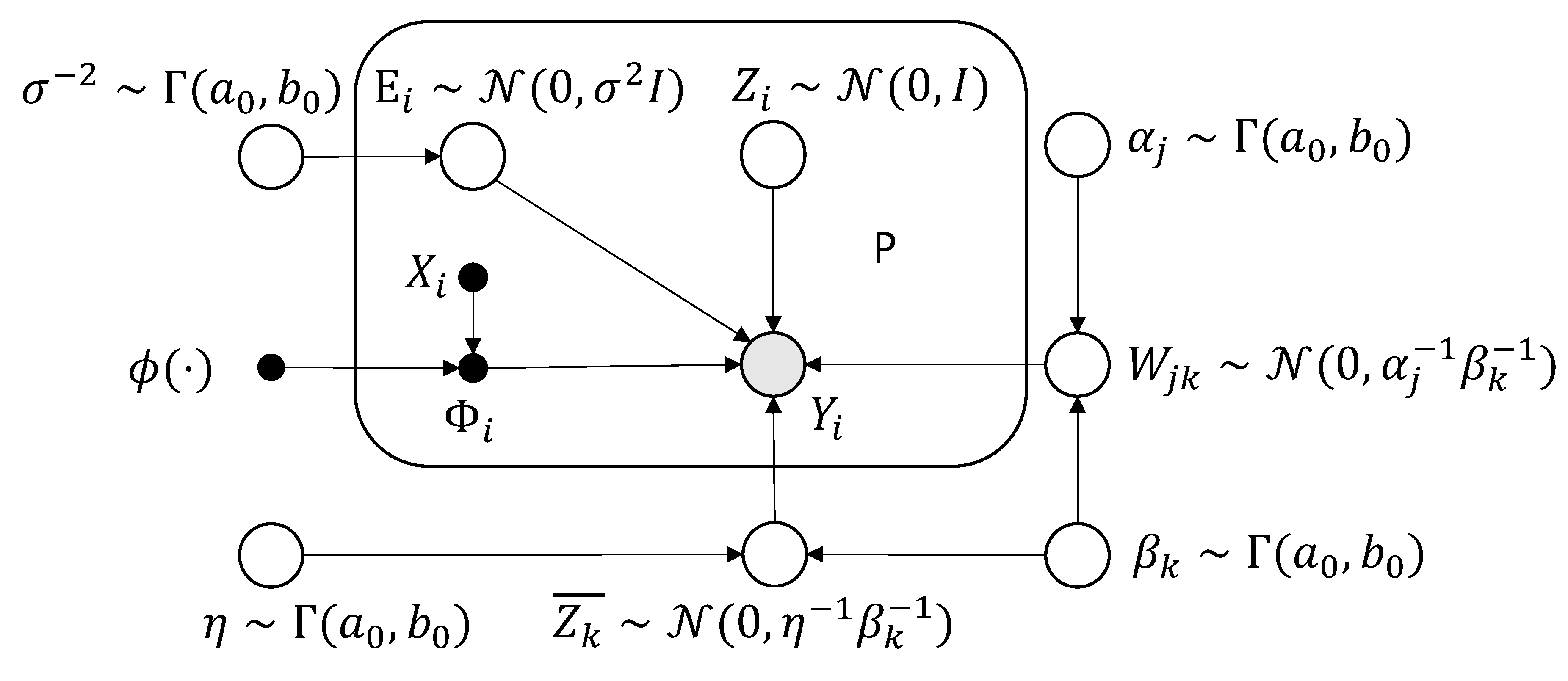
Figure 2.
Diagrams of variational inference algorithm for all the parameters. The top 3 diagrams each has a closed loop and a closed form overall transfer function.
Figure 2.
Diagrams of variational inference algorithm for all the parameters. The top 3 diagrams each has a closed loop and a closed form overall transfer function.
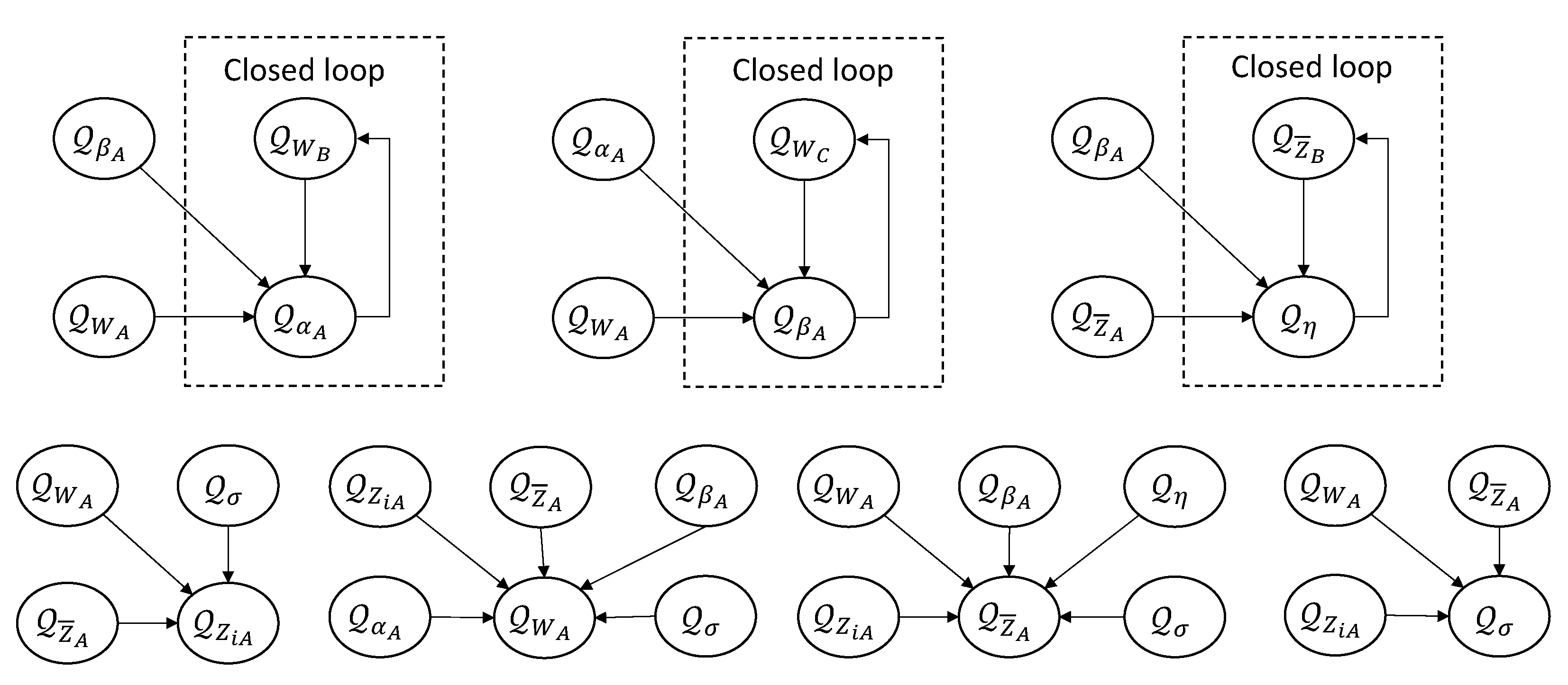
Figure 3.
length-scales and centers of selected kernel basis functions in a random repetition for three different m values in Scenario 5.
Figure 3.
length-scales and centers of selected kernel basis functions in a random repetition for three different m values in Scenario 5.
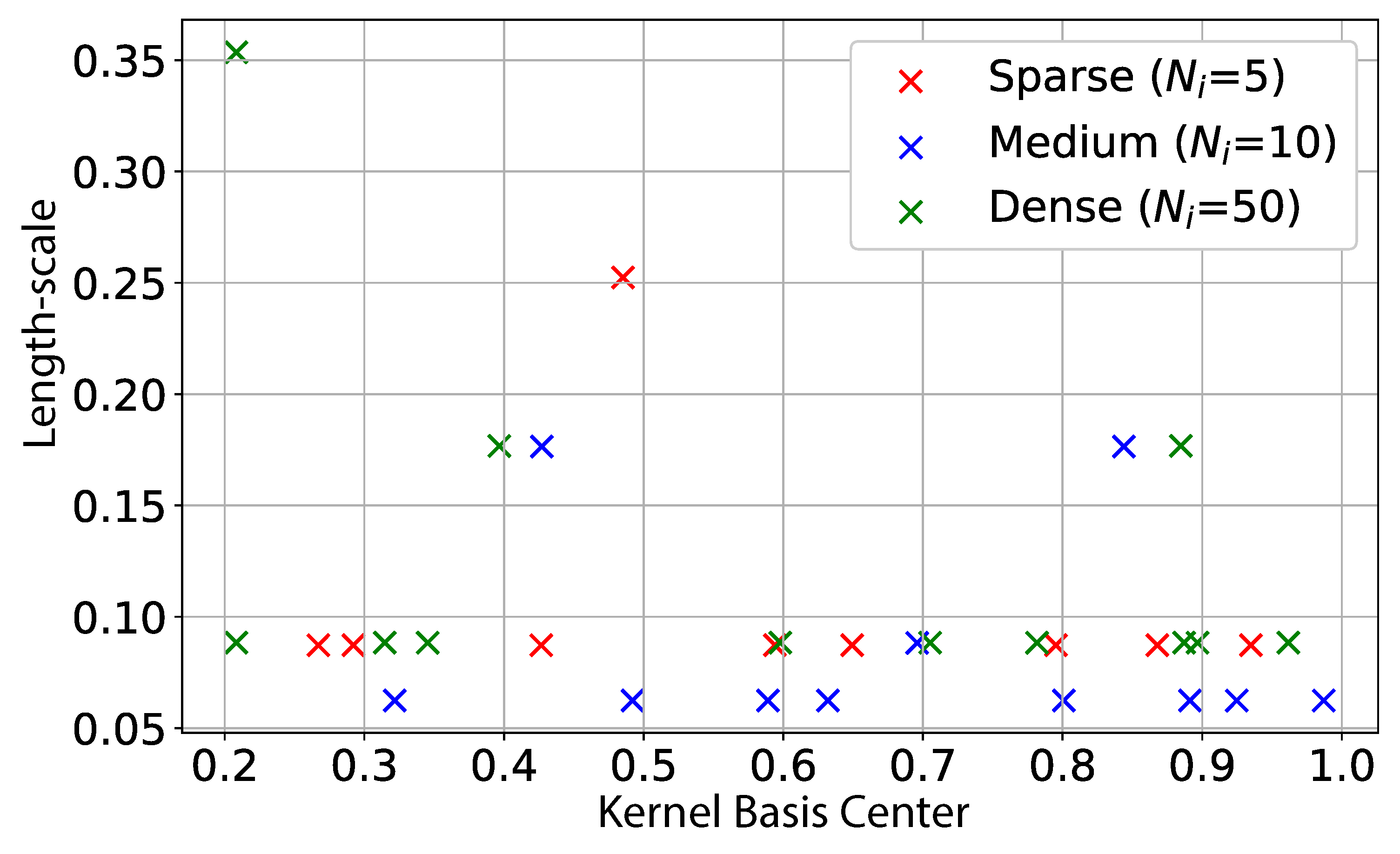
Figure 4.
Cross-sectional visualization of eigenfunctions (eigenvalues) of the 4D simulation.
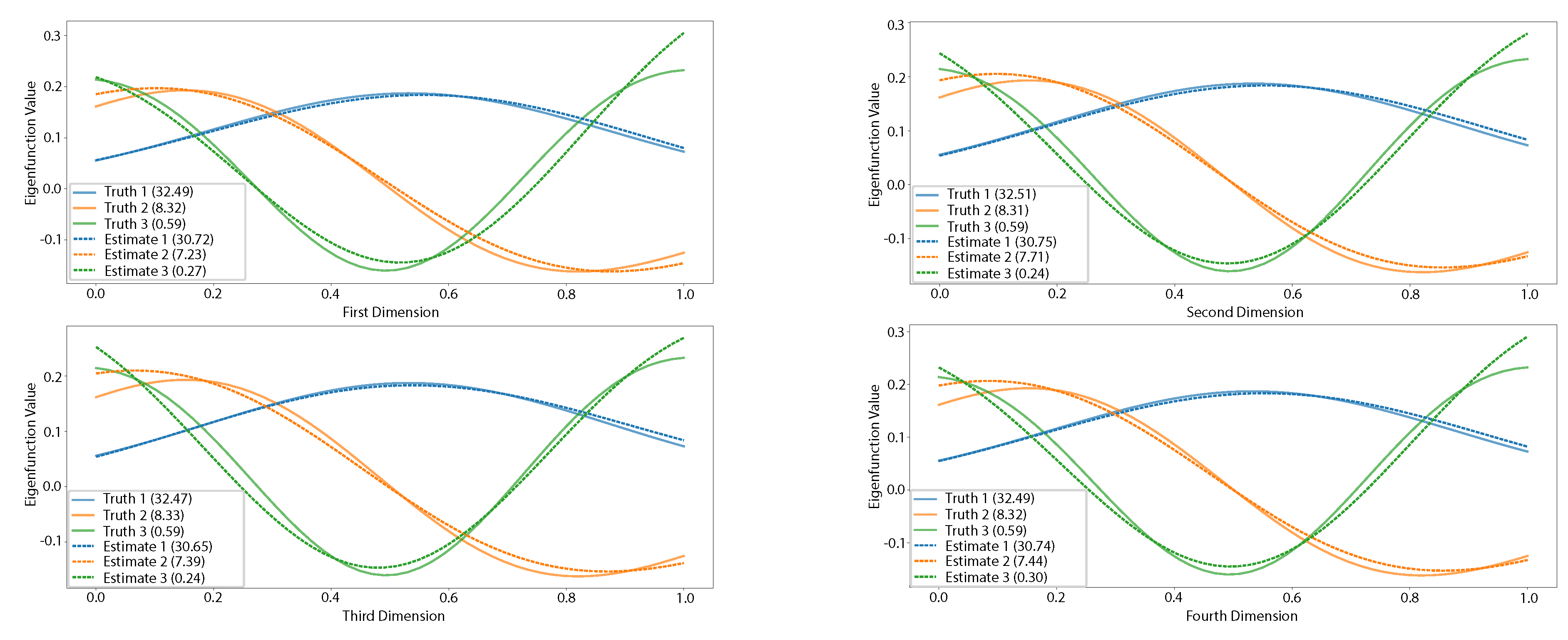
Figure 6.
Outcomes from the proposed method applied to MACS CD4 data sets.(top): Estimated curves for a random selection of 9 sampled functions and mean function; (bottom): Estimated eigenfunctions (eigenvalues).
Figure 6.
Outcomes from the proposed method applied to MACS CD4 data sets.(top): Estimated curves for a random selection of 9 sampled functions and mean function; (bottom): Estimated eigenfunctions (eigenvalues).
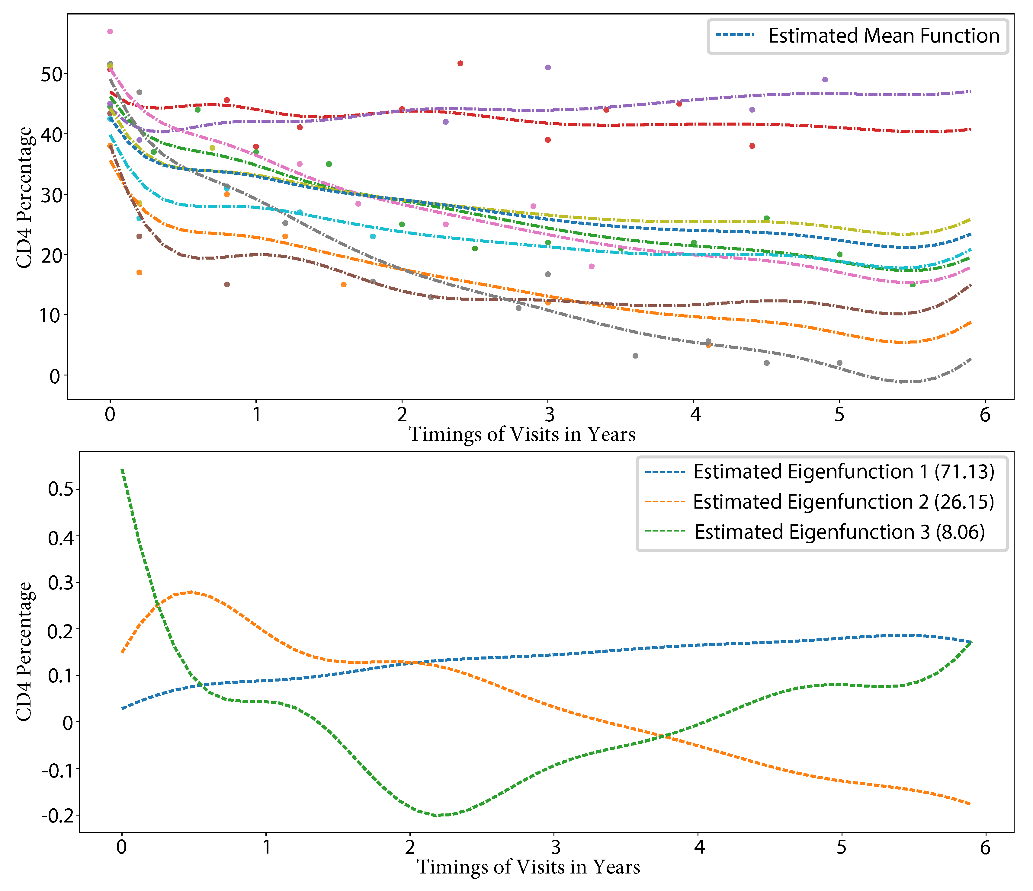
Figure 7.
Outcomes from the proposed method applied to a wind speed data set. (a) Estimated curves for a random selection of 9 sampled functions and mean function; (b) Estimated eigenfunctions (eigenvalues) denoted as EF; (c) Estimated covariance.
Figure 7.
Outcomes from the proposed method applied to a wind speed data set. (a) Estimated curves for a random selection of 9 sampled functions and mean function; (b) Estimated eigenfunctions (eigenvalues) denoted as EF; (c) Estimated covariance.
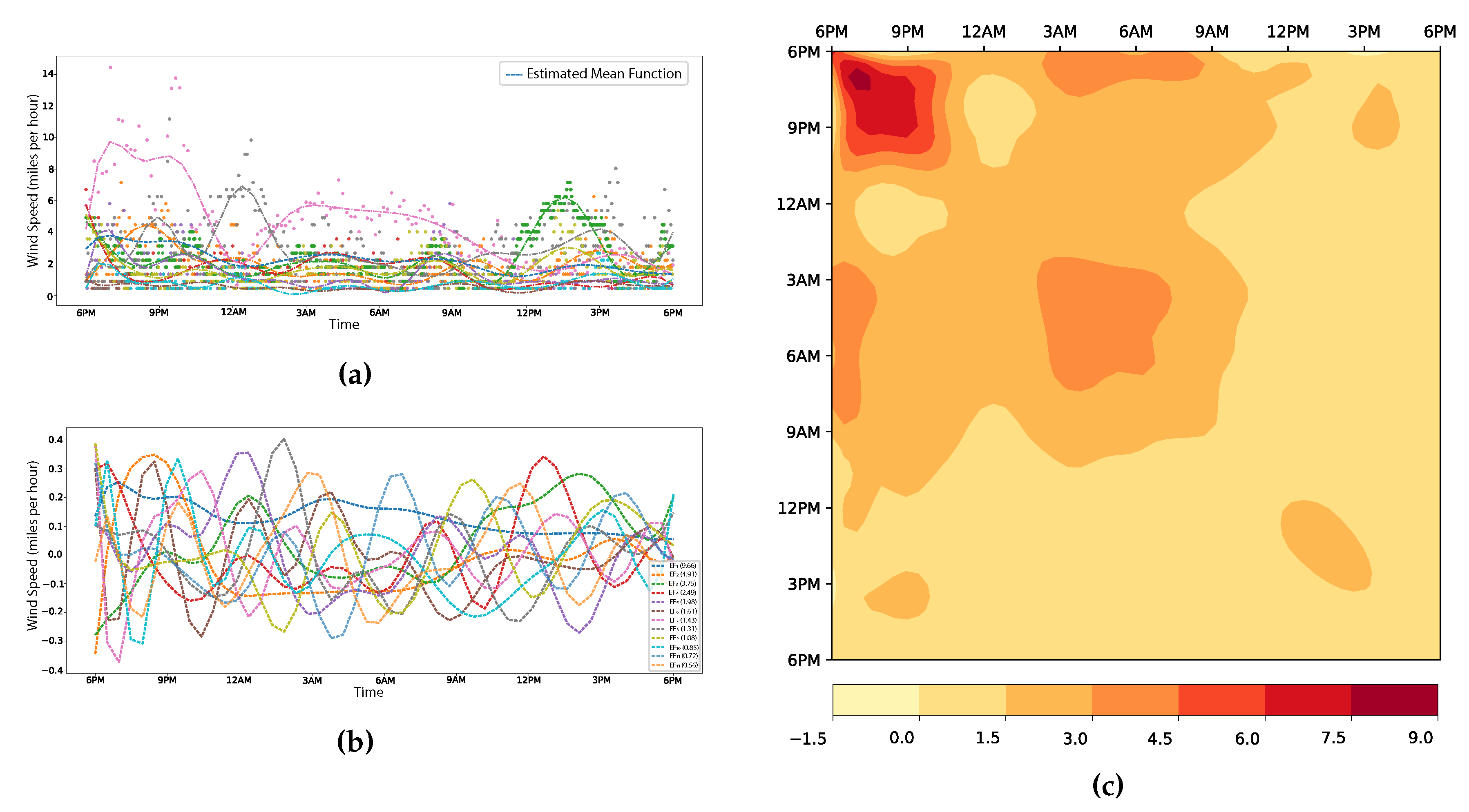
Figure 8.
Temperature measurements in 2021 February near the sea surface in the ARGO dataset.
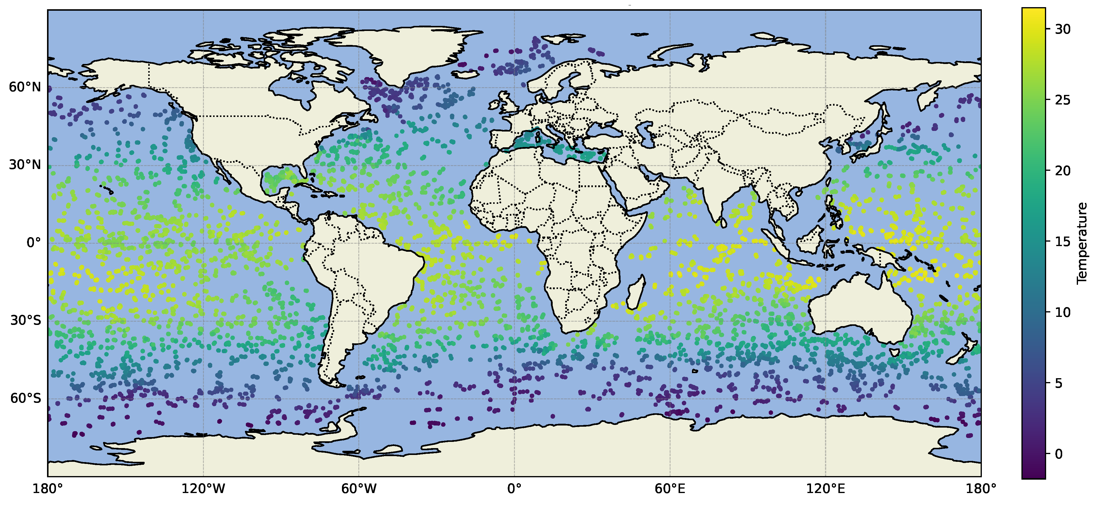
Figure 9.
Geodesic interpolation from vs. actual ARGO global oceanic measurements at 1, 200, and 300 decibars, at 1°S and 30°W on May 29. Measurements are represented by circles, with filling color indicating temperature. Circle sizes show distance in depth and time from the central point.
Figure 9.
Geodesic interpolation from vs. actual ARGO global oceanic measurements at 1, 200, and 300 decibars, at 1°S and 30°W on May 29. Measurements are represented by circles, with filling color indicating temperature. Circle sizes show distance in depth and time from the central point.
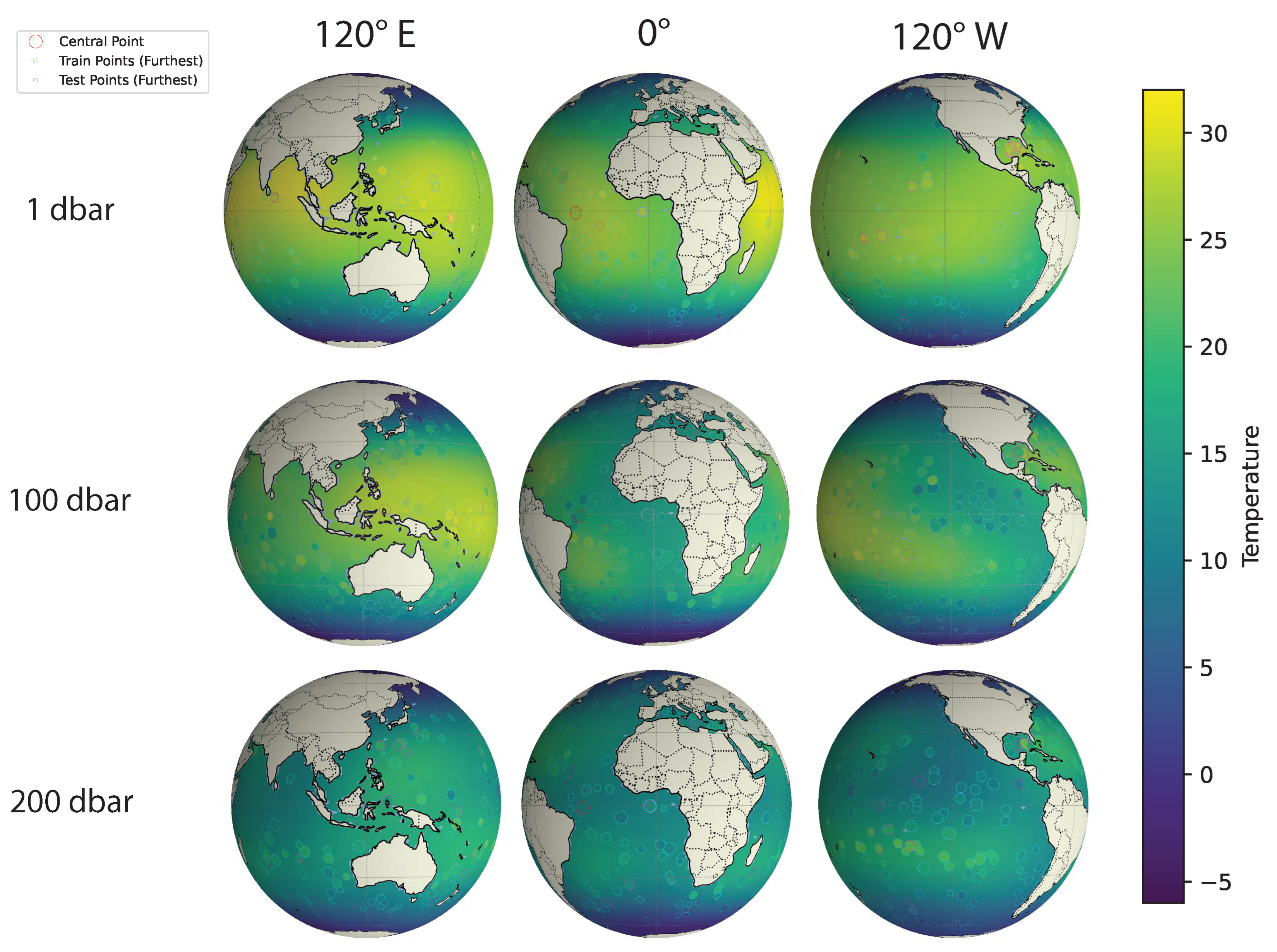
Figure 10.
Depth-time interpolation from vs. actual ARGO global oceanic measurements at two sites focusing on mixed layer behaviors. Measurements are represented by circles, with filling color indicating temperature. Circle sizes show distance in geodesic space from the central point.
Figure 10.
Depth-time interpolation from vs. actual ARGO global oceanic measurements at two sites focusing on mixed layer behaviors. Measurements are represented by circles, with filling color indicating temperature. Circle sizes show distance in geodesic space from the central point.
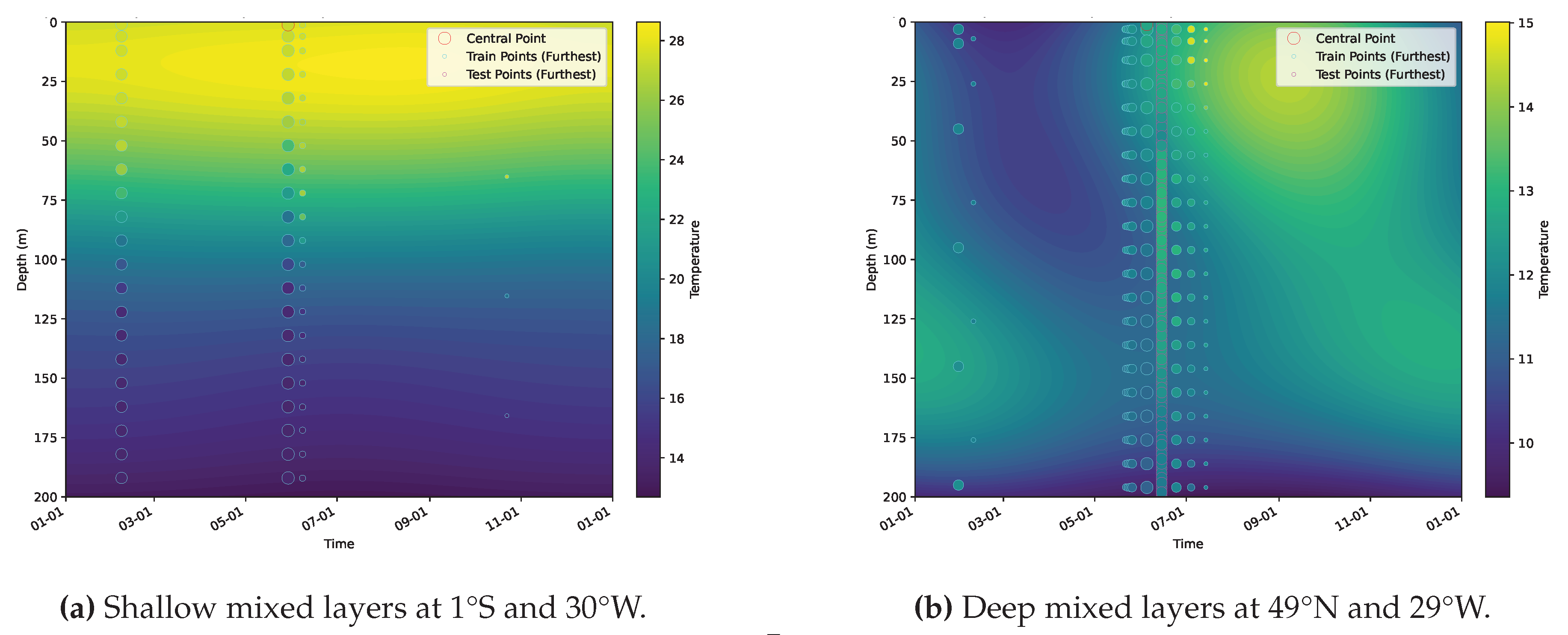
Table 1.
Proportion of accurate estimations for Scenario 1 (r=3).
| AIC | BIC | fpca | BSFDA | |||||||
| 5 | 0.000 | 0.580 | 0.380 | 0.410 | 0.735 | 0.650 | 0.880 | 0.645 | 0.995 | 0.015 |
| 10 | 0.000 | 0.980 | 0.670 | 0.955 | 0.985 | 0.880 | 0.920 | 0.645 | 1.000 | 0.910 |
| 50 | 0.000 | 1.000 | 0.830 | 1.000 | 1.000 | 1.000 | 1.000 | 0.890 | 0.980 | 0.945 |
Table 2.
Proportion of accurate estimations for Scenario 2 (r=3).
| AIC | BIC | fpca | BSFDA | |||||||
| 5 | 0.005 | 0.630 | 0.245 | 0.375 | 0.605 | 0.570 | 0.620 | 0.475 | 1.000 | 0.040 |
| 10 | 0.000 | 0.710 | 0.665 | 0.570 | 0.805 | 0.825 | 0.850 | 0.640 | 1.000 | 0.995 |
| 50 | 0.000 | 0.630 | 0.795 | 0.955 | 0.945 | 1.000 | 1.000 | 0.950 | 1.000 | 0.950 |
Table 3.
Proportion of accurate estimations for Scenario 3 (r=3).
| AIC | BIC | fpca | BSFDA | |||||||
| 5 | 0.005 | 0.720 | 0.325 | 0.640 | 0.590 | 0.320 | 0.400 | 0.450 | 0.995 | 0.945 |
| 10 | 0.000 | 0.580 | 0.770 | 0.965 | 0.665 | 0.740 | 0.755 | 0.440 | 0.995 | 1.000 |
| 50 | 0.000 | 1.000 | 0.775 | 1.000 | 1.000 | 1.000 | 1.000 | 0.765 | 0.980 | 0.920 |
Table 4.
Proportion of accurate estimations for Scenario 4 (r=3).
| AIC | BIC | fpca | BSFDA | |||||||
| 5 | 0.015 | 0.710 | 0.410 | 0.640 | 0.560 | 0.515 | 0.575 | 0.370 | 1.000 | 0.975 |
| 10 | 0.000 | 0.830 | 0.775 | 0.920 | 0.900 | 0.750 | 0.760 | 0.350 | 0.995 | 0.990 |
| 50 | 0.000 | 0.945 | 0.835 | 1.000 | 1.000 | 1.000 | 1.000 | 0.730 | 0.950 | 0.935 |
Table 5.
Proportion of accurate estimations for Scenario 5 (r=6).
| AIC | BIC | fpca | BSFDA | |||||||
| 5 | 0.705 | 0.470 | 0.090 | 0.070 | 0.545 | 0.425 | 0.410 | 0.855 | 0.925 | 0.160 |
| 10 | 0.065 | 0.570 | 0.525 | 0.775 | 0.705 | 0.575 | 0.575 | 0.500 | 1.000 | 0.930 |
| 50 | 0.000 | 0.260 | 0.590 | 0.980 | 0.965 | 0.870 | 0.770 | 0.695 | 0.995 | 0.925 |
Table 6.
Mean squared error of covariance for Scenario 5
| fpca | refund.sc | BSFDA | ||||
| 5 | 12.373 ± 4.026 | 12.377 ± 4.031 | 5.192 ± 6.166 | 8.833 ± 4.730 | 5.814 ± 3.535 | 10.292±12.717 |
| 10 | 10.391 ± 2.521 | 10.391 ± 2.521 | 2.098 ± 1.425 | 5.314 ± 3.501 | 2.068 ± 1.427 | 2.656±1.712 |
| 50 | 9.054 ± 1.683 | 9.054 ± 1.683 | 1.642 ± 1.240 | N/A | 1.638 ± 1.247 | 1.770±1.275 |
Disclaimer/Publisher’s Note: The statements, opinions and data contained in all publications are solely those of the individual author(s) and contributor(s) and not of MDPI and/or the editor(s). MDPI and/or the editor(s) disclaim responsibility for any injury to people or property resulting from any ideas, methods, instructions or products referred to in the content. |
© 2025 by the authors. Licensee MDPI, Basel, Switzerland. This article is an open access article distributed under the terms and conditions of the Creative Commons Attribution (CC BY) license (http://creativecommons.org/licenses/by/4.0/).
Copyright: This open access article is published under a Creative Commons CC BY 4.0 license, which permit the free download, distribution, and reuse, provided that the author and preprint are cited in any reuse.


