Preprint
Article

This version is not peer-reviewed.

Kernel-Based Independence Tests for Causal Structure Learning on Functional Data

A peer-reviewed article of this preprint also exists.

Submitted:

27 October 2023

Posted:

30 October 2023

You are already at the latest version

Abstract
Measurements of systems taken along a continuous functional dimension, such as time or space, are ubiquitous in many fields, from the physical and biological sciences to economics and engineering. Such measurements can be viewed as realisations of an underlying smooth process sampled over the continuum. However, traditional methods for independence testing and causal learning are not directly applicable to such data, as they do not take into account the dependence along the functional dimension. By using specifically designed kernels, we introduce statistical tests for bivariate, joint, and conditional independence for functional variables. Our method not only extends the applicability to functional data of the Hilbert-Schmidt independence criterion (HSIC) and its d-variate version (d-HSIC), but also allows us to introduce a test for conditional independence by defining a novel statistic for the conditional permutation test (CPT) based on the Hilbert-Schmidt conditional independence criterion (HSCIC), with optimised regularisation strength estimated through an evaluation rejection rate. Our empirical results of the size and power of these tests on synthetic functional data show good performance, and we then exemplify their application to several constraint- and regression-based causal structure learning problems, including both synthetic examples and real socio-economic data.
Keywords: 
;  ;  ;  

1. Introduction

Uncovering the causal relationships between measured variables, a discipline known as causal structure learning or causal discovery, is of great importance across various scientific fields, such as climatology [1], economics [2], or biology [3]. Doing so from passively collected (‘observational’) data enables the inference of causal interactions between variables without performing experiments or randomised control trials, which are often expensive, unethical, or impossible to conduct [4]. Causal structure learning is the inference, under a given set of assumptions, of directed and undirected edges in graphs representing the data generating process, where the nodes represent variables and the inferred edges capture causal (directed) or non-causal (undirected) relationships between them.
Much research in various areas collates functional data consisting of multiple series of measurements that are observed conjointly over a given continuum (e.g., time, space, or frequency), where each series is assumed to be a realisation of an underlying smooth process [5, §3]. By viewing the series of measurements as discretisations of functions, the observations are not required to be collected over regular meshes of points along the continuum. If the variables are measured over time as the underlying continuum, there is a long history of methods that have been developed to infer (time-based) causality between variables. Among those, the classic Granger-causality [6] declares that variable ‘X causes Y’ ( X Y ) if predicting the future of Y becomes more accurate with, as compared to without, access to the past of X, conditional on all other relevant variables. However, these methods assume that the observed time-series are stationary, the causal dependency of X on Y is linear, and no confounding variables are considered. More recently, Sugihara et al. [7] developed convergent cross mappings (ccms), a method that relaxes the assumption of linearity and finds causal relationships based on time-embeddings of the (stationary) time-series at each point, while also assuming no confounding variables are present. While useful in many situations, as we will show, Granger-causality and ccm can perform weakly when the time-series for X and Y are non-stationary and related through non-linear relationships, meaning that the influence of X on Y varies over time. Here we present a method that uses kernel-based independence tests to detect statistically significant causal relationships by extending constraint- and regression-based causal structure learning to functional data. The key advantage over Granger-causality and ccm is the consideration of confounders and the relaxation of their assumptions around linear relationships or stationarity in the data, which can lead to different causal relationships between variables. As a motivating example, consider the relationship between two variables: ‘corruption’ and ‘income inequality’, as measured by the World Governance Indicators (wgis) [8] and the World Bank [9], respectively. Using data for 48 African countries from 1996 to 2016, Sulemana and Kpienbaareh [2] investigated their cause-effect relationship and found that corruption ‘Granger-causes’ income inequality. Independently, we have also confirmed that applying ccm to the same data leads to the same conclusion. However, by considering the time-series data as realisations of functions over time, and thus avoiding linearity and stationarity assumptions, our proposed kernel-based approach suggests the reverse result, i.e., causal influence of income inequality on corruption appears as the more statistically likely direction. This is in agreement with other quantitative findings, which draw on different data sources [10,11,12]. We will return to this example in Section 4.2.2 where we analyse causal dependencies between all six wgis.
Methodologically, we extend the applicability of two popular paradigms in causal structure learning—constraint-based [13, § 5] and regression-based methods [14]—to functional data. Independence tests play a crucial role in uncovering causal relationships in both paradigms, and kernels provide a powerful framework for such tests by embedding probability distributions in reproducing kernel Hilbert space (rkhss) [15, § 2.2]. Until now, however, related methods for causal learning had only been applicable to univariate and multivariate data, but not to functional data. Here, we address this limitation by using recently derived kernels over functions [16] to embed probability distributions over functions in rkhss, thus widening the applicability of kernel-based independence tests to functional data settings. To test for conditional independence, we compute hscic [17] in a conditional permutation test (cpt) [18], and we propose a straightforward search to determine the optimised regularisation rate in hscic.
We structure our paper as follows. Section 2 provides a brief overview of prior literature on functional data analysis, kernel-based independence tests, and causal structure learning methods. Section 3 presents our methodological contributions, from the definition of a conditional independence test for functional data to causal structure learning on such data. We then empirically analyse the performance of our independence tests and causal structure learning algorithms on synthetic and real-world data in Section 4. We conclude with a discussion in Section 5.
We highlight the following contributions:
  • In Section 3 we propose a conditional independence test for functional data that combines a novel test statistic based on hscic with cpt to generate samples under the null hypothesis. The algorithm also searches for the optimised regularisation strength λ * required to compute hscic, by pre-test permutations and calculating an evaluation rejection rate.
  • In Section 4.1.2, we extend the historical functional linear model [19] to the multivariate case ( { X 1 , , X i , , X d } Y ) for regression-based causal structure learning, and we show how a joint independence test can be used to verify candidate directed acyclic graph (dags) [20, § 5.2] that embed the causal structure of function-valued random variables. This model has been contributed to the Python package scikit-fda [21].
  • On synthetic data, we show empirically that our bivariate, joint and conditional independence tests achieve high test power, and that our causal structure learning algorithms outperform previously proposed methods.
  • Using a real-world data set (World Governance Indicators) we demonstrate how our method can yield insights into cause-effect relationships amongst socio-economic variables measured in every country worldwide.
  • Implementations of our algorithms are made available at https://github.com/felix-laumann/causal-fda/ in an easily usable format that builds on top of scikit-fda and causaldag [22].

2. Background and Related Work

2.1. Functional Data Analysis

In functional data analysis [5], a variable X is described by a set of n samples (or realisations), X = { x i ( s ) } i = 1 n , where each functional sample x i ( s ) corresponds to a series of observations over the continuum s, also called the functional dimension. Typical functional dimensions are time or space. In practical settings, the observations are taken at a set of S discrete values s 1 , , s S of the continuum variable s. Examples of functional data sets include the vertical position of the lower lip over time when speaking out a given word [19], the muscle soreness over the duration of a tennis match [23], or the ultrafine particle concentration in air measured over the distance to the nearest motorway [24].
In applications, the functional samples are usually represented as linear combinations of a finite set of M basis functions { ϕ m ( s ) } m = 1 M (e.g., Fourier or monomial basis functions):
x i ( s ) = m = 1 M c i , m ϕ m ( s ) ,
where the coefficients C i = ( c i , 1 , c i , 2 , , c i , M ) characterise each sample. If the number of basis functions is equal to the number of observations, M = S , each observed value x i ( s k ) can be fitted exactly by obtaining the coefficients C i using standard non-linear least squares fitting techniques (provided the ϕ m ( s ) are valid basis functions), and Equation (1) allows us to interpolate between any two observations. When the number of basis functions is smaller than the number of observations, M < S , as it is commonly the case in practice, the basis function expansion (1) provides a smoothed approximation to the set of observations, x ^ i ( s k ) .
For the many applications where the continuum is time, historical functional linear model (hflms) [19] provide a comprehensive framework to map the relationship between two sets of functional samples. Let 0 and T be the initial and final time points for a set of samples y i ( t ) . hflms describe dependencies that can vary over time using the function β ( s , t ) , which encapsulates the influence of x ( s ) , s [ 0 , S ] on another variable y ( t ) , t [ 0 , T ] at any two points in time, s k and t k :
y i ( t ) = s 0 ( t ) t x i ( s ) β ( s , t ) d s , t [ 0 , T ]
where s 0 ( t ) is the maximum allowable lag for any influence of X on Y and s 0 ( t ) s t . Typical choices for β ( s , t ) are exponential decay and hyperbolic paraboloid (or “saddle”) functions. The continuum is not required to be time but can also be space, frequency or others (see Ramsay and Hooker [25] for an extensive collection of function-to-function models and applications).

2.2. Kernel Independence Tests

Let H k 1 and H k 2 be separable rkhss with kernels k 1 : R X × R X R and k 2 : R Y × R Y R such that the tensor product kernel ( k 1 k 2 ) ( x , y , x , y ) = k 1 ( x , x ) · k 2 ( y , y ) implies ( R X × R Y ) × ( R X × R Y ) R . If the kernel k 1 uniquely embeds a distribution P X in an rkhs by a mean embedding,
μ X : = X k 1 ( x , · ) d P X
which captures any information about P X , we call k 1 a characteristic kernel on R X × R Y [26]. Characteristic kernels have thus been extensively used in bivariate ( P X Y = P X P Y ), joint ( P X Y Z = P X P Y P Z ) and conditional ( P X Y | Z = P X | Z P Y | Z ) independence tests [e.g., 20,27,28].
For the bivariate independence test, let P X Y denote the joint distribution of X and Y . Then hsic is defined as
HSIC ( k 1 , k 2 , P X Y ) : = μ X Y μ X μ Y k 1 k 2 2 0 , with equality iff P X Y = P X P Y .
We refer to Gretton et al. [27] for the definition of an estimator for finite samples that constitutes the test statistic in the bivariate independence test with null hypothesis H 0 : X Y . The test statistic is then computed on the original data ( X , Y ) and statistically compared to random permutations { ( X , Y p ) } p = 1 P under the null hypothesis.
For distributions with more than two variables, let P X 1 , X 2 , , X d denote the joint distribution on X 1 , X 2 , , X d . To test for joint independence we compute
d -HSIC ( k 1 , k 2 , , k d , P X 1 , X 2 , , X d ) : = μ X 1 , X 2 , , X d μ X 1 μ X 2 μ X d k 1 k 2 k d 2 0 with equality iff P X 1 , X 2 , , X d = P X 1 P X 2 P X d .
Pfister et al. [20] derive a numerical estimator, which serves as the basis for a joint independence test on finite samples. Here, the distribution under the null hypothesis of joint independence is generated by randomly permuting all sample sets in the same way as Y is in the bivariate independence test.
Lastly, the conditional independence test relies on accurately sampling from the distribution under the null hypothesis H 0 : X Y | Z . At the core of the conditional permutation test [18] lies a randomisation procedure that generates permutations of X , denoted { X p } p = 1 P , which are generated without altering the conditional distribution P X | Z , so
P X p , Y , Z = P X , Y , Z
under H 0 while breaking any dependence between X and Y. The null distribution can therefore be generated by repeating this procedure multiple times, and we can decide whether H 0 should be rejected by comparing a test statistic on the original data against its results on the generated null distribution.
The existing literature on kernel-based independence tests is extensive, see e.g., Berrett et al. [18] for a relevant review, but only a small part of those tests investigates independence among functional variables [29,30]. There have been particularly strong efforts in developing conditional independence tests and understanding their applicable settings. The kernel conditional independence test (kcit) [28], for example, gave promising results in use with univariate data but increasingly suffered when the number of conditional variables was large. In contrast, the kernel conditional independence permutation test (kcipt) [31] repurposed the well-established kernel two-sample test [32] to a conditional independence setting which delivered stable results for multiple conditional variables. However, Lee and Honavar [33] pointed out that as the number of permutations increases, while its power increases, its calibratedness decreases. This issue was overcome by their proposed self-discrepancy conditional independence test (sdcit), which is based on a modified unbiased estimate of the maximum mean discrepancy (mmd).

2.3. Causal Structure Learning

The aim of causal structure learning, or causal discovery, is to infer the qualitative causal relationships among a set of observed variables, typically in the form of a causal diagram or dag. Once learnt, such a causal structure can then be used to construct a causal model such as a causal Bayesian network or a structural causal model (scm) [34]. Causal models are endowed with a notion of manipulation and, unlike a statistical model, do not just describe a single distribution, but many distributions indexed by different interventions and counterfactuals. They can be used for causal reasoning, that is, to answer causal questions such as computing the average causal effect of a treatment on a given outcome variable. Such questions are of interest across many disciplines, and causal discovery is thus a highly topical area. We refer to Glymour et al. [4], Mooij et al. [35], Peters et al. [36], Schölkopf and von Kügelgen [37], Squires and Uhler [38], Vowels et al. [39] for comprehensive surveys and accounts of the main research concepts. In particular, we focus here on causal discovery methods for causally sufficient systems, for which there are no unobserved confounders influencing two or more of the observed variables. Existing causal discovery methods can roughly be categorised into three families:
  • Score-based approaches assign a score, such as a penalised likelihood, to each candidate graph and then pick the highest scoring graph(s). A common drawback of score-based approaches is the need for a combinatorial enumeration of all dags in the optimisation, although greedy approaches have been proposed to alleviate such issues [40].
  • Constraint-based methods start by characterising the set of conditional independences in the observed data [13]. They then determine the graph(s) consistent with the detected conditional independences by using a graphical criterion called d-separation, as well as the causal Markov and faithfulness assumptions, which establish a one-to-one connection between d-separation and conditional independence (see Appendix D for definitions). When only observational i.i.d. data are available, this yields a so-called Markov equivalence class, possibly containing multiple candidate graphs. For example, the graphs X Y Z , X Y Z , and X Y Z are Markov equivalent, as they all imply X Z | Y and no other conditional independence relations.
  • Regression-based approaches directly fit the structural equations X i : = f i ( PA i , U i ) of an underlying scm for each X i , where PA i denote the parents of X i in the causal dag and U = ( U 1 , . . . , U n ) are jointly independent exogenous noise variables. Provided that the function class of the f i is sufficiently restricted, e.g., by considering only linear relationships [41] or additive noise models [42], the true causal graph is identified as the unique choice of parents for each i such that the resulting residuals U ^ i = X i f ^ i ( PA i ) are jointly independent.
As can be seen from these definitions, conditional, bivariate, and joint independence tests are an integral part of constraint- and regression-based causal discovery methods. Our main focus in the present work is therefore to extend the applicability of these causal discovery frameworks to functional data by generalising the underlying independence tests to such domains.

3. Methods

In all three of our independence tests (bivariate, joint, conditional), we employ kernels over functions, also known as squared-exponential T (se-t) kernels [16]. Let X and Y be real, separable Hilbert spaces with norms · X and · Y , respectively. Then, for T : X Y , se-t kernels are defined as
k T ( x , y ) = e 1 2 σ 2 T ( x ) T ( y ) Y 2 .
where σ 2 is commonly defined as the median heuristic, σ 2 = Median { T ( a ) T ( b ) Y 2 : a , b { x i } i = 1 n { y i } i = 1 n , a b } . Replacing any characteristic kernel by the se-t kernels for bivariate independence tests (based on hsic) and for joint independence tests (based on d-variable Hilbert-Schmidt independence criterion ( d -hsic)) is straightforward and does not require further theoretical investigation besides evaluating numerically the validity and power of the tests (see Section 4). However, the application of se-t kernels to conditional independence tests needs further theoretical results, as we discuss now.

3.1. Conditional Independence Test on Functional Data

We consider the conditional independence test, which generates samples under the null hypothesis based on the cpt, and uses the sum of hscics over all samples z Z as its test statistic. The cpt defines a permutation procedure that preserves the dependence of Z on both X and Y while resampling data for X that eliminates any potential dependence between X and Y. This procedure results in samples according to the null hypothesis, X Y | Z . We use this procedure whenever permutations are required as part of the conditional independence test. Given the computation of the hscic is based on a kernel ridge regression, it requires to set a regularisation strength λ , which has been manually chosen previously [17]. Generally, our aim is to have type-I error rates close to the allowable false positive rate α . However, choosing λ inappropriately may result in an invalid test (type-I error rates exceed α if λ is chosen too large), or in a deflated test power (type-I error rates are well below α and type-II error rates are high if λ is chosen too small). Thus, we must define an algorithm that conducts a search over a range of potentially suitable values for λ and assesses each candidate value by, what we will call, an evaluation rejection rate.
The search proceeds by iterating over a range of values { λ l } l = 1 L to find the optimised value λ * , as follows. For each λ l , we start by producing one permutation of the samples X , which we denote as X b , and we compute its corresponding evaluation test statistic given by the sum of hscics over all samples z Z . We then apply the usual strategy for permutation-based statistical tests: we produce an additional set of P permuted sample sets of X , which we denote { X π } π = 1 P , and for each X π , we determine the sum of hscics over z Z to generate a distribution over statistics under the null hypothesis, which we call the evaluation null statistics. We then compute the percentile where the evaluation test statistic on X b falls within the distribution of evaluation null statistics on the permutation set { X π } π = 1 P . This results in an evaluation p-value which is compared to the allowable false positive rate α to establish if the hypothesis H 0 : X b Y | Z can be rejected. Given that both the evaluation test statistic and the evaluation null statistics are computed on conditionally independent samples, we repeat this procedure for b = 1 , , B 100 times to estimate an evaluation rejection rate for each value of λ l . Having completed this procedure over all values { λ l } l = 1 L , we select the λ l that produces an evaluation rejection rate closest to α as the optimised regularisation strength, λ * . Finally, we apply a cpt-based conditional independence test using the optimised λ * to test the null hypothesis H 0 : X Y | Z . This entire procedure is summarised in Algorithm 1.
Algorithm 1 Search for λ * with subsequent conditional independence test
Require: 
Samples ( X , Y , Z ), Range { λ l } l = 1 L , Significance level α , Permutation iterations P, Rejection iterations B
Initialise: 
evaluation rejection rate [ λ * ] = 0
1:
for  1 l L  do                                                                                                                                                                                                                                  ▹Start: Search for λ *
2:
    for  1 b B  do
3:
        Permute X by cpt, call them X b
4:
         evaluation test statistic [ b ] z Z HSCIC ( X b , Y , Z , λ l )
5:
        for  1 π P  do
6:
           Permute X b by cpt, call them X b , π
7:
            evaluation null statistics [ b , π ] z Z h s c i c ( X b , π , Y , Z , λ l )
8:
         evaluation p -value 1
9:
                     percentile ( evaluation test statistic [ b ] , evaluation null statistics [ b , : ] )
10:
        if  evaluation p - value α  then
11:
           Fail to reject H 0 : X b Y | Z
12:
            rejects [ b ] = 0
13:
        else
14:
           Reject H 0 : X b Y | Z
15:
            rejects [ b ] = 1
16:
     evaluation rejection rate [ λ l ] mean 1 b B ( rejects )
17:
    if  | evaluation rejection rate [ λ * ] α | | evaluation rejection rate [ λ l ] α |  then
18:
         λ * λ l
19:
return  λ *                                                                                                                                                                                                                                          ▹End: Search for λ *      
20:
test statistic z Z HSCIC ( X , Y , Z , λ * )                                                                                                                                                     ▹Start: Conditional independence test
21:
for  1 p P  do
22:
    Permute X by cpt, call them X p
23:
     null statistics [ p ] z Z HSCIC ( X p , Y , Z , λ * )
24:
p -value 1 percentile ( test statistic , null statistics )
25:
if   p -value α  then
26:
    Fail to reject H 0 : X Y | Z
27:
else
28:
    Reject H 0 : X Y | Z
 
                                                                                                                                                                                                                                ▹End: Conditional independence test
The following Theorem 1 guarantees the consistency of the conditional independence test in Algorithm 1 with respect to the regularisation parameter λ .
Theorem 1.
Let H k 1 and H k 2 be separable RKHSs with kernels k 1 : R X × R X R and k 2 : R Y × R Y R such that the tensor product kernel k 1 k 2 : ( R X × R Y ) × ( R X × R Y ) R is a characteristic kernel on R X × R Y  [43]. If the regularisation parameter λ = λ n decays as n at a slower rate than n 1 / 2 , then the test based on the test statistic in Algorithm 1 (lines 19–27) is consistent.
Proof. 
See Appendix B.    □

3.2. Causal Structure Learning on Functional Data

To infer the existence of (directed) edges in an underlying causal graph G based on the joint data distribution P over a set of observed variables, we must assume that G and P are intrinsically linked. Spirtes et al. [13, § 2.3.3] define the faithfulness assumption, from which it follows that if two random variables are (conditionally) independent in the observed distribution P , then they are d-separated in the underlying causal graph G [34, § 1.2.3]. Using this fact, constraint-based causal structure learning methods [13, § 5] take advantage of bivariate and conditional independence tests to infer whether two nodes are d-separated in the underlying graph. These methods yield completed partially directed acyclic graphs (cpdags), which are graphs with undirected and/or directed edges. In contrast, regression-based methods [14], utilise the joint independence test to discover dags that have all edges oriented. We now describe both of these approaches in more detail.

3.2.1. Constraint-Based Causal Structure Learning

Constraint-based causal structure learning relies on performing conditional independence tests for each pair of variables, X and Y, conditioned on any possible subset of the remaining variables, that is, any subset within the power set of the d { X , Y } remaining variables Z 1 , Z 2 , , Z * . Therefore, for d variables we need to carry out 2 d 2 conditional independence tests for every pair of variables, which results in d 2 2 d 2 tests in total.
Conditional dependences found in the data can then be used to delete and orient edges in the graph G, as follows. We start with a complete graph with d nodes, where each node corresponds to one of the variables. The edge connecting X and Y is deleted if there exists a subset Z 1 of the d 2 remaining variables such that Z * Z 1 and X Y | Z 1 . If we then find another subset Z 2 , such that Z * Z 2 , Z 1 = Z 2 { Z * } , and for which X Y | Z 2 , we can orient the edges X Z and Y Z to form colliders (or v-structures), X Z * Y .
Based on these oriented edges, ‘Meek’s orientation rules’ defined by Meek [44] [see e.g., 36, § 7.2.1] can be applied to direct additional edges based on certain graphical compositions, as shown in Appendix F. Briefly, these rules follow from the avoidance of cycles, which would violate the acyclicity of a dag, and colliders, which violate the found conditional independence. Algorithms that implement these criteria are the SGS algorithm and the more efficient PC algorithm [13], which we summarise in Appendix F.

3.2.2. Regression-Based Causal Structure Learning

To carry out our regression-based causal learning, we choose additive noise models (anms), a special class of scms where the noise terms are assumed to be independent and additive. This assumption guarantees that the causal graph can be identified if the function f i is non-linear with Gaussian additive noise [42,45], a typical setting in functional data. Our model over the set of random variables { X } i = 1 d is given by:
X i : = f i ( PA i ) + U i ,
where the additive noise terms U i are jointly independent, i.e., any noise term U i is independent of any intersection of the other noise terms,
P ( j = 1 k U i j ) = j = 1 k P ( U i j ) , k d .
Based on these assumptions, we follow resit [Regression with Subsequent Independence Testing; 14], an approach to causal discovery that can be briefly described as follows. If we only have two variables X and Y, we start by assuming that the samples in Y are the effect and the samples in X are the cause. Therefore we write Y as a function f ^ Y of X plus some noise, and we test whether the residual r Y = Y f ^ Y ( X ) is independent of X . We then exchange the roles of assumed effect and assumed cause to obtain the residual r X = X f ^ X ( Y ) , which is tested for independence from Y . To overcome issues with finite samples and test power, Peters et al. [14] used the p-value of the independence tests as a measure of strength of independence, which we follow in our experiments in Section 4. Alternatively, one may determine the causal direction for this bivariate case by comparing both cause-effect directions with respect to a score defined by Bühlmann et al. [46].
For d variables, the joint independence test replaces the bivariate independence test. Firstly, we consider the set of candidate causal graphs, Γ = { G 1 , , G γ , , G Γ } , which contains every potential dag with d nodes. For each candidate dag, G γ , we regress each descendant X i on its parents PA i :
X i : = k PA i f ^ i , k ( X k ) + U i , i 1 , , d ,
and we compute the residuals r X i = X i k PA i f ^ i , k ( X k ) . We then apply the joint independence test to all d residuals. The candidate dag  G γ is accepted as the ‘true’ causal graph if the null hypothesis of joint independence amongst the residuals is not rejected. This process is repeated over all candidate causal graphs in the set Γ . Again, because in finite samples this procedure may not always lead to only one candidate dag being accepted, the one with the highest p-value is chosen [14].

4. Experiments

In practice, functional data analysis requires samples of continuous functions evaluated over a mesh of discrete observations. In our synthetic data, we consider the interval s = [ 0 , 1 ] for our functional dimension and draw 100 equally spaced points over s to evaluate the functions. For real-world data, we map the space in which the data live (e.g., the years 1996 to 2020) to the interval s = [ 0 , 1 ] and interpolate over the discrete measurement points. We then use this interpolation to evaluate the functional samples on 100 equally spaced points. Unless otherwise mentioned, henceforth we use se-t kernels with T = I where I is the identity matrix and σ 2 as the median heuristic, as previously defined in Section 3.

4.1. Evaluation of Independence Tests for Functional Data

Before applying our proposed independence tests to causal structure learning problems, we use appropriate synthetic data to evaluate their type-I error rate (test size) and type-II error rate (test power). Type-I errors are made when the samples are independent (achieved by setting a = 0 in our experiments below) but the test concludes that they are dependent, i.e., the test falsely rejects the null hypothesis H 0 . In contrast, type-II errors appear when the samples are dependent but the test fails to reject H 0 (achieved by setting a > 0 ). Specifically, we compute the error rates on 200 independent trials, which correspond to different random realisations of the data sets, i.e., synthetically generated data sets with random Fourier basis coefficients, random coefficients of the β -functions and random additive noise. We set the test significance level at α = 0.05 and approximate the null hypothesis of independence by 1000 permutations using the cpt scheme described above. Note that although our synthetic data are designed to replicate typical behaviour in time-series, the independence tests are not limited to time as the functional dimension, and can be used more generally.

4.1.1. Bivariate Independence Test

We consider n functional samples { x i ( s ) } i = 1 n of a random variable X defined over the interval s = [ 0 , 1 ] . To generate our samples, we sum M = 3 Fourier basis functions ϕ m , T ( s ) (definitions in Appendix A.1) with period T = 0.1 and coefficients c i , m randomly drawn from a standard normal distribution:
x i ( s ) = m = 1 M c i , m ϕ m , T ( s ) .
To mimic real-world measurements, we draw each sample over a distinct, irregular mesh of evaluation points. We then interpolate them with splines, and generate realisations over a regular mesh of points. Multivariate random noise ϵ i X ( s ) N ( 0 , I ) , where I is the identity matrix, is then added. The samples { y i ( t ) } i = 1 n of random variable Y are defined as a hflm[19] over t = [ 0 , 1 ] by:
y i ( t ) = a 0 t x i ( s ) β ( s , t ) d s ,
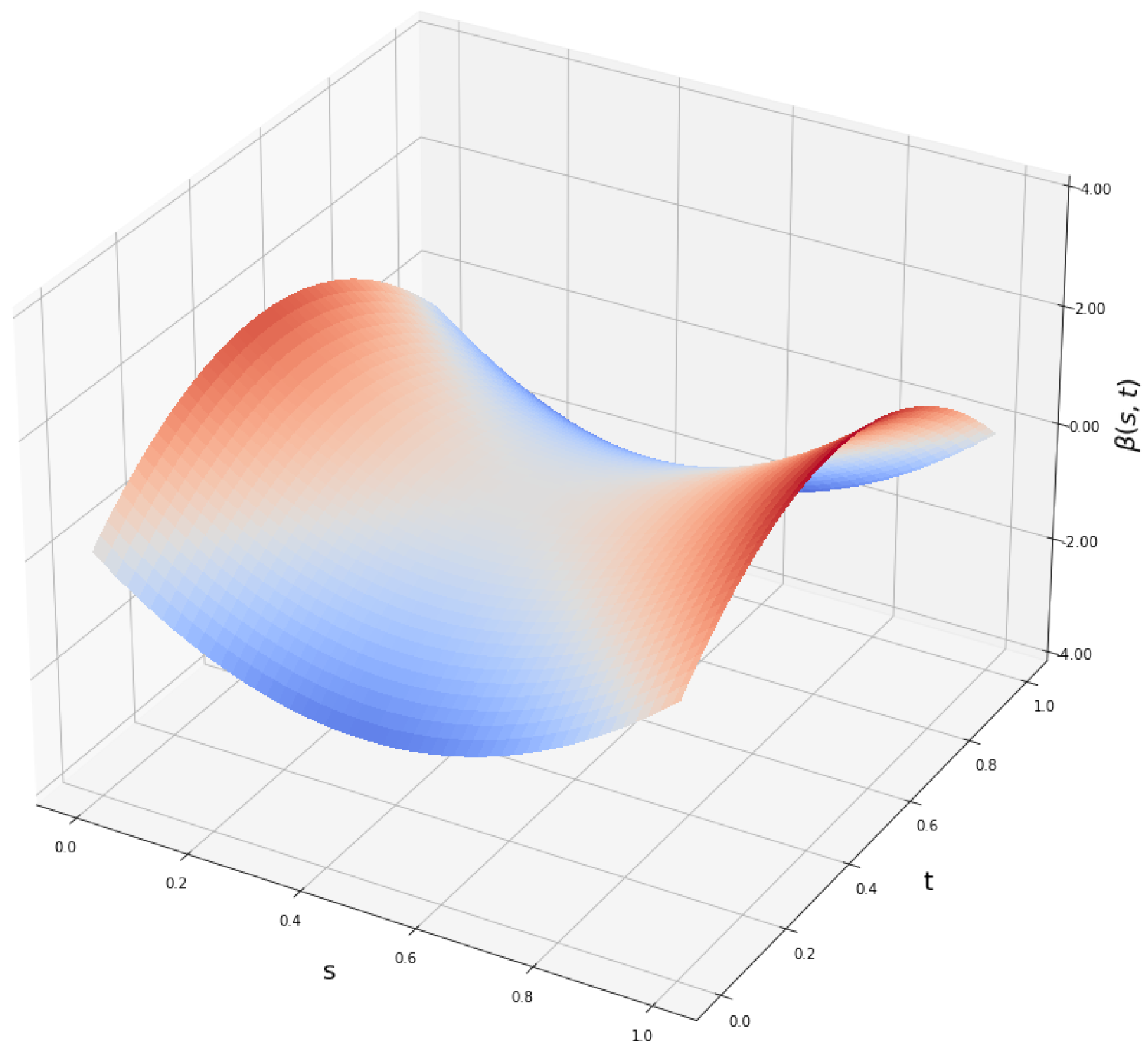
where a [ 0 , 1 ] . The function β ( s , t ) maps the dependence from x i at any point s to y i at any point t, and is defined here as a hyperbolic paraboloid function:
β ( s , t ) = 8 ( s c 1 ) 2 8 ( t c 2 ) 2 ,
with coefficients c 1 and c 2 drawn from uniform distributions (see Appendix A for lower and upper bounds). Afterwards, the samples y i ( t ) are evaluated over a regular mesh of 100 points t [ 0 , 1 ] and random noise ϵ i Y ( t ) N ( 0 , I ) is added. Clearly, for a = 0 our samples are independent, as the samples y i ( t ) = ϵ i Y ( t ) are just random noise. As a is increased, the dependence between the samples x i ( s ) and y i ( t ) becomes easier to detect. Figure 1 shows that our test has no difficulties in staying within the allowable false-positive rate α and quickly detects the dependence as soon as a > 0 even with very low number of samples.

4.1.2. Joint Independence Test

To produce the synthetic data for joint independence tests, we first generate random dags with d nodes using an Erdös-Rényi model with density 0.5 [20, § 5.2]. For each dag, we first use Equation (10) to produce function-valued random samples for the variables X i without parents. We then generate samples for other variables using a historical functional linear model:
x i j ( t ) = a p PA j 0 t x i p ( s ) β p ( s , t ) d s ,
where PA j are the parents of node X j , and the function β p ( s , t ) is given by Equation (12) with random coefficients c 1 and c 2 independently generated for each descendant-parent pair indexed by p. After being evaluated at a regular mesh of 100 points within t [ 0 , 1 ] , random noise ϵ i j ( t ) N ( 0 , I ) is added. Note that, again, an increase in the factor a [ 0 , 1 ] should make the dependence structure of the dag easier to detect. Figure 1 shows the test size where a = 0 , resulting in independent variables, and test power where a > 0 . We evaluate the joint independence test for d = 4 variables over various values of a and a range of sample sizes.

4.1.3. Conditional Independence Test

To evaluate whether X is independent of Y given Z , where Z may be any subset within the power set of the d { X , Y } remaining variables, we generate data samples according to:
z i j ( u ) = m = 1 M c i , m j ϕ m , T ( u ) , j = 1 , , | Z | x i ( s ) = p PA X 0 s z i p ( u ) β p ( u , s ) d u y i ( t ) = p PA Y 0 t z i p ( u ) β p ( u , t ) d u + a 0 t x i ( s ) β Y ( s , t ) d s ,
where | Z | is the cardinality of the set Z , β ’s are given by Equation (12), and noise terms ϵ i Z j ( u ) , ϵ i X ( s ) and ϵ i Y ( t ) , are added to the discrete observation values.
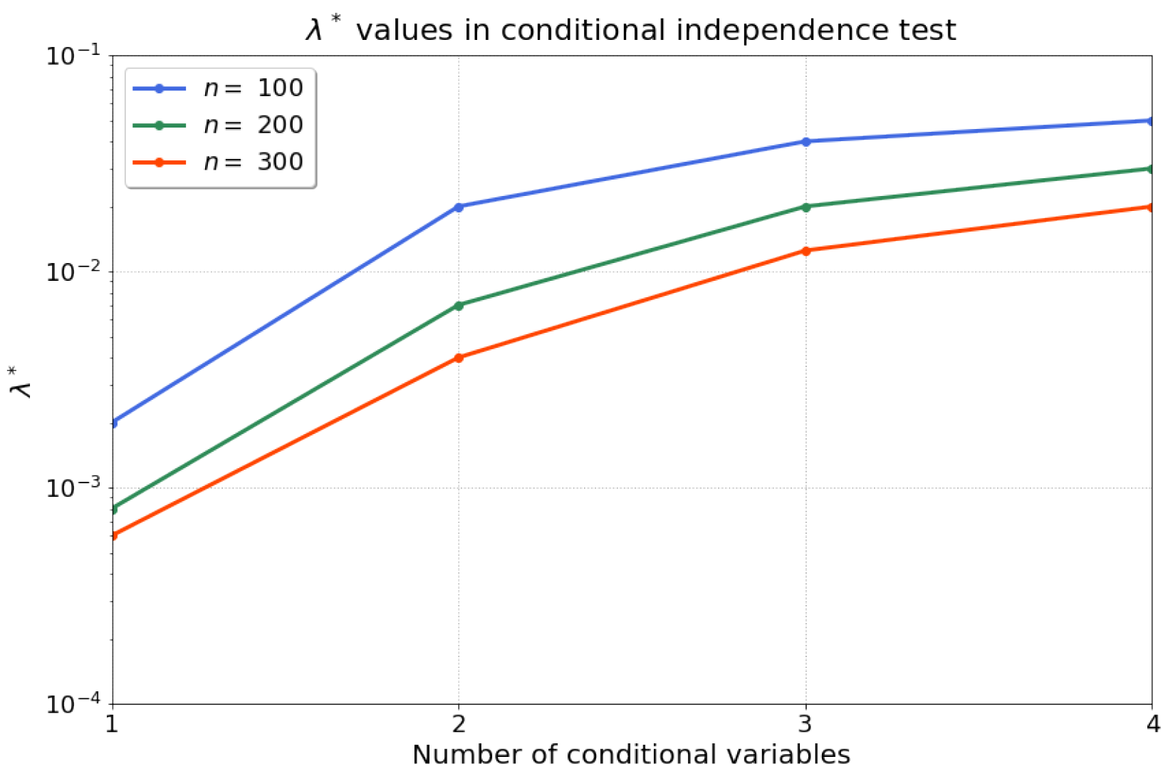
We then apply Algorithm 1 to compute the statistics for our conditional independence test. Firstly, we find that the optimised regularisation strength λ * is robust and reproducible for different random realisations with the same sample size and model parameters. Consequently, we search for one optimised λ * (line 1–18 in Algorithm 1) for each sample size, and fix this value for all 200 independent trials. Figure 2 summarises the results for λ * for n { 100 , 200 , 300 } samples after conducting a grid search over a range of 18 possible values 10 4 λ 10 1 , with P = 1000 permutations, and B = 100 rejection iterations. We find that the optimised λ * exhibits a saturation as the number of conditional variables (the dimension of the conditional set) is increased. Given that we perform a kernel ridge regression, a larger number of samples n should result in lower requirements for regularisation—which aligns with our observations of a decreasing λ * over the increase in number of samples n. Therefore, Algorithm 1 optimises the regularisation parameter λ * such that the evaluation rejection rate of the test is closest to the allowable false positive rate α = 0.05 .
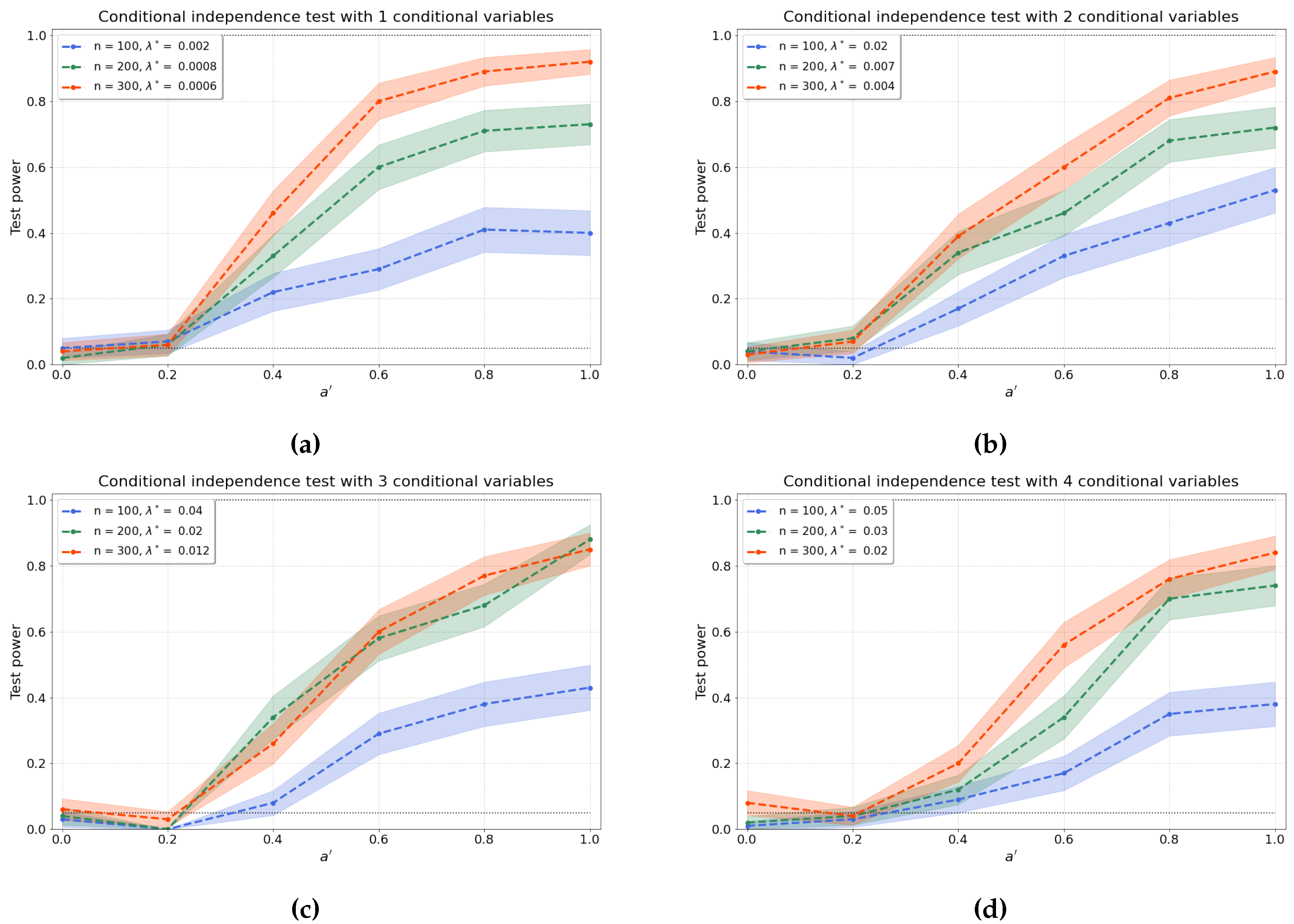
Figure 3a–d show the results of the conditional independence test for increasing dimension d of the conditional set (i.e., number of conditional variables). We find that the test power is well preserved as d increases through a concomitant increase of λ * that partly ameliorates the “curse of dimensionality” [47]. Furthermore, the values of the test power for a = 0 correspond to the type-I error rates.

4.2. Causal Structure Learning

We use the three independence tests evaluated numerically in Section 4.1 to learn different causal structures among function-valued random variables. We start with regression-based methods for the bivariate case X Y and extend to the multivariate case through regression-, constraint-based, and a combination of constraint- and regression-based causal structure learning approaches.

4.2.1. Synthetic Data

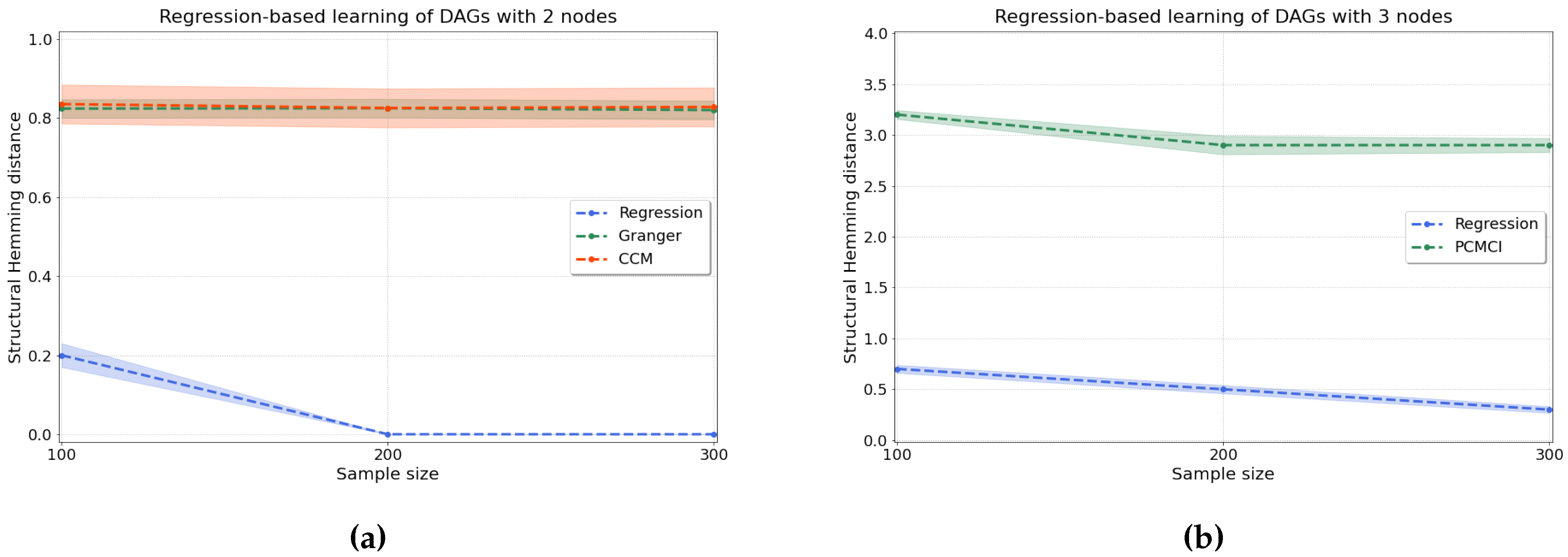
Regression-based causal discovery. The synthetic data for a bivariate system X Y is generated according to Equations (10)–(11) with a = 1 , and we measure the performance of the method by the structural Hemming distance (shd), whose definition can be found in Appendix E. As seen by the low value of the shd over 200 independent trials, Figure 4a shows that for this case our regression-based algorithm using resit outperforms two well-known algorithms for causal discovery: Granger-causality, which assumes linearity in the relationships [6], and ccm, which allows for non-linearity through a time-series embedding [7].
We also evaluate how the regression-based approach performs in a system of three variables where data are generated according to random dags with three nodes that entail historical non-linear dependence. The above methods (Granger, ccm) are commonly applied to sets with two variables only, hence we compare our method on a system with three variables to PC algorithm with momentary conditional independence (pcmci), an algorithm where each time point is represented as a node in a graph [48] from which we extract a directed graph for the variables. Figure 4b also shows improved performance of our regression-based algorithm, with a reduced shd. Details of the comparing methods are described in Appendix G.
Constraint-based causal discovery. The accuracy of our constraint-based approach is evaluated by computing three metrics: normalised shd ( s h d norm ), precision, and recall (see Appendix E for definitions). Figure 5 shows the accuracy of our algorithm when applied to d { 3 , 4 , 5 , 6 } variables.
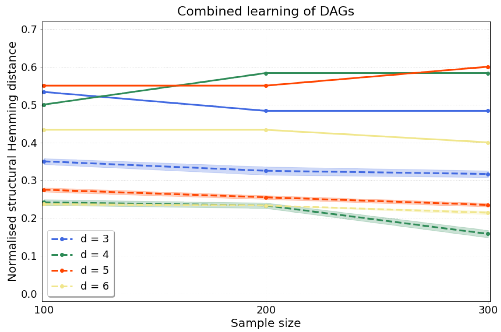
Combined approach. To be able to scale up our causal discovery techniques more efficiently to larger graphs, it is also possible to combine constraint- and regression-based causal learning, yielding dags. In this “combined” approach we start with a constraint-based step through which we learn cpdags by applying conditional independence tests to any two variables conditioned on any subset of the remaining d 2 variables and orient edges according to the Algorithm in Appendix F, which finds v-structures, applies Meek’s orientation rules and returns the Markov equivalence class. Often, the Markov equivalence class entails undirected edges, but we can then take a second step using a regression-based approach, under a different set of assumptions, to orient edges by applying resit. This two-step process finally yields a dag, i.e., every edge in the graph is oriented, in a more scalable manner than applying regression-based causal discovery directly. We then measure the accuracy of our approach computing the normalised shd (A4) as above. Figure 6 shows that our results for d = 3 , 4 , 5 , 6 variables compare favourably to pcmci.

4.2.2. Real-World Data

To showcase the application of our methods to real data, we return now to the motivating example on socio-economic indicators from the Introduction (Section 1). Sulemana and Kpienbaareh [2] tested for the causal direction between corruption and income inequality, as measured by the Control of Corruption index [8] and Gini coefficient [49], respectively. They applied Granger-causality with Wald- χ 2 tests, which statistically test against the null hypothesis that an assumed explanatory variable does not have an influence on other considered variables. Both variables, corruption and income inequality, were tested against being the explanatory variable (i.e., the cause) in their bivariate relationship. Their findings showed that income inequality as the explanatory variable results in a p-value of 0.079 , whereas corruption is more likely to be the cause with a p-value of 0.276 . Analysing the same data using ccm, which does not assume linearity, we also find the same cause-effect direction: 70.9 % of the sample pairs ( x i , y i ) validate corruption as the cause, against 29.7 % of pairs which detect the opposite direction. However, using our proposed regression-based kernel approach, which does not assume linearity or stationarity, we find the opposite result, i.e., the causal dependence of corruption on income inequality is statistically more likely (p = 0.0859 ) than the reverse direction (p = 0.0130 ).
Going beyond pairwise interactions, we have also applied our causal structure learning method to the set of World Governance Indicators (wgis) [8]. The wgis are a collection of six variables, which have been measured in 182 countries over 25 years from 1996 to 2020 (see Appendix H). We view the time-series of the countries as independent functional samples of each variable (so that n = 182 and the functional dimension is time), and we apply our methods as described above to establish the causal structure amongst the six wgis. In this case, we use the “combined” approach by successively applying our constraint- and regression-based causal structure learning methods. We first learn an undirected causal skeleton from the wgis (Figure 7a), and we find a triangle between Government Effectiveness (GE), Rule of Law (RL) and Control of Corruption (CC), and a separate link between Voice and Accountability (VA) and Regulatory Quality (RQ). We then orient these edges (Figure 7b) and find that Government Effectiveness (GE) causes both Rule of Law (RL) and Control of Corruption (CC), and Rule of Law (RL) causes Control of Corruption (CC). We also find that Voice and Accountability (VA) causes Regulatory Quality (RQ).

5. Discussion and Conclusion

We present a causal structure learning framework on functional data that utilises kernel-based independence tests to extend the applicability of the widely used regression- and constraint-based approaches. The foundation of the framework originates from the functional data analysis literature by interpreting any discrete-measured observations of a random variable as finite-dimensional realisations of functions.
Using synthetic data, we demonstrate that our regression-based approach significantly outperforms existing methods such as Granger-causality, ccm and pcmci when learning causal relationships between two and three variables. Further, we show that our conditional independence test, which is the cornerstone of the constraint-based causal discovery approach, achieves type-I error rates close to the acceptable false-positive rate α and high type-II error rates, even when the number of variables in the conditional set increases. Shah et al. [47] rightly state that any conditional independence test can suffer from an undesirable test size or low test power in finite samples, and our method is obviously no exception. However, Figure 3 demonstrates the counterbalance of the “curse of dimensionality” through the optimised regularisation strength λ * . Indeed, while with larger numbers of conditional variables, we would generally expect the test power to diminish, the optimisation of λ * offsets this reduction, resulting in no significant decrease in test power with a growing number of conditional variables. Although our proposed method is computationally expensive and significantly benefits from high sample sizes, a suitable regularisation strength could be chosen for large conditional sets in principle.
Furthermore, we demonstrate that constraint- and regression-based causal discovery methods can be combined to learn dags with large number of nodes, which would otherwise be computationally very expensive when relying on regression-based methods to yield dags. By comparing Figure 5a and Figure 6 we see however that it does not necessarily result in a lower shd. After learning the Markov equivalence class through the constraint-based approach, we apply regression with subsequent independence test (resit) to orient undirected edges in the “combined” approach. Here, mistakes in the orientation of undirected edges add 2 to the shd whereas an undirected edge only adds 1 to the shd.
The presented work contributes to opening the field of causal discovery to functional data. Beyond the results presented here, we believe that more research needs to be conducted to (i) increase the efficiency of the independence tests, meaning smaller sample sets can achieve higher test power; (ii) learn about upper bounds of the regularisation strength λ * with respect to the size of the sample and conditional sets; and (iii) make the computations in the conditional independence test less expensive.

Appendix A. Data

Appendix A.1. Fourier Basis Functions

Throughout our paper, we use the following Fourier basis functions:
ϕ 0 = 1 2 ϕ 2 m 1 , T ( s ) = sin ( 2 π m T s ) T 2 ϕ 2 m , T ( s ) = cos ( 2 π m T s ) T 2

Appendix A.2. Lower and Upper Bounds of β-Functions

Table A1. Lower and upper bounds of uniform distribution that define c 1 and c 2 in β .
Lower Bound Upper Bound
c 1 0.25 0.75
c 2 0.25 0.75
Figure A1. Function β ( s , t ) generated with random coefficients c 1 and c 2 as specified in Table A1.
Preprints 88915 g0a1

Appendix B. Proof of Theorem 1

Proof. 
All norms · and inner products · , · in this proof are taken with respect to the RKHS in which the normand and the arguments of the inner product reside in.
Denote by HSCIC ( X , Y , Z ) the true Hilbert-Schmidt conditional independence criterion between the random variables X and Y given Z , i.e.
HSCIC ( X , Y , Z ) = μ X Y | Z μ X | Z μ Y | Z ,
and denote by HSCIC ^ ( X , Y , Z , λ n ) the empirical estimate of HSCIC ( X , Y , Z ) based on samples, i.e.
HSCIC ^ ( X , Y , Z , λ n ) = μ ^ X Y | Z μ ^ X | Z μ ^ Y | Z ,
where μ ^ X Y | Z , μ ^ X | Z and μ ^ Y | Z are the empirical estimates of the conditional mean embeddings μ X Y | Z , μ X | Z and μ Y | Z obtained with the regularisation parameter λ n .
Note that by the reverse triangle inequality, followed by the ordinary triangle inequality, we have
HSCIC ( X , Y , Z ) HSCIC ^ ( X , Y , Z , λ n ) = μ X Y | Z μ X | Z μ Y | Z μ ^ X Y | Z μ ^ X | Z μ ^ Y | Z μ X Y | Z μ X | Z μ Y | Z μ ^ X Y | Z + μ ^ X | Z μ ^ Y | Z μ X Y | Z μ ^ X Y | Z + μ X | Z μ Y | Z μ ^ X | Z μ ^ Y | Z .
Here,
μ X | Z μ Y | Z μ ^ X | Z μ ^ Y | Z 2 = μ X | Z μ Y | Z , μ X | Z μ Y | Z 2 μ X | Z μ Y | Z , μ ^ X | Z μ ^ Y | Z + μ ^ X | Z μ ^ Y | Z , μ ^ X | Z μ ^ Y | Z = μ X | Z , μ X | Z μ Y | Z , μ Y | Z 2 μ X | Z , μ ^ X | Z μ Y | Z , μ ^ Y | Z + μ ^ X | Z , μ ^ X | Z μ ^ Y | Z , μ ^ Y | Z = μ X | Z , μ X | Z μ Y | Z , μ Y | Z 2 μ X | Z , μ X | Z μ Y | Z , μ ^ Y | Z + 2 μ X | Z , μ X | Z μ ^ X | Z μ Y | Z , μ ^ Y | Z + μ X | Z , μ X | Z μ ^ Y | Z , μ ^ Y | Z + μ ^ X | Z μ X | Z , μ ^ X | Z + μ X | Z μ ^ Y | Z , μ ^ Y | Z = μ X | Z , μ X | Z μ Y | Z μ ^ Y | Z 2 + 2 μ X | Z , μ X | Z μ ^ X | Z μ Y | Z , μ ^ Y | Z + μ ^ X | Z μ X | Z , μ ^ X | Z + μ X | Z μ ^ Y | Z , μ ^ Y | Z μ X | Z 2 μ Y | Z μ ^ Y | Z 2 + μ X | Z μ ^ X | Z 2 μ X | Z μ Y | Z , μ ^ Y | Z + μ ^ X | Z + μ X | Z μ ^ Y | Z ,
where we used the Cauchy-Schwarz inequality in the last inequality. We note that Theorem 4.4 Park and Muandet [17] ensures that each of μ X Y | Z μ ^ X Y | Z , μ Y | Z μ ^ Y | Z and μ X | Z μ ^ X | Z converge to 0 in probability, hence HSCIC ^ ( X , Y , Z , λ n ) HSCIC ( X , Y , Z ) in probability with respect to the L 2 -norm.
Now we show that the empirical average of the empirical HSCIC converges to the population integral of the population HSCIC. Writing HSCIC ^ as a shorthand for HSCIC ^ ( X , Y , Z , λ n ) , we see that
1 n i = 1 n HSCIC ^ ( z i ) HSCIC ( z ) d P ( z ) 1 n i = 1 n HSCIC ^ ( z i ) HSCIC ^ ( z ) d P ( z ) + HSCIC ^ ( z ) d P ( z ) HSCIC ( z ) d P ( z ) sup f F 1 n i = 1 n f ( z i ) f ( z ) d P ( z ) + HSCIC ^ ( z ) d P ( z ) HSCIC ( z ) d P ( z ) .
Here, the first term converges to 0 thanks to the uniform law of large numbers over the function class F in which the empirical estimation of HSCIC ^ is carried out, and the second term converges to 0 as shown above.
Now, by Park and Muandet [17, Theorem 5.4], since our kernel k 1 k 2 is characteristic, we have that HSCIC ( X , Y , Z ) is the identically zero function if and only if X Y Z . Hence, if the alternative hypothesis H 1 holds, we have
HSCIC ( z ) d P ( z ) > 0 .
See that, for any r > 0 , we have
lim n P 1 n i = 1 n HSCIC ^ ( z i ) r = 1 lim n P 1 n i = 1 n HSCIC ^ ( z i ) < r = 1 lim n P 1 n i = 1 n HSCIC ^ ( z i ) r n < 0 = 1 lim n P HSCIC ( z ) d P ( z ) < 0 = 1 ,
where we used Portmanteau’s theorem [50, p.6, Lemma 2.2] to get from the second line to the third, using the convergence of 1 n i = 1 n HSCIC ^ ( z i ) to HSCIC ( z ) d P ( z ) shown above. Hence, our test is consistent.    □

Appendix C. Supplementary Information about Computational Complexity

When applying the regression-based causal discovery approach, one needs to iterate over all possible candidate dags. Each candidate dag is one potential configuration of the causal graph and needs to be evaluated against the possibility that it generated the observed data. The total number of candidate dags κ d of a graph with d nodes is given by
κ d = i = 1 d ( 1 ) i + 1 d i 2 i ( d i ) κ d i .
When utilising the constraint-based approach, one needs to exhaustively test for conditional independence between any two nodes of the graph given any possible subset of the remaining nodes. Including the empty conditional set, this results in 2 d 2 conditional independence tests for every pair of nodes in the graph. Then, the total number of conditional independence tests η d , that is, the pairs of nodes in a graph of d nodes multiplied by the number of conditional independence tests is given by
η d = d 2 2 d 2 .

Appendix D. Supplementary Definitions

Appendix D.1. D-Separation

If X , Y and Z are three pairwise disjoint (sets of) nodes in a dagG, then Z d-separates X from Y in G if Z blocks every possible path between (any node in) X and (any node in) Y in G [34, § 1.2.3]. We then write X G Y | Z . The symbol G is commonly used to denote d-separation.

Appendix D.2. Faithfulness Assumption

If two random variables are (conditionally) independent in the observed distribution P , then they are d-separated in the underlying causal graph G [Definition 6.33 [36].

Appendix D.3. Causal Markov Assumption

The distribution P X Y Z is Markov with respect to a dagG if X G Y | Z X Y | Z for all disjoint (sets of) nodes X , Y , Z , where G denotes d-separation [Definition 6.21 [36].

Appendix E. Definitions of Metrics

Appendix E.1. shd

For two graphs, G 1 and G 2 , shd is the sum of the element-wise absolute differences between the adjacency matrices A 1 and A 2 of G 1 and G 2 , respectively.
SHD = i | A 1 i A 2 i | ,
where we iterate over each element i in the adjacency matrices. Thus, when a learnt causal graph G 1 including an edge, e.g., X Y is oriented opposite to the corresponding edge in the true graph G 2 , meaning X Y is true, we add 2 to the shd score (“double penalty”). Note that others [e.g., 51] only penalise by 1 for a learnt edge being directed opposite to the true edge.

Appendix E.2. Normalised shd

We normalise the shd by the number of possible directed edges in a graph of size d, thus allowing comparison across graphs with different number of nodes.
SHD norm = s h d d ( d 1 ) .

Appendix E.3. Precision

We define the total number of edges in a learnt graph G 1 as the sum of truly and falsely learnt edges, e = e t + e f . The truly learnt edges are the edges that correspond to the zero elements in the matrix containing the element-wise differences between the learnt A 1 and the true A 2 . In contrast, the falsely learnt edges are the non-zero elements. The total number of truly and falsely learnt edges are e t and e f , respectively. Precision is the proportion of correctly oriented edges e t in a learnt graph G 1 in comparison to a true graph G 2 out of all learnt edges e in G 1 .
Precision = e t e

Appendix E.4. Recall

We separate between oriented and oriented edges, e o and e u , respectively, which can again be summed up to the total number of edges, e = e o + e u . Recall is the fraction of edges in the cpdag that are oriented:
Recall = e o e .

Appendix F. Meek’s Orientation Rules, the SGS and the PC Algorithms
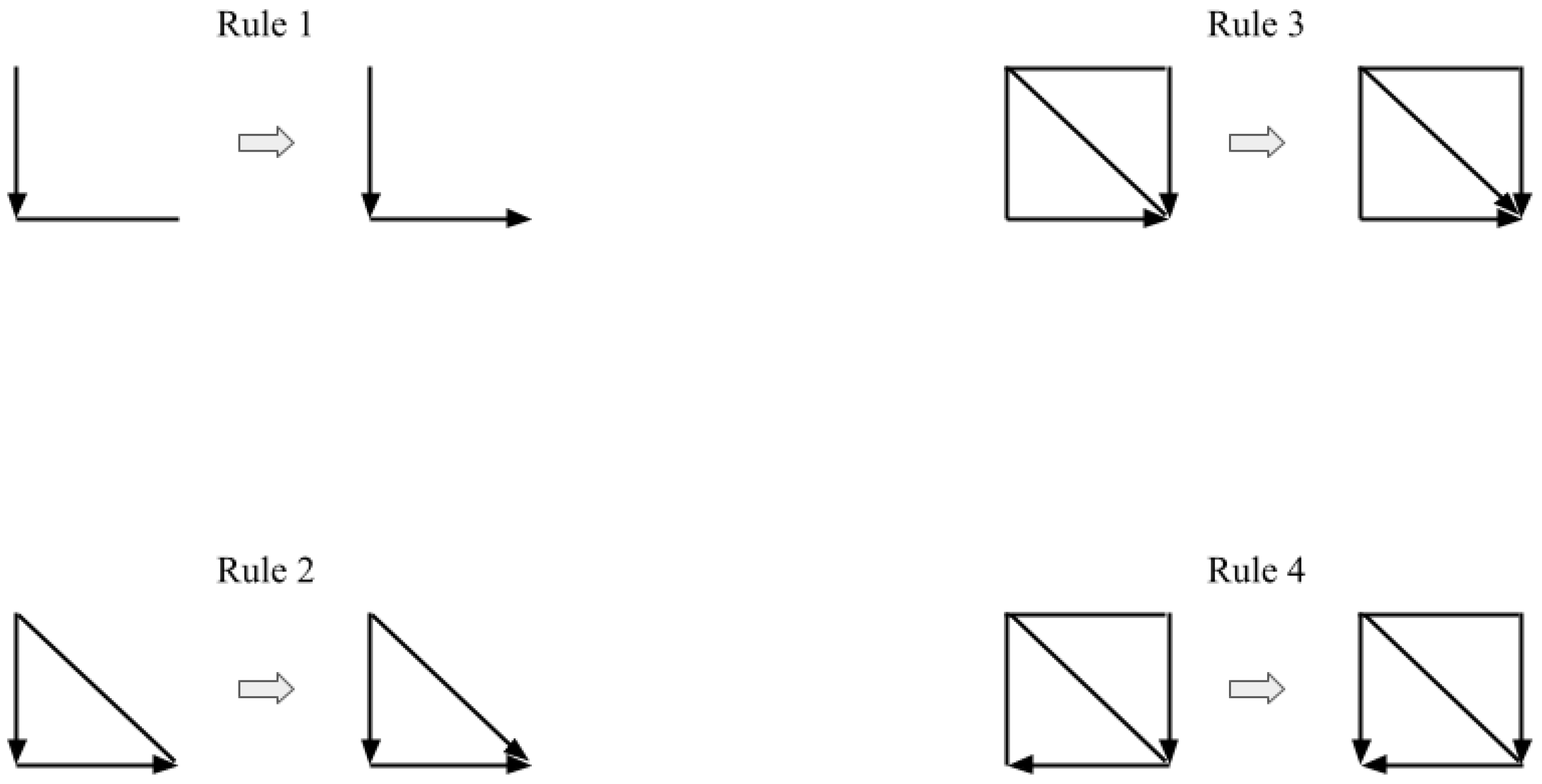
In Figure A2, a node is placed at each end of the edges. Rule 1 states that if one directed edge (here the vertical edge) points towards another undirected edge (the horizontal edge) that is not further connected to any other edges, the undirected edge must point in the same direction as the adjacent edge, because the three vertices would otherwise form a v-structure (which are only formed with conditional dependence). Rule 2, in contrast, points the undirected edge in both adjacent vertices’ direction because it would violate the acyclicity of a dag otherwise. Rule 3 and 4 avoid new v-structures which would come into existence by applying Rule 2 twice if the oriented edges pointed in the opposite direction. These new v-structures would be in the left top corners of the rectangles.
Figure A2. Meek rules to orient edges that remain in the graph after conditional independence tests and edges are oriented based on detected colliders. Proofs that edges cannot be oriented in the opposite direction without violating the acyclicity of the graph and found conditional independencies are given in Meek [44].
Preprints 88915 g0a2
Based on Meek’s orientation rules, the SGS algorithm tests each pair of variables as follows [13, § 5.4.1]:
  • Form the complete undirected graph G from the set of vertices (or nodes) V .
  • For each pair of vertices X and Y, if there exists a subset S of V { X , Y } such that X and Y are d-separated, i.e., conditionally independent (causal Markov condition), given Z, remove the edge between X and Y from G.
  • Let K be the undirected graph resulting from the previous step 2. For each triple of vertices X, Y, and Z such that the pair X and Y and the pair Y and Z are each adjacent in K (written as X Y Z ) but the pair X and Z are not adjacent in K, orient X Y Z as X Y Z if and only if there is no subset S of Y that d-separates X and Z.
  • Repeat the following steps until no more edges can be oriented:
    (a)
    If X Y , Y and Z are adjacent, X and Z are not adjacent, and there is no arrowhead of other vertices at Y, then orient Y Z as Y Z (Rule 1 of Meek’s orientation rules).
    (b)
    If there is a directed path over some other vertices from X to Y, and an edge between X and Y, then orient X Y as X Y (Rule 2 of Meek’s orientation rules).
The large computational cost of applying the SGS algorithm (especially step 2) to data, due to the large number of combinations of variables as the potential conditional sets, opened the door for computationally more efficient methods. The PC algorithm [13, § 5.4.2] is amongst the most popular alternatives and minimises the computational cost by searching for conditional independence in a structured manner, as opposed to step 2 of the SGS algorithm that iterates over all possible conditional subsets to any two variables A and B. Starting again with a fully connected undirected graph, the PC algorithm begins by testing for marginal independence between any two variables A and B and deletes the edge connecting A and B, A B , if A B . Then, it proceeds with testing for A B | C and erases A B if one conditional variable C is found that makes A and B independent given C. Afterwards, the conditional set is extended to two variables, { C , D } , and the edge A B is deleted if this conditional set makes A and B independent. The conditional set is extended, round after round, until no more conditional independencies are found, resulting in the sparsified graph K. Step 3 and 4 are then pursued as in the SGS algorithm.

Appendix G. Comparison Methods

Appendix G.1. Granger-Causality

We implement Granger-causality through software provided by Seabold and Perktold [52] and define the optimal lag as the first local minimum in the mutual information function over measurement points. Given that Granger-causality is applied to a pair of samples, ( x i , y i ) , we iterate over every pair and determine the percentage of pairs that result in X Y against X Y .

Appendix G.2. ccm

We implement ccm through software provided by 53 and define the optimal lag as for Granger-causality. The embedding dimensionality is determined by a false nearest neighbour method [53]. As with Granger-causality, ccm is also applied to a pair of samples, ( x i , y i ) . We take the same summarising approach and iterate over every pair and determine the percentage of of pairs that result in X Y against X Y .

Appendix G.3. pcmci

Runge et al. [48] proposed pcmci, a method that produces time-series graphs where each node represents a variable at a certain state in time. When applying the method in our experiments, we estimate the maximum possible lag as the average of the first local minimum of mutual information of all considered data series. Then, we test for the presence of an edge by applying distance correlation-based independence tests [54] between the residuals of X and Y that remain after regressing out the influence of the remaining nodes in the graph through Gaussian processes. The distance correlation coefficients of the significant edges between two variables are summed up to measure the prevalence of a causal direction of edges connecting these two variables. The causal direction with the greater sum is then considered to be the directed edge, and assessed against the edge between the same two variables in the true dag.

Appendix H. World Governance Indicators

In Figure 7, we abbreviate the variables according to the official names that are mentioned in Table A2. The Descriptions are taken from the Documentation on https://info.worldbank.org/governance/wgi/. The data set consists of six variables (normalised to a range from 0 to 100), of which each is a summary of multiple indicators measured over 25 years from 1996 to 2020 in 182 countries. The methodology about how the summarising measure is calculated can be found in Kaufmann et al. [8, §4].
Table A2. Abbreviations together with official names and descriptions of the variables in the data set of the World Governance Indicators.
Abbreviation Official Name Description
VA Voice and Accountability Voice and accountability captures perceptions of the extent to which a country’s citizens are able to participate in selecting their government, as well as freedom of expression, freedom of association, and a free media.
PS Political Stability and No Violence Political Stability and Absence of Violence/Terrorism measures perceptions of the likelihood of political instability and/or politically-motivated violence, including terrorism.
GE Government Effectiveness Government effectiveness captures perceptions of the quality of public services, the quality of the civil service and the degree of its independence from political pressures, the quality of policy formulation and implementation, and the credibility of the government’s commitment to such policies.
RQ Regulatory Quality Regulatory quality captures perceptions of the ability of the government to formulate and implement sound policies and regulations that permit and promote private sector development.
RL Rule of Law Rule of law captures perceptions of the extent to which agents have confidence in and abide by the rules of society, and in particular the quality of contract enforcement, property rights, the police, and the courts, as well as the likelihood of crime and violence.
CC Control of Corruption Control of corruption captures perceptions of the extent to which public power is exercised for private gain, including both petty and grand forms of corruption, as well as "capture" of the state by elites and private interests.
  

References

  1. Runge, J.; Bathiany, S.; Bollt, E.; Camps-Valls, G.; Coumou, D.; Deyle, E.; Glymour, C.; Kretschmer, M.; Mahecha, M.D.; Muñoz-Marí, J.; et al. Inferring causation from time series in Earth system sciences. Nature communications 2019, 10, 1–13. [Google Scholar] [CrossRef]
  2. Sulemana, I.; Kpienbaareh, D. An empirical examination of the relationship between income inequality and corruption in Africa. Economic Analysis and Policy 2018, 60, 27–42. [Google Scholar] [CrossRef]
  3. Finkle, J.D.; Wu, J.J.; Bagheri, N. Windowed granger causal inference strategy improves discovery of gene regulatory networks. Proceedings of the National Academy of Sciences 2018, 115, 2252–2257. [Google Scholar] [CrossRef]
  4. Glymour, C.; Zhang, K.; Spirtes, P. Review of causal discovery methods based on graphical models. Frontiers in genetics 2019, 10, 524. [Google Scholar] [CrossRef]
  5. Ramsay, J.O.J.O. Functional Data Analysis, 2nd ed.; Springer Series in Statistics; Springer: New York, NY, USA, 2005. [Google Scholar]
  6. Granger, C.W. Investigating causal relations by econometric models and cross-spectral methods. Econom. J. Econom. Soc. 1969, 424–438. [Google Scholar] [CrossRef]
  7. Sugihara, G.; May, R.; Ye, H.; Hsieh, C.h.; Deyle, E.; Fogarty, M.; Munch, S. Detecting causality in complex ecosystems. science 2012, 338, 496–500. [Google Scholar] [CrossRef]
  8. Kaufmann, D.; Kraay, A.; Mastruzzi, M. The worldwide governance indicators: Methodology and analytical issues1. Hague journal on the rule of law 2011, 3, 220–246. [Google Scholar] [CrossRef]
  9. World Bank. Gini index. 2022. [Google Scholar]
  10. Jong-Sung, Y.; Khagram, S. A comparative study of inequality and corruption. American sociological review 2005, 70, 136–157. [Google Scholar] [CrossRef]
  11. Alesina, A.; Angeletos, G.M. Corruption, inequality, and fairness. Journal of Monetary Economics 2005, 52, 1227–1244. [Google Scholar] [CrossRef]
  12. Dobson, S.; Ramlogan-Dobson, C. Is there a trade-off between income inequality and corruption? Evidence from Latin America. Economics letters 2010, 107, 102–104. [Google Scholar] [CrossRef]
  13. Spirtes, P.; Glymour, C.N.; Scheines, R.; Heckerman, D. Causation, Prediction, and Search. MIT Press, 2000. [Google Scholar]
  14. Peters, J.; Mooij, J.M.; Janzing, D.; Schölkopf, B. Causal discovery with continuous additive noise models. The Journal of Machine Learning Research 2014, 15, 2009–2053. [Google Scholar]
  15. Muandet, K.; Fukumizu, K.; Sriperumbudur, B.; Schölkopf, B.; et al. Kernel mean embedding of distributions: A review and beyond. Foundations and Trends in Machine Learning 2017, 10, 1–141. [Google Scholar] [CrossRef]
  16. Wynne, G.; Duncan, A.B. A kernel two-sample test for functional data. Journal of Machine Learning Research 2022, 23, 1–51. [Google Scholar]
  17. Park, J.; Muandet, K. A measure-theoretic approach to kernel conditional mean embeddings. arXiv 2020, arXiv:2002.03689 2020. [Google Scholar]
  18. Berrett, T.B.; Wang, Y.; Barber, R.F.; Samworth, R.J. The conditional permutation test for independence while controlling for confounders. Journal of the Royal Statistical Society: Series B (Statistical Methodology) 2020, 82, 175–197. [Google Scholar] [CrossRef]
  19. Malfait, N.; Ramsay, J.O. The historical functional linear model. Canadian Journal of Statistics 2003, 31, 115–128. [Google Scholar] [CrossRef]
  20. Pfister, N.; Bühlmann, P.; Schölkopf, B.; Peters, J. Kernel-based tests for joint independence. Journal of the Royal Statistical Society: Series B (Statistical Methodology) 2018, 80, 5–31. [Google Scholar] [CrossRef]
  21. Ramos-Carreño, C.; Suárez, A.; Torrecilla, J.L.; Carbajo Berrocal, M.; Marcos Manchón, P.; Pérez Manso, P.; Hernando Bernabé, A.; García Fernández, D.; Hong, Y.; Rodríguez-Ponga Eyriès, P.M.; et al. GAA-UAM/scikit-fda: Version 0.7.1. 2022. [Google Scholar] [CrossRef]
  22. Squires, C. causaldag: creation, manipulation, and learning of causal models. 2018. [Google Scholar]
  23. Girard, O.; Lattier, G.; Micallef, J.P.; Millet, G.P. Changes in exercise characteristics, maximal voluntary contraction, and explosive strength during prolonged tennis playing. British journal of sports medicine 2006, 40, 521–526. [Google Scholar] [CrossRef] [PubMed]
  24. Zhu, Y.; Kuhn, T.; Mayo, P.; Hinds, W.C. Comparison of daytime and nighttime concentration profiles and size distributions of ultrafine particles near a major highway. Environmental science & technology 2006, 40, 2531–2536. [Google Scholar]
  25. Ramsay, J.; Hooker, G. Dynamic Data Analysis. Springer, 2017. [Google Scholar]
  26. Fukumizu, K.; Gretton, A.; Sun, X.; Schölkopf, B. Kernel Measures of Conditional Dependence. In Proceedings of the Advances in Neural Information Processing Systems; Platt, J.C., Koller, D., Singer, Y., Roweis, S., Eds.; Red Hook, NY, USA, 2008; Volume 20, pp. 489–496. [Google Scholar]
  27. Gretton, A.; Fukumizu, K.; Teo, C.H.; Song, L.; Schölkopf, B.; Smola, A.J. A kernel statistical test of independence. In Proceedings of the Advances in neural information processing systems; 2008; pp. 585–592. [Google Scholar]
  28. Zhang, K.; Peters, J.; Janzing, D.; Schölkopf, B. Kernel-based conditional independence test and application in causal discovery. arXiv 2012, arXiv:1202.3775 2012. [Google Scholar]
  29. Lai, T.; Zhang, Z.; Wang, Y.; Kong, L. Testing independence of functional variables by angle covariance. Journal of Multivariate Analysis 2021, 182, 104711. [Google Scholar] [CrossRef]
  30. Górecki, T.; Krzyśko, M.; Wołyński, W. Independence test and canonical correlation analysis based on the alignment between kernel matrices for multivariate functional data. Artificial Intelligence Review 2020, 53, 475–499. [Google Scholar] [CrossRef]
  31. Doran, G.; Muandet, K.; Zhang, K.; Schölkopf, B. A Permutation-Based Kernel Conditional Independence Test. In Proceedings of the UAI. Citeseer; 2014; pp. 132–141. [Google Scholar]
  32. Gretton, A.; Borgwardt, K.M.; Rasch, M.J.; Schölkopf, B.; Smola, A. A kernel two-sample test. The Journal of Machine Learning Research 2012, 13, 723–773. [Google Scholar]
  33. Lee, S.; Honavar, V.G. Self-discrepancy conditional independence test. In Proceedings of the Uncertainty in artificial intelligence; 2017; Voulme 33. [Google Scholar]
  34. Pearl, J. Causality; Cambridge University Press, 2009. [Google Scholar]
  35. Mooij, J.M.; Peters, J.; Janzing, D.; Zscheischler, J.; Schölkopf, B. Distinguishing cause from effect using observational data: methods and benchmarks. The Journal of Machine Learning Research 2016, 17, 1103–1204. [Google Scholar]
  36. Peters, J.; Janzing, D.; Schölkopf, B. Elements of Causal Inference; The MIT Press, 2017. [Google Scholar]
  37. Schölkopf, B.; von Kügelgen, J. From statistical to causal learning. arXiv 2022, arXiv:2204.00607 2022. [Google Scholar]
  38. Squires, C.; Uhler, C. Causal structure learning: a combinatorial perspective. In Foundations of Computational Mathematics; 2022; pp. 1–35. [Google Scholar]
  39. Vowels, M.J.; Camgoz, N.C.; Bowden, R. D’ya like dags? a survey on structure learning and causal discovery. ACM Computing Surveys 2022, 55, 1–36. [Google Scholar] [CrossRef]
  40. Chickering, D.M. Optimal structure identification with greedy search. Journal of machine learning research 2002, 3, 507–554. [Google Scholar]
  41. Shimizu, S.; Hoyer, P.O.; Hyvärinen, A.; Kerminen, A.; Jordan, M. A linear non-Gaussian acyclic model for causal discovery. Journal of Machine Learning Research 2006, 7. [Google Scholar]
  42. Hoyer, P.; Janzing, D.; Mooij, J.M.; Peters, J.; Schölkopf, B. Nonlinear causal discovery with additive noise models. Advances in neural information processing systems 2008, 21. [Google Scholar]
  43. Szabó, Z.; Sriperumbudur, B.K. Characteristic and Universal Tensor Product Kernels. J. Mach. Learn. Res. 2017, 18, 1–29. [Google Scholar]
  44. Meek, C. Complete Orientation Rules for Patterns; Carnegie Mellon [Department of Philosophy], 1995. [Google Scholar]
  45. Peters, J.; Mooij, J.; Janzing, D.; Schölkopf, B. Identifiability of causal graphs using functional models. arXiv 2012, arXiv:1202.3757 2012. [Google Scholar]
  46. Bühlmann, P.; Peters, J.; Ernest, J. CAM: Causal additive models, high-dimensional order search and penalized regression. 2014. [Google Scholar]
  47. Shah, R.D.; Peters, J.; et al. The hardness of conditional independence testing and the generalised covariance measure. Annals of Statistics 2020, 48, 1514–1538. [Google Scholar] [CrossRef]
  48. Runge, J.; Nowack, P.; Kretschmer, M.; Flaxman, S.; Sejdinovic, D. Detecting and quantifying causal associations in large nonlinear time series datasets. Science advances 2019, 5. [Google Scholar] [CrossRef]
  49. Gini, C. On the measure of concentration with special reference to income and statistics. Colorado College Publication, General Series 1936, 208, 73–79. [Google Scholar]
  50. Van der Vaart, A.W. Asymptotic Statistics; Cambridge University Press, 2000; Volume 3. [Google Scholar]
  51. Peters, J.; Bühlmann, P. Structural intervention distance for evaluating causal graphs. Neural computation 2015, 27, 771–799. [Google Scholar] [CrossRef] [PubMed]
  52. Seabold, S.; Perktold, J. statsmodels: Econometric and statistical modeling with python. In Proceedings of the 9th Python in Science Conference; 2010. [Google Scholar]
  53. Munch, E.; Khasawneh, F.; Myers, A.; Yesilli, M.; Tymochko, S.; Barnes, D.; Guzel, I.; Chumley, M. teaspoon: Topological Signal Processing in Python. 2022. [Google Scholar]
  54. Székely, G.J.; Rizzo, M.L.; Bakirov, N.K. Measuring and testing dependence by correlation of distances. 2007. [Google Scholar]
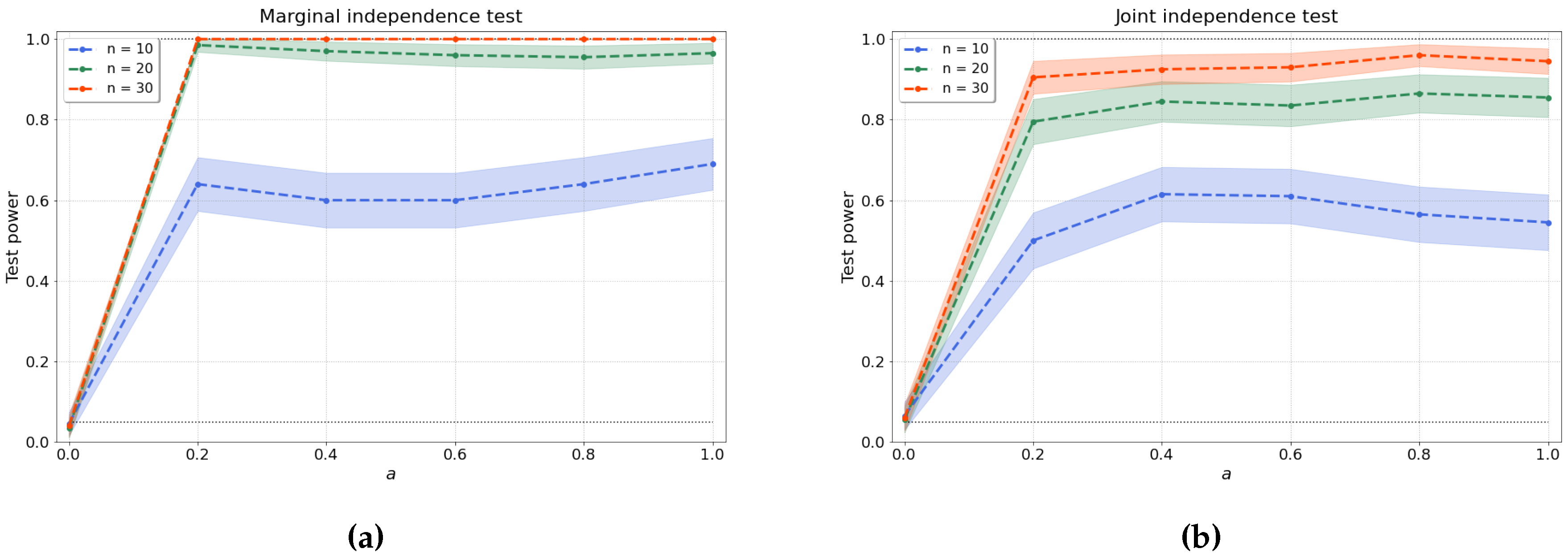
Figure 1. (a) Bivariate and (b) joint independence tests over various values of the dependence factor a and sample size n. The joint independence test is conducted with d = 4 variables.
Preprints 88915 g001
Figure 2. The optimised λ * for increasing dimension d of the evaluated size of the conditional set and different sample sizes n { 100 , 200 , 300 } .
Preprints 88915 g002
Figure 3. The test power of the conditional independence tests over various values for a and sample sizes n, from (a) 1 to (d) 4 conditional variables. The regularisation parameter λ * is given in the legend.
Preprints 88915 g003
Figure 4. Regression-based causal discovery using kernel-based joint independence tests among residuals with (a) two and (b) three variables. In the case of two variables (a), we compare to Granger-causality and ccm. In the case of three variables (b), we used pcmci to produce comparable results. Our method significantly outperforms both Granger-causality and ccm in the bivariate setting, with just a few mistakes made for low sample numbers ( n = 100 ) and no mistakes for higher sample sizes. For three variables, our method is substantially more accurate than pcmci, with an average shd of 0.3 at n = 300 versus 2.9 for pcmci. The accuracy is measured in terms of the structural Hemming distance (shd).
Preprints 88915 g004
Figure 5. Constraint-based causal structure learning experiments. From left to right, we compute (a) the normalised shd, (b) precision and (c) recall over d { 3 , 4 , 5 , 6 } variables and n { 100 , 200 , 300 } samples with a = 1 as the factor of the dependence between any two variables in the data that are connected by an edge in the true dag.
Preprints 88915 g005
Figure 6. Causal structure learning with the “combined” approach, where we first apply the constraint-based method to find the Markov equivalence class, followed by the regression-based method to orient the undirected edges of the Markov equivalence class. Our results (dashed lines) are compared to results obtained from pcmci (solid lines), as described in Appendix G. We compute the normalised shd over d { 3 , 4 , 5 , 6 } variables and n { 100 , 200 , 300 } samples with a = 1 .
Preprints 88915 g006
Figure 7. Undirected (a) and directed (b) causal networks on the World Governance Indicators data set to evaluate the results of the constraint-based approach alone (a) and the subsequent regression-based approach (b). The labels are abbreviations of the official names: Voice and Accountability (VA), Political Stability (PS), Government Effectiveness (GE), Regulatory Quality (RQ), Rule of Law (RL), and Control of Corruption (CC) (see Appendix H).
Preprints 88915 g007
Disclaimer/Publisher’s Note: The statements, opinions and data contained in all publications are solely those of the individual author(s) and contributor(s) and not of MDPI and/or the editor(s). MDPI and/or the editor(s) disclaim responsibility for any injury to people or property resulting from any ideas, methods, instructions or products referred to in the content.
Copyright: This open access article is published under a Creative Commons CC BY 4.0 license, which permit the free download, distribution, and reuse, provided that the author and preprint are cited in any reuse.
Prerpints.org logo

Preprints.org is a free preprint server supported by MDPI in Basel, Switzerland.

Subscribe

Disclaimer

Terms of Use

Privacy Policy

Privacy Settings

© 2025 MDPI (Basel, Switzerland) unless otherwise stated