
Submitted:
19 May 2025
Posted:
19 May 2025
You are already at the latest version
Abstract
We present an analytical framework for describing light propagation in infinite waveguide arrays, incorporating a generalized long-range coupling to achieve a more realistic model. We demonstrate that the resulting solution can be expressed in terms of generalized Bessel-like functions. Additionally, by applying the concept of eigenstates, we borrow from quantum mechanics a basis given in terms of phase states that allows the analysis of the transition from the discrete to the continuum limit, obtaining a relationship between the field amplitudes and the Fourier series coefficients of a given function. We apply our findings to different coupling functions, providing new insights into the propagation dynamics of these systems.
Keywords:
waveguide arrays
; propagation
; phase states
; generalized bessel function
1. Introduction
The interaction between particles mediated by a field cannot be entirely captured by a distance action, which offers only an approximate description. A more refined approach considers two-body, three-body, and higher-order m-body interactions as successive corrections to this approximation. The relative magnitudes of these interaction terms can be systematically analyzed for different types of classical and quantum fields, such as the electromagnetic [1]. Quantum long-range systems have recently attracted significant interest, driven not only by the need to explore the fundamental physics of nonlocal interactions and their influence on the balance between local and long-distance properties but also by their potential in quantum technology applications. Their collective nature improves the distribution of entanglement and gives rise to unique dynamical scaling effects, as they facilitate the generation of highly entangled or correlated dynamical states [2,3,4]. Nevertheless, the exponential growth of the Hilbert space with system size makes it inherently difficult to efficiently simulate the quantum physics of an interacting many-body system using classical computers. Recognizing this limitation, Feynman proposed a controllable quantum device as an alternative, allowing for an efficient study of the dynamics of another quantum system, and since then, quantum simulation has emerged as an independent and rapidly evolving field of research [5]. Significant progress in experimental techniques and theoretical frameworks has driven intensive research in quantum simulation across diverse physical platforms. Among them, atomic, molecular and optical systems; ranging from trapped ions and cold atoms to arrays of evanescently coupled waveguides, have garnered significant attention [6,7,8,9,10,11,12,13].
Coupled optical waveguide arrays and periodic photonic lattices have been the focus of intense research because of the diverse physical phenomena that emerge from the interplay of discreteness, periodicity, nonlinearity, and boundary effects. Beyond their fundamental interest, these structures enable the control and manipulation of light propagation, facilitating the observation of phenomena such as Bloch oscillations, Anderson localization, and quantum walks, among others [14,15,16,17,18,19,20,21]. However, in these structures, coupling is generally assumed to occur only between nearest-neighbor waveguides, while interactions with more distant waveguides are typically neglected under the assumption that the coupling strength decays exponentially with distance. However, second-order couplings can play a significant role in the structure of the waveguide array, as seen in the two-dimensional zigzag waveguide lattice, where an exact solution can be found [22,23,24]. Moreover, higher-order couplings have been observed in circular and helical waveguide arrays [25,26,27], and their advantages have been extensively documented in the literature, particularly in applications such as quantum state modeling, Bloch oscillations, and photon-number correlations [28,29,30,31,32,33].
The structure of this article is as follows. Section 2 begins by analyzing an infinite waveguide array where interactions extend beyond nearest neighbors. By employing phase states, we derive an exact solution, which closely relates to the case of first-neighbor interactions in an infinite array. In Section 3, we introduce an alternative approach based on operational methods to solve the same system. In Section 4, we extend the waveguide-array interactions to an infinite number of neighbors, which allows the approximation of the discrete solutions as continuous functions and compute the evolution of the amplitude for different coupling functions. Finally, in Section 5, we summarize our findings and present concluding remarks.
2. Interaction with N Neighbors
In coupled mode theory, the propagation of an optical field through a waveguide array with long-range evanescent coupling without frontiers is governed by the following set of coupled first order ordinary differential equations
In this context, z represents the propagation distance, while denotes a set of real and nonnegative coupling constants. The index j ranges across all integers from to ∞.
This framework can be viewed also as the problem of solving the Schrödinger-like equation with Hamiltonian
where the operators and are the generalized London operators defined as [34,35],
which in the infinite Hilbert space commute. The sum in the Hamiltonian (2) may define either a polynomial for finite N or a function in the limit .
If we denote the solution of the Schrödinger-type equation associated with the Hamiltonian (2) as , it is easy to demonstrate that the solutions of system (1) are given by . Using operational methods, we solve the Schrödinger-like equation derived from the Hamiltonian (2) and subsequently obtain the solution for the infinite system in (1). Considering an arbitrary initial condition , the formal solution of the Schrödinger-like equation is expressed as ; to solve this equation, we introduce the phase states [36,37] defined as
in such a way that it is easy to prove , and . The phase states defined above form a complete basis, so the unity operator may be written as , and the initial condition may be given in terms of phase states as
with .
Given that and commute, the propagation of an arbitrary field can be formulated applying the operators and carrying out some algebraic steps, we get
and in order to find the amplitudes that are the solutions of the system (1) we project the above expression over the state and use the fact that , obtaining
We take now as initial condition , where m is an integer, and thus , which substituted in Eq. (7) gives
although the integral above can be efficiently solved using numerical methods to determine the amplitude evolution in each waveguide along the propagation direction, an exact solution can also be obtained by following Dattoli’s studies [38,39], such that we proceed to introduce the Generalized Bessel Functions with N variables and parameters (GBF-N) by means of the integral representation
where the contour of integration encircles the origin once counterclockwise [38].
Changing variable in the integral from t to , making , and identifying , we arrive at
Thus, from Eq. (8), we can write
Structurally, this result is analogous to the infinite case of an optical field propagating in a waveguide array with nearest-neighbor evanescent coupling, differing only in the substitution of Bessel functions with GBF-N. Moreover, it is easy to show that for the solution (11) reduces to that case, and for we obtain the solution for the next-nearest-neighbor evanescent coupling, following the recursion of the N-variables and -parameters Generalized Bessel Functions of integer order n (GBF-N) as
with the 2-variables and 1-parameter Generalized Bessel Functions of integer order (GBF2-1) defined by the series representation
being the ordinary Bessel functions of the first kind [38,39] and a set of complex number parameters.
3. Interaction with N Neighbors Using the Generating Function of the Generalized Bessel Functions of N Variables and N − 1 Parameters
The previous result may also be obtained using the generating function of the (GBF-N). Consider the interaction up to N neighbors, N being a finite non-negative integer. The Hamiltonian in that case is the one exposed in Eq. (2), which we reproduce here for ease of reading, . The propagator corresponding to this Hamiltonian is
as , we can cast (14) as
We introduce now the Generalized Bessel Functions with N variables and parameters (GBF-N) by means of the generating function
If we identify , and in Eq. (15), we obtain
and we have the solution to our problem for an initial condition as
Let us take with m an integer; as ,
and finally we arrive at
which is the solution to our problem equation (11).
Figure 1 presents the intensity distribution in the waveguides as a function of the propagation distance z, described by Eq. (11) for different values of N. The assumption is physically justified by the natural decrease in the coupling strength as light propagates through the array. Panel (a) illustrates the interaction limited to first-neighbor coupling () with . Panel (b) extends this to second-neighbor interactions (), incorporating and . In panel (c), the third-neighbor coupling () is considered, adding . Finally, panel (d) considers up to fourth-neighbor interactions (), where the coupling constants are , , , and . This configuration can be achieved using the femtosecond laser writing technique [40,41]. A remarkable observation is that the propagation pattern does not simply broaden; rather, it undergoes qualitative changes due to higher-order coupling effects. In particular, while the side lobes exhibit increased divergence, the main portion of the propagating light remains increasingly concentrated around the initially excited waveguide as higher-order coupling effects become more pronounced.
4. From Discrete to Continuous Models
Now, we examine the transition from the discrete regime to the continuum limit. As mentioned in Section 2, in the limit , the sum in the Hamiltonian (2) can define a function. To illustrate this, we assume a propagator of the form , where is an arbitrary well-behaved function and admits a Taylor series expansion of the form . Comparing this last expression with the propagator in Eq. (14) makes it clear that we can directly identify the set with the set ; thus, we may obtain an analytical and exact solution to the system of equations for the waveguides. Given this identification of the a’s with the g’s, we must impose certain requirements on the properties of the former: they must be nonnegative (zero or positive) and must decay rapidly enough to ensure that the series converges, allowing the g’s to behave like interaction constants. Hence, one can easily verify that the propagation of an arbitrary state in terms of phase states is given by
Using the fact that the operators , commute and the fact that as well as , we can apply the operator to obtain
Next, we project the above state over the bra , with l an integer, and we can write
Finally, taking , being m an integer, as initial condition, we get
It is crucial to emphasize that the functions in equation (24) are precisely the Fourier series coefficients of . By expanding in the phase basis, we directly obtain these coefficients, leading to a solution expressed as a Fourier series. Essentially, this process corresponds to performing a Fourier transform of the function that defines the coupling between the waveguides, providing both a mathematical and a physical interpretation of the system’s evolution.
In the next subsections, we analyze particular functions from Eq. (24) that allow an explicit computation of the coefficients .
4.1. Natural Logarithm Function
4.2. Exponential Function
4.3. Polylogarithm Function
Consider the polylogarithm function, defined as . Since this function is explicitly given by its Taylor series, the coefficients , and consequently the coupling coefficients , are inherently determined. It is also important to note that all the coefficients in the Taylor series expansion of the polylogarithm function are positive. Substituting into (24), simplifying the expressions, and evaluating the integral, we obtain
4.4. Quadratic Polynomial
Let us consider a second-degree polynomial and from Eq.(24), we have
now using the Jacobi-Anger expansion [42] the above equation may be written as
and integrated to get , finally we can recognize the Generalized Bessel functions with two variables and one parameter (GBF2-1) making , to obtain
equation (24) reveals that when is a polynomial of degree N, the resulting equation coincides with (8), which describes the interaction to multiple neighboring, additionally this equation can be rewritten using the generalized Bessel functions (GBF-N). Thus, the integral of the exponential of an arbitrary polynomial admits a solution in terms of these functions.
4.5. Geometric Series
Finally, we analyze the case where , leading to constant and equal coupling coefficients . Substituting this expression into equation (24), we obtain
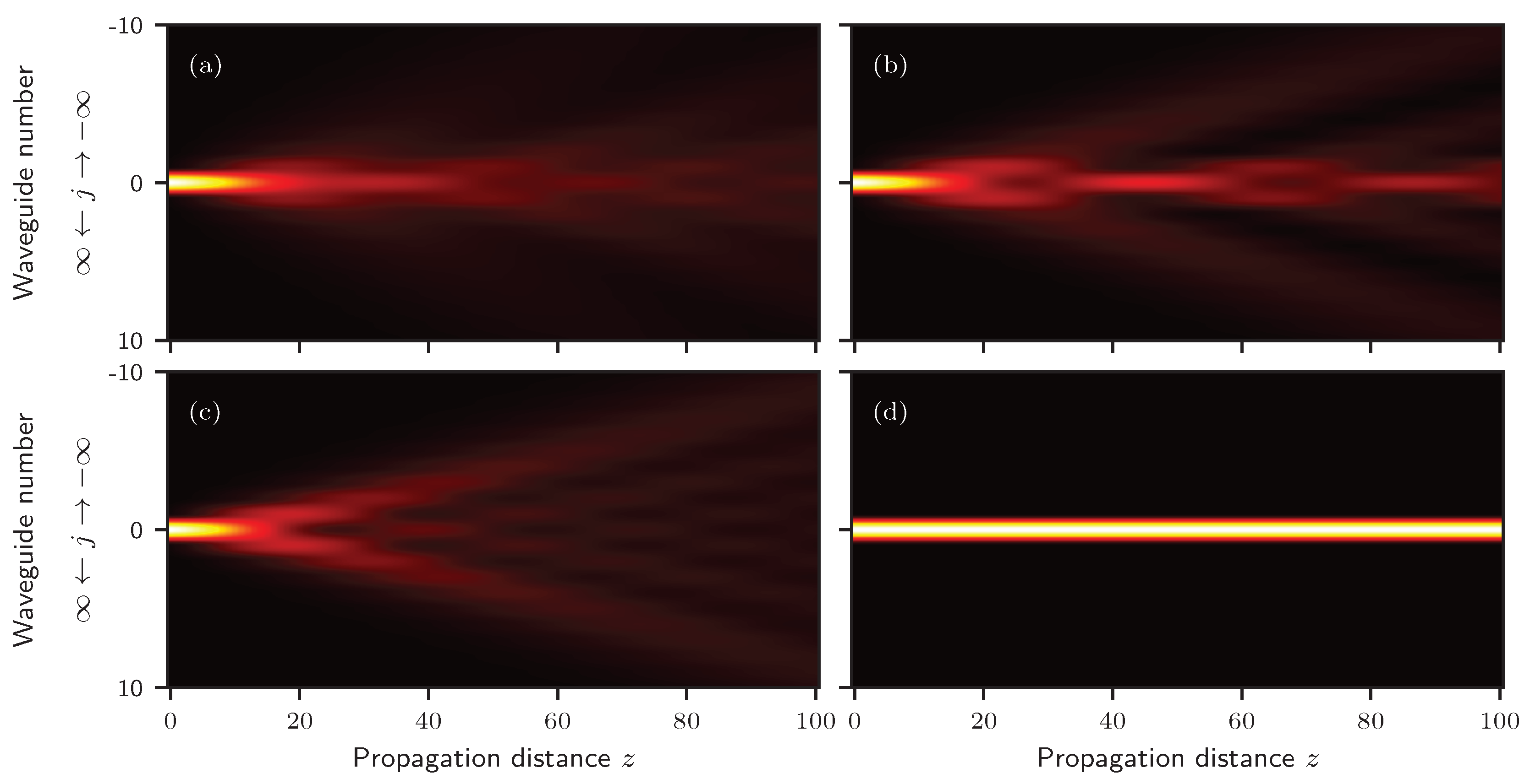
Figure 2 illustrates the light intensity distribution as a function of the propagation distance z for different coupling functions applied in Eq. (24). Panels (a) and (b) correspond to cases where the coupling is defined by natural logarithm and exponential functions, respectively, leading to a slight concentration of light in the central waveguide. Panel (c) exhibits a propagation pattern similar to that observed under nearest-neighbor interactions. Finally, panel (d) describes a nonphysical configuration with zero losses, highlighting the tendency of light to remain localized in the central region.
5. Conclusions
This work investigates the complex dynamics in waveguide arrays by extending the analysis beyond nearest-neighbor interactions to include higher-order couplings. We derive an analytical expression in terms of a generalized Bessel-like function, structurally analogous to the first-neighbor case in an infinite array. Our results show that, for sufficiently strong higher-order coupling, a significant fraction of the propagating light remains localized around the initially excited waveguide. Finally, we discuss the passage from discrete to continuous formulations relating the field amplitudes and the Fourier-series coefficients of a specified function and illustrate these concepts with figures depicting intensity distributions under varied coupling scenarios.
References
- Heitler, W. The Quantum Theory of Radiation; Dover Books on Physics, Dover Publications, 1984. [Google Scholar]
- Gyongyosi, L.; Imre, S. A Survey on quantum computing technology. Computer Science Review 2019, 31, 51–71. [Google Scholar] [CrossRef]
- Fedida, S.; Serafini, A. Tree-level entanglement in quantum electrodynamics. Phys. Rev. D 2023, 107, 116007. [Google Scholar] [CrossRef]
- Vidal, G. Efficient Classical Simulation of Slightly Entangled Quantum Computations. Phys. Rev. Lett. 2003, 91, 147902. [Google Scholar] [CrossRef] [PubMed]
- Feynman, R.P. Simulating physics with computers. In Feynman and computation; CRC Press, 2018; pp. 133–153. [Google Scholar]
- Blatt, R.; Wineland, D. Entangled states of trapped atomic ions. Nature 2008, 453, 1008–1015. [Google Scholar] [CrossRef] [PubMed]
- Monroe, C.; Campbell, W.C.; Duan, L.M.; Gong, Z.X.; Gorshkov, A.V.; Hess, P.W.; Islam, R.; Kim, K.; Linke, N.M.; Pagano, G.; et al. Programmable quantum simulations of spin systems with trapped ions. Rev. Mod. Phys. 2021, 93, 025001. [Google Scholar] [CrossRef]
- Bloch, I.; Dalibard, J.; Zwerger, W. Many-body physics with ultracold gases. Rev. Mod. Phys. 2008, 80, 885–964. [Google Scholar] [CrossRef]
- Mivehvar, F.; Piazza, F.; Donner, T.; and, H.R. Cavity QED with quantum gases: new paradigms in many-body physics. Advances in Physics 2021, 70, 1–153. [Google Scholar] [CrossRef]
- Bohrdt, A.; Homeier, L.; Reinmoser, C.; Demler, E.; Grusdt, F. Exploration of doped quantum magnets with ultracold atoms. Annals of Physics 2021, 435, 168651. [Google Scholar] [CrossRef]
- Christodoulides, D.N.; Lederer, F.; Silberberg, Y. Discretizing light behaviour in linear and nonlinear waveguide lattices. Nature 2003, 424, 817–823. [Google Scholar] [CrossRef]
- Barral, D.; Walschaers, M.; Bencheikh, K.; Parigi, V.; Levenson, J.A.; Treps, N.; Belabas, N. Quantum state engineering in arrays of nonlinear waveguides. Phys. Rev. A 2020, 102, 043706. [Google Scholar] [CrossRef]
- Urzúa, A.R.; Ramos-Prieto, I.; Moya-Cessa, H.M. Integrated optical wave analyzer using the discrete fractional Fourier transform. J. Opt. Soc. Am. B 2024, 41, 2358–2365. [Google Scholar] [CrossRef]
- Rai, A.; Das, S.; Agarwal, G. Quantum entanglement in coupled lossy waveguides. Opt. Express 2010, 18, 6241–6254. [Google Scholar] [CrossRef] [PubMed]
- Perez-Leija, A.; Szameit, A.; Ramos-Prieto, I.; Moya-Cessa, H.; Christodoulides, D.N. Generalized Schrödinger cat states and their classical emulation. Phys. Rev. A 2016, 93, 053815. [Google Scholar] [CrossRef]
- Perets, H.B.; Lahini, Y.; Pozzi, F.; Sorel, M.; Morandotti, R.; Silberberg, Y. Realization of quantum walks with negligible decoherence in waveguide lattices. Phys. Rev. Lett. 2008, 100, 170506. [Google Scholar] [CrossRef]
- Peruzzo, A.; Lobino, M.; Matthews, J.C.; Matsuda, N.; Politi, A.; Poulios, K.; Zhou, X.Q.; Lahini, Y.; Ismail, N.; Wörhoff, K.; et al. Quantum walks of correlated photons. Science 2010, 329, 1500–1503. [Google Scholar] [CrossRef]
- Biggerstaff, D.N.; Heilmann, R.; Zecevik, A.A.; Gräfe, M.; Broome, M.A.; Fedrizzi, A.; Nolte, S.; Szameit, A.; White, A.G.; Kassal, I. Enhancing coherent transport in a photonic network using controllable decoherence. Nat Commun 2016, 7, 11282. [Google Scholar] [CrossRef]
- Lahini, Y.; Avidan, A.; Pozzi, F.; Sorel, M.; Morandotti, R.; Christodoulides, f.D.N.; Silberberg, Y. Anderson localization and nonlinearity in one-dimensional disordered photonic lattices. Phys. Rev. Lett. 2008, 100, 013906. [Google Scholar] [CrossRef]
- Keil, R.; Perez-Leija, A.; Dreisow, F.; Heinrich, M.; Moya-Cessa, H.; Nolte, S.; Christodoulides, D.N.; Szameit, A. Classical Analogue of Displaced Fock States and Quantum Correlations in Glauber-Fock Photonic Lattices. Phys. Rev. Lett. 2011, 107, 103601. [Google Scholar] [CrossRef] [PubMed]
- Keil, R.; Perez-Leija, A.; Aleahmad, P.; Moya-Cessa, H.; Nolte, S.; Christodoulides, D.N.; Szameit, A. Observation of Bloch-like revivals in semi-infinite Glauber-Fock photonic lattices. Opt. Lett. 2012, 37, 3801–3803. [Google Scholar] [CrossRef]
- Efremidis, N.K.; Christodoulides, D.N. Discrete solitons in nonlinear zigzag optical waveguide arrays with tailored diffraction properties. Phys. Rev. E 2002, 65, 056607. [Google Scholar] [CrossRef]
- Szameit, A.; Pertsch, T.; Nolte, S.; Tünnermann, A.; Lederer, F. Long-range interaction in waveguide lattices. Phys. Rev. A 2008, 77, 043804. [Google Scholar] [CrossRef]
- Tapia-Valerdi, M.A.; Ramos-Prieto, I.; Soto-Eguibar, F.; Moya-Cessa, H.M. Waveguide arrays interaction to second neighbors: Exact solution. arXiv preprint 2025. [Google Scholar]
- Stockhofe, J.; Schmelcher, P. Bloch dynamics in lattices with long-range hopping. Phys. Rev. A 2015, 91, 023606. [Google Scholar] [CrossRef]
- Longhi, S.; Marangoni, M.; Lobino, M.; Ramponi, R.; Laporta, P.; Cianci, E.; Foglietti, V. Observation of Dynamic Localization in Periodically Curved Waveguide Arrays. Phys. Rev. Lett. 2006, 96, 243901. [Google Scholar] [CrossRef]
- Anuradha, T.; Patra, A.; Gupta, R.; Rai, A.; Sen(De), A. Production of genuine multimode entanglement in circular waveguides with long-range coupling. Phys. Rev. A 2024, 109, 032411. [Google Scholar] [CrossRef]
- Wang, G.; Huang, J.P.; Yu, K.W. Nontrivial Bloch oscillations in waveguide arrays with second-order coupling. Opt. Lett. 2010, 35, 1908–1910. [Google Scholar] [CrossRef] [PubMed]
- Qi, F.; Feng, Z.; Wang, Y.; Xu, P.; Zhu, S.; Zheng, W. Photon-number correlations in waveguide lattices with second order coupling. J. Opt. 2014, 16, 125007. [Google Scholar] [CrossRef]
- Román-Ancheyta, R.; Ramos-Prieto, I.; Perez-Leija, A.; Busch, K.; León-Montiel, R.d.J. Dynamical Casimir effect in stochastic systems: Photon harvesting through noise. Phys. Rev. A 2017, 96, 032501. [Google Scholar] [CrossRef]
- Villegas-Martínez, B.; Moya-Cessa, H.; Soto-Eguibar, F. Modeling displaced squeezed number states in waveguide arrays. Physica A: Statistical Mechanics and its applications 2022, 608, 128265. [Google Scholar] [CrossRef]
- Dreisow, F.; Wang, G.; Heinrich, M.; Keil, R.; Tünnermann, A.; Nolte, S.; Szameit, A. Observation of anharmonic Bloch oscillations. Opt. Lett. 2011, 36, 3963–3965. [Google Scholar] [CrossRef]
- Ramos-Prieto, I.; Uriostegui, K.; Récamier, J.; Soto-Eguibar, F.; Moya-Cessa, H.M. Kapitza–Dirac photonic lattices. Opt. Lett. 2021, 46, 4690–4693. [Google Scholar] [CrossRef]
- London, F. Über die Jacobischen transformationen der quantenmechanik. Z. Physik 1926, 37, 915–925. [Google Scholar] [CrossRef]
- Susskind, L.; Glogower, J. Quantum mechanical phase and time operator. Physics Physique Fizika 1964, 1, 49–61. [Google Scholar] [CrossRef]
- Carruthers, P.; Nieto, M.M. Phase and Angle Variables in Quantum Mechanics. Rev. Mod. Phys. 1968, 40, 411–440. [Google Scholar] [CrossRef]
- Perez-Leija, A.; Andrade-Morales, L.A.; Soto-Eguibar, F.; Szameit, A.; Moya-Cessa, H.M. The Pegg–Barnett phase operator and the discrete Fourier transform. Physica Scripta 2016, 91, 043008. [Google Scholar] [CrossRef]
- Dattoli, G.; Torre, A.; Lorenzutta, S.; Maino, G.; Chiccoli, C. Theory of generalized Bessel functions.-ii. Il Nuovo Cimento B (1971-1996) 1991, 106, 21–51. [Google Scholar] [CrossRef]
- Dattoli, G.; Chiccoli, C.; Lorenzutta, S.; Maino, G.; Richetta, M.; Torre, A. Generating functions of multivariable generalized Bessel functions and Jacobi-elliptic functions. Journal of Mathematical Physics 1992, 33, 25–36. [Google Scholar] [CrossRef]
- Szameit, A.; Dreisow, F.; Pertsch, T.; Nolte, S.; Tünnermann, A. Control of directional evanescent coupling in fs laser written waveguides. Opt. Express 2007, 15, 1579–1587. [Google Scholar] [CrossRef]
- Szameit, A.; Blömer, D.; Burghoff, J.; Pertsch, T.; Nolte, S.; Tünnermann, A. Hexagonal waveguide arrays written with fs-laser pulses. Appl. Phys. B 2006, 82, 507–512. [Google Scholar] [CrossRef]
- Gradshteyn, I.; Ryzhik, I. Table of Integrals, Series, and Products; Academic Press, 2014. [Google Scholar]
Figure 1.
The evolution of the squared amplitude modulus in each waveguide is shown for an infinite waveguide array governed by Eq. (11), considering interactions up to fourth neighbors. In panels (a) to (d), the central waveguide () is initially excited. The coupling constants decrease progressively, taking the values , , , and .
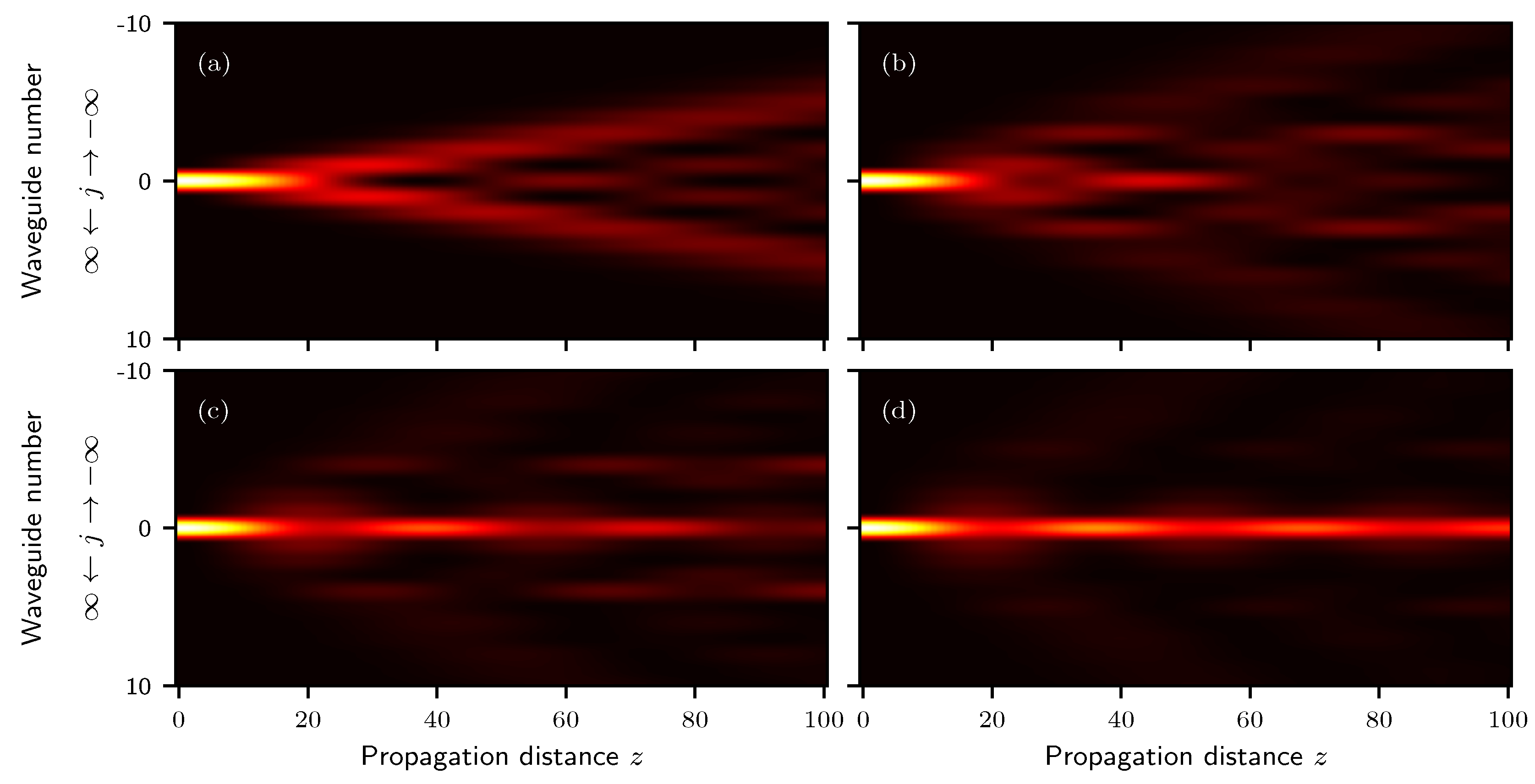
Figure 2.
The intensity evolution of the field in an infinite waveguide array described by Eq. (24), is shown for different functions when the central waveguide is illuminated; (a) corresponds to (25) with , (b) to (26) with the same parameter value, (c) represents (27), and (d) illustrates (26) again with
Disclaimer/Publisher’s Note: The statements, opinions and data contained in all publications are solely those of the individual author(s) and contributor(s) and not of MDPI and/or the editor(s). MDPI and/or the editor(s) disclaim responsibility for any injury to people or property resulting from any ideas, methods, instructions or products referred to in the content. |
© 2025 by the authors. Licensee MDPI, Basel, Switzerland. This article is an open access article distributed under the terms and conditions of the Creative Commons Attribution (CC BY) license (http://creativecommons.org/licenses/by/4.0/).
Copyright: This open access article is published under a Creative Commons CC BY 4.0 license, which permit the free download, distribution, and reuse, provided that the author and preprint are cited in any reuse.


