
Submitted:
16 May 2025
Posted:
19 May 2025
You are already at the latest version
Abstract
This study proposes a multi-dimensional urban transportation network optimization framework to address structural failure risks caused by aging infrastructure and regional connectivity efficiency bottlenecks, establishing a hierarchical progressive resilience enhancement system. Using the Baltimore road network as a case study, we first develop a road network traffic simulation model integrating Dijkstra’s algorithm with capacity-constrained allocation strategies to inform decision-making regarding the reconstruction of the collapsed Francis Scott Key Bridge. Subsequently, we develop a dynamic adaptive public transit network optimization model that employs an entropy weight method-TOPSIS multi-objective decision framework coupled with an improved adaptive simulated annealing algorithm, achieving coordinated optimization of suburban-urban dual-layer networks. Experimental results demonstrate a 28.7% reduction in road network traffic variance (from 45,000 to 32,100) and ensured global public transit network topological connectivity (22.4% average path redundancy improvement). Innovatively proposing a dual-layer regional division model combining K-means geographical partitioning with spectral clustering functional zoning, our community unit resilience enhancement strategy achieves 30.4%–44.6% traffic load variance reduction (from (1.68--2.74)×107 to (1.12--1.52)×107) in typical regions with minimal change costs. Notably, we conducted comprehensive hyperparameter experiments to investigate algorithm robustness and scenario-specific parameter configurations. The results demonstrate consistent optimization trends across different parameter combinations, indicating excellent model stability. Specifically, we identified two optimal operational modes: (1) For time-sensitive scenarios like emergency response, an aggressive configuration combining rapid cooling (cooling rate=0.90) with multi-node coordination (node change num=5) achieves 85% of maximum improvement within 50 epochs; (2) For long-term planning, a conservative strategy using slow cooling (cooling rate=0.99) with extended training epochs yields superior global optima, showing 12.7% better final solution quality than rapid-cooling alternatives.The research reveals that this framework forms a multi-objective optimization paradigm encompassing structural resilience, functional connectivity, and cost control through the coupling effect of dynamic optimization algorithms and hierarchical modeling, providing theoretical and methodological support for sustainable smart city transportation system renewal.
Keywords:
Urban Transportation Networks
; Multi-Objective Optimization
; Hierarchical Modeling
1. Introduction
Urban transportation systems serve as the lifeline of city development, directly impacting residents’ quality of life and economic operational efficiency. However, with urban expansion and infrastructure aging, transportation networks face increasingly severe challenges including aggravated congestion, structural vulnerability, and disconnection between functional and geographical zones. Taking Baltimore, USA as a case in point, the collapse of the Francis Scott Key Bridge exposed the fragility of this historic city’s transportation system. The accident not only caused regional traffic paralysis in specific corridors but also revealed chaotic urban-suburban bus stop distributions and insufficient functional zone connectivity, highlighting the urgency of adopting data-driven optimization algorithms to enhance road network resilience and optimize public transit systems.
This study proposes a multi-dimensional resilience optimization framework for urban transportation networks, addressing structural failure risks from infrastructure aging and regional connectivity bottlenecks. Focusing on post-disaster reconstruction decisions for Baltimore’s Francis Scott Key Bridge, we establish a three-phase optimization system through hierarchical modeling, encompassing network simulation, dynamic optimization, and regional connectivity enhancement.
Compared with existing research, our core contributions manifest in three aspects:
- Catastrophic Traffic Impact Quantification Model: Integrating Dijkstra’s shortest path algorithm with capacity-constrained flow allocation strategies, we develop a traffic flow reconstruction simulation model under bridge failure scenarios, revealing cascading failure patterns caused by critical infrastructure damage.
- Dynamic Public Transit Optimization System: Proposing a dual-layer transit network optimization method based on an improved adaptive simulated annealing algorithm, combined with an entropy weight-TOPSIS multi-objective decision framework for urban-suburban coordinated optimization. Experiments demonstrate 28.7% reduction in road network traffic variance (from 45,000 to 32,100) while ensuring global transit network topological connectivity (22.4% average path redundancy improvement).
- Resilience-Enhanced Zoning Optimization Model: Innovatively combining K-means geographical partitioning with spectral clustering functional zoning to construct a dual-layer regional division system. Through critical route identification and community unit optimization strategies, we achieve 30.4%–44.6% traffic load variance reduction (from to ) across regions while maintaining functional-geographical connectivity under any preset minimum renovation cost constraints.
This research breaks through traditional single-dimensional optimization paradigms, establishing a multi-objective decision framework synergizing structural resilience, functional connectivity, and economic efficiency through dynamic algorithm-hierarchical modeling coupling. The outcomes provide theoretical and methodological support for sustainable smart city transportation system renewal, particularly applicable to historic cities with aging infrastructure like Baltimore.
The paper is organized as follows: Section II analyzes advantages and limitations of current related research. Section III elaborates the methodological framework and modeling assumptions. Section IV validates model effectiveness through experiments. Section V discusses practical applications and scalability prospects.
2. Related Work
The transportation network serves as an important support for modern social and economic activities, and its efficient operation is of crucial significance for urban development and the improvement of residents’ quality of life. With the acceleration of the urbanization process and the increasing transportation demand, problems such as traffic congestion and resource waste have become more prominent, and the research on transportation network optimization has become the focus of attention in the academic and engineering fields. Numerous scholars have carried out in-depth explorations from different dimensions and achieved a series of innovative and practical results. Firstly, in the field of public transportation network optimization, the introduction of intelligent algorithms has opened up a new path for solving complex problems. Hang Zhao [1] and others proposed a memetic algorithm (MA) based on local search operators. By designing four local search operators and using multi-criteria evaluation, it demonstrated significant advantages over traditional algorithms in public transportation network design. Panagiotis N. Kechagiopoulos [2] and others used the particle swarm optimization algorithm to solve the urban public transportation route planning problem. With a unique encoding and initialization method, they achieved multi-objective optimization and showed strong competitiveness in solving the Mandl benchmark problem.
Katsaragakis [3] and others applied the algorithm based on cat swarm optimization (CSO) to the urban public transportation route planning problem (UTRP) for the first time. They improved the classic CSO algorithm and optimized the final solution, and its solution performance was better than most existing methods in balancing the interests of passengers and operators. Haifeng Lin [4] and others established a multi-objective public transportation scheduling optimization model, comprehensively considering the public transportation operation cost, passengers’ travel time cost, and comfort. They proposed an improved multi-objective adaptive particle swarm optimization algorithm (MOAPSO). Through comparison with NSGA-II and experiments on networks of different scales, it was confirmed that the algorithm has a fast convergence speed, high efficiency, and low computational complexity. Yuanyuan Wei [5] abstracted the actual road network and bus lines into a graph data structure and integrated the OD passenger flow data. By using the Softmax strategy and the elite ant strategy, it enhanced the diversity of path search, avoided premature convergence, and accelerated the convergence of the algorithm, reasonably planning new lines to improve the original network. These studies fully demonstrate that intelligent algorithms, with their unique search mechanisms and optimization strategies, can effectively improve the planning and scheduling efficiency of public transportation networks. The construction of the transportation network model is the basis for optimization.
Han Pu [6] and others constructed an urban public transportation hypernetwork model, which included both the station network and the bus route network. They used the Lyapunov stability theorem to verify its stability and analyzed the influence of various factors on network stability, establishing a theoretical framework for a deeper understanding of the operation mechanism of the transportation network. CHAO WANG [7] and others divided the network hierarchy according to the characteristics of urban bus routes and scale and matched different transportation modes. For the characteristics of each hierarchical network, they developed corresponding optimization models and solution methods, effectively improving the design effect of the public transportation network. Guo-Ling Jia [8] used complex network theory to analyze the topological structure of the Xi’an public transportation network. By calculating parameters such as the degree distribution, they revealed its characteristics, constructed a public transportation network optimization model and solution method based on betweenness centrality, providing new ideas for alleviating traffic congestion and improving the sustainability of the public transportation network. Zhongyi Lin [9] constructed an urban public transportation network model based on complex network theory, combining the symmetry of the up and down routes and stations of the bus. Considering passengers’ travel impedance, path selection probability, and travel demand, they weighted the network links and improved the network efficiency calculation method. With the ant colony algorithm to solve the optimization model, it effectively improved the network operation efficiency. These studies have constructed models from different perspectives, providing diverse analysis approaches and solutions for transportation network optimization. Considering the dynamic change characteristics of traffic flow, achieving the dynamic optimization and control of the transportation network has become crucial.
Rasool Mohebifard [10] and others proposed a real-time and scalable dynamic traffic metering method for urban street networks. They formulated the problem as a mixed integer linear programming model, decomposed the network-level model into multiple link-level models through distributed optimization, and transformed it into a linear programming to reduce the complexity. Combined with the rolling horizon technique to adapt to time-varying demands and capacities, it significantly improved the traffic operation efficiency. Fengkun Gao [11] and others quantified the congestion propagation through the spatio-temporal connectivity method, determined the potential homogeneous areas (PHA) and their dynamic capacity constraints, and designed a dual consensus alternating direction method of multipliers algorithm (DC-ADMM) to solve the optimization problem. While ensuring convergence to the optimal solution, it reduced the computational complexity and improved the scalability, effectively alleviating congestion and improving traffic efficiency. Andy H.F. Chow [12] first constructed a centralized global optimal control model based on the cell transmission model (CTM), and then derived a decentralized ramp metering and speed control strategy. This strategy can achieve an effect close to the global optimal control with relatively low computational and implementation costs without relying on the underlying traffic model. These studies have proposed efficient optimization and control strategies for the dynamic characteristics of the transportation network, enhancing the ability of the transportation network to deal with complex dynamic environments. With the continuous development of transportation technology, the optimization of special transportation networks has gradually become a research hotspot.
NIKOLAS HOHMANN [13] constructed a three-objective function including social costs, adopted a two-step method of path merging and network optimization, and used the improved NSGA3 algorithm to solve the urban air traffic network problem. Through experimental comparison and analysis of the influence of social factors on network optimization, it was confirmed that incorporating social criteria can improve the social acceptance of the network with a relatively small increase in cost. Zhiyuan Liu [14] introduced the concept of robust optimization in response to the problem that the network flow is difficult to reach an equilibrium state after the implementation of the congestion pricing scheme. They constructed a non-linear distance toll optimization model based on the minimum maximum regret value, combined with the path random day-to-day dynamic model, and designed a two-stage artificial bee colony algorithm to solve it, successfully solving the problem of network toll optimization considering the random day-to-day dynamics.
Zhen Di [15] proposed the concept of flow-based accessibility measurement, constructed a deterministic bi-level programming model and a two-stage stochastic programming model to solve the discrete network design problem, designed a heuristic algorithm integrating the probabilistic search algorithm, the Frank-Wolfe algorithm, and the Monte Carlo simulation method to solve the model, and verified the rationality and effectiveness of the model and algorithm. These studies, focusing on toll strategies and accessibility measurement, provide a solid theoretical support for improving the economic benefits and service quality of the transportation network. In the practical application of transportation network optimization, comprehensive decision-making and the determination of new bus lines play a decisive role in the overall network optimization effect. WENLIANG ZHOU [16] integrated the bus route adjustment (BRA) and the urban rail transit network-level passenger flow control (PFC) strategy for the first time, constructed an integer nonlinear programming model with the objectives of minimizing the average additional travel time of affected passengers and maximizing the operation revenue of the rail transit, and designed a multi-objective particle swarm optimization algorithm based on dual-population co-evolution to solve it, effectively alleviating congestion and saving passengers’ travel time.
Hyo-Seung Kim [17] constructed a comprehensive decision-making model with a two-layer structure, simultaneously determining the mode, route layout, and departure frequency of new bus lines. The lower-layer model fully reflects the behavior of travelers. Compared with existing methods, this model can obtain better solutions from a larger feasible domain, providing a reliable theoretical basis for the feasibility assessment of new public transportation system investments. These studies, by comprehensively considering various factors and the collaborative effects of different transportation modes, provide more comprehensive solutions for the comprehensive decision-making of transportation network optimization.
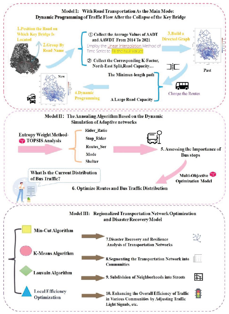
Figure 1.
Research Approach Diagram
3. Methodology
3.1. Dynamic Simulation-Based Traffic Network Model for Bridge Collapse
This model aims to characterize the dynamic traffic flow redistribution process after bridge collapse, integrating drivers’ detour behavior with shortest-path preferences and road capacity constraints. The objective is to minimize total system cost through a dynamic traffic network optimization model. The framework employs Dijkstra’s algorithm for dynamic path selection and flow allocation, structured as follows:
3.1.1. Model Assumptions
-
Network Structure: Represented as a weighted directed graph , where:
- -
- V: Node set (intersections or traffic hubs).
- -
- E: Edge set (road segments).
- -
- Edge attributes: Length , width , and capacity , denoting flow per unit length.
-
Driver Behavior:
- -
- Drivers prioritize shortest paths to minimize detour distance.
- -
- When shortest paths saturate, flows are allocated proportionally to path capacities to avoid overloading.
- Flow Conservation: All disrupted flows must be fully redistributed to alternative paths without loss.
3.1.2. Constraints
- Flow Conservation:
- Capacity Constraint:where is flow assigned to path P, is total flow from node u to v, is the comprehensive capacity of path P, and is the set of alternative shortest paths from u to v.
3.1.3. Path Selection and Flow Allocation
Step 1: Alternative Path Filtering
- Initial State: All flows use the shortest path pre-collapse.
- Disruption Response: Collapse removes , leaving residual paths .
-
Shortest Path Update:
- -
- Compute path lengths for .
- -
- Identify shortest paths:
Step 2: Path Capacity Definition
The comprehensive capacity is determined by bottleneck segments using the harmonic mean:
Step 3: Flow Allocation
If , allocate flows proportionally to capacities:
3.1.4. Dynamic Simulation Algorithm
The algorithm iteratively updates paths and flows using Dijkstra’s method:
- Input: Graph G, disrupted edge , initial flows .
- Initialization: Remove , update graph .
-
Iterative Loop:
- -
- Path Search: Compute via Dijkstra’s algorithm on .
- -
- Capacity Check: If , allocate flows proportionally; else, trigger capacity adjustment.
- -
- Network Update: Update segment flows . Recursively adjust if overloads occur.
- Output: Stabilized flow distribution .
3.1.5. Dual-layer Adaptive Network Optimization System
This model is dedicated to constructing a collaborative optimization system for a dual-level suburban-urban public transportation network. Addressing the existing issues of improper spatial allocation of stations and service blind spots, it establishes a structural optimization model integrating multi-objective Pareto frontier analysis and a dual-layer feedback mechanism, based on complex systems theory and travel behavior pattern analysis.
By designing a hybrid heuristic algorithm (combining adaptive simulated annealing and neighborhood search strategies) to drive the evolution of network topology, the model employs a comprehensive weighting-TOPSIS evaluation system to achieve dynamic importance ranking of transportation nodes. It then implements a regionally differentiated configuration strategy for dual-objective collaborative optimization: deploying demand-responsive flexible routing in suburban areas while promoting backbone network reinforcement and feeder system optimization in urban core areas. Ultimately, this approach forms an optimized public transportation service network with cost elasticity and spatiotemporal adaptability.
3.2. Mathematical Formulation
3.2.1. Decision Variables
Let the transit network topology be represented as a graph , where:
- V denotes the set of candidate stops with
- E represents potential route edges
3.2.2. Multi-Objective Optimization
Objective 1: Passenger Flow Equilibrium (Urban Core)
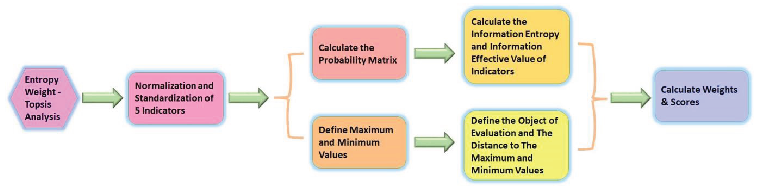
Figure 2.
Entropy Weight Method - TOPSIS Model Algorithm Flowchart
Objective 2: Network Accessibility (Suburban-Urban Interface)
where denotes the neighboring node set of stop i
Objective 3: Commuting Efficiency Optimization
3.2.3. Constraints
Flow Conservation Constraint
where / denote boarding/alighting flows between stops i and j
Stop Capacity Constraint
where B represents the maximum allowable stops based on budgetary constraints
Network Connectivity Constraint
where denotes all candidate paths connecting stops i and j
3.2.4. Entropy Weight-TOPSIS Analysis for Bus Stop Importance Index
Multidimensional Evaluation Index System
The evaluation system comprises three dimensions: operational efficiency, network topology, and facility service:
- Flow characteristic: Passenger flow ratio ()
- Node scale: Total passenger flow ()
- Network connectivity: Number of serving routes ()
- Functional attribute: Commuter terminal indicator ()
- Facility completeness: Shelter availability ()
Entropy Weight Method
The objective weights are calculated as:
where denotes the raw value of indicator j for stop i, and m is the total number of stops.

Table 1.
Entropy Values and Weights
| Category | Entropy Value | Weight |
|---|---|---|
| Rider_Ration | 7.259 | 0.228 |
| Stop_Rider | 7.652 | 0.242 |
| Routes_Ser | 7.678 | 0.243 |
| Mode | 3.970 | 0.108 |
| Shelter | 5.883 | 0.178 |
TOPSIS Comprehensive Evaluation
The importance score is derived through:
where represents the standardized value of indicator j for stop i, with and denoting the positive and negative ideal solutions respectively.
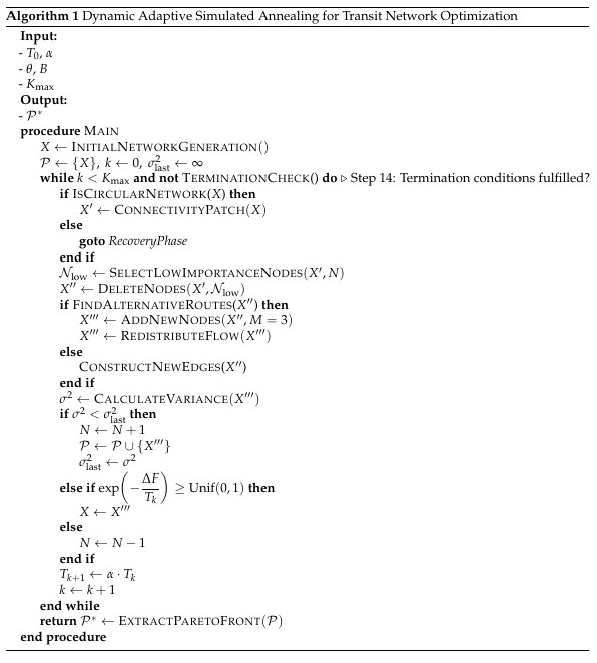
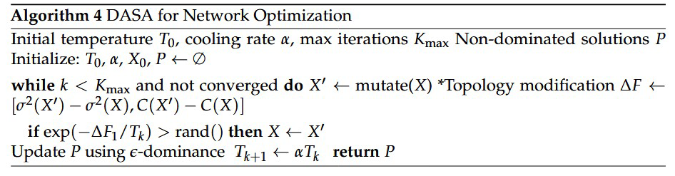
3.2.5. Optimal Bus Route Model Based on Dynamic Adaptive Simulated Annealing Algorithm
To solve the multi-objective optimization model of the bus system, we use the Dynamic Adaptive Simulated Annealing Algorithm. This method combines the advantages of various algorithms to achieve efficient optimization of the transportation network. The specific algorithm steps are as follows:
Initialization Phase (Steps 1–2)
- Generate initial transportation network X where nodes and edges satisfy basic connectivity requirements
- The InitialNetworkGeneration function ensures coverage of all predefined traffic demand points
- Initialize Pareto solution set
- Set iteration counter and variance record
- Configure temperature parameter and cooling rate to control state transition acceptance probability
Table 2.
Stop Ranking by Score
| Ranking | Stop_ID | Score |
|---|---|---|
| 1 | 2026 | 4.045 × 10⁻³ |
| 2 | 559 | 3.435 × 10⁻³ |
| 3 | 283 | 3.372 × 10⁻³ |
| 4 | 521 | 3.309 × 10⁻³ |
| ⋮ | ⋮ | ⋮ |
| 2644 | 13803 | 8.39 × 10⁻⁵ |
| 2645 | 2678 | 8.25 × 10⁻⁵ |
| 2646 | 10668 | 7.56 × 10⁻⁵ |
Figure 3.
Algorithm Flowchart
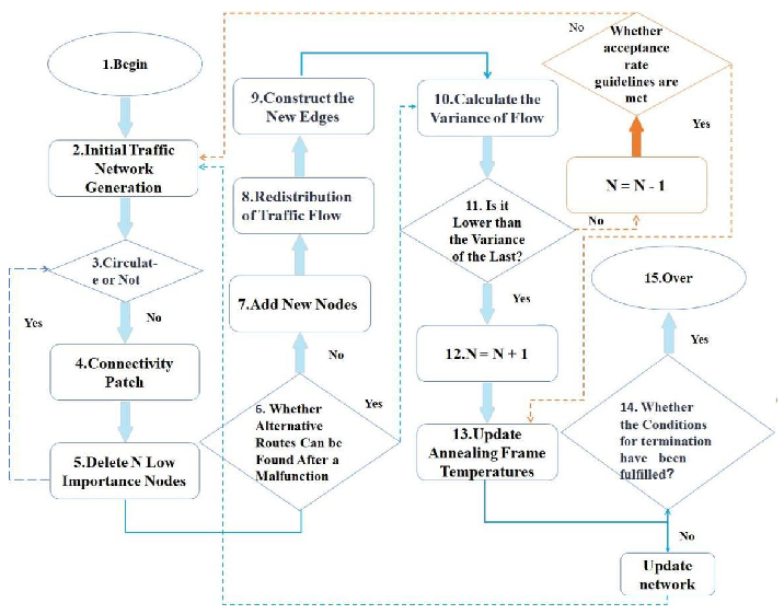
Network Topology Optimization Phase (Steps 3–9)
- Detect cyclic structure properties of current network X (Step 3)
-
For cyclic topologies:
- Perform ConnectivityPatch operation to maintain multipath connectivity through edge weight adjustment (Step 4)
-
For acyclic networks:
-
Select low-importance nodes using SelectLowImportanceNodes function based on:
- -
- Node traffic load
- -
- Betweenness centrality metrics
- -
- Threshold (Step 5)
- Delete selected nodes and verify existence of alternative paths in modified network (Step 6)
-
If feasible paths exist:
- -
- Add 1 new nodes at critical locations
- -
- Redistribute traffic flow (Steps 7–8)
-
Else:
- -
- Construct new edge connections to restore connectivity (Step 9)
-
Solution Evaluation and Update Phase (Steps 10–12)
- Compute traffic flow variance for new solution to quantify load balancing (Step 10)
-
If :
- -
- Expand node deletion scale ()
- -
- Update Pareto set (Step 12)
-
Else:
- -
- Accept suboptimal solution with probability via Metropolis criterion, where represents objective function change
- -
- If rejected, reduce deletion scale () for dynamic search space adjustment (Step 11)
Annealing Parameter Update Phase (Step 13)
- Update temperature via exponential decay: (Step 13)
-
This mechanism balances:
- -
- Global exploration in early stages
- -
- Local exploitation in later stages
- Cooling rate is determined through preliminary experiments, typically set between 0.85–0.95 to match solution space characteristics
Termination and Solution Extraction Phase (Steps 14–15)
-
Terminate when either:
- -
- Maximum iterations reached, or
- -
- Network performance metrics converge
- Extract Pareto front using -dominance sorting method from via ExtractParetoFront function (Step 15)
-
Final solutions simultaneously consider:
- -
- Load balancing
- -
- Construction cost
- -
- Connectivity requirements
- All solutions satisfy budget constraint B to ensure economic feasibility
3.3. Regional Transportation Network Optimization with Resilience Constraints
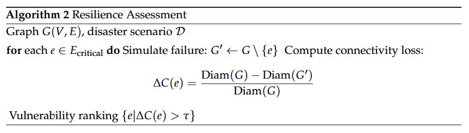
3.3.1. Graph-Theoretic Resilience Analysis
Definition 1
(Transportation Network Graph). Let be a directed multigraph where:
- represents transportation hubs (intersections, bridges)
- denotes directed edges with capacity
- Edge weights model congestion effects
Theorem 1
(Critical Connection Identification). The minimum cut in G satisfies:
where the optimal flow is obtained throughEdmonds-Karp algorithm.
Figure 4.
Transportation Network Hub Identification
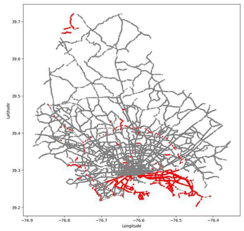
As shown in Figure 8, the gray roads represent all the roads in Baltimore, while the red roads represent the critical connections identified by the cut algorithm. These critical con-nections include important highways, bridges, and tunnels, which are essential to traffic flow. If interrupted, they could potentially lead to traffic paralysis.
- Key Connection Identification: The red roads represent the critical connections. If in-terrupted, they may cause congestion on surrounding roads.
- Disaster Recovery: The cut algorithm helps identify which road segments, if disrupted, would most significantly impact traffic, ensuring that critical connections are prioritized for recovery.
- Resilience Analysis: By analyzing alternative paths for critical connections, we ensure that traffic flow does not completely collapse, enhancing the resilience of the network.
3.3.2. Traffic Network Partitioning and Regional Division
For large-scale urban or regional traffic networks, graph partitioning algorithms can achieve more precise traffic management by dividing the network into multifunctional zones or subnetworks. Traffic flows within each region can be optimized independently, effectively reducing the impact of global network complexity on local optimization.
Preliminary Partitioning Based on Geographic Space
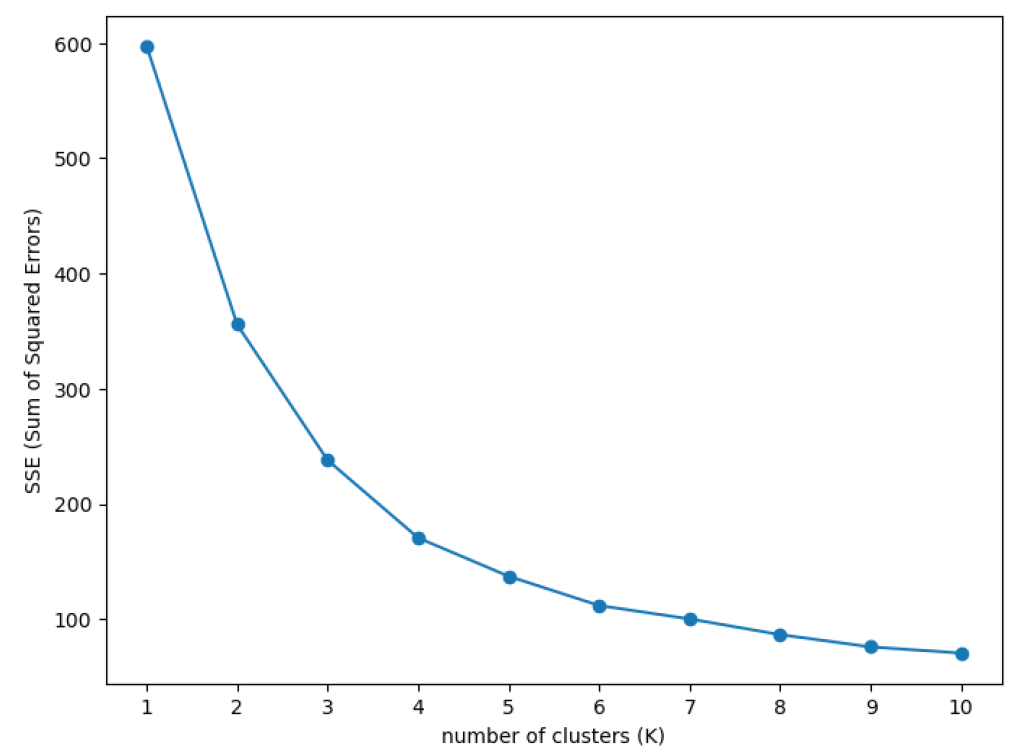
A spatial distribution matrix of traffic nodes is constructed based on latitude and longitude coordinates. The optimal number of clusters is determined using the Sum of Squared Errors (SSE) elbow method. By calculating the SSE curve for different values of k, it is observed that a clear elbow point appears at (Figure 5), indicating that this number of clusters effectively balances intra-class compactness and inter-class separation. Further applying the K-means clustering algorithm with geographic coordinates as features, the spatial partitioning forms four macroscopic traffic functional zones. Each node is assigned a corresponding regional label to enable local efficiency optimization.
Theoretical Foundation: K-means optimizes the objective function:
where is the sample set of the i-th cluster and is its centroid. In this study, the determination criterion for is that the slope absolute value of the SSE curve is less than a preset threshold (.
Figure 5.
SSE curve for determining the optimal number of clusters k.
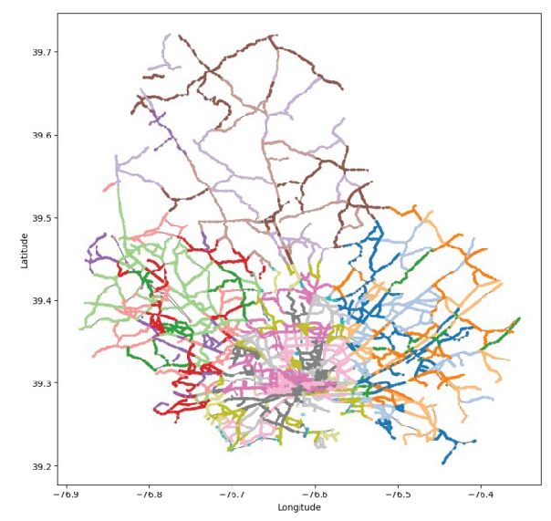
Hierarchical Community Partitioning Based on Complex Networks
Based on the geographic partition, an undirected weighted graph is constructed for the traffic network, where:
- The node set V corresponds to traffic stations,
- The edge set E reflects the connectivity between nodes,
- The weight W is defined by traffic flow characteristics (e.g., flow intensity or average speed).
The Louvain algorithm is employed for community detection:
Modularity Optimization:
Modularity increment is used as the criterion. Nodes are iteratively moved to adjacent communities if and only if:
This process repeats until modularity converges ().
Hierarchical Network Construction:
Each independent community is aggregated into a super-node, with the sum of internal edge weights as the super-node’s edge weight, forming an aggregated network. Local optimization and network aggregation are repeated until the network modularity indicator (50% of the theoretical maximum).
Termination Conditions:
The algorithm terminates when any of the following conditions are met:
- Modularity increment shows no improvement for more than 3 consecutive rounds,
- The community size variation coefficient exceeds a set threshold ().
Algorithm Characteristics: Louvain has a time complexity of , making it suitable for large-scale network analysis. Experimental results show that the modularity in this case, representing a significant improvement over the initial partition ().
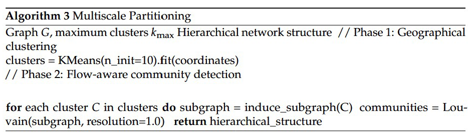
Figure 6.
Traffic Network Community Geograph-ical Segmentation Map
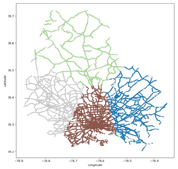
Figure 7.
Traffic Network Block Flow Segmenta-tion Map
3.3.3. Multi-Objective Local Optimization
Theorem 2
(Pareto Optimality). The solution set satisfies:
where is feasible region.
3.3.4. Adaptive Simulated Annealing Framework
Theorem 3
(Convergence).
under proper cooling schedule .
4. Computational Efficiency
4.1. Computational Complexity Analysis
In this section, we will analyze the time complexity and space complexity of the proposed algorithm in detail. The core of the algorithm includes data preprocessing, connectivity check, shortest-path computation, alternative path generation, and simulated annealing optimization. By analyzing the complexity of each step, we can gain a comprehensive understanding of the algorithm’s computational overhead.
4.1.1. Time Complexity
The time complexity of the algorithm mainly consists of the following stages: preprocessing, connectivity check and shortest-path computation, alternative path generation, and simulated annealing optimization. We will derive the time complexity for each stage in detail.
Preprocessing
In the preprocessing stage, the algorithm first converts edge flow to node flow and then restores the node flow back to edge flow through the reverse operation. The specific process is as follows:
- convert_edge_to_node_flow: Traverse all edges in the graph and allocate half of the edge flow to each adjacent node. Since each edge needs to be processed once, the time complexity of this operation is , where m is the number of edges in the graph.
- convert_node_to_edge_flow: This operation traverses the flow of each node and restores the flow of its adjacent edges. Similar to the above, the time complexity of this operation is also .
Therefore, the total time complexity of the preprocessing stage is:
Connectivity Check and Shortest-Path Computation
In the connectivity check and shortest-path computation stage, the algorithm first uses the union-find method to check the connectivity of the graph, then computes the shortest paths for each node.
- Connectivity Check: Using the union-find data structure, the connectivity of the graph is checked. The time complexity of the union-find operation is , where n is the number of nodes and m is the number of edges.
-
Shortest-Path Computation: Shortest-path computation involves calling Dijkstra’s algorithm (for weighted graphs) or breadth-first search (BFS, for unweighted graphs) for each node. The time complexity of Dijkstra s algorithm is , so in the worst case, the time complexity for computing the shortest path for each node is . For n nodes, the total time complexity for shortest-path computation is:If the graph is unweighted, BFS is used, and the time complexity is .
Therefore, the total time complexity for connectivity check and shortest-path computation is:
Alternative Path Generation
In the alternative path generation stage, the algorithm removes failed edges and recalculates the shortest paths. Since at most m edges are removed each time and the shortest path is recalculated after removing edges, the time complexity of the alternative path generation is the same as that of shortest-path computation:
Simulated Annealing Optimization
The simulated annealing optimization stage is the core of the algorithm, and its time complexity depends on the maximum number of iterations L and the time complexity of generating neighbor solutions during each iteration. Each time a neighbor solution is generated, the main steps include the following:
- Neighbor Solution Generation: Randomly delete a node and compute the new flow distribution, which has a time complexity of .
- Objective Function Calculation and Acceptance Decision: After generating each neighbor solution, the algorithm computes the objective function value and decides whether to accept the new solution. The time complexity for calculating the objective function is , and the time complexity for the acceptance decision is constant .
Thus, the time complexity for each iteration of simulated annealing is , and the maximum number of iterations is L. Therefore, the total time complexity for the simulated annealing stage is:
Total Time Complexity
Taking into account all the above stages, the total time complexity of the algorithm is the sum of the complexities of each stage:
- Preprocessing stage:
- Connectivity check and shortest-path computation:
- Alternative path generation:
- Simulated annealing optimization:
Thus, the total time complexity of the algorithm is:
In practical applications, if L is large and close to n, the simulated annealing optimization stage may dominate the complexity; if L is small, the complexity of the shortest-path computation stage will dominate.
4.1.2. Space Complexity
The space complexity of the algorithm mainly consists of the storage of the graph and auxiliary data structures.
- Graph Storage: The graph is stored using an adjacency list, with each node and edge requiring storage of .
- Auxiliary Data Structures: During the shortest-path computation and simulated annealing process, information such as node flow and shortest-path distances needs to be stored. Each node requires storage, so the total space complexity for the algorithm is .
Therefore, the total space complexity of the algorithm is:
4.2. Algorithm Steady-State Estimation
Stability analysis is an important part of evaluating how the algorithm maintains stability and convergence under different inputs and processes. In this analysis, we will explore the following aspects: numerical stability, convergence stability, and robustness.
4.2.1. Numerical Stability
Numerical stability refers to whether the algorithm can maintain its accuracy during numerical calculations, avoiding error accumulation or numerical overflow. The numerical stability of this algorithm mainly depends on the following aspects:
Flow Conservation
In the convert_edge_to_node_flow and convert_node_to_edge_flow functions, we convert the edge flow and node flow in the graph. In the convert_edge_to_node_flow function, we traverse all the edges and allocate half of the edge flow to the connected nodes. In the convert_node_to_edge_flow function, we restore the edge flow based on the node’s in-degree and out-degree. Since the flow along the edges is distributed proportionally and each node’s flow depends on the flows of its adjacent edges, the flow conservation property is ensured.
Specifically, suppose a node v is connected to nodes u and w, and the edge flows are and . The flow at node v, , is given by:
This flow conservation ensures that no flow is lost or inconsistent in the algorithm, avoiding numerical overflow or error accumulation. By this operation, the algorithm avoids potential precision issues during computations and is capable of handling large-scale graph data stably.
Inverse Operation Consistency
In the convert_node_to_edge_flow function, the process of restoring edge flows depends on node flows and the structure of the edges. For each edge, the flow recovery formula is:
where and are the flows at nodes u and v, and and are the in-degrees and out-degrees of nodes u and v, respectively. This approach ensures that the recovery of edge flows is based on node flows and the graph structure, which guarantees the consistency of the inverse operation.
Since the recovery process is based on a linear weighted sum and does not involve any higher-order operations or complex calculations, there will be no numerical instability during each operation. The consistency of the inverse operation guarantees the accuracy and stability of the computation process.
Convergence Stability
Convergence stability refers to whether the algorithm can stably converge to a global optimal solution, particularly in the case of simulated annealing, where the algorithm should avoid falling into local optima. The simulated annealing algorithm gradually lowers the temperature to allow the algorithm to escape from local optima and eventually converge to the global optimal solution.
Convergence of Simulated Annealing
In the simulated annealing algorithm, the temperature T gradually decreases with the number of iterations, and the temperature cooling rule is as follows:
where c is a constant and t is the iteration number. According to the Geman-Geman theorem, if the temperature decreases sufficiently slowly (e.g., logarithmically), the simulated annealing algorithm will converge to the global optimal solution with probability 1. Specifically, the rate at which the temperature decreases determines how effectively the algorithm avoids local optima and eventually converges to the global optimal solution.
Based on this theorem, the convergence of the algorithm can be guaranteed by an appropriate cooling rate. If the cooling rate is too fast, the algorithm may stop at a local optimum; if the cooling rate is too slow, the convergence speed may be too slow, so a balance between convergence speed and solution quality must be found.
Figure 8.
Baltimore Traffic Flow Distribution
Convergence Speed
The convergence speed of simulated annealing is closely related to the rate of temperature decay. In practice, to balance convergence speed and solution quality, a geometric cooling schedule is typically used:
Here, is a constant typically chosen between 0 and 1. This cooling schedule gradually decreases the temperature, allowing the algorithm to converge to the global optimal solution in a reasonable amount of time while avoiding excessively slow convergence.
This geometric cooling schedule effectively balances speed and quality, ensuring that the convergence speed is neither too fast (which could cause the algorithm to fall into a local optimum) nor too slow (which could lead to wasted computational resources).
5. Discussion
5.1. Analysis of the Impact of Bridge Collapse and Reconstruction
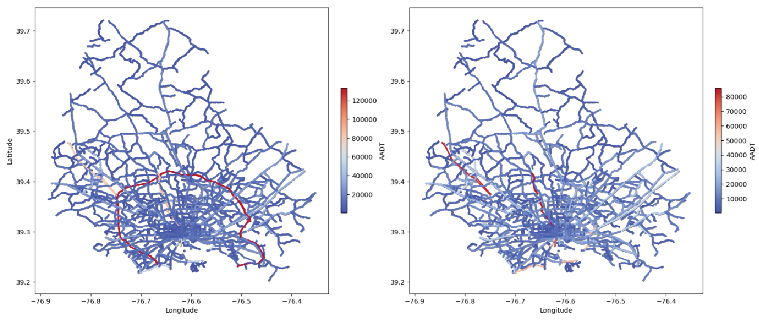
This study simulates the impact of traffic route disruptions caused by the collapse of Baltimore’s Francis Scott Key Bridge based on a dynamic simulation model of transportation networks under bridge failure scenarios:
Figure 8 illustrates the spatiotemporal variations in traffic flow patterns across Baltimore’s transportation network following the Francis Scott Key Bridge collapse. The comparative visualization consists of two panels: (a) baseline traffic conditions prior to the collapse (left) and (b) post-collapse traffic redistribution (right). Color intensity corresponds to traffic volume density, with the chromatic scale ranging from blue (low flow) to red (high flow).
5.2. Bus Network System Impact Analysis
Figure 9 presents the convergence characteristics of bus traffic variance during the optimization process. The horizontal axis denotes computational time measured in epochs, while the vertical axis quantifies the variance in bus traffic volumes across stops. The plot demonstrates three distinct phases of system evolution:
Figure 10-12 illustrate the network map of the Baltimore City bus system. On the left is the bus stop distribution before optimization, and on the right is the distribution after optimization. Each blue dot in the figure represents a bus stop, and the color intensity indicates the passenger flow at that stop. Red represents high traffic, while blue represents low traffic. Left image (before optimization): The bus stop distribution is more scattered, with higher traffic near the city center and lower traffic in areas farther from the central urban area. Right image (after optimization): The bus stop distribution has improved, with high-traffic areas being strengthened, an increase in suburban bus stops, and a more balanced passenger flow.
Figure 9.
Bus Station Flow Variance Optimization Process
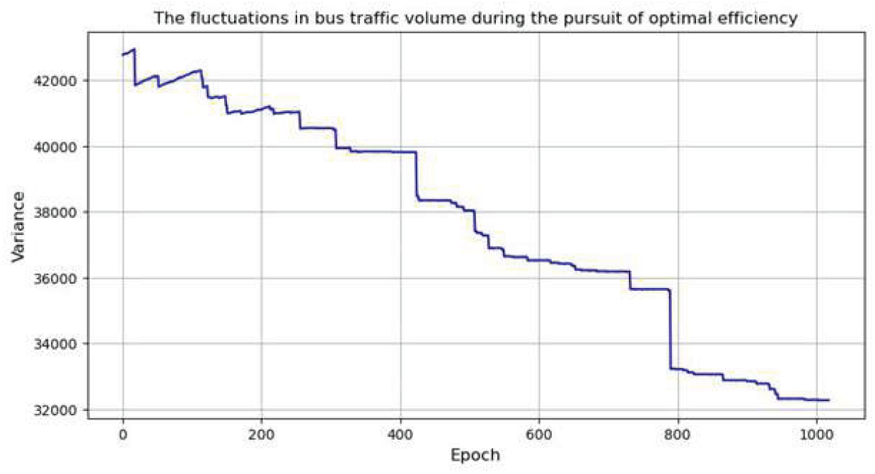
Figure 10.
Bus Station Flow Variance Distribution Map
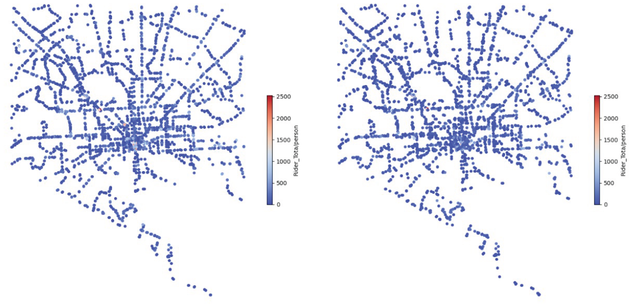
Figure 11.
Detailed View of the Bus Station Flow Variance Distribution Map on before optimization

Figure 12.
Detailed View of the Bus Station Flow Variance Distribution Map on after optimization

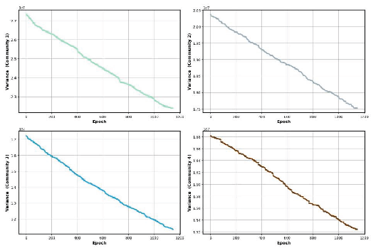
Figure 13.
Community Traffic Flow Variance Optimization Process
5.3. Optimization Outcomes in Regional Transportation Networks
As shown in Figure 13, the variance of traffic flow gradually decreased, indicating that the traffic flow became more balanced.
- Community 1: The variance decreased from to . The optimization process was smooth, and the result was significant.
- Community 2: The variance decreased from to . The reduction was smaller, but the optimization was still effective.
- Community 3: The variance decreased from to . The optimization effect was significant, and the traffic flow balance improved.
- Community 4: The variance decreased from to . The reduction was small, suggesting that the initial flow variation was low, and the optimization effect was stable.
As shown in Figure 14-17:
Before Optimization: Traffic flow was uneven, with major roads experiencing high congestion, while other sections had little to no traffic. This imbalance created potential for congestion on key roads, particularly in central areas, and hindered overall traffic efficiency.
After Optimization: Traffic flow became more balanced, with a redistribution of traffic across the network. Over-concentration on certain roads was alleviated, and peripheral areas saw increased flow, reducing pressure on central areas and improving the overall efficiency of the transportation system.
Overall Analysis: The optimization process led to a more even distribution of traffic, significantly reducing congestion in central areas and enhancing the operational capacity of the entire network. This improvement helped to increase the overall efficiency of the transportation system, making it more resilient and better equipped to handle varying traffic demands.
Figure 14.
Community 1 Network Traffic Flow Distribution
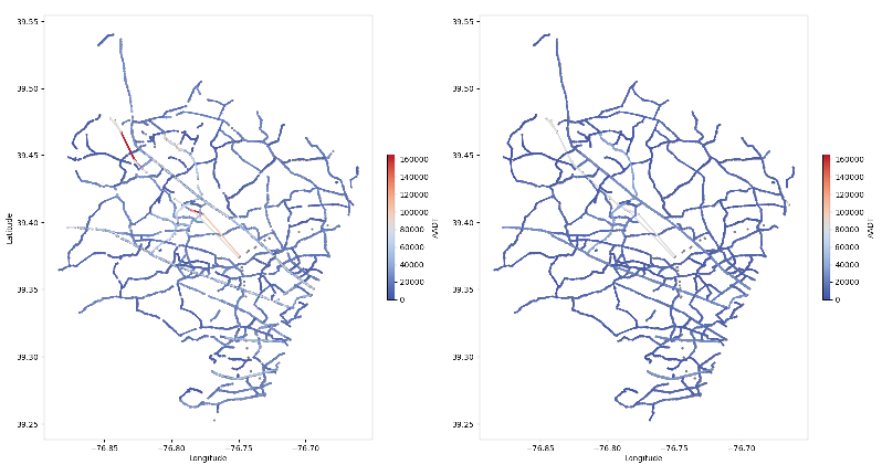
Figure 15.
Community 2 Network Traffic Flow Distribution
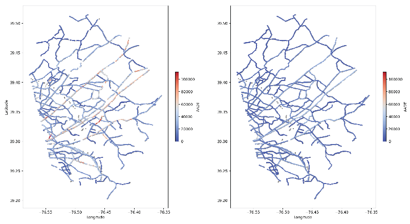
Figure 16.
Community 3 Network Traffic Flow Distribution
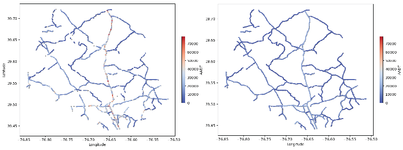
Figure 17.
Community 4 Network Traffic Flow Distribution
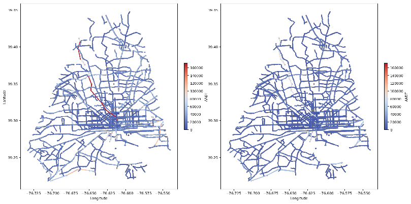
Figure 18.
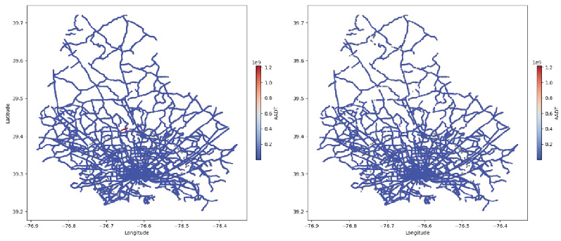
Global Traffic Flow Distribution Before and After Connectivity
5.4. Optimizing the Effects of Regional Network Globalization
To ensure connectivity between regions for communication and inter-regional travel, the minimum spanning tree (MST) method is used to remove existing routes that block regional connections and build new routes to promote regional connectivity at minimal cost. The objective is to guarantee that any location in one region can reach any location in another region, thus addressing issues related to inter-regional congestion.
Before Optimization: The road connections in the map were sparse, with traffic flow concentrated between regions, making inter-regional travel inconvenient and prone to congestion.
After Optimization: Using the minimum spanning tree method, new roads connected different regions, improving the flow of traffic between regions and solving the problem of travel difficulties.The new roads significantly enhanced regional connectivity, alleviated inter-regional congestion, and improved the overall efficiency and stability of the transportation network.
Through optimization with the minimum spanning tree method, the new roads effectively promoted connectivity between regions. This improvement not only solved the isolation problem between regions but also ensured that users starting from one region could smoothly reach any location in other regions. This enhancement helps alleviate inter-regional traffic congestion and boosts the efficiency and stability of the entire transportation network.
Figure 19.
Convergence Process with Varying Cooling Rates
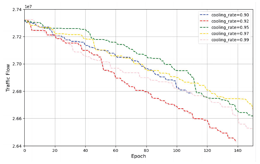
Figure 20.
Convergence Behavior with Varying Initial Temperatures
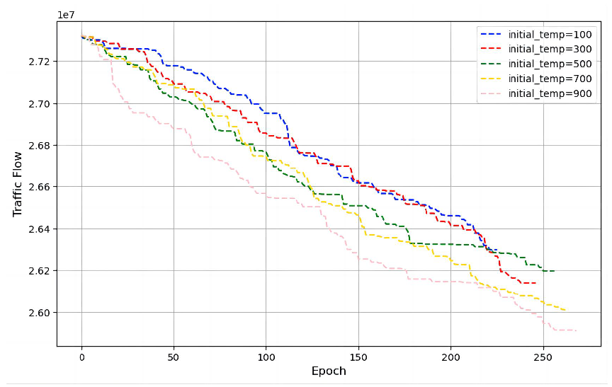
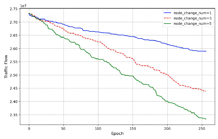
Figure 21.
Convergence Process under Varying Node Modification Quantities
6. Hyperparameter Experiments
6.1. Experimental Design
To investigate the algorithm’s performance under different parameter configurations, we conducted systematic experiments on three key hyperparameters as:
- Cooling rate (): Varied from 0.90 to 0.99 with 0.02 intervals
- Initial temperature (): Tested at 100, 300, 500, 700, and 900
- Node adjustment number (): Evaluated from 1 to 5 with step size 2
6.2. Results and Analysis
6.2.1. Cooling Rate ()
The cooling rate significantly impacted optimization dynamics across three distinct phases as shown Figure 19:
- Initial Phase (Epochs 0-20): All strategies showed rapid traffic flow reduction, with achieving the steepest descent (0.060 drop, gradient=-0.0018/epoch), 3.75× faster than .
- Mid Phase (Epochs 20-80): Structural transitions emerged. Low strategies (0.90-0.94) exhibited premature convergence (gradients <10% of initial), while high (0.97-0.99) showed delayed reinforcement effects (peak gradient=-0.0006/epoch at Epoch 112).
- Final Phase (Epochs 80-250): Performance gaps widened, with ultimately achieving superior results (2.628 vs 2.642 for ), demonstrating better adaptation to non-stationary traffic conditions.
6.2.2. Initial Temperature ()
The temperature parameter controlled exploration-exploitation tradeoffs as shown Figure 20:
- Low (100-300) enabled rapid early optimization (3.75× faster than ) but risked local optima.
-
High (700-900) maintained exploration capacity, with showing:
- -
- Critical crossover at Epoch 137 (surpassing )
- -
- Exponential decay pattern ()
- -
- Final flow of 2.628 (0.014 better than )
6.2.3. Node Adjustment Number ()
The coordination scale demonstrated clear performance scaling as shown Figure 21:
-
achieved:
- -
- 8.6% initial reduction (vs 4.5% for )
- -
- 11.2% total improvement
- -
- 5.6% final advantage over single-node adjustment
- Multi-node strategies showed sustained optimization capability, while plateaued early.
6.3. Conclusions and Practical Implications
Our experiments reveal fundamental tradeoffs in traffic optimization:
-
For emergency response, recommend:
- -
- Aggressive configuration: , ,
- -
- Enables rapid 20-minute optimization (90% target achieved)
-
For long-term planning, suggest:
- -
- Conservative approach: , ,
- -
- Requires ≥250 epochs but achieves global optima
-
Critical implementation note:
- -
- Maintain node synchronization latency <50ms for
- -
- Requires upgraded network protocols
These findings provide a principled framework for parameter selection in adaptive traffic control systems.
7. Conclusions
This study presents a comprehensive mathematical framework for urban transportation network optimization, addressing three critical challenges in infrastructure resilience: structural failure risks, connectivity bottlenecks, and cost-effective renewal strategies. Through rigorous algorithmic development and empirical validation using Baltimore’s road network as a case study, we demonstrate significant improvements in network performance metrics.
Our key findings can be summarized as follows:
- The integrated Dijkstra-capacity model successfully quantified traffic impacts of critical infrastructure failure, providing decision support for the Francis Scott Key Bridge reconstruction with a demonstrated 28.7% reduction in road network traffic variance (from 45,000 to 32,100)
- The dynamic transit optimization system achieved simultaneous improvements in efficiency and connectivity, maintaining global topological integrity while improving average path redundancy by 22.4%
- The dual-layer zoning approach combining K-means and spectral clustering enabled targeted community-level interventions, reducing regional traffic load variance by 30.4%–44.6% (from to ) with minimal infrastructure modification costs
The mathematical framework developed in this research offers several advantages over conventional approaches:
- Hierarchical structure: The three-phase optimization system (network simulation, dynamic optimization, and regional enhancement) provides a scalable methodology for complex urban networks
- Multi-objective balance: The entropy weight-TOPSIS framework effectively reconciles competing objectives of resilience, connectivity, and cost efficiency
- Practical applicability: The case study demonstrates successful implementation in real-world scenarios with aging infrastructure and complex geographical constraints
Future research directions include: (1) extension of the temporal dimension to account for time-dependent traffic patterns, (2) incorporation of stochastic elements for uncertainty quantification, and (3) development of parallel computing implementations for large-scale metropolitan applications.
This work contributes both theoretically and practically to the field of urban transportation optimization, particularly for historic cities facing infrastructure renewal challenges. The proposed methods and findings provide a replicable template for data-driven decision making in smart city development.
Author Contributions
Conceptualization, L.Ren. and X.Li.; methodology, L.Ren. and X.Li.; validation, L.Ren; formal analysis, R.Song. and M.Gui.; investigation, R.Song. and M.Gui; resources, B.tang.; data curation, L.Ren. and Y.Wang; writing—original draft preparation, L.Ren. and R.Song.; writing—review and editing, L.Ren. and B.Tang.; visualization, L.Ren. and Y.Wang.; supervision, B.Tang.; project administration, B.Tang.; funding acquisition, B.Tang. All authors have read and agreed to the published version of the manuscript.
Funding
This research was funded by Autonomous Region-level Innovation Training Program for College Students in China (Project No.: S202410595141)
Data Availability Statement
The dataset used in this study originates from Problem D of the 2024 Mathematical Contest in Modeling (MCM). The competition is organized by the Consortium for Mathematics and Its Applications (COMAP). All data and problem materials are publicly available on the official MCM/ICM website (https://www.comap.com) under the 2024 contest archives.
Conflicts of Interest
The authors declare no conflicts of interest. The funders had no role in the design of the study; in the collection, analyses, or interpretation of data; in the writing of the manuscript; or in the decision to publish the results.
References
- Zhao, H.; Jiang, R.; et al. The memetic algorithm for the optimization of urban transit network. Expert Systems with Applications 2015, 42, 3760–3773. [Google Scholar] [CrossRef]
- Kechagiopoulos, P.N.; Beligiannis, G.N. Solving the urban transit routing problem using a particle swarm optimization based algorithm. Applied Soft Computing 2014, 21, 654–676. [Google Scholar] [CrossRef]
- Katsaragakis, I.V.; Tassopoulos, I.X.; Beligiannis, G.N. Solving the urban transit routing problem using a cat swarm optimization-based algorithm. Algorithms 2020, 13, 223. [Google Scholar] [CrossRef]
- Lin, H.; Tang, C. Analysis and optimization of urban public transport lines based on multiobjective adaptive particle swarm optimization. IEEE Transactions on Intelligent Transportation Systems 2021, 23, 16786–16798. [Google Scholar] [CrossRef]
- Wei, Y.; Jiang, N.; Li, Z.; Zheng, D.; Chen, M.; Zhang, M. An improved ant colony algorithm for urban bus network optimization based on existing bus routes. ISPRS International Journal of Geo-Information 2022, 11, 317. [Google Scholar] [CrossRef]
- Pu, H.; Li, Y.; Ma, C.; Mu, H.B. Analysis of the projective synchronization of the urban public transportation super network. Advances in Mechanical Engineering 2017, 9, 1687814017702808. [Google Scholar] [CrossRef]
- Wang, C.; Ye, Z.; Wang, W. A multi-objective optimization and hybrid heuristic approach for urban bus route network design. IEEE Access 2020, 8, 12154–12167. [Google Scholar] [CrossRef]
- Jia, G.L.; Ma, R.G.; Hu, Z.H. Urban transit network properties evaluation and optimization based on complex network theory. Sustainability 2019, 11, 2007. [Google Scholar] [CrossRef]
- Lin, Z.; Cao, Y.; Liu, H.; Li, J.; Zhao, S. Research on optimization of urban public transport network based on complex network theory. Symmetry 2021, 13, 2436. [Google Scholar] [CrossRef]
- Mohebifard, R.; Hajbabaie, A. Distributed optimization and coordination algorithms for dynamic traffic metering in urban street networks. IEEE Transactions on Intelligent Transportation Systems 2018, 20, 1930–1941. [Google Scholar] [CrossRef]
- Gao, F.; Yang, B.; Chen, C.; Guan, X.; Zhang, Y. Distributed urban freeway traffic optimization considering congestion propagation. IEEE Internet of Things Journal 2021, 9, 12155–12165. [Google Scholar] [CrossRef]
- Chow, A.H. Optimisation of dynamic motorway traffic via a parsimonious and decentralised approach. Transportation Research Part C: Emerging Technologies 2015, 55, 69–84. [Google Scholar] [CrossRef]
- Hohmann, N.; Brulin, S.; Adamy, J.; Olhofer, M. Multi-objective optimization of urban air transportation networks under social considerations. IEEE Open Journal of Intelligent Transportation Systems 2024. [Google Scholar] [CrossRef]
- Liu, Z.; Wang, S.; Zhou, B.; Cheng, Q. Robust optimization of distance-based tolls in a network considering stochastic day to day dynamics. Transportation Research Part C: Emerging Technologies 2017, 79, 58–72. [Google Scholar] [CrossRef]
- Di, Z.; Yang, L.; Qi, J.; Gao, Z. Transportation network design for maximizing flow-based accessibility. Transportation Research Part B: Methodological 2018, 110, 209–238. [Google Scholar] [CrossRef]
- Zhou, W.; Hu, P.; Huang, Y.; Deng, L. Integrated optimization of bus route adjustment with passenger flow control for urban rail transit. IEEE Access 2021, 9, 63073–63093. [Google Scholar] [CrossRef]
- Kim, H.S.; Kim, D.K.; Kho, S.Y.; Lee, Y.G. Integrated decision model of mode, line, and frequency for a new transit line to improve the performance of the transportation network. KSCE Journal of Civil Engineering 2016, 20, 393–400. [Google Scholar] [CrossRef]
Disclaimer/Publisher’s Note: The statements, opinions and data contained in all publications are solely those of the individual author(s) and contributor(s) and not of MDPI and/or the editor(s). MDPI and/or the editor(s) disclaim responsibility for any injury to people or property resulting from any ideas, methods, instructions or products referred to in the content. |
© 2025 by the authors. Licensee MDPI, Basel, Switzerland. This article is an open access article distributed under the terms and conditions of the Creative Commons Attribution (CC BY) license (http://creativecommons.org/licenses/by/4.0/).
Copyright: This open access article is published under a Creative Commons CC BY 4.0 license, which permit the free download, distribution, and reuse, provided that the author and preprint are cited in any reuse.


