Submitted:
15 May 2025
Posted:
15 May 2025
You are already at the latest version
Abstract
This paper introduces a novel methodology for subsurface characterization in mineral exploration, based on the simultaneous joint inversion of seismic and geoelectrical data. By combining complementary information provided by multidisciplinary geophysical data, the joint inversion yields a more accurate and consistent representation of subsurface properties. Furthermore, the joint inversion algorithm is empowered by dynamic hyperparameter self-adjustment. A self-adaptive mechanism monitors the evolution of the cost function and optimization performance, automatically tuning hyper-parameters, like the learning rate and the regularization operator, to enhance convergence toward an optimal (global) solution. For the purposes of this preliminary study, the method is tested on synthetic 2D geophysical scenarios featuring resistivity and seismic-velocity anomalies representative of potential mineral targets. Results show the effectiveness of the approach in accurately identifying these subsurface anomalies. Finally, we show that this joint inversion technique holds significant promise for mineral exploration, particularly in detecting geological features such as ore bodies and mineralized zones, which can manifest as contrasts in seismic velocity and resistivity.
Keywords:
joint inversion
; geophysics
; mining
; seismic velocity
; resistivity
; hyperparameters
; self‐adjustment
1. Introduction
Geophysical prospecting is a critical aspect of mineral exploration, where complementary techniques play a key role in detecting mineral deposits. The characterization of the subsurface often relies on the use of different methods, such as refraction/reflection seismic techniques (which measure seismic velocity and helps define elastic properties of the rocks as well as geological/structural features) and electrical resistivity tomography (which provides information on electric properties of the geological formations and fluids) [1,2]. These methods offer complementary information about the subsurface, yet traditional inversion techniques often treat them separately, leading to potentially suboptimal results [3,4]. A more integrated approach, where both data types are jointly inverted, can offer more precise insights into subsurface features, improving the identification of mineralized zones or other geological anomalies [5,6,7,8].
Various geophysical inversion techniques have been developed to address the challenges of subsurface characterization. Early methods focused on single-type inversions, such as seismic tomography or resistivity inversion [9,10,11]. However, joint inversion, as well as other integration techniques [12], have gained attention in recent years as they allow for the integration of multiple datasets to improve model accuracy. These methods have been successfully applied in geophysical exploration, particularly for applications such as hydrocarbon exploration, environmental monitoring, and mineral exploration.
More recently, self-aware learning methods have emerged in machine learning and geophysics, offering adaptive algorithms that can adjust, without any external human intervention, their hyperparameters and architecture during inversion [13,14,15]. These methods allow for dynamic learning rate adjustments, enhancing model convergence and enabling better performance in complex and noisy data environments.
The motivation behind this study is to combine the strengths of joint inversion and self-aware learning to enhance the accuracy and robustness of subsurface characterization in mineral exploration. Joint inversion will leverage the complementary information from both seismic and resistivity data to provide a more comprehensive view of the subsurface. The integration of self-learning and self-adjustment of hyperparameters will allow the inversion algorithm to adapt to changes in the data and reduce the risk of overfitting or underfitting.
The next sections will describe the methodology of the proposed joint inversion approach, including the implementation of the self-aware learning mechanism. We will then demonstrate the application of this approach to simulated mineral exploration scenarios and provide insights into its potential applications for real-world exploration tasks.
2. Methodology
2.1. Joint Inversion Overview
Geophysical Joint inversion refers to the integrated process of simultaneously inverting multiple geophysical datasets to derive a coherent and unified model of the subsurface. In this study, we focus on the joint inversion of reflection seismic and geoelectrical data to obtain a more accurate and geologically consistent estimation of subsurface properties. The fundamental concept underpinning joint inversion is the recognition that different geophysical methods are sensitive to different physical properties of the subsurface and thus provide complementary information. At the same time, it frequently happens that these physical properties show spatially correlated distributions, indicating the presence of significant geophysical anomalies in the subsoil. Seismic velocity, for example, is primarily sensitive to mechanical-elastic properties such as rock stiffness, density, porosity, and lithological composition. In contrast, electrical resistivity is influenced by factors such as fluid content, salinity, porosity, mineralization, and the connectivity of pore spaces. By combining seismic and electric (and/or electromagnetic) data within a joint inversion framework, it becomes possible to better constrain the resulting subsurface model and reduce the inherent non-uniqueness and ambiguity associated with single-method inversions. The process involves the following key steps and basic elements (Figure 1):
- Simulating data (forward modeling) from an initial guess of the subsurface model for both seismic and electrical methods.
- Comparing simulated data (commonly indicated as predicted response) with observed data (commonly indicated as observed response) for each method to calculate a joint cost functional (Φjoint).
- Iteratively updating the model parameters to minimize the joint misfit, (in Figure 1 this is indicated as Φmis). This includes a weighted combination of all the individual misfit for each data set. Various optimization approaches can be used, such as gradient-based, stochastic, or hybrid methods.
- Optionally, we can impose structural or petrophysical constraints, like cross-gradient (ΦX) or rock-physical relationships (Φanalytic) to enforce consistency between the models belonging to different geophysical domains.
- A regularization term, (Φreg,) introduces additional constraints or prior knowledge to stabilize the inversion process and guide it toward physically meaningful solutions. For instance, a smoothness of the model (e.g., Tikhonov regularization), is often applied assuming that physical properties change gradually in space.
All these terms are commonly weighted by user-defined weighs parameter (λi).
2.2. Self-Aware Joint Inversion
In our implementation, we employ a joint inversion algorithm with gradient-based optimization and self-aware hyperparameter tuning (explained below). The goal is to simultaneously invert two physical property models, seismic velocity and electric resistivity, using simulated (synthetic) geophysical data (reflection travel times and electrical potentials). Below is a schematic explanation of the joint optimization strategy:
A) Gradient-Based Update: the algorithm computes the difference between predicted and observed responses (misfits). These misfits are then used to update the models in a direction that minimizes the total data misfit, following a method of gradient descent.
B) Cross-Gradient Constraint: a cross-gradient term is computed to enforce structural similarity between the velocity and resistivity models. This term helps guide the inversion so that both models change coherently, enhancing geological realism.
C) Model Smoothing: Gaussian smoothing is applied to prevent overly sharp artifacts and encourage spatial coherence. A specific operator decreasing over iterations allows finer features to emerge gradually.
D) Self-Aware Hyperparameter Tuning: the learning rates, as well as other hyperparameters (for both inversion seismic and geoelectric domains) are dynamically adjusted based on the misfit norm. For instance, if the misfit decreases below a threshold, learning rates decrease to avoid overfitting problems. If the misfit is large, the learning rates increase to encourage faster convergence (see further details in the next subsection).
E) Inversion Loop: it starts from perturbed true models (to simulate realistic initial guesses). The user can decide the percentage of such perturbations, to assume starting models arbitrarily different from the true models. Then, two separate forward modelling algorithms (one for seismic domain and another one for geoelectric domain) allows generating predicted responses (reflection travel times and electric potentials). Both models are progressively updated using gradient terms, smoothing, and cross-gradient constraints.
F) Intermediate results are displayed every N iteration (for instance, N=50) for visualization and diagnostics.
This method is a hybrid approach between classical gradient descent and more intelligent tuning strategies that mimic a kind of rudimentary self-awareness ad architecture self-adjustment. It balances data fitting, structural coupling, and model smoothness through dynamic control of learning rates, smoothing and other hyperparameters of the joint-optimization algorithm.
2.3. Expected Benefits
As anticipated above, the method proposed in this paper incorporates a joint inversion approach (briefly described in the previous sub-section) with a self-learning technique [13,14,15] that adjusts the learning rate and the other hyperparameters during the inversion process (see also the Appendix). For instance, let us consider the learning rate that controls the step size of model updates. In traditional inversion methods, it is commonly kept constant or manually adjusted. However, in complex problems such as mineral exploration, it is beneficial to dynamically adjust the learning rate based on the convergence behavior of the cost functions. This is what our algorithm does. It allows optimizing the learning rate autonomously, without any human intervention, to avoid overfitting problems or convergence to local minima of the joint cost function. How is such a self-adjustment mechanism effectively obtained? It is based on continuously monitoring the behavior of the cost functions associated with both seismic velocity and resistivity models. If the cost function shows improvement, the learning rate is increased to speed up the convergence. Conversely, if the cost function worsens, the learning rate is decreased to allow for more gradual model adjustments. This adaptive approach allows the algorithm to find an optimal balance between exploration (finding new solutions) and exploitation (fine-tuning the existing solution). Similar self-adjustment mechanisms are obtained by applying analogous strategy to the other key hyperparameters of the joint optimization algorithm.
The primary advantage of self-learning in the context of joint inversion is its ability to dynamically respond to changes in the data and adjust its optimization strategy accordingly. This can lead to faster convergence and more accurate results, particularly when dealing with noisy or incomplete data. Additionally, this method helps prevent the algorithm from getting stuck in local minima, as it often happens when using “conventional” optimization techniques. This problem arises in many complex cases of optimization problems, including frequent scenarios of geophysical data inversion. Other authors have faced the same problem proposing alternative techniques to explore “globally” the model space [16,17,18,19]. As discussed in previous papers (mentioned earlier) our self-learning approach is designed for ensuring that the inversion process remains flexible and capable of handling complex geological scenarios, reducing the problem of falling in local minima of the cost function.
In the next section, we are going to discuss synthetic tests aimed at showing the effectiveness of our joint inversion approach in retrieving multi-physics geophysical anomalies that could be representative of interesting scenarios for mining exploration.
3. Synthetic Tests
3.1. Introduction to the Tests
To evaluate the effectiveness of the proposed self-aware joint inversion method, a synthetic dataset was generated to simulate simplified mineral exploration scenarios. The scenario consisted of both seismic velocity and resistivity models, representing a subsurface two-parametric model including spatially consistent anomalies with different resistivity and seismic velocity characteristics.
In a real-world mining exploration scenario, such a pattern could represent, for example, a subsurface structure, such as an ore body, or a secondary mineral deposit formed due to geological processes of hydrothermal activity.
In previous works, we have already applied the concepts of “artificial self-awareness” to empower consolidated Deep Neural Networks and Reinforcement Learning methods. In this research, we empowered the joint inversion algorithm with similar mechanisms of self-awareness [20,21,22,23,24]. Rather than employing traditional deterministic or purely stochastic inversion algorithms, our method integrates adaptive, self-regulating feedback loops that adjust learning rates as well as other hyperparameters of the optimization algorithm, and update strategies based on the dynamic performance of the inversion process itself. The underlying algorithm is an iterative gradient-based inversion process where synthetic observed data are compared to simulated forward responses derived from a pair of evolving models: one for P-wave velocity and one for electrical resistivity. Gradients of the misfit function (differences between predicted and observed data) are smoothed and used to iteratively update the models. Unlike fixed learning rate gradient descent, the algorithm incorporates multiple layers of self-aware mechanisms (as briefly explained in the appendix) that enhance convergence stability and model robustness.
3.2. Model and Acquisition Geometry
The subsurface domain was modeled as a 2D grid of dimensions 100 m × 100 m, discretized into 50 × 50 cells. The true subsurface properties included a background seismic velocity of 1500 m/s and a background resistivity of 50 Ωm, both perturbed by several Gaussian-shaped anomalies of varying amplitude, size, and location. The anomalies in velocity and resistivity were co-located in same spatial positions, but independent in intensity and structure, to mimic realistic subsurface heterogeneity. A synthetic seismic reflector was introduced at a depth of 100 meters within the subsurface model. This is necessary to generate seismic reflected arrivals and associated travel times at receivers’ locations, providing sufficient seismic sensitivity to subsurface structures.
A total of 5 sources and 25 receivers were distributed on the surface to simulate seismic (travel times) and resistivity responses (electric potentials). The electrical layout followed a Schlumberger configuration (with electrodes located at the same positions of the seismic sources and receivers), which is widely used in geoelectrical prospecting. For each source-receiver pair, reflected travel times were computed for the seismic data, while a potential field response was calculated for the electrical data. Synthetic data were contaminated by Gaussian noise (10-20%).
The inversion was initialized with randomly perturbed versions of the true models, incorporating up to ±100% variations. During the inversion process, both the velocity and resistivity models were simultaneously updated using gradient-based corrections derived from the respective data misfits. A structural cross-gradient constraint was applied to enforce spatial alignment between gradients in the velocity and resistivity models. This regularization term encourages co-location of subsurface features across the two physical properties, reflecting the assumption that geological boundaries often affect multiple geophysical parameters.
The inversion was run for 500 iterations (this number can be arbitrarily set by the user). At each iteration, the predicted seismic travel times and electrical potentials were forward modeled, the misfits with respect to the “true” data (observed response) were computed, and the models were updated accordingly. A smoothing term was also included to stabilize the inversion.
3.3. Cross-Gradient Constraint and User Control
As anticipated, to enhance the structural consistency between the inverted seismic velocity and electrical resistivity models, the inversion incorporated the cross-gradient constraint method. This constraint minimizes the angle between the gradients of the two models, promoting alignment of interfaces, faults, and geophysical boundaries across the models. Importantly, the strength of the cross-gradient coupling term is user-adjustable, allowing the interpreter to control how strongly the models should conform to one another. This flexibility is particularly useful when the expected geological relationships between seismic and resistivity properties are known to vary, for instance, in the case of highly fractured but resistive mineralized zones.
3.4. Results
We run many tests using the self-aware joint inversion approach, collecting variable results depending on the initial hyperparameters’ setting and on starting models. Figure 2, Figure 3, Figure 4 and Figure 5 show some representative examples of results. Visual comparisons between true and inverted models, in correspondence of four inversion moments (after 0, 50, 200 and 499 iterations), confirms the effectiveness of the method in resolving progressively complex subsurface heterogeneities through integrated geophysical interpretation.
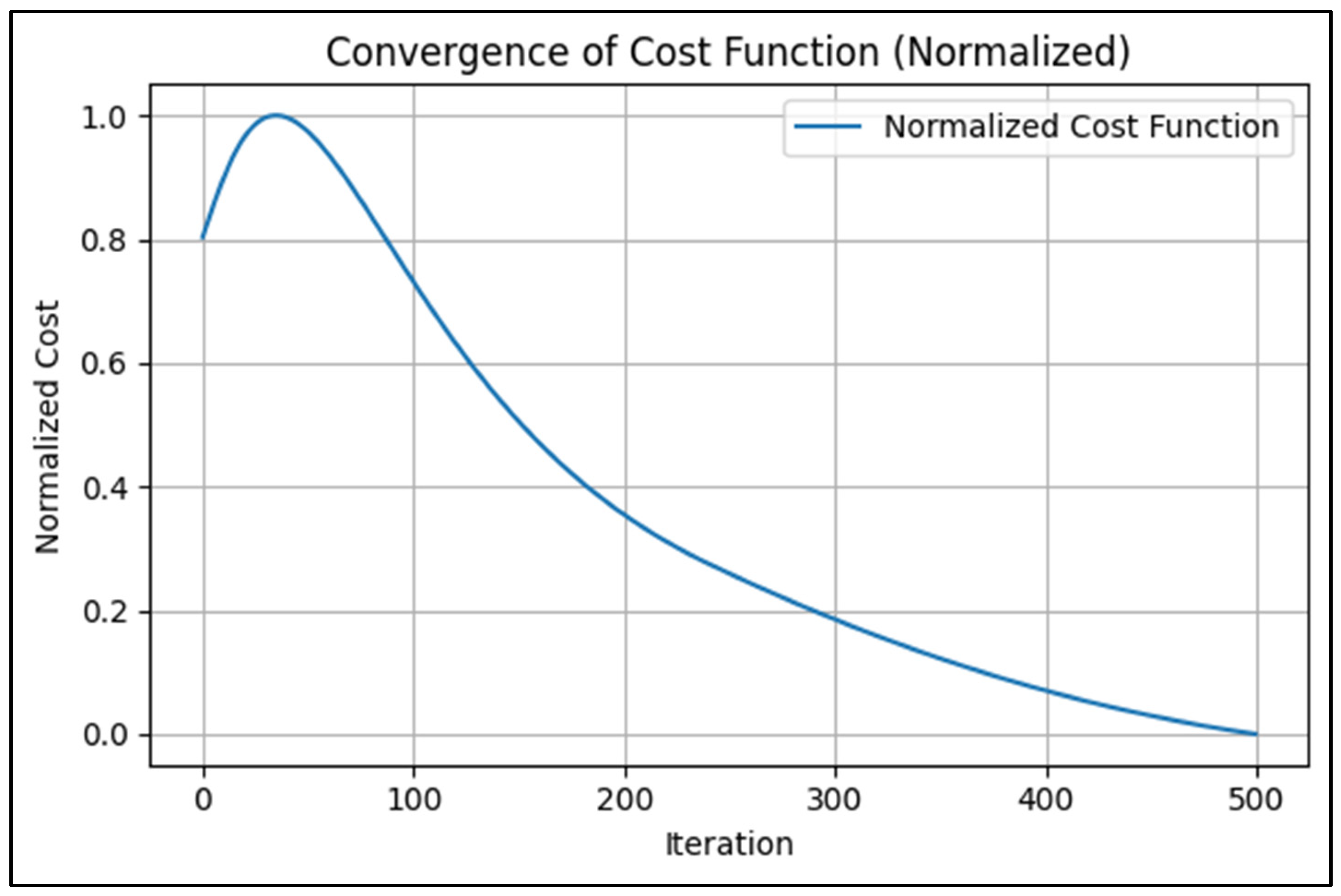
Each figure shows, for a given iteration step, the comparison between true and inverted model and their difference in percentage, for both velocity and resistivity models. Finally, Figure 6 shows the trend of the joint inversion cumulative cost function for the whole inversion run.
The joint inversion framework, with cross-gradient regularization, successfully recovers the three anomalous features present in both models and preserves their structural correspondence. Model errors range between 0 and ±20% and are caused mostly by the gaussian noise added to the synthetic data and the starting models.
This setup provides stable measurements and good depth sensitivity while minimizing sensitivity to near-surface heterogeneity.
As said earlier, the seismic/geoelectric layout used the same coordinates for source and receiver positions, allowing for a tight coupling between datasets in the joint inversion process. This common acquisition grid ensures that both datasets sample the same subsurface volume, which is essential for applying the cross-gradient constraint method in the joint inversion approach. Such a configuration is highly applicable in mineral exploration, where resolving both structural and compositional variations is crucial. The inclusion of a deep reflector (not visible in the figures) mimics typical scenarios found in hard rock geology and ore body detection.
The configuration and methodology employed in this simulation reflect conditions often encountered in mineral exploration campaigns, where high-resolution imaging of resistive (or conductive) and/or fast seismic anomalies is necessary to identify ore deposits, alteration zones, or fluid-filled fractures. The joint use of seismic and electrical methods enhances interpretability, especially when geophysical contrasts are subtle or ambiguous when using only a single technique. This simulated scenario represents a typical synthetic benchmark for subsurface prospecting in mineral-rich regions, especially in the early stages of exploration when drilling data is sparse.
4. Discussion: Benefits and Limitations
The proposed framework demonstrates a pathway for robust and adaptive joint inversion, capable of operating without tight manual supervision. In mineral exploration contexts, such an algorithm could be deployed to identify targets where complex lithological contrasts coexist. The integration of seismic and electrical data provides enhanced imaging capacity, and the algorithm's self-regulation reduces the need for fine-tuning, making it well-suited for automated prospecting platforms, drone-based surveys, or large-scale regional screening.
This preliminary synthetic validation provides a foundation for future applications on real datasets, potentially including magnetotellurics, gravity, or EM methods, all within the same self-aware computational framework. Of course, our proposed approach includes both benefits and limitation which can be summarized as following.
- Benefits:
- Improved accuracy: by jointly inverting seismic and resistivity data, the proposed method generates a more accurate and detailed model of the subsurface, which is particularly beneficial in mineral exploration.
- Self-aware learning: the integration of self-aware learning enables dynamic adjustments of hyper-parameters during the inversion process, improving convergence speed and model accuracy.
- Adaptability: the self-adjustment of hyperparameters ensures that the algorithm adapts to changing data characteristics, preventing overfitting and ensuring robust results.
- Flexibility: the method can be applied to a wide range of geophysical datasets and can incorporate additional geophysical data types in the future.
- Limitations
- Computational complexity: the joint inversion process, combined with self-aware learning, can be computationally intensive, particularly for large-scale 3D datasets.
- Noise sensitivity: while the self-aware learning mechanism helps prevent overfitting, extreme levels of noise in the data may still pose challenges.
- Limited real-world testing: the method was tested using synthetic data, and further validation with real-world datasets is needed to confirm its robustness in actual exploration scenarios.
5. Conclusions and Future Work
This preliminary study demonstrates the potential of geophysical joint inversion for subsurface characterization in mineral exploration, with an emphasis on the integration of seismic velocity and resistivity data. The proposed self-aware learning improves the accuracy and efficiency of the inversion process by dynamically adjusting the learning rate, other hyperparameters, and finally allowing for more robust and adaptive models.
Future work will focus on applying the method to real-world datasets to validate its performance in actual mineral exploration settings. Additionally, the methodology could be expanded to include other geophysical methods, such as magnetics or gravity, to further enhance subsurface characterization. Computational optimization techniques will also be explored to improve the scalability and efficiency of the algorithm for larger datasets.
Appendix: Self-Learning and Self-Aware Basic Mechanisms in the Joint Inversion Framework
A distinctive feature of this research is the integration of self-aware hyperparameter tuning and adaptive learning dynamics, inspired by concepts of metacognition and self-regulation. The joint inversion algorithm is designed to act as a semi-autonomous system that monitors its internal state and adjusts its behavior accordingly. Below, we outline key mechanisms that support this behavior and provide simplified Python code to illustrate critical aspects of the methodology. The full implementation is significantly more complex and includes dynamic adjustment of a wide range of hyperparameters beyond those shown here.
- 1.
- Self-Awareness in Hyperparameter Adaptation
The inversion process incorporates a feedback mechanism that adapts learning rates, specifically “alpha_v” for the velocity model and “alpha_r” for the resistivity model, based on the evolving data misfit. This is governed by the function “self_reflect”, which operates as a form of internal self-evaluation:
def self_reflect(alpha, grad, misfit):
norm = np.linalg.norm(misfit)
alpha *= 0.95 if norm < 0.5 else 1.05
alpha = np.clip(alpha, 1e-4, 0.1)
return alpha
This mechanism mimics a self-aware agent that adjusts its learning behavior in real time. When the misfit norm is small, the algorithm reduces its step size to avoid overshooting; when large, it increases the step to accelerate convergence. This balances caution and responsiveness in a self-regularized learning trajectory.
- 2.
- Adaptive Smoothing Inspired by Learning Maturation
The smoothing parameter “sigma_smooth”, applied to both models, evolves over the course of the inversion:
sigma_smooth = max(0.8, 2.0 - iteration / 200)
This decreasing function emulates the maturation of learning: early iterations apply stronger smoothing to stabilize updates and enforce regularity, while later stages permit finer structural detail as the model "gains confidence." This mechanism reflects a form of temporal awareness and stage-specific learning control.
- 3.
- Feedback-Driven Update with Cross-Domain Coupling
Each model update integrates three core components:
- A data-misfit gradient term,
- A spatial smoothing term, and
- A cross-gradient coupling constraint, cg, encouraging structural similarity across domains.
velocity_model -= alpha_v * grad_tt \
+ w_smooth_v * smoothing(velocity_model, sigma=sigma_smooth) \
+ beta * cg
resistivity_model -= alpha_r * grad_rho \
+ w_smooth_r * smoothing(resistivity_model, sigma=sigma_smooth) \
- beta * cg
Here, “beta” is the cross-gradient weight, and “w_smooth_v”, “w_smooth_r” are domain-specific smoothing weights. These coefficients govern the trade-off between fidelity, regularity, and structural coupling. Their values can also be made self-adjusting based on local curvature, data quality, or misfit evolution.
- 4.
- Domain-Specific Misfit Weights with Self-Tuning
In multi-domain joint inversion, the system can dynamically adjust the relative importance of different geophysical data types (e.g., seismic, electrical, gravimetric), using misfit weights “w_seis”, “w_elec”, “w_grav”, etc. A self-aware extension includes automatic adjustment of these weights to balance the contribution of each data type:
def adjust_misfit_weights(w, misfit):
scale = np.linalg.norm(misfit)
w *= 1.0 + 0.05 * np.sign(scale - target_level)
return np.clip(w, 0.01, 1.0)
This allows the system to upweight underperforming data domains or downweight noisy channels, providing data-adaptive fusion during inversion.
- 5.
- Adaptive Cross-Gradient Constraint
The coupling strength “beta” that governs the cross-gradient constraint can itself be self-regulated based on structural divergence between the velocity and resistivity models:
def update_beta(beta, cg_magnitude):
beta *= 1.05 if cg_magnitude > threshold else 0.95
return np.clip(beta, 0.01, 1.0)
This reflects the system’s internal awareness of consistency between domains and its desire to enforce similarity only when beneficial. If the models are naturally divergent (e.g., due to true physical contrasts), the constraint is relaxed.
- 6.
- Self-Monitoring and Visualization of Learning Progress
Throughout the optimization, the system monitors:
- The misfit curves across different domains,
- The evolution of key hyperparameters (alpha, beta, weights),
- The structural correlation between inverted models.
Visualization and logging are integrated as self-observation tools, enabling identification of instability, premature convergence, or imbalance in data-domain influence.

Table 1.
Summary of Self-Aware Mechanisms.
| Hyperparameter | Self-Adjustment Mechanism |
|---|---|
| Learning rates (alpha_v, alpha_r) | Adjusted based on misfit norm evolution |
| Smoothing factor (sigma_smooth) | Decreases over iterations to allow fine detail |
| Cross-gradient weight (beta) | Tuned based on structural similarity between models |
| Misfit weights (w_seis, w_elec, etc.) | Balanced according to relative misfit magnitudes |
| Smoothing weights (w_smooth_v, w_smooth_r) | Adjustable to control spatial coherence |
| Visualization frequency | Triggered adaptively by error dynamics or plateau detection |
These mechanisms form the foundation of a self-aware inversion system, capable of dynamically controlling its behavior through internal feedback loops. The result is an adaptive and resilient framework suited to real-world, multimodal geophysical challenges.
References
- Yilmaz, Ö., 2001. Seismic Data Analysis: Processing, Inversion, and Interpretation of Seismic Data. SEG Books.
- Nabighian, M.N., 2008. Electromagnetic Methods in Applied Geophysics: Applications, Part A and Part B. Society of Exploration Geophysicists.
- Aster, A., Borchers, B., and Thurber, C., 2003, Parameter estimation and inverse problems, Academic Press, New York.
- Backus, G., and Gilbert, F., 1967. Numerical applications of a formalism for geophysical inverse problems, Geophys. J. Royal Astron. Soc., 13, 247–276. [CrossRef]
- Vozoff, K, Jupp, D. L. B., 1975. Joint Inversion of Geophysical Data, Geophysical Journal International, Volume 42, Issue 3, September 1975, Pages 977–991. [CrossRef]
- Colombo, D., McNeice, G., Raterman, N., Turkoglu, E., Sandoval-Curiel, E., 2014. Massive integration of 3D EM, gravity and seismic data for deepwater subsalt imaging in the Red Sea. Exp. Abstracts, SEG 2014.
- Dell’Aversana, P., 2014. Integrated Geophysical Models: Combining Rock Physics with Seismic, Electromagnetic and Gravity Data. EAGE Publications.
- Haber, E. and Oldenburg, D., 1997. Joint Inversion: A Structural Approach, Inverse Problems, Vol. 13, No. 1, 1997, pp. 63-77. [CrossRef]
- Giampaolo, V., Dell’Aversana, P., Capozzoli, L., De Martino, G., Rizzo, E., 2021. Combining Multi-temporal Electric Resistivity Tomography and Predictive Algorithms for supporting aquifer monitoring and management. NSG2021 1st Conference on Hydrogeophysics, 2021.0(1).
- Giampaolo, V., Rizzo, E., Straface, S., Votta, M., 2011. Hydrogeophysics techniques for the characterization of a heterogeneous aquifer. Bollettino di Geofisica Teorica ed Applicata, 52, 595-606. [CrossRef]
- Günther, T., Rücker, C., Spitzer, K., 2006. Three–dimensional modeling and inversion of dc resistivity data incorporating topography–II Inversion. Geophysical Journal International, 166, 506–517. 44. [CrossRef]
- Dell‘Aversana, P., 2001. Integration of seismic, MT and gravity data in a thrust belt interpretation. First Break, Volume 19, Issue 6, Jun 2001. [CrossRef]
- Dell’Aversana P., 2024. An introduction to Self-Aware Deep Learning for medical imaging and diagnosis. Explor Digit Health Technol. 2024; 2:218–34. [CrossRef]
- Dell’Aversana, P., 2024. Enhancing Deep Learning and Computer Image Analysis in Petrography through Artificial Self-Awareness Mechanisms. Minerals 2024, 14, 247. [CrossRef]
- Dell'Aversana, P., 2024. Reservoir geophysical monitoring supported by artificial general intelligence and Q-Learning for oil production optimization. AIMS Geosciences, 2024, 10(3): 641-661. [CrossRef]
- Tarantola, A., 2005. Inverse Problem Theory and Methods for Model Parameter Estimation. SIAM. ISBN 978-0-89871-572-9.
- Boyd, S.P., Vandenberghe, L., 2004, Convex Optimization. Cambridge University Press. p. 129. ISBN 978-0-521-83378-3.
- Horst, R., Tuy, H., 1996, Global Optimization: Deterministic Approaches, Springer.
- Neumaier, A., 2004, Complete Search in Continuous Global Optimization and Constraint Satisfaction, pp. 271–369 in: Acta Numerica 2004 (A. Iserles, ed.), Cambridge University Press 2004.
- Raschka, S. and Mirjalili, V., 2017, Python Machine Learning: Machine Learning and Deep Learning with Python, scikit-learn, and TensorFlow, 2nd Edition, PACKT Books.
- Ravichandiran, S., 2020, Deep Reinforcement learning with Python, Packt Publishing.
- Dell’Aversana, P., 2022. Reinforcement learning in optimization problems. Applications to geophysical data inversion. AIMS Geosciences, 2022, 8(3): 488-502. [CrossRef]
- Dell’Aversana, P., 2023. Inversion of geophysical data supported by Reinforcement Learning. Bulletin of Geophysics and Oceanography, Vol. 64, n. 1, pp. 45-60; March 2023. [CrossRef]
- Dell’Aversana, P. A Biological-Inspired Deep Learning Framework for Big Data Mining and Automatic Classification in Geosciences. Minerals 2025, 15, 356. [CrossRef]
Figure 1.
Block diagram and key elements of the simultaneous joint inversion workflow combining multiple geophysical domains/models, here referred as A, B and C.
Figure 1.
Block diagram and key elements of the simultaneous joint inversion workflow combining multiple geophysical domains/models, here referred as A, B and C.
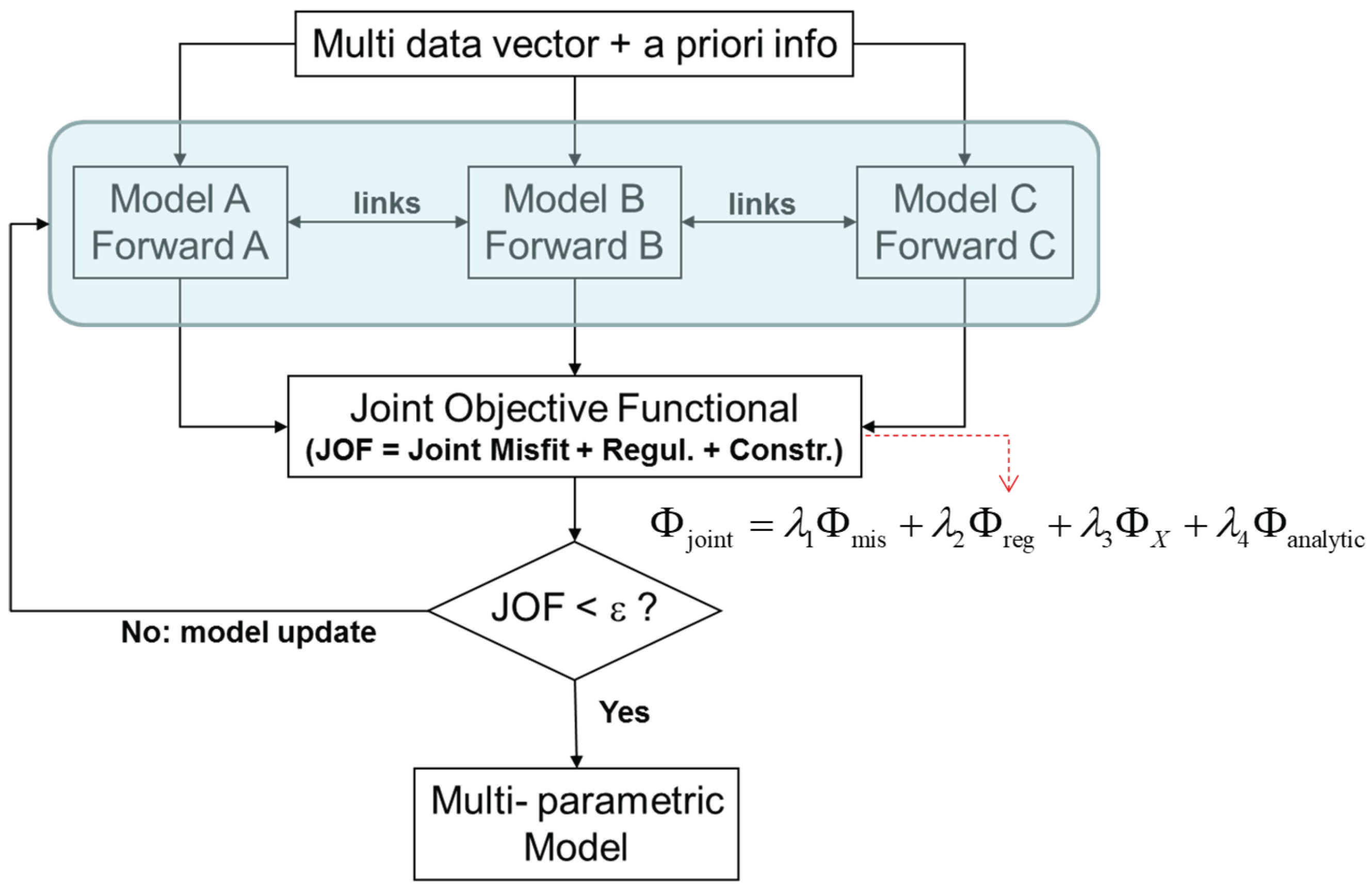
Figure 2.
True model, inverted model and differences (in %) for the seismic velocity distribution (top panels) and resistivity distribution (bottom panels) at iteration 0.
Figure 2.
True model, inverted model and differences (in %) for the seismic velocity distribution (top panels) and resistivity distribution (bottom panels) at iteration 0.
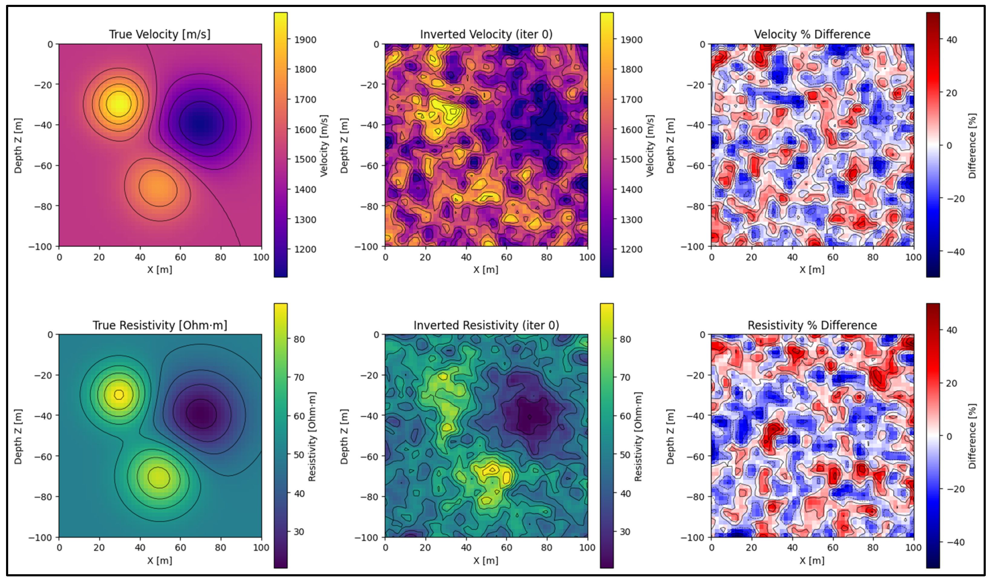
Figure 3.
True model, inverted model and differences (in %) for the seismic velocity distribution (top panels) and resistivity distribution (bottom panels) at iteration 50.
Figure 3.
True model, inverted model and differences (in %) for the seismic velocity distribution (top panels) and resistivity distribution (bottom panels) at iteration 50.
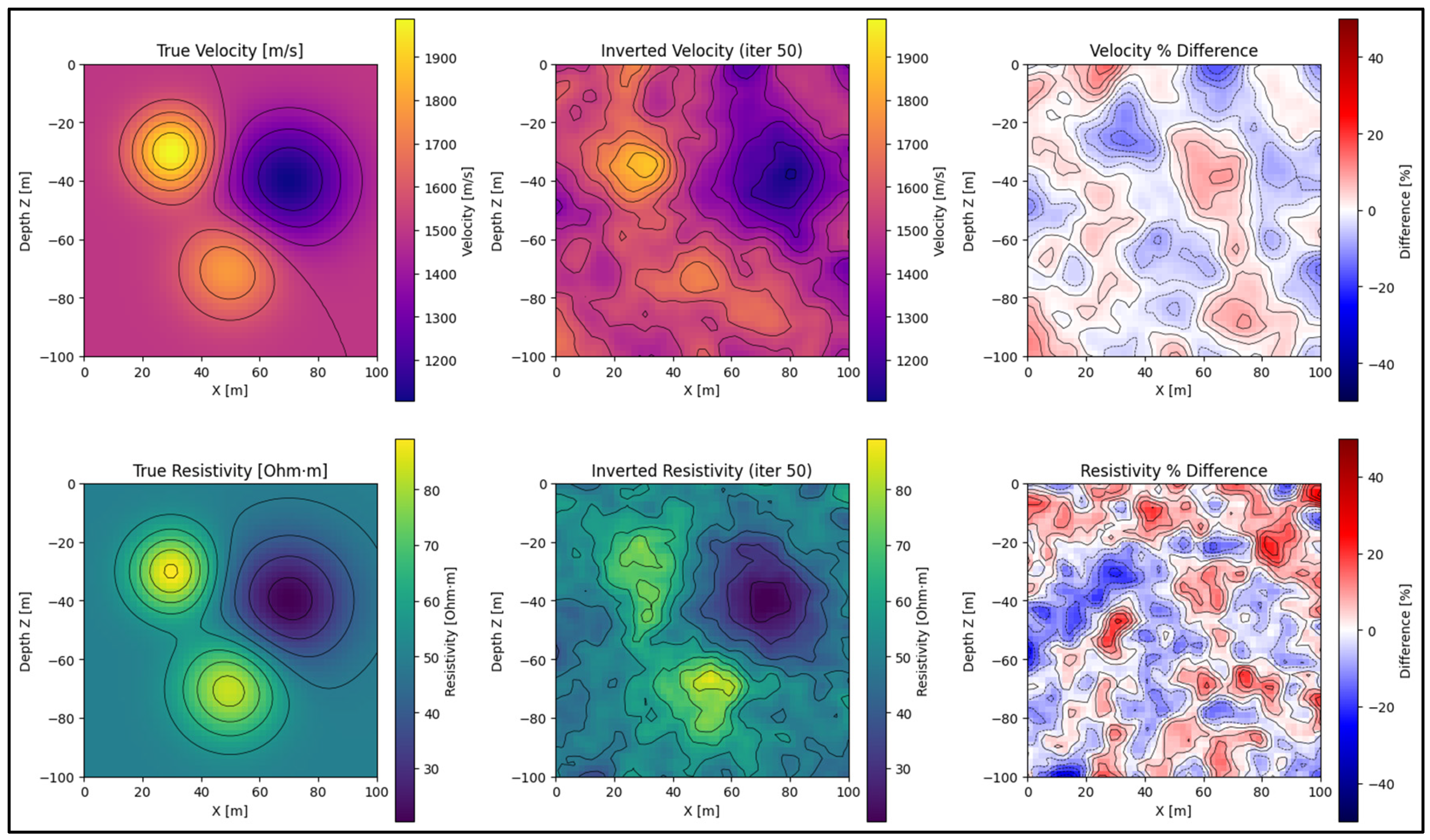
Figure 4.
True model, inverted model and differences (in %) for the seismic velocity distribution (top panels) and resistivity distribution (bottom panels) at iteration 200.
Figure 4.
True model, inverted model and differences (in %) for the seismic velocity distribution (top panels) and resistivity distribution (bottom panels) at iteration 200.
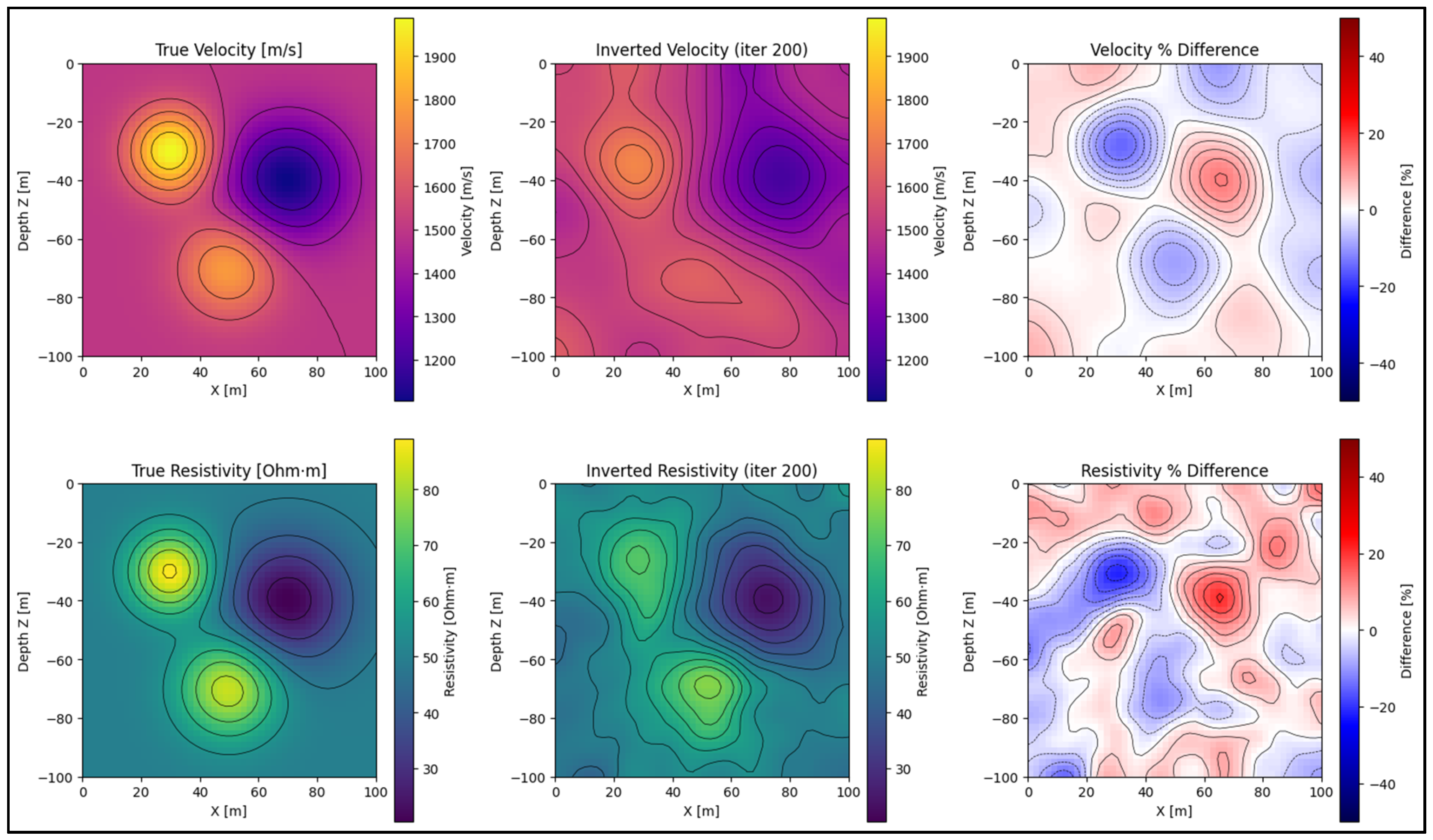
Figure 5.
True model, inverted model and differences (in %) for the seismic velocity distribution (top panels) and resistivity distribution (bottom panels) at iteration 499.
Figure 5.
True model, inverted model and differences (in %) for the seismic velocity distribution (top panels) and resistivity distribution (bottom panels) at iteration 499.
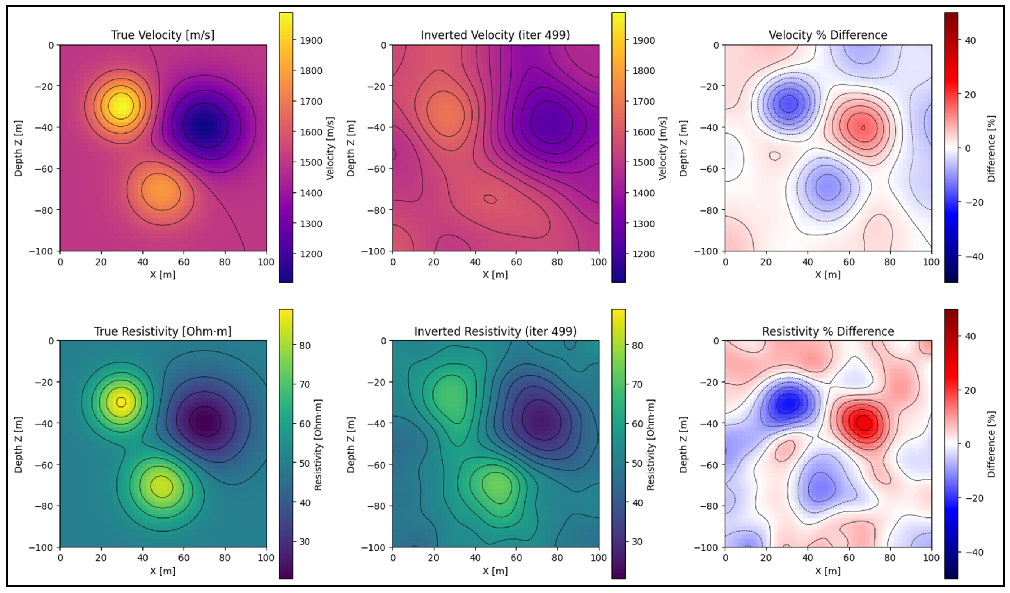
Figure 6.
Trend of the Joint Inversion cost function vs. iteration number.
Disclaimer/Publisher’s Note: The statements, opinions and data contained in all publications are solely those of the individual author(s) and contributor(s) and not of MDPI and/or the editor(s). MDPI and/or the editor(s) disclaim responsibility for any injury to people or property resulting from any ideas, methods, instructions or products referred to in the content. |
© 2025 by the authors. Licensee MDPI, Basel, Switzerland. This article is an open access article distributed under the terms and conditions of the Creative Commons Attribution (CC BY) license (http://creativecommons.org/licenses/by/4.0/).
Copyright: This open access article is published under a Creative Commons CC BY 4.0 license, which permit the free download, distribution, and reuse, provided that the author and preprint are cited in any reuse.


