
Submitted:
21 October 2025
Posted:
21 October 2025
You are already at the latest version
Abstract
The estimation of subsurface seismic velocities is fundamental in seismic data processing, as it enables the accurate positioning of reflections and diffractions within the subsurface. However, traditional methods often face challenges in scenarios characterized by strong velocity contrasts, blind zones, and complex geological structures, which limit the reliability of the resulting models. This study presents a seismic tomography approach based on neural networks. A total of 100,000 synthetic one-dimensional (1D) lithological models were randomly generated with increasing velocities and sharp contrasts. These models were spatially discretized into blocks, each assigned a specific velocity and density. Acoustic impedance and reflectivity profiles were derived from each model, and the reflectivity profiles were labeled according to their corresponding velocity models. The dataset was divided into training, validation, and testing subsets to develop and evaluate the model. The trained neural network accurately predicted velocity profiles from reflectivity data, even in cases involving strong velocity contrasts. The model exhibited strong generalization performance on unseen data, validating its robustness. This approach provides a fast and accurate alternative for estimating seismic velocity profiles, significantly reducing manual intervention and offering a reliable solution for subsurface characterization in complex geological environments.
Keywords:
tomography
; neural network
; seismic
1. Introduction
A foundational approach was presented by Aki [1,2], who inverted the travel times of acoustic plane waves through a regular grid to obtain a velocity distribution, thereby reducing the problem to a linear one. This work led to the development of seismic tomography techniques, which are used to simultaneously estimate velocity models and hypocenter locations. Despite its usefulness, tomography presents well-known limitations such as high-frequency ray tracing approximations, regularization effects, and smoothing constraints, all of which influence the fidelity of wave propagation modeling.
Classical seismic tomography methods require an initial subsurface velocity model, which is iteratively updated until a geologically interpretable solution is obtained. This initial model must incorporate prior geological information to constrain the range of possible velocity distributions and facilitate algorithm convergence. The process is based on the comparison between synthetic data generated by a model and field-observed data; from this comparison, an error is calculated, and the model parameters are adjusted to minimize it. This approach has significant limitations, including high dependence on the initial model, long computational times, and the possibility of non-unique solutions [3]. Furthermore, seismic data preprocessing, which involves critical steps such as signal filtering and first-arrival picking, can introduce errors that compromise the accuracy of the inversion results. Another challenge arises in regions with strong velocity contrasts, where modeling can be particularly difficult.
Neural networks have proven to be essential tools for velocity model estimation, as they can learn complex relationships between traveltimes and subsurface properties from synthetic data [4,5,6,7,8,9,10,11,12], which allow generating or complementing velocity models when field data are scarce or incomplete [13,15]. This approach reduces costs and development time by enabling the evaluation of multiple controlled scenarios without relying exclusively on field data . Although training requires computational resources, these are not as demanding compared to other methods such as Full Waveform Inversion (FWI) [4,11,14,16,17,18,19,20], and prediction is almost instantaneous [21] and low-cost, offering advantages over traditional iterative methods [5,16,17,22]. Another important aspect is generalization, as neural networks can adapt to geological conditions not explicitly represented in the training data, provided sufficiently large and diverse synthetic datasets are available [11,12,17,23]. Their fast inference and ability to capture complex nonlinear relationships enable the generation of precise, high-resolution velocity models [4,5,17].
In this study, we propose a neural network-based model, specifically a multilayer perceptron (MLP), which was developed and trained with synthetic data to obtain velocity models that account for strong velocity contrasts, multiples, and noise. Once trained, this approach enables fast model estimation with minimal preprocessing, reducing interpretation-related errors within the workflow, such as first-arrival picking, since only reflectivity profiles are required. Furthermore, the model demonstrates adequate generalization capability on data not used during training, making it a valuable alternative to methods based on full waveform inversion and other approaches that rely on initial models, which strongly influence the final velocity results. For these reasons, neural networks are established as a competitive alternative to classical seismic tomography methods, reinforcing and complementing the value of field data [16,18,24,25].
2. Materials and Methods
2.1. Input Data
When a P-wave with amplitude hits perpendicularly the j-interface that separates two media with different densities , and P- wave velocityVp, the reflectivity coefficient determines the amplitude of the reflected one like:
This reflectivity is also given by:
On the other hand, the seismic trace is a time series that results from the convolution of the wavelet with the reflectivity ,and added noise [26],
So, to recover the reflectivity attenuate first the noise and then apply the deconvolution [26].
Where is an inverse filter estimated by deterministic or statistical methods. Next, the seismic inversion infers the distribution of density and P and S wave velocity in the subsoil from the reflectivity. Because this research performs seismic inversion using neural networks, an introduction to this topic is included.
2.2. Multi-Layer Neural Network
In the following sections, we shall address two essential mechanisms of neural networks: feedforward propagation, responsible for transmitting the input information through the layers to produce the network’s output, and backward propagation, which enables the adjustment of the model parameters by minimizing the error through gradient-based optimization techniques.
2.2.1. Feedforward Propagation
Feedforward propagation constitutes the stage in which input information is systematically transmitted through the successive layers of the neural network. At each layer, the inputs are linearly combined with the corresponding weights and biases, followed by the application of an activation function. This procedure is repeated sequentially across the layers until the final output is obtained. The feedforward phase thereby establishes a direct mapping from the input space to the output space, providing the foundation for subsequent error evaluation and parameter optimization during the backward propagation stage. To elucidate this process in greater detail, it is instructive to first examine the formal structure of an artificial neuron and to describe how its mathematical formulation underpins the forward transmission of information within the network.
The Figure 1 shows the simplified neural network scheme [27] is the input data, in this case, is the reflectivity coefficients, and the neuron’s weights. is the dot product between x and w, and measures their similarity, with a maximum value when the two vectors are parallel, zero when they are orthogonal, and a negative value when they are antiparallel. is the activation function that represents the synaptic potential.
This scheme ([27,28]) allows modeling nonlinear problems by using layers with dozens of these simplified neurons. The neural network randomly establishes the weights of all the neurons, then when for the first neuron of the first hidden layer, and then will be evaluated by the activation function.
Activation functions serve a crucial role in defining the non-linear transformations within a neural network. Different choices of activation functions lead to different learning dynamics and model behaviors. Some of the most common activation functions, such as the sigmoid, hyperbolic tangent (tanh), and rectified linear unit (ReLU), can be seen in Figure 2.
These functions highlight the diversity of possible mappings that can be used depending on the design and requirements of the network architecture.
For the purpose of exemplification, we shall consider a hypothetical numerical case of a feedforward neural network. The architecture comprises three layers: an input layer, a hidden layer, and an output layer. Specifically, the input layer consists of three input units, the hidden layer is composed of four neurons, and the output layer likewise contains four neurons. This configuration, illustrated in Figure 3, will provide the framework for a detailed illustration of the computational procedures involved in both the forward and backward propagation stages.
The neural network randomly establishes the weights of all the neurons, so in the case of the first neuron of the first hidden layer, with function weights and inputs the activation function will evaluate and supply the output v. Figure 2 shows different activation functions and for the ELU one the output is . Similarly, the same procedure is applied to the other neurons in the layer. To perform this process more efficiently, the weights and biases of each layer are organized into matrices and vectors , respectively.
Here, and denote the weights and biases of the first hidden layer, while and correspond to the weights and biases of the output layer. The reflectivity for the model with velocity and density becomes
The vector is the input to each of the neurons of the hidden layer, generating as output the vector which becomes the input of each neuron of the output layer, to finally supply the output . The high mismatch between the output and velocity model indicates that the weights of the neural network must be updated to achieve a better prediction. The feedback method calculates the metric error between the obtained output and the desired . In Euclidean case, the error is given by equation 9:
This equation calculates the total error over the entire training dataset, by measuring the squared differences between the predicted velocities and the reference velocities .
2.2.2. Backforward Propagation
The backpropagation process is the fundamental mechanism by which a neural network adjusts its internal parameters to minimize the loss function. After the forward propagation phase, during which the model output is computed, the discrepancy between the predicted and reference outputs is propagated backward through the network layers. In this process, the partial gradients of the loss function with respect to the weights are computed, enabling parameter updates via an optimization algorithm, typically based on gradient descent. This iterative procedure allows the neural network to progressively improve its generalization capacity and predictive accuracy.
The equation 10 corresponds to the application of the chain rule in the calculation of the gradient during the learning process of a neural network.
This expression illustrates how the total error, , varies with respect to a specific weight w. The derivation through partial derivatives reveals the sequential dependence among the variables: first, how the error changes with the predicted output ; second, how this output depends on the internal variable , typically defined as the linear combination of inputs and weights; and finally, how this internal variable is directly influenced by the weight w. This chain of derivatives forms the core of the backpropagation algorithm, as it enables the precise computation of each weight’s contribution to the total error. Now, each term in this expression will be derived
The equation 11 shows the explicit calculation of the first term in the chain rule. Starting from the squared error function , the derivative with respect to the predicted output is computed as:
This result shows that the error gradient is directly governed by the difference between the predicted and reference values. In other words, the derivative quantifies the rate at which the total error changes as the predicted output deviates from the true target .
We now proceed to analytically estimate the second term of the chain rule, . The value of depends on the choice of activation function used in the neuron. As an example, the sigmoid activation function is considered (equation 12) here in order to show the analytical derivation:
By differentiating this expression with respect to , we obtain the next equation 13:
Finally, rewriting the derivative in terms of the predicted output itself yields:
To complete the chain rule, we now consider the third term, . The internal variable is defined in equation 15 as the linear combination of the input (or hidden unit value) with the corresponding weight w, plus the bias term b:
Taking the derivative of this expression with respect to the weight w, we obtain
which corresponds to equation 16. This result indicates that the sensitivity of the internal variable with respect to the weight is directly given by the input (or hidden activation) . In other words, the gradient flowing back through this connection is proportional to the value that was propagated forward during the feedforward phase.
Finally, by substituting Equations 11, 14, and 16 into Equation 10, the derivative of the total error with respect to the weight, , is obtained. This expression is used in Equation 17, which defines the update rule for the weights w during the learning process.
As shown in Equation 10, the change in each weight is proportional to the negative gradient of the error function with respect to that weight, scaled by the learning rate . This formulation corresponds to the standard gradient descent rule, which ensures that the weights are updated in the direction that minimizes the total error of the network. The gradient of the total error with respect to the bias can be expressed, in analogy to the weight case, as:
which mirrors the chain rule formulation used for the weights. The main difference appears in the last term of the derivative. While for the weight the dependence of is given by equation 16, for the bias we obtain:
This shows that the backpropagation update rule for the bias follows the same structure as that of the weights (see Equation 19), but with a constant contribution in the last term of the chain rule:
3. Methodology
This study applies neural networks to reflectivity profiles generated from randomly constructed velocity and density models. In this approach, the reflectivity profiles are used as input data, while the velocity profiles constitute the target variable. The algorithm employs the reflectivity profile because it is independent of the seismic source, as it can be obtained through a deconvolution process that removes the seismic wavelet from the seismogram.
A total of five-layer models were generated using ray tracing, each layer exhibiting local variations in density and velocity (see Figure 3a). The models extend to a depth of , with layers where density and P-wave velocity vary randomly between 1600 and , and between 1500 and , respectively.
The domain is discretized into 50 blocks of each, establishing the spatial resolution (see Figure 4).
Equation 2 computes the reflectivity profile for each of the models, as illustrated in Figure 5. Subsequently, the reflectivity profile of each model is used as the input to the neural network, which in turn outputs the corresponding velocity model associated with that profile. Figure 6 presents the schematic diagram of a multilayer neural network, where the reflectivity serves as the input and the resulting velocity profile is provided as the output.
The dataset was partitioned into three subsets: training (70%), validation (15%), and testing (15%). The training subset was employed to fit the neural network models, while the validation subset was used to guide model selection and fine-tuning of hyperparameters. The testing subset was reserved for evaluating the final model performance on previously unseen data, thereby providing an unbiased assessment of its generalization capability.
Figure 6 illustrates the flow of data through the neural network during the initial iteration of the training process. Subsequently, the predicted velocity of the network is compared with the reference velocity profile to compute the prediction error, which is then used to update the model parameters during the backpropagation stage.
The optimization of the neural network architecture was conducted using the Keras Tuner framework. Initially, the hyperparameter search space was systematically defined, including the number of hidden layers, the number of units per layer, the choice of activation functions, and regularization strategies such as dropout. The training set was used iteratively by the tuner to explore candidate architectures, while the validation set informed the selection of the most appropriate configuration. Upon identification of the optimal architecture and hyperparameters, the final model was trained and subsequently evaluated on the testing set to assess its predictive accuracy and generalization performance.
4. Analysis of Results and Discussions
The Keras Tuner optimization process identified an optimal neural network architecture, which is summarized in Table 1. This table details the configuration of each layer, including the number of neurons, the activation functions employed, and any regularization techniques applied, providing a comprehensive overview of the model selected through the hyperparameter tuning procedure.
The algorithm run included 100 epochs and the MAE optimization function (Mean Absolute Error), the ADAM optimizer with a learning rate, the MAE metrics, and the MSE (Mean Square Error). With the architecture of Table 1, the network trained the model, including 1871026 parameters.
The Figure 7 illustrates the performance of a predictive velocity model using training and validation metrics, organized into subplots (a), (b), and two scatter plots in (c). Subplot (a) shows the evolution of the Mean Absolute Error (MAE) over 30 epochs. MAE decreases rapidly in the first 10 epochs and stabilizes around 180 after epoch 20. The close alignment between training and validation curves indicates that the model fits the training data well while maintaining good generalization to unseen data. Subplot (b) presents the Mean Squared Error (MSE), exhibiting a similar trend: rapid initial decrease and stabilization after 15-20 epochs. The minimal gap between training and validation reinforces the model’s generalization capability.
The scatter plots in (c) compare predicted versus reference velocities, reporting and , MAE -139 , RMSE 180-184 , and MAPE . The red diagonal line represents the ideal vs , and the concentration of points near this line indicates high prediction accuracy. The color scale, reflecting absolute error, shows that larger errors are rare and mostly occur at extreme velocities.
Overall, the model demonstrates robust performance, with low errors, high correlation with reference data, and stable convergence across epochs. The similarity between training and validation metrics further indicates that there is no evidence of overfitting.
Figure 8.
Comparison of velocity profiles between reference models and predicted model. There are 50 blocks, and each block is 100 m, for a maximum depth of 5000 m.
Figure 8.
Comparison of velocity profiles between reference models and predicted model. There are 50 blocks, and each block is 100 m, for a maximum depth of 5000 m.
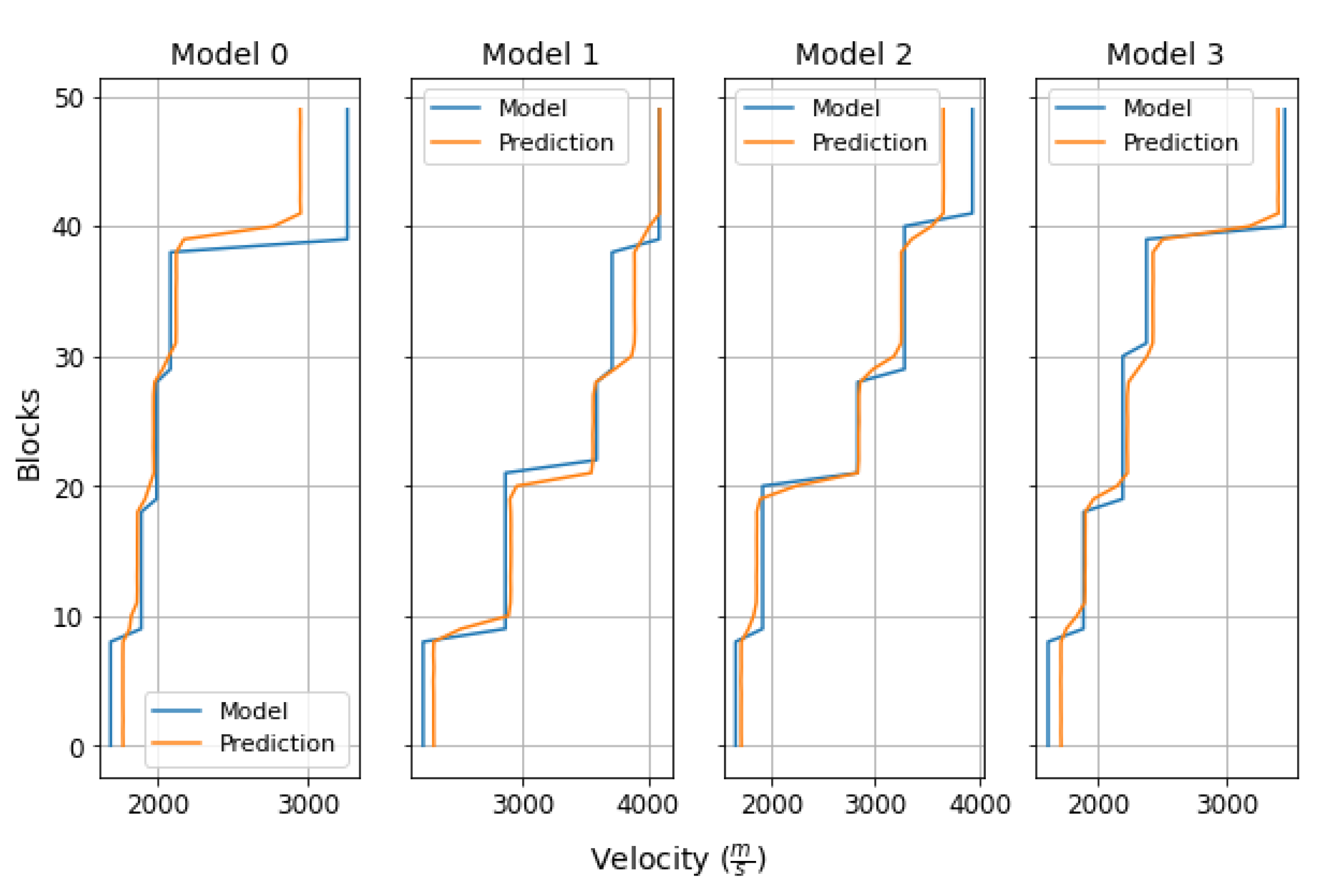
The plot shows the velocity profiles of four different models (Model 0 to Model 3), comparing the reference values (blue lines) with the model predictions (orange lines). Overall, the predictions closely follow the trends of the original models, capturing the jumps and variations in velocity across the different layers. Small deviations are observed in some intermediate layers, particularly in Model 0 and Model 1, where the predictions slightly under- or overestimate the velocity. Despite these minor differences, the overall agreement is high, indicating that the predictive method is robust and accurately reproduces the velocity profiles of the reference models.
5. Discussion
A multilayer perceptron model, trained with synthetic data, is presented, demonstrating adequate performance supported by consistent metrics in velocity profile estimation. The model is capable of reproducing both smooth and abrupt velocity changes, allowing for the identification of potential lithological transitions and providing estimates close to the reference values. It is important to note that the only preprocessing required is deconvolution, as the neural network receives the full reflectivity profile directly as input. This profile includes multiples and noise, demonstrating the model’s ability to handle complex data without the need for additional filtering. By requiring minimal preprocessing, data manipulation is reduced, thereby decreasing the potential for errors during data preparation. While synthetic data are approximations of the data that could be acquired in the field, they can serve as a useful complement for generating or augmenting datasets, particularly when field data are incomplete or unavailable, which is common in geophysics. This approach can be particularly useful in seismic inversion processes, since once the networks are trained, predictive models can be generated and inversion can be performed in significantly reduced times, optimizing workflows in geophysical studies.
The results obtained in this study demonstrate that the predictive velocity model achieves robust and stable performance. After the first twenty epochs, the mean absolute error stabilized at approximately , accompanied by a close agreement between training and validation sets. The mean squared error exhibited a similar trend, confirming the model’s ability to generalize beyond the training data. Overall, the performance indicators— values above , a MAE of about 138–, RMSE in the range of 180–, and MAPE of —highlight both the accuracy achieved and the consistency of the predictions. These outcomes indicate that the proposed approach maintains low discrepancies across training, validation, and test sets, ensuring reliability in the estimation of subsurface properties.
The strength of these metrics is directly linked to advantages previously recognized in neural network models trained with synthetic datasets. Chief among these is the reduction in cost and development time, since generating controlled scenarios makes it possible to test multiple configurations without relying on expensive field campaigns [4,5,11,12]. Although the training phase requires significant computational resources, the subsequent prediction stage is nearly instantaneous and incurs negligible cost, placing this approach at a clear advantage over conventional iterative procedures [5,16,17,22].
Another notable aspect is the model’s ability to generalize, as shown by its adaptability to acquisition settings and geological conditions not explicitly represented in the training data, provided that a sufficiently large and diverse synthetic dataset is available [11,12,17]. This property strengthens the applicability of the method in real-world scenarios, where geological variability is a persistent challenge.
Inference speed further distinguishes this approach. Unlike traditional inversion methods, deep learning models produce immediate results once training is complete [5,16,17,22], making them well suited for field exploration and real-time monitoring. Complementarily, the ability to capture highly nonlinear relationships between traveltimes and subsurface properties enhances the fidelity of the models and enables more accurate characterization of complex geological structures [5,17].
The methodological framework presented here is both flexible and scalable, allowing it to be adapted to different levels of resolution and to be integrated with complementary geophysical information. Taken together, these characteristics validate the relevance of the proposed approach and position it as a competitive alternative to classical seismic tomography methods, which face inherent limitations [16,18,24,25].
Author Contributions
Conceptualization, A.D. and L.M.; methodology, A.D. and L.M; software, A.D. and L.M; validation, A.D. and L.M.; formal analysis, A.D. and L.M; investigation, A.D. and L.M; resources, A.D. and L.M; data curation, A.D. and L.M; writing—original draft preparation, A.D. and L.M; writing—review and editing, A.D. and L.M; visualization, A.D. and L.M.; supervision, A.D. and L.M; project administration, A.D. and L.M; funding acquisition, A.D. and L.M. All authors have read and agreed to the published version of the manuscript.
Funding
This research was funded by Universidad Nacional de Colombia and Fundación Universitaria Politécnico Grancolombiano. The Article Processing Charge (APC) was also funded by Universidad Nacional de Colombia and Fundación Universitaria Politécnico Grancolombiano.
Data Availability Statement
The dataset used in this study ara available at the repository https://drive.google.com/file/d/1xhieRdN6wLf9ei7CNdwePPWkEbqV53kp/view?usp=sharing.
Conflicts of Interest
The authors declare no conflicts of interest.
References
- Aki, K.; Christoffersson, A.; Husebye, E.S. Determination of the three-dimensional seismic structure of the lithosphere. J. Geophys. Res. 1977, 82, 277–296. [CrossRef]
- Aki, K.; Lee, W.H.K. Determination of three-dimensional velocity anomalies under a seismic array using first P arrival times from local earthquakes: 1. A homogeneous initial model. J. Geophys. Res. 1976, 81, 4381–4399. [CrossRef]
- Tarantola, A. Inverse Problem Theory and Methods for Model Parameter Estimation; Society for Industrial and Applied Mathematics: Philadelphia, PA, USA, 2005. [CrossRef]
- Yang, F.; Ma, J. Deep-learning inversion: A next generation seismic velocity-model building method. arXiv 2019, arXiv:1902.06267. Available online: https://arxiv.org/abs/1902.06267.
- Araya, M.; Jennings, J.; Adler, A.; Dahlke, T. Deep-learning tomography. Lead. Edge 2018, 37, 58–66. [CrossRef]
- Araya-Polo, M.; Farris, S.; Florez, M. Deep learning-driven velocity model building workflow. Lead. Edge 2019, 38, 872a1–872a9. [CrossRef]
- Adler, A.; Araya-Polo, M.; Poggio, T. Deep learning for seismic inverse problems: Toward the acceleration of geophysical analysis workflows. IEEE Signal Process. Mag. 2021, 38, 89–119. [CrossRef]
- Wang, W.; Yang, F.; Ma, J. Velocity model building with a modified fully convolutional network. In Proceedings of the SEG Technical Program Expanded Abstracts, Anaheim, CA, USA, 14–19 October 2018; Society of Exploration Geophysicists: Tulsa, OK, USA, 2018; pp. 2086–2090. Available online: https://library.seg.org/doi/abs/10.1190/segam2018-2997566.1 (accessed on Day Month Year).
- Das, V.; Pollack, A.; Wollner, U.; Mukerji, T. Convolutional neural network for seismic impedance inversion. Geophysics 2019, 84(6), R869–R880.
- Duque, L.; Gutierrez, G.; Arias, C.; Rüger, A.; Jaramillo, H. Automated velocity estimation by deep learning based seismic-to-velocity mapping. In Proceedings of the EAGE Annual Meeting, London, UK, 3–6 June 2019; Volume 2019, No. 1, pp. 1–5. [CrossRef]
- Mousavi, S.M.; Beroza, G.; Mukerji, T.; Rasht-Behesht, M. Applications of Deep Neural Networks in Exploration Seismology: a technical survey. GEOPHYSICS 2024, 89, 1–93. [CrossRef]
- Ren, Y.; Nie, L.; Yang, S.; Jiang, P.; Chen, Y. Building Complex Seismic Velocity Models for Deep Learning Inversion. IEEE Access 2021, PP, 1–1. [CrossRef]
- Waheed, U.B.; Alkhalifah, T.; Haghighat, E.; Song, C.; Virieux, J. PINNtomo: Seismic tomography using physics-informed neural networks. arXiv 2021, arXiv:2104.01588. Available online: https://arxiv.org/abs/2104.01588.
- Liu, Y.; Dong, L.; Yang, J. Influence of wave front healing on seismic tomography. In Proceedings of the SEG Technical Program Expanded Abstracts, Denver, CO, USA, 17–22 October 2010; pp. 4257–4262. [CrossRef]
- Muller, A.P.O.; Bom, C.R.; Costa, J.C.; Klatt, M.; Faria, E.L.; dos Santos Silva, B.; de Albuquerque, M.P.; de Albuquerque, M.P. Deep-Tomography: Iterative velocity model building with deep learning. Geophys. J. Int. 2022, 232, 975–989. [CrossRef]
- Moseley, B.; Nissen-Meyer, T.; Markham, A. Deep learning for fast simulation of seismic waves in complex media. Solid Earth 2020, 11(4), 1527–1549. [CrossRef]
- Phan, S.D.T. Machine Learning Algorithms for Solving Some Seismic Inversion Challenges. Ph.D. Dissertation, The University of Texas at Austin, Austin, TX, USA, 2021. Available online: https://repositories.lib.utexas.edu/items/74427f6f-7f2d-4e9a-83ef-5a1438c61f4c (accessed on Day Month Year).
- Li, F.; Guo, Z.; Pan, X.; Liu, J.; Wang, Y.; Gao, D. Deep Learning with Adaptive Attention for Seismic Velocity Inversion. Remote Sensing 2022, 14(15), 3810. [CrossRef]
- Virieux, J.; Operto, S. An overview of full-waveform inversion in exploration geophysics. Geophysics 2009, 74(6), WCC1–WCC26. [CrossRef]
- Virieux, J.; Brossier, R.; Métivier, L.; Etienne, V.; Operto, S. Challenges in the full waveform inversion regarding data, model and optimisation. In Proceedings of the 74th EAGE Conference and Exhibition—Workshops, Copenhagen, Denmark, 4–7 June 2012.
- Fu, H.; Zhang, Y.; Ma, M. Seismic waveform inversion using a neural network-based forward. Journal of Physics: Conference Series, 1324(1), 012043, IOP Publishing, October 2019. [CrossRef]
- Parasyris, A.; Stankovic, L.; Stankovic, V. Synthetic Data Generation for Deep Learning-Based Inversion for Velocity Model Building. Remote Sensing 2023, 15(11), 2901. [CrossRef]
- Fabien-Ouellet, G.; Sarkar, R. Seismic velocity estimation: A deep recurrent neural-network approach. Geophysics 2020, 85, U21–U29. [CrossRef]
- Serlenga, V.; Stabile, T.A. How do Local Earthquake Tomography and Inverted Dataset Affect Earthquake Locations? The Case Study of High Agri Valley (Southern Italy). Geomatics, Natural Hazards and Risk 2018, 10(1), 49–78. [CrossRef]
- Moghadas, D. One-Dimensional Deep Learning Inversion of Electromagnetic Induction Data Using Convolutional Neural Network. Geophysical Journal International 2020, 222(1), 247–259. [CrossRef]
- Yilmaz, O. Seismic Data Analysis; Society of Exploration Geophysicists: Tulsa, OK, USA, 2001. [CrossRef]
- Rosenblatt, F. The perceptron: a probabilistic model for information storage and organization in the brain. Psychological Review 1958, 65(6), 386–408. Available online: https://api.semanticscholar.org/CorpusID:12781225 (accessed on Day Month Year).
- McCulloch, W.S.; Pitts, W. A logical calculus of the ideas immanent in nervous activity. The Bulletin of Mathematical Biophysics 1943, 5(4), 115–133. [CrossRef]
Figure 1.
Simplified neural network scheme.
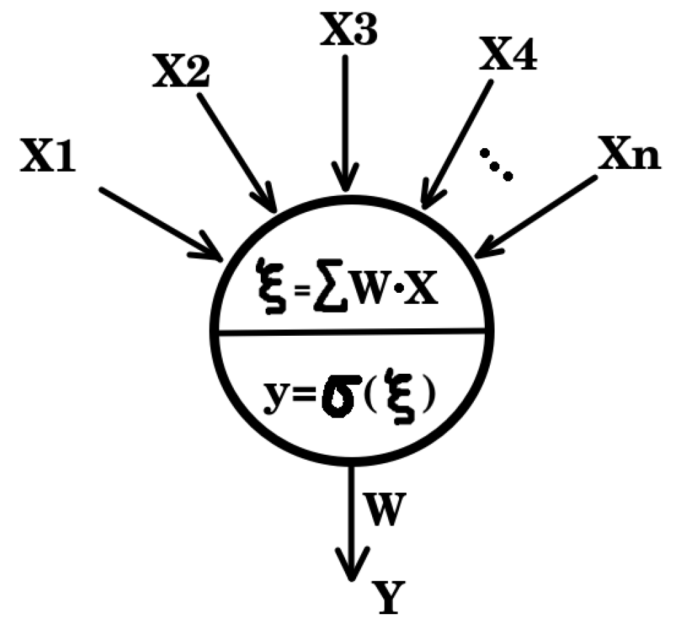
Figure 2.
Some activation functions commonly used in neural networks: Sigmoid, Tanh, ReLU, Leaky ReLU, and ELU. Each function defines a different nonlinear transformation that affects the gradient flow and the ability of the model to learn complex patterns.
Figure 2.
Some activation functions commonly used in neural networks: Sigmoid, Tanh, ReLU, Leaky ReLU, and ELU. Each function defines a different nonlinear transformation that affects the gradient flow and the ability of the model to learn complex patterns.

Figure 3.
Diagram explaining the feedforward in the MLP (Perceptron Multilayer) architecture.
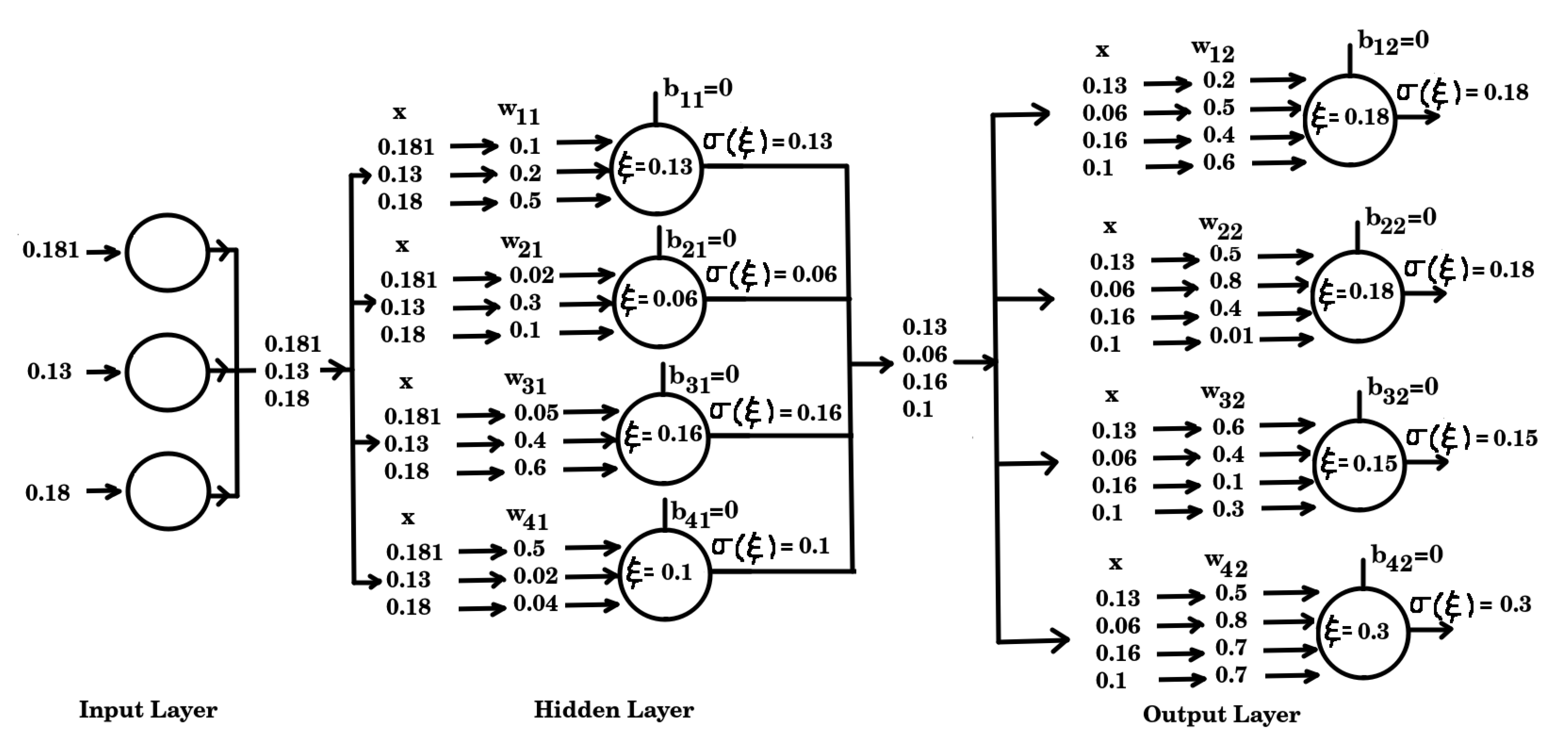
Figure 4.
a. Geological model of plane-parallel layers. b. The reflectivity of a geological model, where the yellow color highlights the strongest changes.
Figure 4.
a. Geological model of plane-parallel layers. b. The reflectivity of a geological model, where the yellow color highlights the strongest changes.
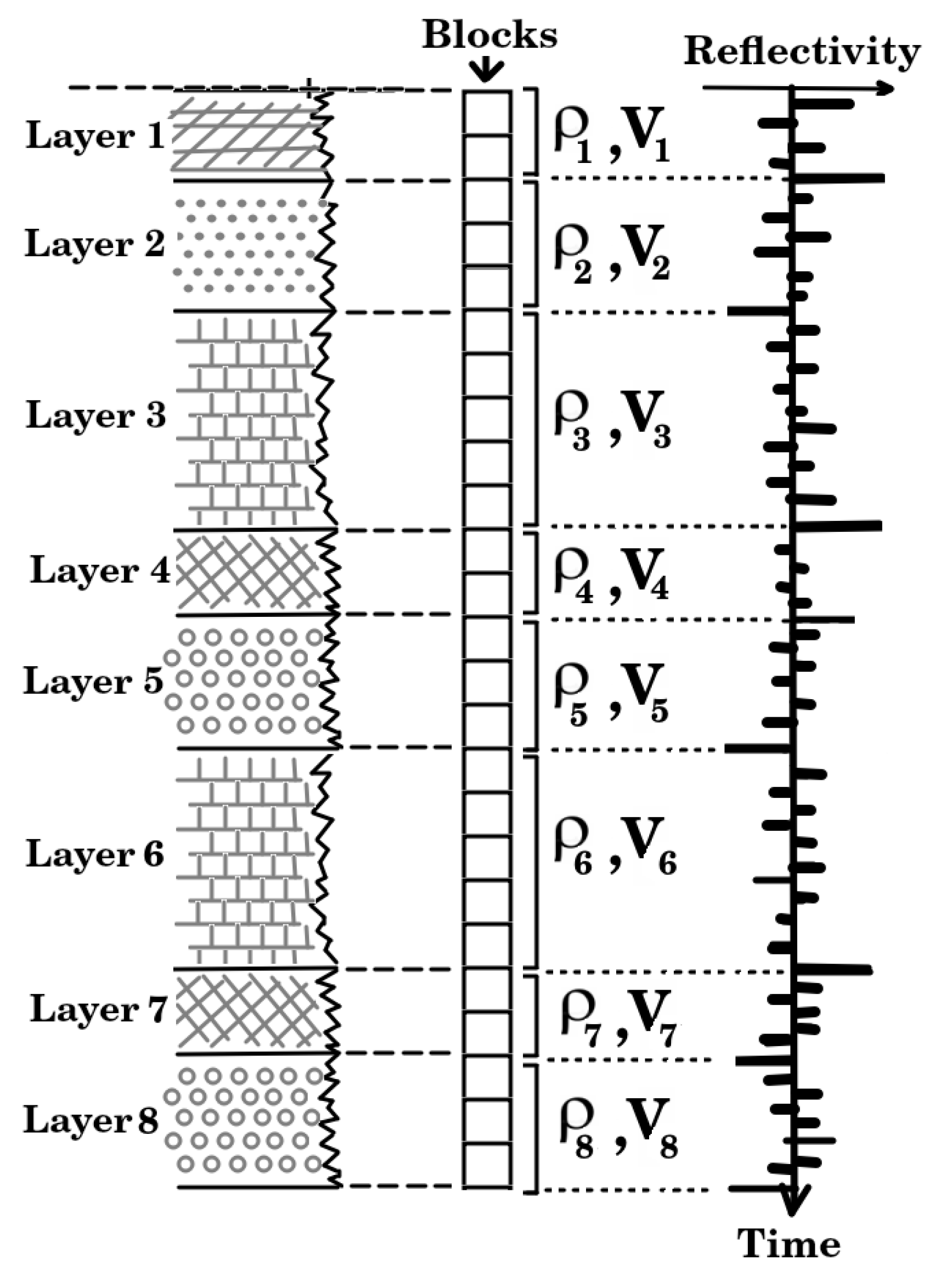
Figure 5.
Two reflectivity profiles corresponding to two randomly selected models.
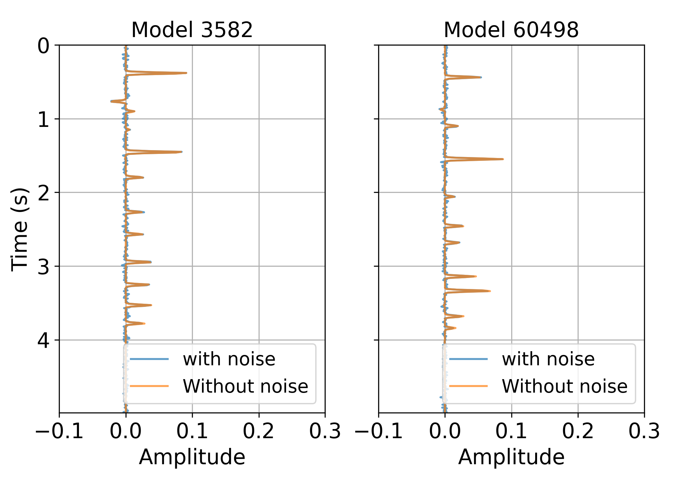
Figure 6.
Multilayer Neural network with the reflectivity as input and the P wave velocity as output.
Figure 6.
Multilayer Neural network with the reflectivity as input and the P wave velocity as output.
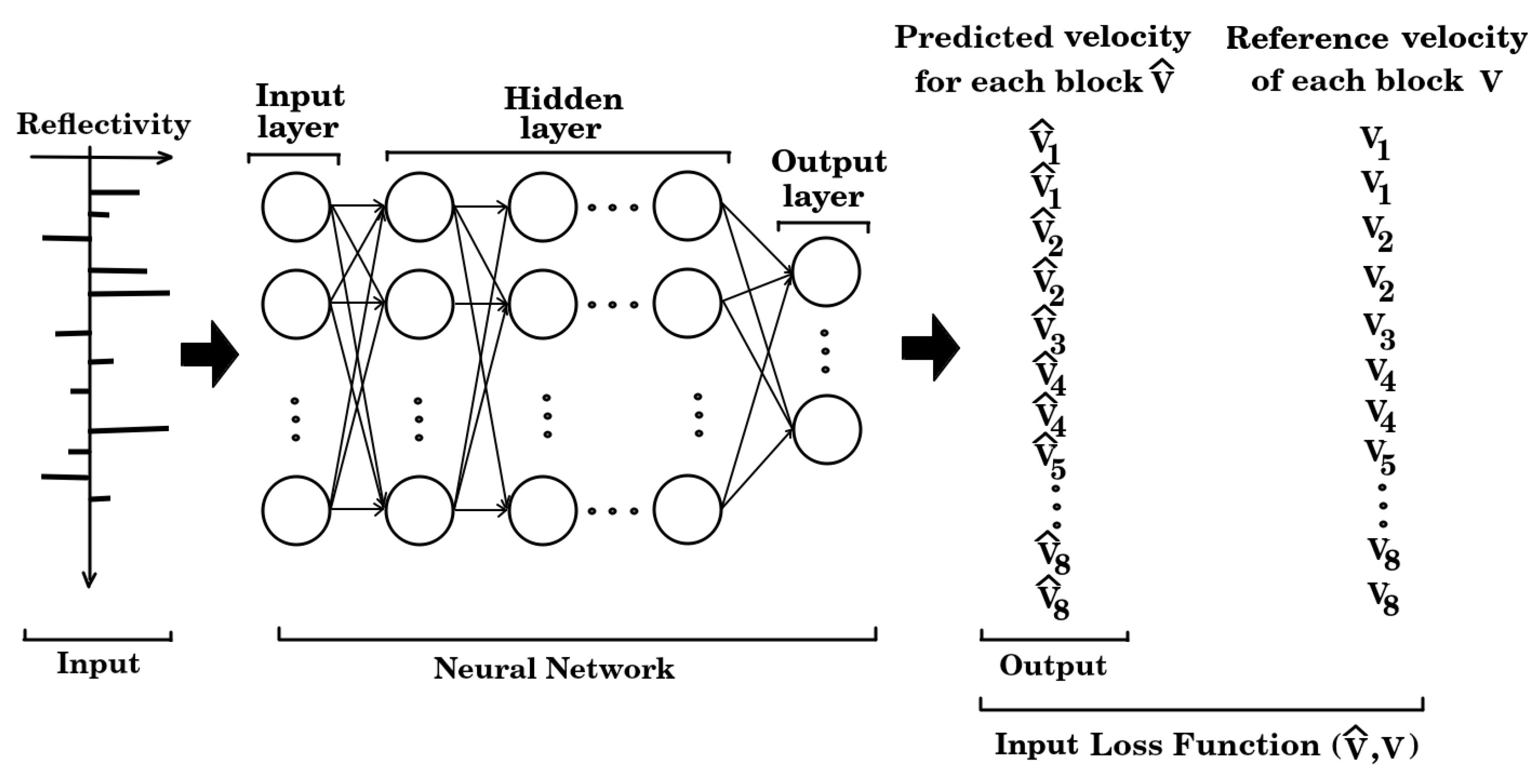
Figure 7.
This is a wide figure. Schemes follow the same formatting. If there are multiple panels, they should be listed as: (a) MAE curves achieved during training and validation of the neural network. (b) Cross plot of velocity model and predicted velocity. (c) Velocity model prediction for four random reflectivity profiles. (d) Description of what is contained in the fourth panel. Figures should be placed in the main text near to the first time they are cited. A caption on a single line should be centered.
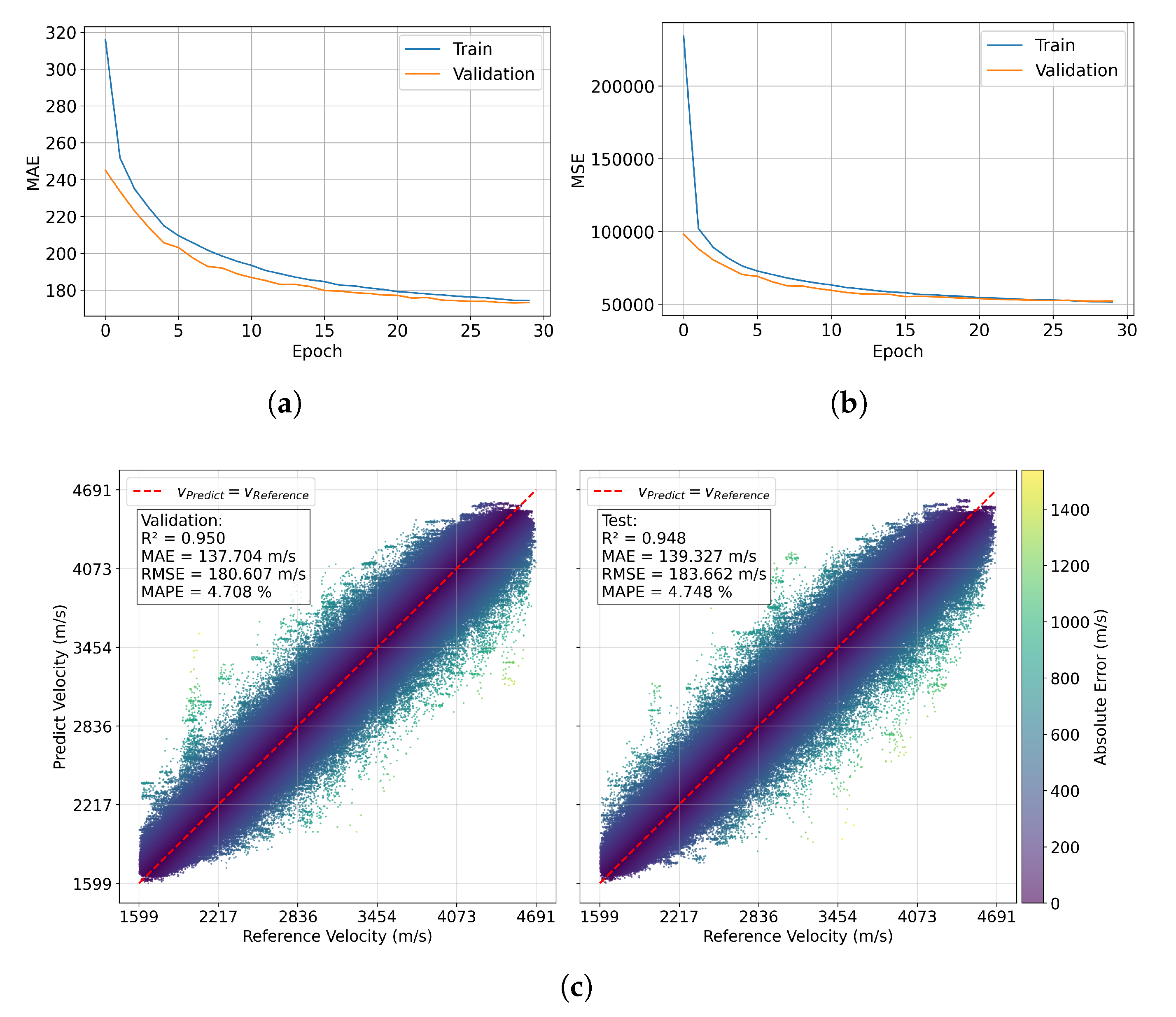

Table 1.
Table of the architecture found by Keras Tuner.
| Layer | Type and number of neurons | Hiperparameters |
|---|---|---|
| 1 | Dense(650) | Activation function ELU |
| 2 | Dense(650) | Activation function ELU |
| 3 | Dense(650) | Activation function ELU |
| 4 | Dropout | Factor 0.19 |
| 5 | Dense(750) | Activation function ELU |
| 6 | Dropout | Factor 0.26 |
| 7 | Dense(450) | Activation function ELU |
| 8 | Dropout | Factor 0.26 |
| 9 | Dense(50) | Activation function ELU |
Disclaimer/Publisher’s Note: The statements, opinions and data contained in all publications are solely those of the individual author(s) and contributor(s) and not of MDPI and/or the editor(s). MDPI and/or the editor(s) disclaim responsibility for any injury to people or property resulting from any ideas, methods, instructions or products referred to in the content. |
© 2025 by the authors. Licensee MDPI, Basel, Switzerland. This article is an open access article distributed under the terms and conditions of the Creative Commons Attribution (CC BY) license (http://creativecommons.org/licenses/by/4.0/).
Copyright: This open access article is published under a Creative Commons CC BY 4.0 license, which permit the free download, distribution, and reuse, provided that the author and preprint are cited in any reuse.


