Submitted:
14 May 2025
Posted:
14 May 2025
You are already at the latest version
Abstract
The H-index is a widely recognized centrality measure for nodes in symmetric networks, defined as the maximum number of neighbors with degrees equal to or greater than the node’s own degree. However, this metric underestimates the structural influence of "weak nodes" – low-degree nodes connected to high-degree hubs – that often serve as critical connectors in network topology. To address this limitation, we propose the Hα-index, which generalizes the H-index by considering the maximum number of neighbors with degrees at least α times the node’s degree, where α≥1. Based on this refinement, we introduce two novel centrality measures: g-core and local g-core, derived through iterative application of the Hα-index to a node’s neighbors. Extensive experiments on fifteen real-world networks demonstrate the efficiency of our methods. Notably, the local g-core achieves 45%-105% higher Kendall Tau correlation coefficients compared to the traditional H-index and coreness on three benchmark networks, highlighting its superior performance in capturing node influence.
Keywords:
complex networks
; vital nodes
; centrality
; H-index
; k-core
1. Introduction
The identification of influential nodes [1,2,3,4,5,6] in complex networks [7,8,9] remains a persistent challenge, with critical applications spanning targeted advertising on social platforms, source localization in rumor propagation, and the selection of high-impact researchers.
In the context of scientific influence assessment, the H-index [10] has emerged as a widely adopted metric to quantify both the quality and productivity of research output. Originally proposed by J. E. Hirsch to characterize individual scientific contributions, the H-index has since been extended to evaluate academic institutions and journals [11]. By integrating measures of publication quality (impact factor) and quantity (publication count), it addresses the limitations of traditional metrics that prioritize only one dimension.
Over the past two decades, H-index has been attracting the attention of many researchers from the field of scientometrics [12], who proposed various improvements in different perspectives [13,14,15,16,17,18,19,20,21,22,23,24,25,26,27]. These advancements fall into three primary categories:
(I).Normalization and Averaging: Methods such as normalizing the H-index by the number of authors [14], by the publication year [15], by the disciplinary field [16], as well as averaging with citation counts[17] or geometric mean [18].
(II).Incorporation of Additional Information: Approaches that integrate auxiliary data, including the author’s position in bylines [19], the shape of citing functions [20], subdomain distributions within a scientist’s citation profile[21], the collaboration distance between citing and cited authors [22], excess citations beyond citations for papers [23], and the the inclusion of uncited papers [24].
(III).Temporal Evolution Analysis: Studies examining the H-index’s trajectory over a researcher’s career, such as predictive models via regression analysis [25,26] and time window evaluations [27].
These improvements, though valuable, are closely tied to the intrinsic properties of papers and authors, making their generalization to broader complex networks challenging.
Notably, the H-index has also captured the interest of scholars in complex networks since Lü et al. [28] revealed the H-index relationship to degree and coreness. Specifically, Lü et al. [28] defined an H-operator on a group of numbers via H-index. They proved that the coreness – a centrality measure introduced by Kitsak et al. – is the limit of the iteration of the H-operator. This seminal work [28] has sparked widespread attention. On the one hand, it has been extended to directed networks [29] and weighted networks [30]. On the other hand,, it has reinvigorated interest in coreness, a computationally efficient centrality metric. Despite its utility, coreness has inherent limitations, such as limited discrimination power and coarse-grained resolution. To address these, several refinements have been proposed, including: mixed degree [31], shortest distance-based coreness [32], community-based coreness [33], coreness without redundant links [34], and two-step coreness [35].
This paper investigates the limitations of the H-index in capturing the influence of weak nodes – nodes with small degrees but high-degree neighbors. Our analysis is driven by the observation that the H-index, which counts the number of neighbors with degree, underestimates the influence of weak nodes. For example, consider two nodes: Node u has neighbors with degrees , yielding . Node v has neighbors with degrees , also yielding . Although node v is a weak node (low degree but surrounded by high-degree neighbors), it is more influential in information propagation than node v. This illustrates a critical shortcoming of the H-index: it assigns equal influence to nodes with structurally distinct neighbor sets.
The k-core decomposition, derived by iteratively applying the H-index to a node’s neighbors, exacerbates this bias. Weak nodes are systematically underestimated in k-core analyses due to their low intrinsic degrees, despite their high-degree neighbors.
To estimate the influence of weak nodes during information spreading, we propose a new centrality, -index, which is the maximum number of neighbors with at least times the same number of degree. This formulation emphasizes relative neighbor quality (via ) over absolute degree thresholds, enabling nuanced influence quantification.
Building on the -index, we define g-core, a hierarchical decomposition that partitions the network based on -index values. This method better captures the influence of weak nodes compared to traditional k-core.
The rest of the paper is organized as follows. Section 2 provides theoretical background on the H-index, k-core, and collective influence centrality. Section 3 introduces -index, g-core and local g-core. Section 4 presents experiments validating the superiority of -index and g-core. Section 5 discusses future research directions.
2. Classical Centrality
2.1. Notations
Let denote an undirected symmetric network, where V and E represent the set of nodes and the set of edges in G, respectively. The adjacency matrix encodes connectivity, where is the number of nodes in G, and if nodes u and v are connected, i.e., , and otherwise. The neighborhood of a node v is defined as the set of nodes directly connected to v. For a node v, let denote its degree, i.e., .
2.2. H-index Centrality
Definition 1.
Let be a finite non-empty set of positive real numbers. Define the subset as:
The H-operator, denoted , is the maximum value y such that .
Definition 2.
Let v be a node in a graph G, and let denote its neighborhood. The H-index of v, denoted , is defined as:
where is the degree of node u.
2.3. Coreness Centrality
Coreness centrality is a network topological measure derived from k-core decomposition. It evaluates a node’s importance based on its position within the hierarchical core structure of a network. Nodes with higher coreness values occupy denser, more central regions of the network, playing critical roles in maintaining global connectivity and influence.
The k-core is obtained through iterative degree-based pruning:
(1). Start with the original graph .
(2). Iteratively remove all nodes with degree less than k along with their incident edges.
(3). Repeat until no nodes with degree less than k remain.
The resulting subgraph is the k-core. A node v is assigned a coreness if it belongs to the k-core but not the -core. This hierarchical decomposition ensures that nodes in higher k-cores are more deeply embedded within the network’s core structure.
2.4. Closeness Centrality
Closeness centrality measures a node’s centrality based on its average distance to all other nodes in the network. It quantifies how quickly a node can reach others, reflecting its efficiency in spreading information or influence. Nodes with high closeness centrality are "close" to others, meaning they have short average path lengths to all nodes.
The closeness centrality of a node v in a connected graph with n nodes is defined as:
where is the shortest path length between nodes u and v, and normalizes the measure to account for the number of other nodes in the network.
2.5. Collective Influence Centrality
Collective Influence (CI) is a method developed by Morone and Makse [36] for identifying highly influential nodes in complex networks. CI quantifies a node’s influence by measuring the extent of damage inflicted on the network’s giant connected component upon the node’s removal. The formal definition of CI is given by:
where represents the degree of node i, denotes the set of nodes at a l-hop distance from node u, and is the degree of node j.
2.6. Betweenness Centrality
Betweenness centrality is a measure of a node’s centrality in a network based on the extent to which it lies on the shortest paths between pairs of other nodes. It quantifies a node’s role as a "bridge" or intermediary in facilitating communication, information flow, or interactions across the network. Nodes with high betweenness centrality are critical for maintaining connectivity and controlling the flow of resources, as their removal can significantly disrupt network interactions.
The betweenness centrality of a node u in a graph with n nodes is defined as:
where is the total number of shortest paths from node s to node t, and is the number of those shortest paths that pass through node u.
3. -Index, -Core and Local -Core on Symmetric Networks
Definition 3.
Let be a finite set of positive real numbers, be a real number, and . An -operator is defined as the maximum value y such that .
Definition 4.
Given a node with neighbors , the -index of v, denoted , is defined as:
where denotes the degree of node u.
Definition 5.
Let be a simple undirected symmetric network. For any node , the -sequence of v, denoted , is recursively defined as:
By this definition, the -index corresponds to the cardinality of the set . This yields the following inequality:
From the definition of the -index, it is evident that the H-index is a specific instance of the -index. Specifically, when , the H-index coincides with the -index, i.e., . Furthermore, when , the -sequence converges to its coreness , as established by Lü et al. [28].
Theorem 1.
For any node in the network , if , then the following equation holds
where denotes the limit of the -sequence for node v.
Proof.
We prove that the -sequence is strictly monotonic decreasing whenever .
(1) Base Case (): By the definition of the -sequence,
Since (the initial degree of node u), we have:
This implies , establishing the base case.
(2) Inductive Step: Assume that for some , . By the definition of the -sequence:
Since for all (by the inductive hypothesis), and is a monotonic decreasing function, it follows that:
Thus, the inequality holds for , completing the inductive step.
(3) Conclusion: By induction, the -sequence is strictly monotonic decreasing for all whenever .
(4) Convergence to Zero: Since the sequence is strictly decreasing and bounded below by 0 (as shown in equation (1)), the Monotone Convergence Theorem ensures:
Thus, as required. □
| Algorithm 1:H_alpha_Operator |
 |
| Algorithm 2:H_alpha _Index |
 |
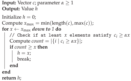
The -operator and - index have been implemented and reference them as Algorithms 1 and 2. The -operator computes a thresholded value h for a given vector c and a parameter . It iteratively evaluates the maximum integer x such that at least x elements in c satisfy the condition . This process identifies a critical point where the density of values in c relative to -scaled thresholds is maximized. The algorithm terminates once the condition is met or exhausts the search range, ensuring computational efficiency by limiting the search to . The output h quantifies the structural resilience or dominance of values in c under the specified -weighted constraint, applicable in scenarios requiring threshold-based analysis of data distributions.
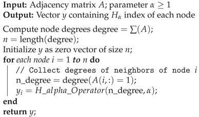
The -index algorithm evaluates the influence of a node in a network by leveraging its neighborhood structure. Given an adjacency matrix A and parameter , it first extracts node degrees degree from A. For each node i, it computes the degrees of its immediate neighbors n_degree and applies the H-alpha operator to this subset. The resulting represents the H-alpha index of node i, reflecting the interplay between the node’s connectivity and the -scaled thresholding of its neighbors’ degrees. This metric provides insights into how local network properties propagate globally, enabling the identification of nodes whose influence is contingent on both their direct connections and the collective behavior of their neighbors.
Classically, the H-sequence converges to its coreness [28]. However, when extended to the -index framework, the iterative sequence converges to zero (See Theorem 1), presenting challenges in generalizing the k-core concept. To address this, we propose accumulating the iterative values during the convergence process, as later termination at zero indicates stronger coreness. This leads to the following definition of g-core, where the summation of values quantifies the structural centrality.
Definition 6.
The g-core of a node v is defined as
Furthermore, to incorporate neighborhood influence, we introduce the local g-core, which integrates the coreness metrics of adjacent nodes, enabling localized structural analysis.
Definition 7.
Local g-core of a node v is defined as
where is a parameter compromising between the node v and its neighbors.
| Algorithm 3:g-core Calculation |
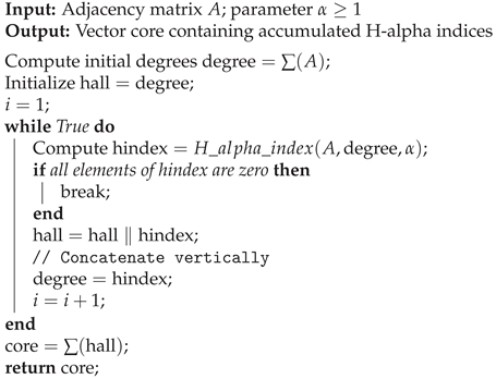 |
The g-core has been implemented in Algorithm 3. The g-core algorithm iteratively refines the structural properties of a network through successive applications of the H-alpha index. Starting with initial node degrees, it computes the H-alpha index vector hindex and updates the degree vector for the next iteration. This process continues until all elements in hindex become zero, signifying that the network’s structural constraints under -scaled thresholds are fully exhausted. The algorithm accumulates intermediate results into a matrix hall, and the final output core is obtained by summing all rows of hall. This cumulative measure captures the network’s progressive degradation under iterative -based filtering, offering a quantitative framework to assess robustness or vulnerability in complex systems.
Table 1 presents the -sequence and g-core values for the nodes in Figure 1. Node in Figure 1 has neighbors with degrees , whereas node has neighbors with degrees . Despite node being structurally more influential than node , their H-indices are equal. This highlights a limitation of the H-index and traditional coreness metrics: they fail to distinguish the true influence of nodes based on neighborhood diversity. In contrast, the g-core and -index values of are strictly greater than those of , demonstrating their capacity to more effectively capture the structural significance of nodes with heterogeneous neighborhood properties.

Table 1.
The H-index, coreness, -sequence and g-core, where .
| Node | ||||||||
|---|---|---|---|---|---|---|---|---|
| 2 | 4 | 3 | 4 | 3 | 2 | 2 | 2 | |
| 2 | 2 | 2 | 2 | 2 | 1 | 1 | 1 | |
| 1 | 1 | 1 | 1 | 1 | 0 | 0 | 0 | |
| 0 | 0 | 0 | 0 | 0 | 0 | 0 | 0 | |
| g-core | 5 | 7 | 6 | 7 | 6 | 3 | 3 | 3 |
| H-index | 2 | 3 | 3 | 3 | 3 | 2 | 2 | 2 |
| coreness | 2 | 3 | 3 | 3 | 3 | 2 | 2 | 2 |
4. Experimental Results
We compare the proposed centralities with degree, H-index, coreness, closeness, betweenness, and CI using Kendall’s tau coefficient and imprecision value on 15 real networks.
4.1. Data Sets
The experiments utilize 15 benchmark networks spanning diverse domains: (1) C.elegansneural network [7]: A neural network of the nematode Caenorhabditis elegans. (2) Email communication network [37]: An email network among university members. (3) Kohonen self-organizing maps [38]: A network representing academic articles on self-organizing maps and related references. (4) Router-level internet topology [39]: A network modeling global internet router connections. (5) Yeast protein interactions [8]: A protein-protein interaction network in budding yeast. (6) US air transportation system [38]: A network representing commercial airline routes in the United States. (7) Scientometrics literature network [38]: A citation network from Scientometrics journal articles (1978-2000). (8) Small-Griffith citation network [38]: A network of citations to works by Small, Griffith, and their descendants. (9) Sexual activity network [40]: A social network derived from a web-based sexual contact community. (10) Condensed matter collaboration network [41]: A collaboration network of scientists sharing preprints in condensed matter physics (1995-2003). (11)Enron email corpus [42]: A large-scale email communication network containing 0.5 million emails. (12) Secure information exchange network [38]: A network of secure information exchange via routers. (13)Arxiv condensed matter collaboration [41]: A network of collaborations among condensed matter physicists. (14)Enron email network [42]: A network derived from 30,000+ emails in the Enron scandal. (15) General network repository [38]: A heterogeneous collection of citation networks. For more detail, see Table 2.
4.2. Evaluation Metrics
4.2.1. SIR Model
We utilize the standard susceptible-infected-recovered (SIR) model [43,44] to evaluate the accuracy of the proposed centralities in identifying vital nodes. In this model, each node transitions through three states: susceptible (S), infected (I), and recovered (R). The spreading influence of a node is defined as the average number of recovered nodes when it serves as the infected source in the SIR process.
The simulation proceeds as follows:
(1) One node is selected as the infected seed, with all others initially susceptible.
(2) At each simulation step, infected nodes transmit the infection to susceptible neighbors with probability , and then transition to the recovered state with probability .
(3) The process terminates when no infected nodes remain.
The total number of recovered nodes at termination quantifies the seed node’s influence. The SIR model’s approximate epidemic threshold [45] is given by:
where denotes the average node degree. Simulations are conducted at , , and , with fixed. Each result represents the average over 100 independent simulations.
4.2.2. Kendall’s Tau Coefficient
As a rank correlation metric [46], Kendall’s tau () quantifies the agreement between node rankings derived from a given centrality and the ground truth (empirical SIR influence). A higher value indicates stronger correlation between the centrality ranking and the actual spreading influence.
4.2.3. Imprecision Value
This metric [47] evaluates a centrality’s ability to identify the most influential nodes. Given a network with n nodes and a fraction :
: cumulative influence of the top nodes ranked by a centrality.
: maximum cumulative influence achievable from any nodes.
The imprecision value is defined as:
Smaller values indicate better performance in prioritizing high-influence nodes.
4.3. Results of Kendall’s Tau Coefficients
Since the local g-core involves two parameters, and , we conduct extensive experiments to analyze their performance across different value combinations. Specifically, we test nine values of and nine values of . Among all combinations, the proposed local g-core achieves the highest performance in terms of Kendall’s tau coefficients when and under the SIR simulation with infected probability . A comprehensive summary of these results is presented in Table 3.
As shown in Table 3, the local g-core outperforms existing centrality measures across all fifteen real-world networks in terms of Kendall’s tau coefficients. Notably, on the networks NS, PGP, and Router, the Kendall’s tau coefficients of local g-core are 45-105% higher than those of classical coreness.
Table 3 also demonstrates that -index slightly better than the classical H-index in terms of Kendall’s tau coefficients. This suggests that considering weak nodes is useful in finding vital nodes. Kendall’s tau coefficients of nine centralities when the infected probability are presented in Table A1 and Table A2 in Appendix A.
4.4. Results of Imprecision Value
The imprecision value focuses exclusively on the most critical nodes in a network. In all experiments, we analyze the top 10% most influential nodes, corresponding to in the imprecision value. The parameters and for the local g-core are identical to those used in Section 3.3. Among all - combinations, the proposed centralities demonstrate strong performance when , , and the infection probability in the SIR simulation is set to . These results are summarized in Table 4.
As shown in Table 4, the local g-core outperforms the remaining centralities across ten real-world networks, while the g-core achieves the best performance on four networks. The imprecision values for nine centralities under infection probabilities and are detailed in Table A3–Table A4 of the Appendix.
4.5. Parameters of Local g-Core
This subsection investigates how the parameters and in the local g-core influence Kendall’s tau coefficients. For brevity, we omit analysis of imprecision values, as their trends are highly consistent with the results presented here.
Figure 2 shows the Kendall’s tau coefficients of the local g-core when , , and . As illustrated, the coefficients achieve their maximum at across nearly all networks. Similar patterns are observed for and under identical and values.
Figure 3 presents the Kendall’s tau coefficients under , , and . The data reveal that the maximum coefficient occurs at on almost all networks. Consistency in performance is maintained across and .
To evaluate the combined impact of and , Figure 4 displays the Kendall’s tau coefficients for the Celegans network across all - combinations. The results confirm that and consistently yield optimal performance for , , and .
5. Conclusions
This paper addresses the challenge of identifying vital nodes in complex networks, where most existing centrality measures inadequately account for weak nodes. To address this limitation, we propose a novel -index, defined as the maximum number of neighbors whose degrees exceed times the degree of the focal node. By iteratively applying the -index to a node’s neighbors, we derive two novel centrality measures: the g-core and local g-core. Experimental results demonstrate that these centralities outperform existing methods in real-world networks, offering a robust framework for node prioritization.
Future research will extend this framework to weighted networks. While the theoretical properties of the -index and g-core in weighted networks align closely with those in unweighted networks, nuanced differences in their behavior and computational dynamics warrant further investigation. This extension will enhance the applicability of our approach to a broader class of networked systems.
Funding
This research received no external funding.
Data Availability Statement
Data sharing not applicable to this article as no datasets were generated or analysed during the current study.
Acknowledgments
The author would like to express his gratitude to the editor and the anonymous reviewers. Their insightful and constructive comments greatly improved the quality and presentation of this paper.
Conflicts of Interest
The author has no relevant financial or non-financial interests to disclose.
Appendix A
Table A1.
Kendall’s tau coefficients comparing nine centralities. For each network, the infection probability is set as , with parameters and . The maximum value in each row is highlighted in boldface to indicate the best performance. Abbreviations: CN (coreness), CC (closeness), BT (betweenness), CI (collective influence), -index (), GC (g-core), and LGC (local g-core).
| Networks | Degree | H-index | CN | CC | BT | CI | GC | LGC | |
|---|---|---|---|---|---|---|---|---|---|
| Celegans | 0.69 | 0.73 | 0.71 | 0.63 | 0.54 | 0.74 | 0.74 | 0.74 | 0.77 |
| 0.81 | 0.85 | 0.84 | 0.81 | 0.64 | 0.87 | 0.86 | 0.89 | 0.91 | |
| Kohonen | 0.65 | 0.66 | 0.67 | 0.71 | 0.52 | 0.69 | 0.67 | 0.67 | 0.77 |
| Metabolic | 0.56 | 0.59 | 0.61 | 0.58 | 0.40 | 0.64 | 0.59 | 0.60 | 0.67 |
| Moreno | 0.62 | 0.63 | 0.64 | 0.74 | 0.52 | 0.75 | 0.66 | 0.70 | 0.75 |
| NS | 0.50 | 0.51 | 0.47 | 0.37 | 0.33 | 0.70 | 0.54 | 0.66 | 0.70 |
| PGP | 0.51 | 0.51 | 0.51 | 0.59 | 0.34 | 0.60 | 0.52 | 0.71 | 0.72 |
| Router | 0.32 | 0.28 | 0.29 | 0.60 | 0.32 | 0.37 | 0.30 | 0.64 | 0.65 |
| SciMet | 0.77 | 0.80 | 0.81 | 0.81 | 0.62 | 0.81 | 0.81 | 0.83 | 0.85 |
| SmaGr | 0.63 | 0.65 | 0.66 | 0.66 | 0.55 | 0.69 | 0.66 | 0.67 | 0.73 |
| USAir | 0.70 | 0.73 | 0.73 | 0.76 | 0.53 | 0.74 | 0.75 | 0.77 | 0.81 |
| Yeast | 0.69 | 0.71 | 0.70 | 0.61 | 0.39 | 0.77 | 0.71 | 0.74 | 0.76 |
| Sex | 0.48 | 0.52 | 0.53 | 0.72 | 0.42 | 0.56 | 0.54 | 0.62 | 0.70 |
| Condmat | 0.56 | 0.61 | 0.61 | 0.72 | 0.33 | 0.74 | 0.63 | 0.76 | 0.76 |
| EmailEnron | 0.49 | 0.49 | 0.49 | 0.49 | 0.43 | 0.53 | 0.51 | 0.51 | 0.53 |
Table A2.
Kendall’s tau coefficients comparing nine centralities. For each network, the infection probability is set as , with parameters and . The maximum value in each row is highlighted in boldface to indicate the best performance. Abbreviations: CN (coreness), CC (closeness), BT (betweenness), CI (collective influence), -index (), GC (g-core), and LGC (local g-core).
| Networks | Degree | H-index | CN | CC | BT | CI | GC | LGC | |
|---|---|---|---|---|---|---|---|---|---|
| Celegans | 0.78 | 0.82 | 0.79 | 0.61 | 0.61 | 0.81 | 0.82 | 0.83 | 0.84 |
| 0.86 | 0.89 | 0.87 | 0.79 | 0.67 | 0.90 | 0.90 | 0.93 | 0.95 | |
| Kohonen | 0.64 | 0.66 | 0.66 | 0.74 | 0.51 | 0.69 | 0.66 | 0.67 | 0.79 |
| Metabolic | 0.60 | 0.63 | 0.65 | 0.56 | 0.43 | 0.67 | 0.64 | 0.67 | 0.73 |
| Moreno | 0.65 | 0.68 | 0.68 | 0.76 | 0.53 | 0.80 | 0.71 | 0.76 | 0.81 |
| NS | 0.46 | 0.47 | 0.44 | 0.39 | 0.30 | 0.66 | 0.52 | 0.63 | 0.66 |
| PGP | 0.46 | 0.48 | 0.48 | 0.65 | 0.32 | 0.57 | 0.50 | 0.73 | 0.75 |
| Router | 0.31 | 0.28 | 0.29 | 0.63 | 0.30 | 0.36 | 0.30 | 0.64 | 0.65 |
| SciMet | 0.81 | 0.85 | 0.85 | 0.80 | 0.64 | 0.84 | 0.85 | 0.88 | 0.89 |
| SmaGr | 0.68 | 0.71 | 0.71 | 0.66 | 0.57 | 0.74 | 0.71 | 0.72 | 0.78 |
| USAir | 0.74 | 0.77 | 0.77 | 0.75 | 0.56 | 0.79 | 0.78 | 0.81 | 0.85 |
| Yeast | 0.66 | 0.69 | 0.68 | 0.64 | 0.37 | 0.76 | 0.69 | 0.77 | 0.77 |
| Sex | 0.48 | 0.52 | 0.54 | 0.75 | 0.41 | 0.56 | 0.56 | 0.66 | 0.74 |
| Condmat | 0.60 | 0.65 | 0.64 | 0.74 | 0.35 | 0.78 | 0.67 | 0.81 | 0.81 |
| EmailEnron | 0.49 | 0.50 | 0.50 | 0.56 | 0.43 | 0.56 | 0.52 | 0.55 | 0.59 |
Table A3.
Imprecision values comparing nine centralities. For each network, the infection probability is set as , with parameters and . The maximum value in each row is highlighted in boldface to indicate the best performance. Abbreviations: CN (coreness), CC (closeness), BT (betweenness), CI (collective influence), -index (), GC (g-core), and LGC (local g-core).
| Networks | Degree | H-index | CN | CC | BT | CI | GC | LGC | |
|---|---|---|---|---|---|---|---|---|---|
| Celegans | 0.0278 | 0.0259 | 0.29 | 0.0784 | 0.0669 | 0.0278 | 0.0309 | 0.0221 | 0.0187 |
| 0.0202 | 0.0086 | 0.0581 | 0.0476 | 0.1 | 0.0138 | 0.0139 | 0.0052 | 0.0038 | |
| Kohonen | 0.1338 | 0.1221 | 0.131 | 0.1249 | 0.202 | 0.0919 | 0.1215 | 0.12 | 0.0789 |
| Metabolic | 0.0623 | 0.0305 | 0.0294 | 0.0378 | 0.172 | 0.0472 | 0.043 | 0.0321 | 0.0294 |
| Moreno | 0.0561 | 0.0344 | 0.0299 | 0.0336 | 0.1977 | 0.0336 | 0.0364 | 0.029 | 0.0223 |
| NS | 0.2135 | 0.2371 | 0.2831 | 0.3389 | 0.2983 | 0.0964 | 0.1953 | 0.1707 | 0.1189 |
| PGP | 0.1257 | 0.0968 | 0.1074 | 0.1316 | 0.5708 | 0.0359 | 0.0905 | 0.034 | 0.035 |
| Router | 0.1934 | 0.1939 | 0.1963 | 0.1262 | 0.2125 | 0.1194 | 0.1922 | 0.1303 | 0.0921 |
| SciMet | 0.0707 | 0.0351 | 0.0446 | 0.1093 | 0.1871 | 0.0453 | 0.0347 | 0.0304 | 0.0262 |
| SmaGr | 0.075 | 0.0529 | 0.0694 | 0.088 | 0.1058 | 0.05 | 0.0685 | 0.0468 | 0.0343 |
| USAir | 0.0111 | 0.0155 | 0.0216 | 0.0359 | 0.2136 | 0.0111 | 0.0155 | 0.007 | 0.007 |
| Yeast | 0.0954 | 0.0779 | 0.0714 | 0.4438 | 0.7509 | 0.0466 | 0.0768 | 0.0099 | 0.0194 |
| Sex | 0.2244 | 0.1582 | 0.1225 | 0.0481 | 0.3132 | 0.0978 | 0.1528 | 0.0898 | 0.072 |
| Condmat | 0.1634 | 0.082 | 0.1127 | 0.1019 | 0.4202 | 0.0515 | 0.0766 | 0.0192 | 0.0287 |
| EmailEnron | 0.0938 | 0.0733 | 0.0684 | 0.065 | 0.2466 | 0.0626 | 0.072 | 0.0677 | 0.0576 |
Table A4.
Imprecision values comparing nine centralities. For each network, the infection probability is set as , with parameters and . The maximum value in each row is highlighted in boldface to indicate the best performance. Abbreviations: CN (coreness), CC (closeness), BT (betweenness), CI (collective influence), -index (), GC (g-core), and LGC (local g-core).
| Networks | Degree | H-index | CN | CC | BT | CI | GC | LGC | |
|---|---|---|---|---|---|---|---|---|---|
| Celegans | 0.0214 | 0.0153 | 0.2181 | 0.0585 | 0.0494 | 0.0214 | 0.0098 | 0.0128 | 0.0093 |
| 0.0101 | 0.006 | 0.0422 | 0.0333 | 0.0634 | 0.0089 | 0.0103 | 0.0028 | 0.0009 | |
| Kohonen | 0.1584 | 0.1333 | 0.1483 | 0.1291 | 0.2332 | 0.0961 | 0.1335 | 0.1281 | 0.0736 |
| Metabolic | 0.0464 | 0.0272 | 0.035 | 0.038 | 0.2058 | 0.0306 | 0.0181 | 0.0239 | 0.0248 |
| Moreno | 0.0369 | 0.0187 | 0.0182 | 0.0377 | 0.1759 | 0.025 | 0.0181 | 0.0136 | 0.0127 |
| NS | 0.1961 | 0.2743 | 0.3073 | 0.2905 | 0.2723 | 0.1025 | 0.232 | 0.198 | 0.1514 |
| PGP | 0.1303 | 0.0957 | 0.1124 | 0.1714 | 0.5518 | 0.0397 | 0.0903 | 0.0321 | 0.0334 |
| Router | 0.1748 | 0.1807 | 0.1797 | 0.129 | 0.2114 | 0.1025 | 0.1758 | 0.1111 | 0.0761 |
| SciMet | 0.0411 | 0.0146 | 0.0335 | 0.0956 | 0.1397 | 0.0311 | 0.0173 | 0.0145 | 0.011 |
| SmaGr | 0.0461 | 0.0306 | 0.0535 | 0.0995 | 0.1164 | 0.0387 | 0.0371 | 0.0238 | 0.0206 |
| USAir | 0.0099 | 0.0131 | 0.0197 | 0.0365 | 0.2044 | 0.0099 | 0.0131 | 0.0053 | 0.0053 |
| Yeast | 0.1072 | 0.0894 | 0.0845 | 0.4123 | 0.7032 | 0.0582 | 0.0856 | 0.0083 | 0.0209 |
| Sex | 0.1842 | 0.1185 | 0.0861 | 0.0583 | 0.2876 | 0.0666 | 0.1132 | 0.054 | 0.0439 |
| Condmat | 0.1107 | 0.0444 | 0.0969 | 0.0881 | 0.3422 | 0.0337 | 0.0393 | 0.0122 | 0.0138 |
| EmailEnron | 0.0611 | 0.0373 | 0.0326 | 0.0453 | 0.2458 | 0.0306 | 0.0363 | 0.0315 | 0.0236 |
References
- Chen, D.; Lü, L.; Shang, M.S.; Zhang, Y.C.; Zhou, T. Identifying influential nodes in complex networks. Physica A: Statistical Mechanics and its Applications 2012, 391, 1777–1787. [Google Scholar] [CrossRef]
- Narayanam, R.; Narahari, Y. A shapley value-based approach to discover influential nodes in social networks. IEEE Transactions on Automation Science and Engineering 2011, 8, 130–147. [Google Scholar] [CrossRef]
- Lü, L.; Chen, D.; Ren, X.L.; Zhang, Q.M.; Zhang, Y.C.; Zhou, T. Vital nodes identification in complex networks. Physics Reports 2016, 650, 1–63. [Google Scholar] [CrossRef]
- Dong, Z.; Chen, Y.; Tricco, T.S.; Li, C.; Hu, T. Hunting for vital nodes in complex networks using local information. Scientific Reports 2021, 11, 9190. [Google Scholar] [CrossRef]
- Fan, T.; Lü, L.; Shi, D.; Zhou, T. Characterizing cycle structure in complex networks. Communications Physics 2021, 4, 272. [Google Scholar] [CrossRef]
- Zhao, Y.; Yang, B. Vital nodes identification method integrating degree centrality and cycle ratio. Chinese Physics B 2025, 34, 038901. [Google Scholar] [CrossRef]
- Watts, D.J.; Strogatz, S.H. Collective dynamics of ’small-world’ networks. Nature 1998, 393, 440–442. [Google Scholar] [CrossRef]
- Von Mering, C.; Krause, R.; Snel, B.; Cornell, M.; Oliver, S.G.; Fields, S.; Bork, P. Comparative assessment of large-scale data sets of protein-protein interactions. Nature 2002, 417, 399–403. [Google Scholar] [CrossRef]
- Strogatz, S.H. Exploring complex networks. Nature 2001, 410, 268–276. [Google Scholar] [CrossRef]
- Hirsch, J.E. An index to quantify an individual’s scientific research output. Proceedings of the National Academy of Sciences 2005, 102, 16569–16572. [Google Scholar] [CrossRef]
- Huang, M.H. Exploring the h-ndex at the institutional level. Online Information Review 2012, 36, 534–547. [Google Scholar] [CrossRef]
- Papić, A. Informetrics: The development, conditions and perspectives. In Proceedings of the 2017 40th International Convention on Information and Communication Technology, Electronics and Microelectronics (MIPRO), May 2017; pp. 700–704. [Google Scholar] [CrossRef]
- Zeng, A.; Shen, Z.; Zhou, J.; Wu, J.; Fan, Y.; Wang, Y.; Stanley, H.E. The science of science: From the perspective of complex systems. Physics Reports 2017, 714-715, 1–73. [Google Scholar] [CrossRef]
- Batista, P.D.; Campiteli, M.G.; Kinouchi, O. Is it possible to compare researchers with different scientific interests? Scientometrics 2006, 68, 179–189. [Google Scholar] [CrossRef]
- von Bohlen und Halbach, O. How to judge a book by its cover? How useful are bibliometric indices for the evaluation of “scientific quality” or “scientific productivity”? Annals of Anatomy - Anatomischer Anzeiger 2011, 193, 191–196. [Google Scholar] [CrossRef] [PubMed]
- Kaur, J.; Radicchi, F.; Menczer, F. Universality of scholarly impact metrics. Journal of Informetrics 2013, 7, 924–932. [Google Scholar] [CrossRef]
- Egghe, L. Theory and practise of the g-index. Scientometrics 2006, 69, 131–152. [Google Scholar] [CrossRef]
- Dorogovtsev, S.N.; Mendes, J.F.F. Ranking scientists. Nature Physics 2015, 11, 882–883. [Google Scholar] [CrossRef]
- Tscharntke, T.; Hochberg, M.E.; Rand, T.A.; Resh, V.H.; Krauss, J. Author Sequence and Credit for Contributions in Multiauthored Publications. PLOS Biology 2007, 5, 1–2. [Google Scholar] [CrossRef]
- Gągolewski, M.; Grzegorzewski, P. A geometric approach to the construction of scientific impact indices. Scientometrics 2009, 81, 617. [Google Scholar] [CrossRef]
- Bornmann, L.; Mutz, R.; Daniel, H.D. The h index research output measurement: Two approaches to enhance its accuracy. Journal of Informetrics 2010, 4, 407–414. [Google Scholar] [CrossRef]
- Bras-Amorós, M.; Domingo-Ferrer, J.; Torra, V. A bibliometric index based on the collaboration distance between cited and citing authors. Journal of Informetrics 2011, 5, 248–264. [Google Scholar] [CrossRef]
- Dodson, M. Citation analysis: Maintenance of h-index and use of e-index. Biochemical and Biophysical Research Communications 2009, 387, 625–626. [Google Scholar] [CrossRef] [PubMed]
- Rochim, A.F.; Muis, A.; Sari, R.F. Improving Fairness of H-index: RA-index. DESIDOC Journal of Library and Information Technology 2018, 38, 378. [Google Scholar] [CrossRef]
- Acuna, D.E.; Allesina, S.; Kording, K.P. Predicting scientific success. Nature 2012, 489, 201–202. [Google Scholar] [CrossRef] [PubMed]
- Penner, O.; Pan, R.K.; Petersen, A.M.; Kaski, K.; Fortunato, S. On the Predictability of Future Impact in Science. Scientific Reports 2013, 3, 3052. [Google Scholar] [CrossRef]
- Schreiber, M. Restricting the h-index to a publication and citation time window: A case study of a timed Hirsch index. Journal of Informetrics 2015, 9, 150–155. [Google Scholar] [CrossRef]
- Lü, L.; Zhou, T.; Zhang, Q.M.; Stanley, H.E. The H-index of a network node and its relation to degree and coreness. Nature Communications 2016, 7. [Google Scholar] [CrossRef]
- Zhai, L.; Yan, X.; Zhang, G. The bi-directional h-index and B-core decomposition in directed networks. Physica A: Statistical Mechanics and its Applications 2019, 531. [Google Scholar] [CrossRef]
- Wu, X.; Wei, W.; Tang, L.; Lu, J.; Lu, J. Coreness and h-Index for Weighted Networks. IEEE Transactions on Circuits and Systems I: Regular Papers 2019, 66, 3113–3122. [Google Scholar] [CrossRef]
- Zeng, A.; Zhang, C.J. Ranking spreaders by decomposing complex networks. Physics Letters, Section A: General, Atomic and Solid State Physics 2013, 377, 1031–1035. [Google Scholar] [CrossRef]
- Liu, J.G.; Ren, Z.M.; Guo, Q. Ranking the spreading influence in complex networks. Physica A: Statistical Mechanics and its Applications 2013, 392, 4154–4159. [Google Scholar] [CrossRef]
- Hu, Q.C.; Yin, Y.S.; Ma, P.F.; Gao, Y.; Zhang, Y.; Xing, C.X. A new approach to identify influential spreaders in complex networks. Wuli Xuebao/Acta Physica Sinica 2013, 62. [Google Scholar] [CrossRef]
- Liu, Y.; Tang, M.; Zhou, T.; Do, Y. Improving the accuracy of the k-shell method by removing redundant links: From a perspective of spreading dynamics. Scientific Reports 2015, 5. [Google Scholar] [CrossRef] [PubMed]
- Wu, J.; Qi, X.; Cao, Z. H-sequences and 2-step coreness in graphs. Discrete Applied Mathematics 2024, 343, 258–268. [Google Scholar] [CrossRef]
- Morone, F.; Makse, H.A. Influence maximization in complex networks through optimal percolation. Nature 2015, 524, 65–68. [Google Scholar] [CrossRef]
- Guimera, R.; Danon, L.; Diaz-Guilera, A.; Giralt, F.; Arenas, A. Self-similar community structure in a network of human interactions. Phys. Rev. E 2003, 68, 065103. [Google Scholar] [CrossRef]
- Batagelj, V.; Mrvar, A. Pajek - Analysis and Visualization of Large Networks. In Proceedings of the Graph Drawing, 9th International Symposium, GD 2001 Vienna, Austria, 2001, Revised Papers, 2001, September 23-26; pp. 477–478. [CrossRef]
- Spring, N.; Mahajan, R.; Wetherall, D.; Anderson, T. Measuring ISP Topologies With Rocketfuel. IEEE/ACM Transactions on Networking 2004, 12, 2–16. [Google Scholar] [CrossRef]
- Rocha, L.E.C.; Liljeros, F.; Holme, P. Simulated epidemics in an empirical spatiotemporal network of 50,185 sexual contacts. PLoS Computational Biology 2011, 7. [Google Scholar] [CrossRef]
- Leskovec, J.; Kleinberg, J.; Faloutsos, C. Graph evolution: Densification and shrinking diameters. ACM Transactions on Knowledge Discovery from Data 2007, 1. [Google Scholar] [CrossRef]
- Leskovec, J.; Lang, K.J.; Dasgupta, A.; Mahoney, M.W. Community structure in large networks: Natural cluster sizes and the absence of large well-defined clusters. Internet Mathematics 2009, 6, 29–123. [Google Scholar] [CrossRef]
- Pastor-Satorras, R.; Castellano, C.; Van Mieghem, P.; Vespignani, A. Epidemic processes in complex networks. Reviews of Modern Physics 2015, 87. [Google Scholar] [CrossRef]
- Moreno, Y.; Pastor-Satorras, R.; Vespignani, A. Epidemic outbreaks in complex heterogeneous networks. European Physical Journal B 2002, 26, 521–529. [Google Scholar] [CrossRef]
- Newman, M.E.J. Spread of epidemic disease on networks. Physical Review E - Statistical, Nonlinear, and Soft Matter Physics 2002, 66, 016128–1. [Google Scholar] [CrossRef] [PubMed]
- Kendall, M.G. A new measure of rank correlation. Biometrika 1938, 30, 81–93. [Google Scholar] [CrossRef]
- Kitsak, M.; Gallos, L.K.; Havlin, S.; Liljeros, F.; Muchnik, L.; Stanley, H.E.; Makse, H.A. Identification of influential spreaders in complex networks. Nature Physics 2010, 6, 888–893. [Google Scholar] [CrossRef]
Figure 1.
Example network illustrating the -index and g-core. The g-core values for nodes and are 5 and 3, respectively.
Figure 1.
Example network illustrating the -index and g-core. The g-core values for nodes and are 5 and 3, respectively.
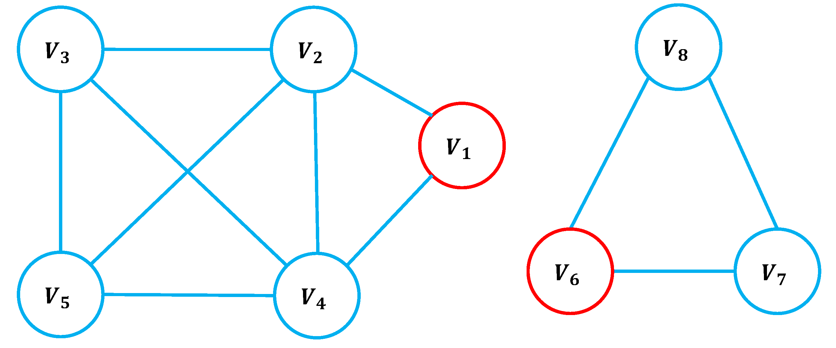
Figure 2.
Kendall’s tau coefficients of local g-core on the fifteen real networks when and . For each network, the infected probability is set as The fifteen networks from left to right are in the same order as the networks in Table 2.
Figure 2.
Kendall’s tau coefficients of local g-core on the fifteen real networks when and . For each network, the infected probability is set as The fifteen networks from left to right are in the same order as the networks in Table 2.
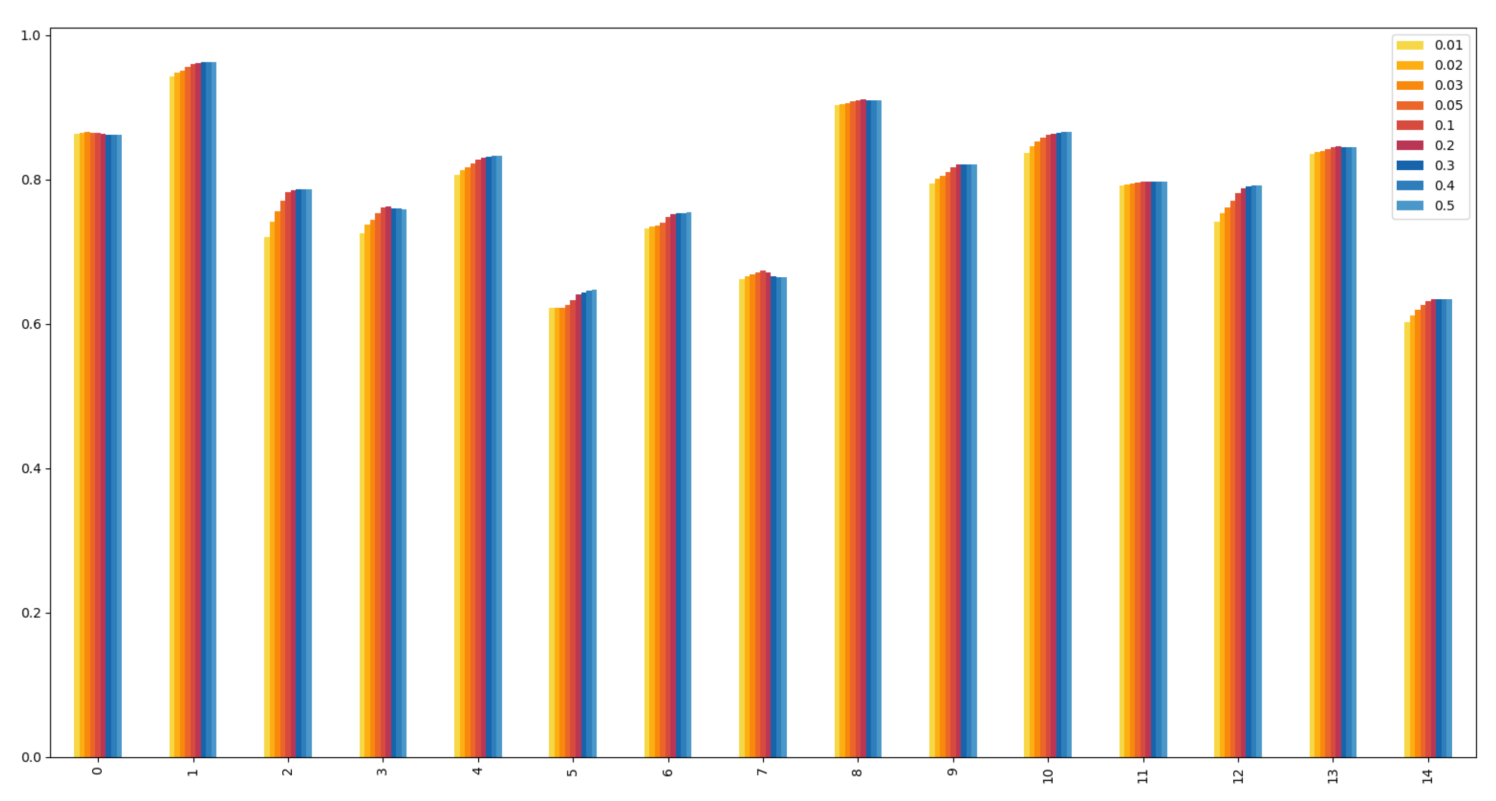
Figure 3.
Kendall’s tau coefficients of local g-core on the fifteen real networks when and . For each network, the infected probability is set as
Figure 3.
Kendall’s tau coefficients of local g-core on the fifteen real networks when and . For each network, the infected probability is set as

Figure 4.
Kendall’s tau coefficients of local g-core on the network Celegns when and . From left to right, the infected probability is set as .
Figure 4.
Kendall’s tau coefficients of local g-core on the network Celegns when and . From left to right, the infected probability is set as .
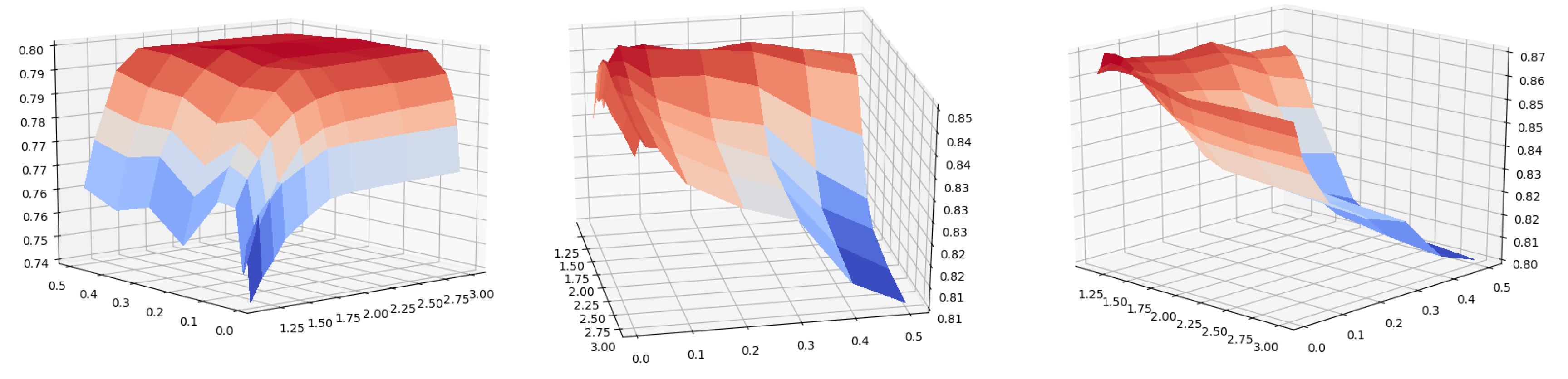
Table 2.
Basic topological features of nine real networks. and denote the number of nodes and the number the links, respectively. <k> and <d> represent the average degree and the average shortest distance, respectively. C is the clustering coefficient, and r is the assortative coefficient.
Table 2.
Basic topological features of nine real networks. and denote the number of nodes and the number the links, respectively. <k> and <d> represent the average degree and the average shortest distance, respectively. C is the clustering coefficient, and r is the assortative coefficient.
| Networks | <k> | <d> | C | r | ||
|---|---|---|---|---|---|---|
| Celegans | 297 | 2148 | 14.46 | 2.46 | 0.308 | -0.163 |
| USAir | 332 | 2126 | 12.81 | 2.74 | 0.749 | -0.208 |
| SmaGr | 379 | 914 | 4.82 | 6.04 | 0.798 | -0.082 |
| Metabolic | 453 | 2025 | 8.94 | 2.66 | 0.646 | -0.226 |
| SciMet | 1059 | 914 | 4.82 | 6.04 | 0.798 | -0.082 |
| 1133 | 5441 | 9.62 | 3.60 | 0.254 | 0.078 | |
| Moreno | 1773 | 9131 | 10.30 | 3.38 | 0.721 | -0.049 |
| NS | 1589 | 2742 | 3.451 | 7.14 | 0.80 | -0.082 |
| Yeast | 2375 | 11693 | 9.85 | 5.09 | 0.388 | 0.454 |
| Kohonen | 4469 | 12718 | 5.69 | 3.67 | 0.211 | -0.121 |
| Router | 5022 | 6258 | 2.49 | 6.45 | 0.033 | -0.138 |
| PGP | 10680 | 24316 | 4.55 | 7.48 | 0.266 | 0.238 |
| Sex | 15810 | 38540 | 4.88 | 5.79 | 0.000 | -0.115 |
| Condmat | 27519 | 116181 | 8.44 | 5.76 | 0.655 | 0.166 |
| EmailEnron | 36692 | 183831 | 10.02 | 3.24 | 0.497 | -0.111 |
Table 3.
Kendall’s tau coefficients comparing nine centralities. For each network, the infection probability is set as , with parameters and . The maximum value in each row is highlighted in boldface to indicate the best performance. Abbreviations: CN (coreness), CC (closeness), BT (betweenness), CI (collective influence), -index (), GC (g-core), and LGC (local g-core).
| Networks | Degree | H-index | CN | CC | BT | CI | GC | LGC | |
|---|---|---|---|---|---|---|---|---|---|
| Celegans | 0.82 | 0.85 | 0.81 | 0.59 | 0.64 | 0.84 | 0.85 | 0.86 | 0.86 |
| 0.88 | 0.91 | 0.88 | 0.78 | 0.68 | 0.91 | 0.91 | 0.93 | 0.96 | |
| Kohonen | 0.64 | 0.66 | 0.67 | 0.73 | 0.51 | 0.69 | 0.67 | 0.68 | 0.79 |
| Metabolic | 0.65 | 0.69 | 0.71 | 0.55 | 0.45 | 0.70 | 0.69 | 0.72 | 0.76 |
| Moreno | 0.68 | 0.71 | 0.71 | 0.76 | 0.55 | 0.81 | 0.74 | 0.80 | 0.83 |
| NS | 0.46 | 0.48 | 0.44 | 0.40 | 0.30 | 0.64 | 0.53 | 0.62 | 0.64 |
| PGP | 0.45 | 0.47 | 0.47 | 0.68 | 0.30 | 0.55 | 0.50 | 0.73 | 0.75 |
| Router | 0.33 | 0.31 | 0.32 | 0.61 | 0.32 | 0.38 | 0.33 | 0.66 | 0.67 |
| SciMet | 0.84 | 0.88 | 0.87 | 0.79 | 0.66 | 0.85 | 0.88 | 0.90 | 0.91 |
| SmaGr | 0.73 | 0.76 | 0.76 | 0.66 | 0.60 | 0.78 | 0.77 | 0.78 | 0.82 |
| USAir | 0.75 | 0.78 | 0.78 | 0.78 | 0.57 | 0.80 | 0.79 | 0.83 | 0.86 |
| Yeast | 0.66 | 0.69 | 0.69 | 0.66 | 0.37 | 0.76 | 0.70 | 0.79 | 0.80 |
| Sex | 0.52 | 0.57 | 0.59 | 0.74 | 0.45 | 0.60 | 0.61 | 0.72 | 0.79 |
| Condmat | 0.63 | 0.68 | 0.67 | 0.73 | 0.37 | 0.79 | 0.71 | 0.84 | 0.85 |
| EmailEnron | 0.49 | 0.50 | 0.50 | 0.60 | 0.43 | 0.58 | 0.53 | 0.58 | 0.63 |
Table 4.
Imprecision values comparing nine centralities. For each network, the infection probability is set as , with parameters and . The maximum value in each row is highlighted in boldface to indicate the best performance. Abbreviations: CN (coreness), CC (closeness), BT (betweenness), CI (collective influence), -index (), GC (g-core), and LGC (local g-core).
| Networks | Degree | H-index | CN | CC | BT | CI | GC | LGC | |
|---|---|---|---|---|---|---|---|---|---|
| Celegans | 0.0103 | 0.0119 | 0.1508 | 0.0470 | 0.0255 | 0.0103 | 0.0161 | 0.0100 | 0.0032 |
| 0.0048 | 0.0050 | 0.0301 | 0.0198 | 0.0393 | 0.0046 | 0.0081 | 0.0023 | 0.0004 | |
| Kohonen | 0.1558 | 0.1376 | 0.1365 | 0.1648 | 0.2603 | 0.1025 | 0.1308 | 0.1204 | 0.0795 |
| Metabolic | 0.0556 | 0.0164 | 0.0268 | 0.0370 | 0.1995 | 0.0338 | 0.0158 | 0.0126 | 0.0187 |
| Moreno | 0.0289 | 0.0112 | 0.0160 | 0.0385 | 0.1748 | 0.0214 | 0.0140 | 0.0094 | 0.0099 |
| NS | 0.1597 | 0.2134 | 0.2477 | 0.2068 | 0.2174 | 0.0955 | 0.2001 | 0.1717 | 0.1404 |
| PGP | 0.1268 | 0.0911 | 0.1157 | 0.1866 | 0.5298 | 0.0427 | 0.0861 | 0.0302 | 0.0316 |
| Router | 0.1385 | 0.1330 | 0.1304 | 0.1379 | 0.1957 | 0.0650 | 0.1255 | 0.0710 | 0.0555 |
| SciMet | 0.0248 | 0.0086 | 0.0310 | 0.0835 | 0.1044 | 0.0210 | 0.0110 | 0.0067 | 0.0059 |
| SmaGr | 0.0330 | 0.0100 | 0.0434 | 0.1020 | 0.0988 | 0.0221 | 0.0220 | 0.0148 | 0.0141 |
| USAir | 0.0062 | 0.0057 | 0.0063 | 0.0218 | 0.1875 | 0.0062 | 0.0057 | 0.0027 | 0.0027 |
| Yeast | 0.0825 | 0.0779 | 0.0858 | 0.3466 | 0.6353 | 0.0448 | 0.0768 | 0.0026 | 0.0090 |
| Sex | 0.1363 | 0.0772 | 0.0494 | 0.0772 | 0.2434 | 0.0428 | 0.0714 | 0.0267 | 0.0243 |
| Condmat | 0.0730 | 0.0254 | 0.0802 | 0.0744 | 0.2735 | 0.0253 | 0.0214 | 0.0142 | 0.0100 |
| EmailEnron | 0.0502 | 0.0254 | 0.0204 | 0.0492 | 0.2551 | 0.0245 | 0.0238 | 0.0196 | 0.0154 |
Disclaimer/Publisher’s Note: The statements, opinions and data contained in all publications are solely those of the individual author(s) and contributor(s) and not of MDPI and/or the editor(s). MDPI and/or the editor(s) disclaim responsibility for any injury to people or property resulting from any ideas, methods, instructions or products referred to in the content. |
© 2025 by the authors. Licensee MDPI, Basel, Switzerland. This article is an open access article distributed under the terms and conditions of the Creative Commons Attribution (CC BY) license (http://creativecommons.org/licenses/by/4.0/).
Copyright: This open access article is published under a Creative Commons CC BY 4.0 license, which permit the free download, distribution, and reuse, provided that the author and preprint are cited in any reuse.


