
Submitted:
10 May 2025
Posted:
12 May 2025
You are already at the latest version
Abstract
For the first time, the problem of determining zonal indicators of electricity production and zonal power values that ensure prospective generation Wx in year x is solved. The developed mathematical model is based on statistical processing of a set of N retrospective daily electrical load graph (ELGi), i is the year index,, each of which has a maximum daily production Wimax in year i. The resulting zonal averages of the generation structure and the annual duration of the maximum power are used to identify from the set of N baseline daily ELGδi one of them that has the best zonal performance in terms of power errors. Such ELGδe is further used as a reference for determining zonal powers Pxb, Pxh and Pxp, as well as their errors. At the same time, the calibration coefficient α is determined by dividing the prospective electricity demand Wx in year x by the annual electricity production Wδe in the retrospective year of the reference ELGδe. It is proved that the zonal capacities Pxb, Pxh, Pxp are equal to the zonal capacities Pδeb, Pδeh and Pδep multiplied by the calibration factor α. It is proved that the errors of Pxb, Pxh, Pxp are identical to the errors of Pδeb, Pδeh and Pδep and therefore are minimal modulo of those possible on the set N of basic ELGδi.
Keywords:
power system
; structure of generating capacities
; electrical load graph
; electricity
; power
; prediction
; accuracy
, each of which has a maximum daily production Wimax in year i. The resulting zonal averages of the generation structure and the annual duration of the maximum power are used to identify from the set of N baseline daily ELGδione of them that has the best zonal performance in terms of power errors. Such ELGδeis further used as a reference for determining zonal powers Pxb, Pxh and Pxp, as well as their errors. At the same time, the calibration coefficient α is determined by dividing the prospective electricity demand Wx in year x by the annual electricity production Wδe in the retrospective year of the reference ELGδe. It is proved that the zonal capacities Pxb, Pxh, Pxp are equal to the zonal capacities Pδeb, Pδeh and Pδep multiplied by the calibration factor α. It is proved that the errors of Pxb, Pxh, Pxp are identical to the errors of Pδeb, Pδeh and Pδep and therefore are minimal modulo of those possible on the set N of basic ELGδi.
1. Introduction
Adequate forecasting of the required volumes of electricity generation and sufficient capacity for integrated power systems (IPS) is crucial given the rapid development of industries and consumption volumes and the growing demands to reduce the harmful impact on the environment by reducing greenhouse gas emissions [1,2,3,4,5,6,7,8,9,10]. As the demand for electricity is also growing due to economic growth, urbanisation and the increasing electrification of industries, reliable long-term forecasting of the required parameters of integrated power systems is becoming important to ensure energy security and grid stability. Integrated power systems, which often connect several regional or national grids, require an integrated approach to accurately forecast demand, supply capabilities and potential problems.
The global trend of rapid deployment of renewable energy sources and the growing focus on reducing carbon emissions are challenging traditional forecasting methods. The successful functioning of the IPS largely depends on balancing electricity availability and peak demand, making accurate long-term forecasting a cornerstone of strategic planning and infrastructure development in the energy sector.
Ensuring the reliable operation of integrated power systems in the context of growing energy consumption, technology development and the integration of renewable energy sources is currently a critical task. Accurate forecasting of the required and sufficient power can be the basis for strategic planning, improving the efficiency of the power system and preventing energy shortages or surpluses.
Models based on regression analysis methods to take into account the dependence of capacities on socio-economic factors (gross domestic product (GDP), population, etc.) are presented in [11,12,13,14,15,16,17,18].
Paper [11] presents a simple model based on regression analysis that includes population and GDP per capita for long-term forecasting of electricity demand. The model, based on energy consumption data for 1990-2012 by sector, generates projected energy demand by sector until 2025.
To predict the future demand for regional energy, [12] analyses the applicable environment and forecasting conditions, performs energy forecasting for Liaoning Province from 2010 to 2019, and compares it with actual data and the elasticity coefficient. The comparison shows that the forecasting accuracy of the proposed model is higher than that of the traditional forecasting method using the elasticity coefficient, which proves the scientificity and effectiveness of the model for regional energy demand forecasting. It is argued that the method and data can provide a reliable database for the planning and development of the future power grid.
The main study [13] is the forecasting of energy demand using Multivariate Adaptive Regression Splines (MARS) as a non-parametric regression technique. Energy demand was modelled for the period 1975-2019 based on a combination of factors, including GDP, population, etc. Five models were created and compared with real data collected by the Ministry of Energy and Natural Resources (MENR). The third model, MARS, was recognised as the best, demonstrating the highest predictive accuracy in forecasting energy demand.
In [14], three years of demand data and its categorical characteristics are divided into four seasons and fed into an efficient regression model called Machine Learning Categorical Boosting (ML CatBoost) to predict demand for the next year. The model uses a new gradient boosting algorithm that works efficiently with categorical features. Five different machine learning models were developed, analysed and tested to predict the hourly total electricity demand using the same data. The proposed model is compared with a long short-term memory neural network and five other ML models using performance evaluation matrices. The importance of accurate forecasting for the integration of clean energy into the grid is discussed.
Traditional demand forecasting models use linear regression, exponential smoothing, pick-up approach and other models for forecasting [15]. These models can be viewed as time series. They have a weak ability to generalise and, ultimately, demonstrate low adaptability to random changes. The proposed support vector regression (SVR) model, which is derived from machine learning, is highly adaptive to nonlinear random data changes and can adaptively account for random disturbances. The model is trained on a vector composed of historical data. Numerical results show that the SVR model significantly improves forecasting accuracy compared to traditional models.
The study [16] aims to apply a first-order model with one variable without using statistical assumptions to forecast energy demand. To improve the accuracy of forecasting, it is necessary to solve the problem arising from the collected samples, which are often based on uncertain estimates. One approach to handling these uncertain and imprecise observations is to use nonlinear interval regression analysis with neural networks to generate upper and lower bounds for individual samples. The study confirmed the high applicability of the proposed model for energy demand forecasting.
The article [17] proposes a two-stage model based on the method of least absolute reduction and selection of variables to determine the factors of energy demand. A support vector regression model with composite data and second-order exponential smoothing (SVR-CDSES) was created to forecast demand for coal, oil, natural gas, and primary electricity. The results of the empirical analysis show that China's energy demand will grow at an annual rate of 2.68% over the next decade. Demand for natural gas and primary electricity will grow rapidly, reaching a maximum annual growth rate of 8.05%, indicating an increased focus on clean energy.
A study [18] created multivariate linear regression models to estimate the expected annual heating energy demand in different building configurations and tested their accuracy. The models were modified in such a way that the complexity increased only to the point where the accuracy of the approximation remained sufficient. The result was a multivariate linear model that estimated the expected outcome for unknown descriptive variables with a relative error of 0% and a standard deviation of 1.6%.
Time series models, such as ARIMA (Auto Regressive Integrated Moving Average) and exponential smoothing [19,20,21,22], use historical data to predict future demand trends based on observed patterns. These models are particularly effective in accounting for seasonal fluctuations and short-term changes in demand.
Study [19] considers the problem of modelling the load of electricity demand. The provided actual load data were deseasonalised and the offline autoregressive moving average model (ARMA) was applied to them using the Akaike's adjusted information criterion (AICC). The obtained results show that the proposed method, based on the theory of multimodel partitioning, successfully solves the task. The developed model can be useful in studies related to forecasting electricity consumption and electricity prices.
Study [20] proposes a vector ETS (VETS) method as a suitable alternative to ARIMA for smoothing and forecasting MF time series. The accuracy of the method's predictions was investigated using Monte Carlo simulations. The results show that the proposed method is suitable for short- and medium-term forecasting.
Study [21] proposes a method for short-term forecasting of the load on the power grid based on an improved exponential smoothing model. Based on a smoothed sequence that corresponds to an exponential trend, a grey forecasting model with an optimised baseline value is created. The inverse exponential smoothing method is used to restore the predicted values. The model takes into account the impact of factors affecting the load on the power grid. The simulation results show that the proposed algorithm has a satisfactory forecasting effect and meets the requirements of short-term load forecasting.
In [22], a multivariate forecasting method of nonlinear exponential smoothing with different weighting factors is investigated to realise short-term power output prediction. The simulations and experimental discussions show that the algorithm proposed in this paper can effectively implement power allocation compared to the traditional one.
New machine learning techniques, such as neural networks and ensemble models, offer improved accuracy by identifying complex patterns in large data sets. These models are becoming increasingly popular due to their adaptability and accuracy in dynamic CPS environments. Examples of the use of machine learning and neural networks for more accurate and adaptive electricity demand estimation are presented in [23,24,25,26,27,28,29,30,31,32].
Scenario-based forecasting takes into account different future conditions, such as policy changes or technological developments, to provide a range of supply and demand projections. This approach is particularly useful when quantitative data is limited. Approaches [33,34,35] are based on scenario modelling to account for the uncertainty of external factors (economic changes, climate impacts).
Reviews of scientific articles devoted to the development and improvement of modelling systems for energy complexes are presented in [36,37,38,39,40].
Even a brief review of the works devoted to the improvement of energy system modelling methods confirms the conclusion about the relevance of updating existing and developing new software and information tools for these purposes. Thus, papers [41,42,43,44,45,46,47,48,49,50,51,52,53,54] describe the most common modern software and information tools aimed at solving these problems.
COHYBEM ‒ Conceptual Hybrid Energy Model for different scales of energy potential [41] is dedicated to bridging the gap between the theoretical foundations of hybrid renewable energy systems and their practical implementation at different scales through the new Conceptual Hybrid Energy Model (COHYBEM). The main goal was to develop a multivariate model that will allow for a new complete and comprehensive technical and economic analysis of the performance of possible hybrid renewable energy systems at different scales. The task is to determine the impact of critical parameters by changing the key variables in the developed model and analysing their consequences. The study includes big data analyses, modelling and optimisation of hybrid energy solutions that combine wind, solar and hydro power with energy storage technology in the form of a pumped storage plant. The study also shows a Pareto curve with increasing installed capacity.
The CYME International T&D software [42] (CYME 9.0 Rev. 4) is, from the authors' point of view, an advanced and comprehensive world-class modelling package developed for transmission, distribution and industrial power systems. The new generation of CYME 9 software supports utilities for modernising the long-term network planning structure. It is built on the basis of such core components as time series analysis, distributed energy resource (DER) optimisation, and no-wire alternatives (NWA). CYME 9.0 aims to integrate the capacity planning process with the distributed resource planning process. It emphasises the power and versatility of the user interface, combining simplicity with efficiency.
Power System Solutions DIgSILENT [43] is a software for analysing power systems: generation, transmission, distribution and industry. It covers a full range of functionality from standard functions to highly complex and advanced applications, including wind energy, distributed generation, real-time modelling and performance monitoring for system testing.
EMMA [44] is an optimisation model for the European integrated power system. It minimises the total system costs, taking into account dispatch and investments in generation, energy storage, and interconnections with hourly granularity. The model includes 14 generation technologies and two energy storage technologies. It takes into account a large number of technical constraints related to short-term system balancing, cogeneration, cyclical operation of thermal power plants, and operational limitations of hydropower facilities. The demand for electricity must be met at every hour of the year, taking into account the cost of under-supply, which is €1,000/MWh. Border crossings are subject to net capacity constraints. However, the model does not include the task of discrete unit commitment and load flow calculations. EMMA is a linear programme with approximately 2 million non-zero elements and is routinely solved using CPLEX, a software package designed to solve linear and quadratic programming problems, including integer programming.
SOPS [45] is a software and information complex of the General Energy Institute of the NAS of Ukraine. The main advantages of the complex are its capabilities:
- ○
- modelling the power system as a complex hierarchical quasi-dynamic system;
- ○
- modelling a multi-node integrated power system with integer variables;
- ○
- minimising the weighted average cost of electricity generation and storage;
- ○
- ong-term technological upgrading of power system components.
The complex allows for optimal selection of power units and their operating modes, ensuring the generation and redistribution of energy in accordance with the consumption schedule. The authors emphasise the versatility of SOPS, which makes it possible to explore various models of power system optimisation in a short time. The user can develop, edit, save and debug optimisation models. The connection of input data, sets, parameters, constants and variables used in the model is organised in a convenient way. You can edit parameters and input data, and then run the model. The modelling results can be displayed on the model worksheets or output as separate files. Another advantage of the software and information complex [45] is the ability to conveniently compare many models, since each of the worksheets can contain its own model.
Enertile [46] is an energy system optimisation model developed at the Fraunhofer Institute for Systems and Innovation Research (Fraunhofer ISI). The model focuses on the electricity sector. Enertile is primarily used for long-term scenario studies and is specifically designed to capture the challenges and opportunities associated with the growing share of renewable energy sources. The main advantage of the model is its high technical and temporal granularity, which allows for a detailed analysis of power systems, taking into account the dynamics of technology development and RES integration.
ENTIGRIS [47] is an electricity market model designed to analyse energy systems from an economic perspective. It takes into account various factors, including market participant configurations and economic indicators, to provide insights into the development of energy systems.
TIMES [48,49] ‒ (acronym for The Integrated MARKAL-EFOM System) is an economic model generator for local, national, multi-regional or global energy systems that provides a technologically rich representation of the dynamics of energy processes over a multi-period time horizon. The model is typically used to analyse the entire energy sector, but can also be used to study specific sectors such as electricity or district heating. TIMES is used to generate energy development scenarios taking into account economic, technological and resource constraints.
TIMES-Ukraine [50] is a linear optimisation model of the energy system that belongs to the MARKAL/TIMES class of models. It provides a multi-technology (bottom-up) representation of the energy system to assess energy dynamics in the long term. The Ukrainian energy system is divided into seven sectors in the model. The structure of the TIMES-Ukraine model follows the methodological approach of the State Statistics Service of Ukraine, which is aligned with the Eurostat and IEA methodology for energy statistics. More than 1.6 thousand technologies are represented in the model.
GENESYS (GENeration Evaluation SYStem) [51] is a model developed to assess the adequacy of energy supply in the Pacific Northwest region under uncertain future conditions. GENESYS is a constrained economic dispatch model that uses the Monte Carlo method to assess the effects of uncertainty. GENESYS is used for: analysing the adequacy of energy supply, modelling the impact of uncertainties in generation and demand.
ARTEMiS [52] is designed for real-time modelling of power systems and power electronics. ARTEMiS provides advanced solvers and algorithms to ensure reliable, accurate computations with fixed time steps, which is essential for real-time simulations. In addition, ARTEMiS uses an advanced decomposition method that does not introduce artificial delays, which is important when modelling large-scale power grids.
LIBEMOD [53] is a multi-country energy equilibrium model based on a set of competitive markets for eight energy commodities: electricity, natural gas, oil, coking coal, lignite, steam coal, biofuels and biomass. All energy commodities are produced and consumed in each of the model countries: EU27, Iceland, Norway and Switzerland.
PowerGAMA [54] optimises generation dispatch, i.e. the power produced by all generators in the power system, based on marginal costs for each time step over a certain period, e.g. one year. It takes into account the variable capacity available for solar, hydro and wind generators, as well as demand variability.
This review allows us to draw the following conclusions:
- ○
- Most models are designed to assess and forecast the economic and technological parameters of the IPS elements and are aimed at solving the problems of minimising current and total operating costs. At the same time, the issues of IPS sustainability and ensuring the required volumes of energy consumption are considered rather as secondary factors that affect the minimisation of these costs and the payback period of investments.
- ○
- Other models focus on the problems of step-by-step (daily, hourly, minute-by-minute, etc.) functioning of the energy system or its elements in the presence of external influences.
Thus, the problem of determining the generalised parameters of the IPS, which determine the required system stability, determined by the values of the projected consumption and, consequently, generation volumes, fades into the background.
The need to develop a comprehensive methodology and mathematical model is becoming an urgent task for the integrated power systems of Ukraine and the world.
2. Methodology for Determining the Necessary and Sufficient Volumes of Capacity in Integrated Power Systems for the Long Term
The task formulated in this study is the first stage of solving a major scientific problem of optimising the prospective power structure of the integrated power system. The purpose of this work is to determine the zonal capacity values that would be able to generate electricity in year x with an annual volume of electricity Wx. After determining these capacities, it will be possible to start calculating the optimal sets of types and capacities of generating sources based on a particular optimisation criterion.
When studying the problems of structural development of the IPS, one of the key ones is that the forecasted prospective volumes of electricity production are developed for the prospective year, while the reported retrospective information on its production is in the form of daily electrical load graphs (ELGs) for the past years. This circumstance radically complicates the problem of determining the necessary zonal capacity volumes of daily ELGs necessary and sufficient to meet the forecast annual demand for electricity.
2.1. Features of Daily ELGs
Daily ELGs have features that can be used to acceptably solve the above problem, both in terms of accuracy and labour intensity.
One of these features is that for each year x with annual electricity production Wx, there is only one daily ELGxmax with maximum daily production. Another feature of such ELGxmax is that its zonal capacities, as well as their sum, are the largest compared to similar indicators of other daily ELGs of the same year. An important feature of the structure of each daily ELG is that its base zone is a clearly and unambiguously formed rectangle, with the width always being the number of hours in a day and the height being the capacity, which ensures the appropriate electricity generation in the base zone under such conditions. In the semi-peak and peak zones of daily ELGs, there is no such clarity, they have an openly irregular shape, but each of them, when solving the necessary tasks, is approximated by a rectangle, whose height is the maximum power value of the corresponding ELG zone, and whose width is the number of hours of the day during which the energy of this ELG zone is generated and the specified power is used (Figure 1).
2.2. Methodology for Determining the Necessary and Sufficient Zonal Capacities Based on the Forecasted Electricity Generation Volumes Wx in Year x
The analysis leads to the conclusion that the solution to the formulated problem will be ensured if, among all daily ELGxof theyear x, a daily ELGxmax is identified, with both zonal and total capacity volumes greater than the corresponding indicators of all other daily ELGs of this year. Indeed, the preceding analysis shows that this event occurs when the daily power generation on a certain (unknown) day is the highest in year x. This is true for both future and retrospective ELGs. As shown below, this is sufficient to develop both a methodology and a mathematical model for the task at hand.
The methodology for determining the necessary and sufficient volumes of zonal capacities that are guaranteed to provide electricity generation in the amount of Wx in year x is as follows.
- On the set N of retrospective data on all daily ELGi,, i is the year index, one ELGimax with maximum electricity production is selected, which becomes the base by i year and ELGδi.
- On the set of N retrospective ELGδi,, the indicators of the structure (weighting factors) of electricity production by zones l= b, h, p (designations for base, half-peak and peak zones, respectively) are determined.
- Using item 2.2 on the set of ELGδi,the indicators are averaged.
- On the set of N daily ELGδi,, the indicators of the daily duration of the maximum power for each of the zones l= b, h, p are determined.
- The daily load peak durations for all zones of daily base ELGδi are converted into annual ones with subsequent zonal averaging, resulting in three zonal averages of annual load peak durations Tbr0, Thr0, Tpr0.
- Using the volumes of electricity production and the indicators of items 2.3 and 2.5, the errors for all ELGδiof the set N are calculated.
- On the set of ELGδi,, one reference ELGδe with the best zonal error performance on the set of ELGδi is selected.
- Calibration of the forecasted production volumes Wx and annual reference production volumes Wδe is carried out with further determination of zonal capacities, zonal volumes of electricity production forecast and relevant accuracy indicators.
3. Mathematical Model for Determining the Prospective Capacities in the IPS Based on the Forecasted Generation Volumes
3.1. Determination of the Reference Daily ELGδi
On the set of N daily ELGδi, three-dimensional vectors of the coefficients of the zonal structure of the required values are determined. In particular, the vector of electricity generation structure for ELGδi has the form:
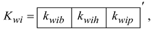 where the zonal coefficients Kwib, Kwih, Kwip are defined as follows:
where Wib, Wih, Wip are the volumes of zonal electricity generation for the i-th daily base ELGsδi, and Wi is their sum.
where the zonal coefficients Kwib, Kwih, Kwip are defined as follows:
where Wib, Wih, Wip are the volumes of zonal electricity generation for the i-th daily base ELGsδi, and Wi is their sum.
On the set of N base of ELGsδi, the average indicators of the coefficients of the zonal structure of the annual electricity production of the base ELGsδi , are determined:
where the index "0" means an averaging operation.
The average annual duration of maximum load usage in zones l= b, h, p of ELGδiis determined as follows:
where Tib, Tih, Tip are the duration of the use of the maximum load of the i-th daily baseline ELGδi in the designated zones, Tr is the number of days in the respective year x
Using the coefficients (5) - (7) and the actual annual electricity production Wi in year i, , zonal indicators are determined according to the following dependencies:
The availability of the calculated indicators (11) - (13) and (8) - (10) makes it possible to determine the zonal capacities of the entire set of basic daily ELGδi, according to the following dependencies:
The basic ELGδicontains data on actual capacity indicators (14) - (15), which makes it possible to determine the methodological error of these dependencies in both absolute and relative terms:
where Δ is the absolute error, ψ is the relative error, l= b, h, p are notations for any zone of the ELG, f is the designation for the actual value.
After determining the indicators (14) - (18) for all the ELGδi, one with the smallest modules of indicators (18) is selected among them, and it is further used as a reference one with the designation ELGδi.
3.2. Determination of the Necessary and Sufficient Zonal Capacity Volumes to Ensure the Forecast Electricity Production Wx in Year x
This task can be most effectively solved by calibrating the reference ELGie using the following algorithm. The calibration coefficient is determined by the formula:
Since the maximum load lifetime for the base zone is a constant, the base zone capacity is automatically determined as:
Because the dependence (19) can be used in the form , the powers Pxh and Pxp are defined as follows:
Using (20) - (22), we determine the zonal indicators of annual electricity production:
Thus, given the forecast value of annual electricity production Wx in year x, the zonal capacities of the daily schedule with maximum electricity production ELGxmax are determined by multiplying the relevant zonal capacity indicators of the reference ELGie by the calibration factor according to (19) - (22). The zonal indicators of annual electricity production in the same year are determined similarly according to (23) - (25).
4. Modelling and Analysis
To apply model (1)-(25), it is sufficient to have only one baseline retrospective ELGδiand one annual forward-looking electricity demand forecast Wx in year x.
The study used redundant arrays of initial retrospective information, namely, four basic ELGsδi and three forecasts Wx, to improve the accuracy of forecasting zonal power and generation indicators (Table 1 and Table 2).
The use of the averaged indicators of the generation structure (5)-(7) and the averaged annual duration of the maximum zonal load (8)-(10) made it possible to simultaneously solve several important tasks: to prove that the sum of zonal generation indicators Ws for each of the ELGδi, with zero error coincides with the actual data of electricity production Wi in year i (Table 3); to prove that the reference ELGδe (2019 year) has zonal generation and capacity errors that do not exceed 0.39% and 1.02% by modulo, respectively; this gives grounds for applying the specified dependencies to determine zonal generation and capacity indicators for the forecast annual generation volumes Wi in years i (Table 3 and Table 4).
However, the issue of errors in zonal indicators of annual electricity generation and zonal capacities for future years remains unresolved. To solve it, the authors developed the calibration method (19)-(25), which generates forecasting errors of zonal generation and capacity at total future annual generation volumes Wx not worse than the errors of the reference ELGδe, namely, |Δ |≤0.39% for generation and |Δ |≤1.02% for capacity (Table 5 and Table 6).
In assessing the level of error of the above indicators, we took into account a criterion that is widely used in feasibility studies. Competing long-term feasibility projects are considered equivalent if the errors in their key indicators do not exceed 5%.
Thus, the calibration method (19) - (25) developed and implemented in this study more than satisfies the above criterion of permissible error.
5. Conclusions
Electricity is a highly valuable commodity with a high degree of technological transformation. Activities in the electricity sector provide high added value. Power generation equipment is high-tech and expensive. The residual life of the equipment of the power system, which is comparable to the Ukrainian one, is estimated to be around USD 80-100 billion. In the context of the post-war restoration of the power system of Ukraine, the required investment will increase at least threefold. Under such conditions, the requirements for the accuracy of the models used to forecast the future structure of the power system's generating capacities will be significantly increased. While in peacetime the permissible error in determining zonal capacities could be up to 5%, in the context of the power system restoration, such an error could result in USD 12-15 billion of additional investments. This would be extremely undesirable in the post-war period.
Therefore, in the course of these studies, a methodology and a mathematical model were developed and synthesised to determine the necessary and sufficient zonal capacities that ensure predetermined volumes of electricity production with an accuracy limited only by the accuracy of the initial information.
Two methods were used to achieve these results within the same model. At the first stage, the least-squares method (averaging) is used to identify the reference ELG from the set of base ELGδi,. The detected ELGiehas the lowest errors in capacity and generation modules compared to other base ELGδi. In this way, the errors of the initial information are filtered (minimised).
At the second stage of calculations using this model, the calibration method is used. This new method virtually identically transfers the indicators from the accuracy of the reference ELGieto the ELGxmax of the daily maximum electricity generation at its annual production Wx in year x. It is the organic combination of these methods within one model that ensures the obtaining of zonal power indicators and, as a result, the generation of the daily ELGxmax with an accuracy limited only by the errors of the initial information of the retrospective daily base ELGδi,. The application of the developed model on the real data of the Ukrainian power system (Table 1 and Table 2) showed that it forms decisions on zonal power Pxl and generation Wxl with high accuracy, namely, the error of zonal power by module does not exceed 1.02% and generation ‒ 0.39% (Table 5 and Table 6).
In the future, to solve the problem of optimising the structure of power system generating capacities for a given period with a given electricity production, it is necessary to use this model to determine the necessary and sufficient zonal capacities, and then to optimise the structure of its generation for each zone using universal software systems.
Author Contributions
Conceptualization, A.Z.; M.K. and V.D.; methodology, A.Z and V.D.; software, V.D.; validation, A.Z.; V.B. and V.D.; formal analysis, M.K and V.B.; investigation, A.Z.; M.K.; V.B. and V.D.; resources, V.D.; data curation, M.K. and V.D.; writing—original draft preparation, A.Z. and V.D.; writing—review and editing, A.Z and V.B.; visualization, A.Z. and M.K.; supervision, M.K.; project administration, A.Z.; funding acquisition, A.Z and V.D. All authors have read and agreed to the published version of the manuscript.
Acknowledgments
This work was supported by the next projects: “Integrated modeling for robust management of food-energy-water-social-environmental (FEWSE) nexus security and sustainable development” (IIASA-NASU, 22-501 (R-45-T)), “Comprehensive analysis of robust preventive and adaptive measures of food, energy, water and social management in the context of systemic risks and consequences of COVID-19” (0122U000552, 2022–2026), and “Development of the structure and ensuring the functioning of self-sufficient distributed generation” (0125U001572, 2025–2026), which are financed by National Academy of Science of Ukraine.
Conflicts of Interest
The authors declare no conflicts of interest.
Abbreviations
The following abbreviations are used in this manuscript:
| ELG | electrical load graph |
| GDP | gross domestic product |
| IPS | integrated power systems |
References
- Hotra, O.; Kulyk, M.; Babak, V.; Kovtun, S.; Zgurovets, O.; Mroczka, J.; Kisala, P. Organisation of the Structure and Functioning of Self-Sufficient Distributed Power Generation. Energies 2024, 17, 27. [Google Scholar] [CrossRef]
- Denysov, V.; Kulyk, M.; Babak, V.; Zaporozhets, A.; Kostenko, G. Modeling Nuclear-Centric Scenarios for Ukraine’s Low-Carbon Energy Transition Using Diffusion and Regression Techniques. Energies 2024, 17, 5229. [Google Scholar] [CrossRef]
- Babak, V.P.; Babak, S.V.; Eremenko, V.S.; Kuts, Y.V.; Myslovych, M.V.; Scherbak, L.M.; Zaporozhets, A.O. (2021). Models of Measuring Signals and Fields. In: Models and Measures in Measurements and Monitoring. Studies in Systems, Decision and Control, vol 360. Springer, Cham. [CrossRef]
- Babak, V.P.; Kulyk, M.M. Possibilities and Perspectives of the Consumers-Regulators Application in Systems of Frequency and Power Automatic Regulation. Tekhnichna Elektrodynamika 2023, 2023, 72–80. [Google Scholar] [CrossRef]
- Nikitin, Y.; Yevtukhova, T.; Novoseltsev, O.; & Komkov, I. (2024). Regional Energy Efficiency Programs. Current Status and Development Prospects. Energy Technologies & Resource Saving 2024, 78, 34–47. [CrossRef]
- Bielokha, H.; Chupryna, L.; Denisyuk, S.; Eutukhova, T.; Novoseltsev, O. (2023). Hybrid energy systems and the logic of their service-dominant implementation: screening the pathway to improve results. Energy Engineering 2023, 120, 1307–1323. [CrossRef]
- Quasi-dynamic Energy Complexes Optimal Use on the Forecasting Horizon / V. Denysov et al. Studies in Systems, Decision and Control. Cham, 2024. P. 81–107. [CrossRef]
- Energy System Optimization Potential with Consideration of Technological Limitations / V. Denysov et al. Studies in Systems, Decision and Control. Cham, 2024. P. 113–126. URL. [CrossRef]
- Zaporozhets, A.; Babak, V.; Kostenko, G.; Zgurovets, O.; Denisov, V.; Nechaieva, T. (2024). Power System Resilience: An Overview of Current Metrics and Assessment Criteria. In: Babak, V.; Zaporozhets, A. (eds) Systems, Decision and Control in Energy VI. Studies in Systems, Decision and Control, vol 561. Springer, Cham. [CrossRef]
- Zaporozhets, A.; Kostenko, G.; Zgurovets, O.; Deriy, V. (2024). Analysis of Global Trends in the Development of Energy Storage Systems and Prospects for Their Implementation in Ukraine. In: Kyrylenko, O.; Denysiuk, S.; Strzelecki, R.; Blinov, I.; Zaitsev, I.; Zaporozhets, A. (eds) Power Systems Research and Operation. Studies in Systems, Decision and Control, vol 512. Springer, Cham. [CrossRef]
- Kumar, J.K.; Ravi, G. A Simple Regression Model for Electrical Energy Forecasting. International Journal of Advanced Research in Electrical, Electronics and Instrumentation Engineering 2014, 3, 11331–11335. [CrossRef]
- Forecast and Analysis of Regional Energy Demand Based on Grey Linear Regression Forecast Model / M. Zhang et al. IOP Conference Series: Earth and Environmental Science 2021, 645, 012047. [CrossRef]
- Prediction of transportation energy demand: Multivariate Adaptive Regression Splines / M. A. Sahraei et al. Energy 2021, 224, 120090. URL. [CrossRef]
- Regression model-based hourly aggregated electricity demand prediction / R. Panigrahi et al. Energy Reports 2022, 8, 16–24. URL. [CrossRef]
- Support vector regression model for flight demand forecasting / W. FAN et al. International Journal of Engineering Business Management 2023, 15, 184797902311743. [CrossRef]
- Integrating Nonlinear Interval Regression Analysis with a Remnant Grey Prediction Model for Energy Demand Forecasting / Y.-C. Hu et al. Applied Artificial Intelligence. [CrossRef]
- Energy demand forecasting in China: A support vector regression-compositional data second exponential smoothing model / C. Rao et al. Energy 2023, 263, 125955. [CrossRef]
- Applicability of Multivariate Linear Regression in Building Energy Demand Estimation / T. Storcz et al. Mathematical Modelling of Engineering Problems 2022, 9, 1451–1458. [CrossRef]
- Electricity demand loads modeling using AutoRegressive Moving Average (ARMA) models / S. S. Pappas et al. Energy 2008, 33, 1353–1360. [CrossRef]
- Seong, B. Smoothing and forecasting mixed-frequency time series with vector exponential smoothing models. Economic Modelling 2020, 91, 463–468. URL. [CrossRef]
- Short-Term Power Load Forecasting Method Based on Improved Exponential Smoothing Grey Model / J. Mi et al. Mathematical Problems in Engineering 2018, 2018, 1–11. [CrossRef]
- Zheng, X.; Jin, T. A reliable method of wind power fluctuation smoothing strategy based on multidimensional non-linear exponential smoothing short-term forecasting. IET Renewable Power Generation 2022. [CrossRef]
- Instantaneous Electricity Peak Load Forecasting Using Optimization and Machine Learning / M. Saglam et al. Energies 2024, 17, 777. [CrossRef]
- Kyi, S.; Taparugssanagorn, A. IoT and machine learning models for multivariate very short-term time series solar power forecasting. IET Wireless Sensor Systems 2024. [CrossRef]
- Benti, N.E.; Chaka, M.D.; Semie, A.G. Forecasting Renewable Energy Generation with Machine Learning and Deep Learning: Current Advances and Future Prospects. Sustainability 2023, 15, 7087. [Google Scholar] [CrossRef]
- A novel machine learning approach for estimation of electricity demand: An empirical evidence from Thailand / E. S. Mostafavi et al. Energy Conversion and Management 2013, 74, 548–555. [CrossRef]
- Improved estimation of electricity demand function by using of artificial neural network, principal component analysis and data envelopment analysis / A. Kheirkhah et al. Computers & Industrial Engineering 2013, 64, 425–441. [CrossRef]
- Solyali, D. A Comparative Analysis of Machine Learning Approaches for Short-/Long-Term Electricity Load Forecasting in Cyprus. Sustainability 2020, 12, 3612. [Google Scholar] [CrossRef]
- Machine and deep learning approaches for forecasting electricity price and energy load assessment on real datasets / H.-A. I. El-Azab et al. Ain Shams Engineering Journal 2024, 102613. [CrossRef]
- Ortiz-Arroyo, D.; Skov, M.K.; Huynh, Q. Accurate Electricity Load Forecasting with Artificial Neural Networks. International Conference on Computational Intelligence for Modelling, Control and Automation and International Conference on Intelligent Agents, Web Technologies and Internet Commerce (CIMCA-IAWTIC'06), Vienna, Austria, 2005, pp. 99. [CrossRef]
- Hu, H.; Gong, S.; Taheri, B. Energy demand forecasting using convolutional neural network and modified war strategy optimization algorithm. Heliyon 2024, e27353. [Google Scholar] [CrossRef]
- Jain, A.; Gupta, S.C. Evaluation of electrical load demand forecasting using various machine learning algorithms. Frontiers in Energy Research 2024, 12, 1408119. [Google Scholar] [CrossRef]
- Mohammed, N.A.; Al-Bazi, A. An adaptive backpropagation algorithm for long-term electricity load forecasting. Neural Comput & Applic 2022, 34, 477–491. [CrossRef]
- Plaga, L.S.; Bertsch, V. Methods for assessing climate uncertainty in energy system models – A systematic literature review. Applied Energy 2023, 331, 120384. [Google Scholar] [CrossRef]
- Pilpola, S.; Lund, P.D. Analyzing the effects of uncertainties on the modelling of low-carbon energy system pathways. Energy 2020, 201, 117652. [Google Scholar] [CrossRef]
- Climate change impacts on the energy system: a model comparison / V. Zapata et al. Environmental Research Letters 2022, 17, 034036. [CrossRef]
- Senatla, M.; Bansal, R.C. Review of planning methodologies used for determination of optimal generation capacity mix: the cases of high shares of PV and wind. IET Renewable Power Generation 2018, 12, 1222–1233. [Google Scholar] [CrossRef]
- Nema, P.; Nema, R.K.; Rangnekar, S. A current and future state of art development of hybrid energy system using wind and PV-solar: A review. Renewable and Sustainable Energy Reviews 2009, 13, 2096–2103. URL. [CrossRef]
- Zhang, T.; et al. Long-Term Energy and Peak Power Demand Forecasting Based on Sequential-XGBoost. IEEE Transactions on Power Systems 2024, 39, 3088–3104. [Google Scholar] [CrossRef]
- Sánchez-Durán, R.; Luque, J.; Barbancho, J. Long-Term Demand Forecasting in a Scenario of Energy Transition. Energies 2019, 12, 3095. [Google Scholar] [CrossRef]
- Conceptual Hybrid Energy Model for Different Power Potential Scales: Technical and Economic Approaches / H. M. Ramos et al. Renewable Energy 2024, 121486. [CrossRef]
- Advanced and comprehensive world-class simulation package CYME 9.0 Rev.4 - Damas Wiki. https://www.damaswiki.net/node/282031.
- DIgSILENT Power Generation. Power System Solutions DIgSILENT. https://www.digsilent.de/en/power-generation.html.
- The Electricity Market Model EMMA. The European Electricity Market Model. https://emma-model.
- Denysov, V.; Babak, V. Software and information simulation complex GEINASU SIC of multi-node integrated and autonomous power and heat supply systems. System Research in Energy 2023, 2023, 50–63. [Google Scholar] [CrossRef]
- The Enertile optimisation model. Enertile® website. https://enertile.eu/enertile-en/methodology/optimisation.php.
- ENTIGRIS an electricity market model for analyzing energy systems from an economic perspective. Wissensplattform - Digitalisierung Energiewendebauen. https://wissen-digital-ewb.de/en/tool_list/businessApps/793.
- Loulou, R.; Labriet, M. ETSAP-TIAM: the TIMES integrated assessment model Part I: Model structure. Computational Management Science 2007, 5, 7–40. [Google Scholar] [CrossRef]
- Loulou, R. ETSAP-TIAM: the TIMES integrated assessment model. part II: mathematical formulation. Computational Management Science 2007, 5, 41–66. [CrossRef]
- TIMES Ukraine. https://www.timesukraine.tokni.com/about.
- GENESYS Model. Northwest Power and Conservation Council. https://www.nwcouncil.org/2021powerplan_genesys-model/.
- ARTEMIS | CPU-BASED ELECTRICAL TOOLBOX. OPAL-RT. https://www.opal-rt.com/solver/.
- LIBEMOD - Frischsenteret. Forside - Frischsenteret. https://www.frisch.uio.no/ressurser/LIBEMOD/About%20the%20model/.
- Svendsen, H. Power Grid and Market Analysis (PowerGAMA). SINTEF. https://www.sintef.no/en/software/power-grid-and-market-analysis-powergama/.
Figure 1.
Typical ELG in the IPS of Ukraine (data for 28.01.2019, day of the 2019 year with the maximum electricity production).
Figure 1.
Typical ELG in the IPS of Ukraine (data for 28.01.2019, day of the 2019 year with the maximum electricity production).
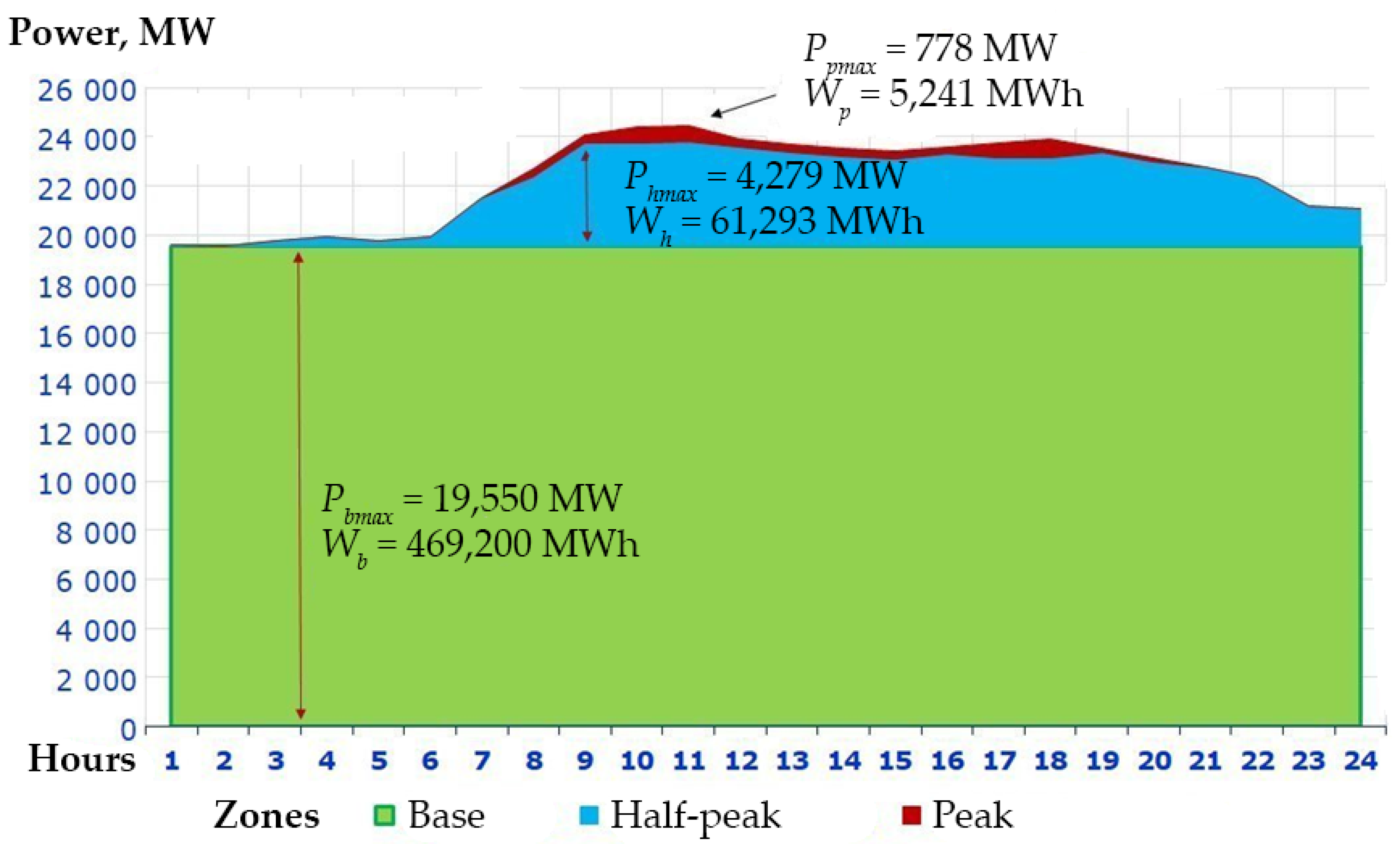

Table 1.
Baseline information: annual zonal electricity production.
| Year | Wf | Wfb | Wfh | Wfp |
| 2016 | 194,338 | 170,348 | 22,293 | 1,696 |
| 2017 | 194,558 | 170,680 | 21,959 | 1,919 |
| 2019 | 195,543 | 171,258 | 22,372 | 1,913 |
| 2020 | 190,749 | 163,672 | 24,847 | 2,230 |
Table 2.
Baseline information: zonal structure of annual electricity production; actual zonal maximum capacity; annual zonal duration of maximum capacity use.
Table 2.
Baseline information: zonal structure of annual electricity production; actual zonal maximum capacity; annual zonal duration of maximum capacity use.
| Structure | Power, MW | Duration, h | |||||||
| Year | Kb | Kh | Kp | Pfb | Pfh | Pfp | Tb | Th | Tp |
| 2016 | 0.8766 | 0.1147 | 0.0087 | 19,393 | 4,959 | 1,022 | 8,784 | 4,483 | 1,655 |
| 2017 | 0.8773 | 0.1129 | 0.0099 | 19,484 | 4,074 | 863 | 8,760 | 5,390 | 2,223 |
| 2019 | 0.8758 | 0.1144 | 0.0098 | 19,550 | 4,279 | 778 | 8,760 | 5,228 | 2,459 |
| 2020 | 0.8580 | 0.1303 | 0.0117 | 18,684 | 4,713 | 1,083 | 8,784 | 5,272 | 2,059 |
| Ave. | 0.8719 | 0.1181 | 0.0100 | 19,278 | 4,506 | 937 | 8,772 | 5,093 | 2,099 |
Table 3.
Predictive annual zonal electricity generation volumes corresponding to the base ELGδi of the given years.
Table 3.
Predictive annual zonal electricity generation volumes corresponding to the base ELGδi of the given years.
| Forecast of annual generation of base ELGδi, 103MWh | |||||
| Year | Wi | Wib | Wih | Wip | Wi-Ws |
| 2016 | 194,338 | 169,447 | 22,944 | 1,947 | 0 |
| 2017 | 194,558 | 169,639 | 22,970 | 1,949 | 0 |
| 2019 | 195,543 | 170,498 | 23,086 | 1,959 | 0 |
| 2020 | 190,749 | 166,318 | 22,520 | 1,911 | 0 |
Table 4.
Forecast of zonal capacities of base ELGδiand determination of zonal errors of capacities and electricity production.
Table 4.
Forecast of zonal capacities of base ELGδiand determination of zonal errors of capacities and electricity production.
| Zonal generation forecast errors, % | Forecast of zonal capacities, MW | Zonal capacity errors, % | |||||||
| Year | ψWb | ψWh | ψWp | Pib | Pih | Pip | ψPb | ψPh | ψPp |
| 2016 | -0.46 | 0.33 | 0.13 | 19317 | 4505 | 927 | -0.31 | -1.84 | -0.38 |
| 2017 | -0.53 | 0.52 | 0.02 | 19339 | 4510 | 928 | -0.59 | 1.76 | 0.26 |
| 2019 | -0.39 | 0.37 | 0.02 | 19437 | 4533 | 933 | -0.46 | 1.02 | 0.62 |
| 2020 | 1.39 | -1.22 | -0.17 | 18960 | 4421 | 910 | 1.14 | -1.20 | -0.71 |
Table 5.
Forecast of prospective annual zonal electricity production (× 103MWh) and zonal capacities (MW) for the selected years by averaging the generation structure.
Table 5.
Forecast of prospective annual zonal electricity production (× 103MWh) and zonal capacities (MW) for the selected years by averaging the generation structure.
| Year | Wx | Wxb | Wxh | Wxp | Wx-Ws | Pxb | Pxh | Pxp |
| 2027 | 171,685 | 149,695 | 20,270 | 1,720 | 0 | 17,065 | 3,980 | 819 |
| 2030 | 215,909 | 188,256 | 25,491 | 2,163 | 0 | 21,461 | 5,005 | 1,030 |
| 2040 | 267,225 | 232,999 | 31,549 | 2,677 | 0 | 26,562 | 6,194 | 1,275 |
Table 6.
Estimation of relative errors in forecasting zonal electricity generation and zonal capacities for selected years by the calibration method.
Table 6.
Estimation of relative errors in forecasting zonal electricity generation and zonal capacities for selected years by the calibration method.
| Year | α | ψWxb, % | ψWxh, % | ψWxp, % | ψPxb, % | ψPxh, % | ψPxp, % |
| 2027 | 0.878 | -0.39 | 0.37 | 0.02 | -0.46 | 1.02 | 0.62 |
| 2030 | 1.104 | -0.39 | 0.37 | 0.02 | -0.46 | 1.02 | 0.62 |
| 2040 | 1.366 | -0.39 | 0.37 | 0.02 | -0.46 | 1.02 | 0.62 |
Disclaimer/Publisher’s Note: The statements, opinions and data contained in all publications are solely those of the individual author(s) and contributor(s) and not of MDPI and/or the editor(s). MDPI and/or the editor(s) disclaim responsibility for any injury to people or property resulting from any ideas, methods, instructions or products referred to in the content. |
© 2025 by the authors. Licensee MDPI, Basel, Switzerland. This article is an open access article distributed under the terms and conditions of the Creative Commons Attribution (CC BY) license (http://creativecommons.org/licenses/by/4.0/).
Copyright: This open access article is published under a Creative Commons CC BY 4.0 license, which permit the free download, distribution, and reuse, provided that the author and preprint are cited in any reuse.


