
Submitted:
21 October 2025
Posted:
22 October 2025
You are already at the latest version
Abstract
This study evaluates the feasibility of fully renewable energy systems on El Hierro, the smallest and most isolated Canary Archipelago Island (Spain), contributing to the broader effort to decarbonize the European economy. By 2040, the island’s energy demand is projected to reach 80–110 GWh annually, assuming full economic decarbonization. Currently, El Hierro faces challenges due to its dependence on fossil fuels and inherent variability of renewable sources, which fluctuate with weather conditions. To ensure system reliability, the study emphasizes the integration of renewable and storage technologies. Two scenarios are modeled using HOMER software with probabilistic methods to capture variability in generation and demand. The first scenario represents the current system enhanced with electric vehicles, while the second incorporates energy efficiency improvements and collective mobility policies to reduce demand. Both prioritize electrification and derive an optimal generation mix based on economic and technical constraints, aiming for the lowest Levelized Cost Of Energy (LCOE). The approach takes advantage of El Hierro’s abundant solar and wind resources, complemented by reversible pumped hydro storage and megabatteries. Results demonstrate that fully renewable systems can reliably meet demand with approximately 30% energy surplus and LCOE near 10 c€/kWh. Uncertainty analysis increases these figures by about 10% both in costs and excesses.
Keywords:
uncertainty analysis
; Best Estimate Plus Uncertainty (BEPU) analysis
; Wilks Formula
; energy balance forecasts
; hybrid renewable energy system
; sustainable energy transition
1. Introduction
1.1. Background on Renewable Energy Systems: The Path to Sustainability
The IEA report "World Energy Outlook 2023" [1] states that global energy demand has uninterruptedly increased over the last few decades, except for the interruption caused by the COVID-19 pandemic in 2020. However, the upward trend resumed in 2021 despite the ongoing pandemic [2]. Historically and up to the present, most of this produced energy comes from fossil fuels, and similar figures are observed in electricity generation. It is true that in recent years, various countries have been investing in the implementation of different renewable energy generation sources. Nevertheless, nearly two-thirds of energy is still generated through fossil fuels [3], although these figures are gradually decreasing year by year [4].
As many experts emphasize, reliance on fossil fuel-based generation is unsustainable and poses two fundamental problems. Firstly, the inevitable depletion of fossil fuels in the medium term if the current consumption rate is maintained [5,6]. The second problem is the pollutant emissions, especially the substantial release of GreenHouse Gases (GHGs) during energy production when fossil fuels are used as fuels or raw materials [7,8].
Therefore, there are many reasons for renewable energies to be present or even to be the only sources of generation used, with the aim of reducing or eliminating fossil fuels and their consequent emissions [9]. Focusing on electricity generation, the use of renewable energies is a necessity, as otherwise, it is impossible to achieve the ambitious GHG emissions reduction targets [10]. Furthermore, the sharp increase in electricity use, which encompasses the final energy consumption of all countries [11], is expected to exceed 30% of the total amount in a short time in many of them [12].
The described problem is further complicated in remote regions, such as islands [13]. This is because their small size and inaccessible location make connecting to a large grid difficult or even technically or economically impossible. Therefore, in the case of islands, the typical solution is to have an energy system based on fossil fuels (coal, gas, and/or diesel), as these systems have the advantage of high reliability, which is needed for systems that cannot rely on a grid to avoid supply interruptions. However, the disadvantages of these systems include significant emission problems and a strong dependence on a large and complex supply chain. Additionally, the countries producing these fuels are often unstable, posing the risk of shortages that can reduce system reliability, compounded by the inconvenience of fuel prices experiencing large fluctuations due to frequent and unexpected price hikes caused by cartel decisions [13].
Consequently, from both environmental and strategic (energy autonomy) points of view, renewable energies are an option that will be implemented in many places in the near future; indeed, they already exist to varying degrees of implementation in many locations [14,15,16]. However, when renewable energies take on a significant role in power generation, a series of challenges arises, primarily associated with the intrinsic variability and unpredictability of these sources [17,18,19]. Specifically, the two renewable sources currently capable of meeting existing energy needs, solar PhotoVoltaic (PV) and wind power, exhibit strong variability, with longer or shorter periods of low or strong wind, solar cycles, cloudy or rainy days, etc. This means that to meet energy needs with these sources, the system must be oversized and include large storage systems to absorb at least part of the excess and make it available when needed [20]. Even so, there will inevitably be excesses, but in this case, they will be more limited. Therefore, optimal generation and storage should be sized, generally from an economic perspective, i.e., installing generation power and storage capacity capable of meeting energy needs at the lowest cost. Storage systems (pumping stations, mega-batteries) and large-scale generation (wind and solar PV) present an added problem in many cases on islands, caused by the scarcity of appropriate sites, or limitations due to environmental protections, tourism-related disturbances, or exploitation of marine or terrestrial resources by residents [21].
1.2. Specific Challenges of Islands and the Particular Case of El Hierro
El Hierro is a small island in the archipielago of the Canary Island (Spain). This island, as a pioneering example in the European energy transition, is moving toward a self-sufficient renewable energy system, combining wind, solar PV, and hydraulic power. Although it has not yet fully achieved energy independence, the island has implemented innovative solutions with the commissioning of the Gorona del Viento hydrowind plant more than a decade ago [22]. This makes El Hierro a model for other islands and remote communities, showcasing that even small islands can lead the way in sustainable energy.
In line with all European Union countries that must face the decarbonization of the economy by 2050, Spain has made a firm commitment to decarbonization, aligning itself with the climate objectives of the European Union and the Paris Agreement. The country has set itself the goal of achieving climate neutrality by 2050, balancing GHG emissions with actions that absorb these emissions, thus achieving a net zero balance [23]. In the short term, the Spanish National Integrated Energy and Climate Plan (PNIEC) 2021-2030 sets a 23% reduction in emissions by 2030, compared to 1990 levels [24]. In this sense, the Canary Islands are working with a clear time limit in their strategy to reduce dependence on fossil fuels.Particularly in the case of the Canary Islands, they have the advantage of the archipelago's rich natural resources, such as wind and sun. The Canary Islands Government and the Spanish National Government are even more optimistic and have scheduled to advance the end of the decarbonization process by 10 years (PTECan project) [25,26].
Continuing with the case of the Canary Islands, this archipelago consists of seven islands separated by less than 100 km from the Moroccan coast at its closest point and approximately 300 km at its furthest point, being about 1500 km from the mainland European coast. The seven islands are inhabited by more than 2 million people [27], with a total energy demand stabilized at approximately 9-9.5 TWh (except the reduction of the COVID pandemic). With a relatively low renewable contribution, the latest available data show that of the approximately 9 TWh of electricity generation in 2022 just under 1.8 TWh was from renewable energy, with wind and solar generation accounting for around 80% and 20% respectively, with biogas and mini-hydro having residual contributions [27]. Of this electricity generation/demand, approximately 50 GWh (0.5%) per year corresponds to the consumption of the 10-11 thousand inhabitants of El Hierro.
Continuing with the focus on the particularities of El Hierro’s Island, it can be said that this island is being used as a spearhead in the large-scale use of renewable generation sources. Since there is an autonomous system of renewable electricity generation based on renewable energy (wind generation) and storage technologies (reversible pumping system) without CO2 emissions implemented on the island of El Hierro since 2014. This ambitious project was developed even before the island of El Hierro was designated a Biosphere Reserve in January 2000, but it is favored by this designation. Within this framework, the Cabildo Insular de El Hierro, UNELCO S.A., the Government of the Canary Islands and the Instituto Tecnológico de Canarias, as shareholders of Gorona del Viento El Hierro S.A. (GDV), decided to undertake the project "Hydro Wind Development of the Island of El Hierro" [22].
This wind farm is a priori capable of meeting the island's electricity demand at any time. Additionally, the surplus energy can be used to pump water between two nearby reservoirs that have a significant difference in elevation. Thus, water is pumped from the lower reservoir to the upper reservoir at times when there is excess energy, accumulating there to later generate electricity by means of hydraulic jumps during periods of low wind. Consequently, this combination of wind and hydroelectric generation transforms an intermittent and unpredictable source, such as wind, into a constant and controlled supply, thus bringing innovative advances to the renewable energy sector. However, for those time intervals when Gorona del Viento cannot meet the energy demand, the island's diesel-powered power plant (CD Llanos Blancos, owned by ENDESA) comes into operation.
Although the facility's sizing was expected to cover approximately 75% of the island's total electricity demand, after nearly 10 years of operation, the system has not yet reached these figures. Thus, the history of electricity production shows that electricity generation has been divided approximately 50/50 between Gorona del Viento and the Llanos Blancos diesel power plant during the years of operation of the hydro-wind power plant.
1.3. Overview of Research Organization and Major Contributions
As a result of the points discussed previously, it has become clear that properly sizing the energy systems is fundamental, particularly for isolated systems that must be highly reliable. In this area, a novelty of this paper is the use of forecasting techniques to simulate the performance of an evolution for the current system in future energy scenarios. The total decarbonization of the island is analyzed in two ways. The first scenario, a sort of Business-As-Usual (BAU), examines what would happen if things continue as they are, with no significant changes to current practices, but electrifying the economy including transportation. The second scenario focuses on improving energy efficiency and promoting sustainable transportation, which would help reduce carbon emissions and move the island towards a more eco-friendly future. In other words, the two most foreseeable extreme scenarios are presented if the total decarbonization of the economy is faced. In this way, the two extreme scenarios for the decarbonization of the island are delimited, presenting for each of them not only its evolution but also the variability of the possible uncertainties associated with the analyses considered.
In both scenarios of total economy decarbonization, it has not been necessary to use alternative energy vectors to electricity, as it has been necessary for the decarbonization of the Canary archipelago as a whole [28,29,30]. This situation occurs because the island does not present restrictive uses where electrification is strongly penalized. Specifically, there are no requirements for heavy transport of goods over long distances, neither by land nor by sea (the large ships come from companies located in the capitals of the archipelago), nor are there any industrial uses that are highly demanding of energy.
To achieve these objectives, the historical evolution of renewable resources, specifically sun and wind, has been analyzed in order to characterize the performance of these available renewable resources. Finally, the most unfavorable case in the performance of renewable resources has been selected for the analysis of available resources. In this way, the defined energy mix is capable of satisfying at all times the unavoidable requirements of reliability of electricity supply under the different operating conditions that may occur throughout the year at the levels of coverage and confidence assumed in the analysis.
Thus, the first scenario reaches the maximum demand in the electrification of the economy, including transportation, with current trends. While the second scenario contemplates significant size reductions in the energy mix considering the effects of the implementation of Demand-Side Management (DSM) measures, sustainable mobility, collective mobility, and other policies that may affect demand. The analyses have been carried to the time horizon of the year 2040, where the complete decarbonization of all the Canary Islands is foreseen, which is 10 years ahead of that foreseen by the directives of the European Community.
As mentioned above, the first scenario is a BAU, for which the initial investment and operating costs, as well as the associated emissions, are analyzed. It considers a conservative ratio (trend of recent years) in the evolution of demand and in the irruption of EVs, the current ratio of vehicles per inhabitant, while the second shows a ratio in which a strong impact of sustainable mobility measures is assumed, favoring collective transport, the implementation of DSM measures and other measures aimed at maximum reduction of demand. Thus, through the statistical techniques used for the estimation of these two scenarios, the most plausible “extreme” future scenarios of total decarbonization of the economy are marked.
Optimization criteria considered to reach the optimal scenario include economic feasibility, as well as restrictions related to land occupation due to the presence of protected areas. In addition, land occupation considerations have been taken into account, as well as the maximum installation capacities of certain technologies. For example, the maximum power of solar PV generation on rooftops has been analyzed to avoid the increase in visual pollution caused by solar farms.
All these considerations have been applied to a practical case of a small island totally isolated from any larger grid and with no short- to medium-term forecast of having one, such as El Hierro. Similarly, the main findings are practically directly applicable to “similar” sites, i.e., with similar renewable resources and demand and without a connection to a central grid. Even the methodology developed can be applied to any other location, only considering the specific characteristics of the site. Thus, our methodology is completely scalable and replicable.
To achieve the objectives outlined, Section 2 presents a complete overview of the current electricity supply situation on El Hierro island. Section 3 details the methodology developed for this analysis, offering context for the study and thoroughly describing the characteristics and necessary data of all relevant systems. These include both generation and storage technologies required to conduct precise simulations within the defined timeframe. Section 4 presents the main simulation results, along with a thorough analysis and discussion of the findings. The section focuses on the forecasting analysis of electric demand and renewable resource availability, considering the two specific scenarios proposed. This section also presents the main simulation results, along with a thorough analysis and discussion of the findings. Finally, Section 5 summarizes the key conclusions derived from the study regarding the generation system and outlines potential directions for future research.
2. The Electric System of El Hierro
In the Canary Archipelago, a structural constraint exists regarding the available generation technologies, primarily due to the remoteness and rather small size of the electrical systems on each island. Interisland connection is present only between the islands of Lanzarote and Fuerteventura, leading to the predominant use of fossil fuels to ensure the necessary reliability and availability for these systems [27].
The situation is particularly pronounced on El Hierro, the smallest archipelago’s island, where the electrical system has historically relied on small-scale diesel generator sets. These generators can be easily replaced in case of failure to provide the necessary energy under any circumstance. Although this scenario changed significantly in 2014 with the commissioning of the Gorona del Viento hydrowind power plant [22], which aimed to make El Hierro’s electrical system energy-independent, fewer than 100 days per year of fully renewable production have been achieved on average over ten years of operation. Nonetheless, partial success has been attained with annual energy coverage of around 50%.
These systems also require high margins for the peak demand-to-installed power ratio, approximately 25% in recent years. Moreover, considering the peak demand-to-actual available power ratio, this becomes significantly higher at many times, around 40% to 70% [31]. Therefore, the criteria for the implementation, maintenance, and operation of island systems, given their inherent fragility, differ appreciably from those of interconnected continental systems. Ensuring a reliable supply at all times is the primary priority, which has various implications, including the traditional choice of highly reliable generation systems and aspects related to higher costs. Additionally, the strong seasonal component of demand in these areas, largely based on tourism, and significant environmental considerations result in higher electricity generation costs. Traditionally, around 75% of the costs are variable due to the high price of fuel and the associated extra cost of transporting it to a remote and low-volume location, while fixed costs, due to investment, Operation and Maintenance (O&M), remain secondary and less significant.
2.1. The Electricity Demand
El Hierro's hourly electricity demand has been obtained from the website of the Spanish market operator (Red Eléctrica de España – REE) [32]. Data for the island is available only from January 1, 2014, onwards. However, considering older annual demand data [27], a preliminary analysis reveals that the island’s electrical demand has remained relatively stable at around 40 GWh per year for nearly two decades. There is a slight upward trend, from less than 40 GWh in 2005 to up to 50 GWh currently, with an increase from less than 10 GWh in 1985 to stabilization at around 40 GWh by 2005. This trend is also evident in the electricity output curve shown in Figure 1, where the evolution from 2010 to 2022 shows no significant variations in the island's energy production.
The climate of El Hierro is the warmest among the Canary Islands. The minimum temperatures are a bit higher, while the maximum temperatures are somewhat lower than those on the other islands in the archipelago. Generally, temperatures tend to remain around the average, as described below. However, from December to March, there can be some cooler days with highs below 20°C. On the coldest days, typically occurring in February, nighttime temperatures usually drop to 13-14°C, while daytime highs remain around 18-19°C. Average temperatures are generally around 18-19°C during the winter months and 24-25°C during the summer months.
Consequently, the electricity demand behavior is not strongly influenced by the climate. Nonetheless, an examination of the hourly demand patterns over the whole year, as shown in Figure 2, reveals that winter months exhibit the lowest values (predominance of blue and dark blue colors), spring and autumn months have intermediate values, and summer months show the highest values (predominance of yellow with some parts of light blue colors). Specifically, the maximum electricity demands occur from July to September, while the minimums are from December to February, in fact, there is another interval of lows in claims in early April. These patterns are a result of the significant impact of tourism on the island, with higher influxes during the summer and lower influxes in winter. The electricity demand curve exhibits a typical pattern for the residential and services sectors, characterized by a noticeable reduction during late-night hours and more stable values throughout the day, with two distinct peaks: a higher peak from early morning until just after noon and a secondary peak in the early evening hours. Precisely because of the important residential contribution and above all that of tourism, there are not so significant differences in the forms and/or magnitudes of demand curves between weekends, holidays and mid-weekdays. However, after analyzing the hourly data from the Spanish Electricity Grid (REE, due to its name in Spanish) database for El Hierro covering 11 years (from 2014 to 2024) [32], some differences were found, leading to the division into three different groups of days in ascending order: holidays&Sundays, Saturdays&Mondays, and the rest of the week. Another aspect is the three seasonal patterns shown in Figure 3, which display the hourly demand profiles for typical season days of 2023 (Figure 3-a) and the monthly variability over the whole hourly database between 2014 and 2024 (Figure 3-b).
2.2. The Electricity Generation System
Of all the Canary Islands, El Hierro is the furthest from the African continent. The average population of the island has not exceeded 11,000 inhabitants in recent decades. In 2000, UNESCO designated the island as a World Biosphere Reserve [33]. The Sustainability Plan, approved by the island's local government on November 22, 1997, firmly established the objective of transitioning the island’s energy system towards sustainability [22]. The enthusiasm and environmental awareness of the island's inhabitants and governmental institutions have facilitated the development and implementation of the wind-hydro project, which aims for 100% of the island's electrical energy to be supplied from renewable sources. The wind-hydro project on El Hierro is managed by a business consortium called Gorona del Viento, comprising the Regional Government of the Island, the local electric company, and the Government of the Canary Islands [22].
For nearly two decades, electricity on the island has traditionally been supplied by diesel engines with variable capacity, totaling around 13 MW of installed power. With the commissioning of diesel generator No. 16 in 2016, with a capacity of 1.9 MW, the total installed capacity increased to nearly 15 MW [34]. Furthermore, the commissioning of the Gorona del Viento hydrowind power plant in 2014 significantly boosted the island's installed power, increasing from 13.0 MW in 2013 to 37.8 MW in 2015. The characteristics of the power plants on the island are detailed below, including the Los Llanos plant, where the diesel engines are centralized, and Gorona del Viento, where the hydrowind plant is located.
2.2.1. The Diesel Generation Plant
Traditionally, electricity on the El Hierro island has been provided by fossil fuel-based generators, specifically small-scale diesel units. These units are located at the Llanos Blancos Thermal Power Plant in the municipality of Valverde [34]. Currently, there are 10 units with net power outputs ranging from 670 to 1,900 kW and gross power outputs between 780 and 2,000 kW, totaling 13.04 MW and 14.91 MW, respectively. The maximum net generation capacity of the island's power plant, which uses diesel as fuel, is 13.04 MW. The net utilization factor in recent years has been around 40%. Annual electricity generation from the diesel units has decreased from approximately 40 GWh prior to the commissioning of the hydrowind power plant to approximately 20-25 GWh per year since then (Figure 4-a), reducing the island's dependence on fossil fuels to approximately 50% [27].
The generator sets average over 25 years in age, and all consume diesel [34]. The oldest is a mobile unit from 1957 with a net power of 1,070 kW, while the oldest stationary unit dates from 1977 and is the least powerful among the existing units. All fixed diesel units are located inside the engine hall, which has a floor area of approximately 583 m² and a height of 6 meters. The mobile diesel engine is situated outside the hall within a fully autonomous container. The energy generated by each unit in the plant is stepped up to the transmission voltage of 20 kV and fed into the substation busbars, from where the different power lines that supply the entire island of El Hierro originate.
The fuel used in all units is diesel oil, supplied directly via pipeline by the neighboring fuel supplier DISA to the storage tanks at the plant. There are two storage tanks of 250 m³ each for storing the received fuel, in addition to three daily consumption tanks of 15, 50, and 70 m³ [34].
2.2.2. The Hydrowind Power Plant
The different facilities related to the Gorona del Viento hydrowind power plant are located between Pico de los Espárragos and Llanos Blancos, all within the municipality of Valverde [35]. The hydrowind system consists of an 11.5 MW wind farm (five wind turbines, Enercon E-70-E4 2.300), an 11.3 MW turbine power plant (four Pelton groups, each with a capacity of 2,830 kW) and a pumping station with a total capacity of 6 MW. The system generates energy by utilizing the altitude difference between the two water storage reservoirs of the facility. The upper reservoir is situated in a crater known as La Caldereta, located at an altitude of 710 meters. The lower reservoir is formed by a rockfill dam with a maximum storage level at an altitude of 56 meters. With a capacity of almost 400,000 m³ for the upper reservoir and 150,000 m3 for the lower reservoir. These figures indicate that the system has a storage capacity of about 225 MWh in its upper dam.
The system’s operation depends on the available generation capacity at any given time. The wind farm supplies electricity to the island during periods of wind generation. Surplus energy is used to pump seawater from the lower to the upper reservoir. On days with no or low wind, the pumping station releases the stored water from the upper reservoir, which falls from a height of 655 meters to drive the turbines, generating electricity that the wind farm cannot provide. Performance figures for the system over recent years are available on the company’s website [22]. Wind generation has ranged around 3000 equivalent hours of production, with outputs from over 30 GWh to more than 40 GWh depending on the year considered. The energy absorbed by the pumping process has been around 20 GWh. Consequently, the net energy supplied to the grid by the hydrowind installation has ranged from approximately 20 to nearly 24 GWh in recent years. The plant’s integration began in 2014 with a series of tests and commissioning processes, continuing until 2015, so from 2016 onwards, the plant has been in continuous operation and integrated into the island’s electrical system. The previous Figure 4-b shows the system’s performance since 2014, highlighting the significant increase in generation during the first two years due to the aforementioned processes.
As shown in Figure 4 a-b, the energy contribution from renewable sources increased sharply from practically zero to approximately 50%, driven by the transition from the entry to full operation of the Gorona del Viento hydrowind power plant, years 2014 to 2016. Consequently, from 2016-2017 onwards, the renewable energy contribution has stabilized at around half of the generation. However, these values remain significantly below the previously commented renewable contribution targets specified in the project (73.4%).
It is also worth noting, as previously shown in Figure 4-b, that there are significant energy losses because the storage system cannot absorb the wind generation peaks that occur. The wind turbines have a capacity of 11.5 MW compared to the 6 MW capacity of the pumping system. This discrepancy can lead to appreciable excess energy, especially during nighttime hours when demand is lower and exceeds the pumping capacity. Additionally, mainly during the winter months, the continuous lower demand can result in generation consistently exceeding demand. Consequently, the storage system can reach its maximum capacity (with the upper reservoir completely full), resulting in the inability to utilize the excess energy. The final result of the aforementioned aspects leads to energy wastages of about 30-40% of the renewable generation throughout the almost 10 years of operation of the hydro-wind power plant [22].
3. Methodology
The methodology section includes not only the approach of the analysis using the software, but also the major points, which are those aspects related to the estimation of the future demands in the year of analysis, as well as the ones related to the availability of existing resources. As mentioned throughout the introduction, the development and practical application of these methodologies for demand forecasting and energy resource behavior are central to this work, representing a significant innovation with the application of a Best Estimate Plus Uncertainty (BEPU) approach. In contrast to many studies that typically model using resource data from a “typical year”, just replacing some or all fossil fuel-based generation with renewables or meeting current demands with such technologies, this research extends far beyond exploring the areas discussed above.
3.1. The Possible Simulation Tools
The literature shows that several simulation tools, such as HOMER, EnergyPLAN, H2RES, MARKAL, and LEAP, are effective for energy planning at various scales, from small systems to national levels [36,37]. These tools are particularly useful for modeling scenarios with high levels of Variable Renewable Energy (VRE), typically using hourly time steps for one-year simulations. Consequently, several tools were considered suitable for implementing this work, with HOMER chosen for its detailed analysis capabilities. The software, called Hybrid Optimization Model for Multiple Energy Resources (HOMER), has been developed by the National Renewable Energy Laboratory (NREL) [38]. It is a widely recognized tool for simulating the operation of national or regional energy systems on an hourly basis [11,39]. It is valued for assessing the energy, environmental, and economic impacts of various energy strategies, enabling the comparison of multiple options. Additionally, HOMER addresses factors like reducing installed power, minimizing energy waste, and managing land use or visual pollution.
In this study, a statistical analysis of resource behavior was conducted using the available historical data, estimating the Probability Density Functions (PDFs) for solar and wind resources. A similar analysis was performed for the demand history, estimating future behavior assuming no significant changes in consumption patterns. This allowed for estimating the behavior of a BAU scenario without demand reduction measures and involving huge EV penetration. Different charging profiles for this technology were analyzed to estimate the likely shape of the demand curve. On the other side, a scenario with demand reduction measures and also involving huge EV penetration, including efficiency measures, collective mobility measures, among other policies. Consequently, the main characteristics of the resources available for electricity generation and the expected demand for the analyzed year were determined. These estimations were made on an hourly basis, allowing for the hourly balancing of generation and demand in each of the presented scenarios, as will be described in more detail later.
Finally, the subsection on the presentation of the HOMER not only describes the general characteristics of the HOMER, but also provides the information that must be entered into the code in order for the HOMER to perform its calculations. Information regarding technical characteristics and costs of the different technologies, in the current case information on wind turbines and the existing pumping station in Gorona del Viento, as well as other technologies to be used to achieve energy independence with zero emissions, which in the current case correspond to the use of solar PV generation and additional use of storage through the installation of mega-battery systems. It must also be provided with the information related to the demand, in the case of the software used, breaking down individually the consumption of Electric Vehicles (EVs) of the remaining electrical consumption, so it should be provided both demand curves. In the current case, the balances have been made hourly, so the information on resources and demand must be provided hourly.
Therefore, this section of methodologies has been divided into three subsections, the first one analyzes the estimations of wind and solar resource conditions, the second one shows the demand estimates, the third one displays the technical information of the different subsystems and the fourth one describing the key aspects related to the HOMER code.
3.2. Monte Carlo Analysis Through the Wilks’ Formula
No modeling technique is free from uncertainty, so it is important to consider it when making decisions. Approaches to managing uncertainty range from alternative modeling methods to stochastic programming, where Monte Carlo Analysis (MCA) stands out as a key evaluation tool. This approach involves simultaneously propagating the model or scenario’s input parameters through to the output variables. Inputs are typically represented by probability distributions, bounded by realistic minimum and maximum values. After assigning distributions to each input, the model is run multiple times, each time using a different set of inputs. The outcomes yield varying outputs or variables of interest.
Typically, pure Monte Carlo methods require hundreds or even thousands of model runs. However, computational time can become prohibitive, so a smaller number of runs is often needed. Wilks’ formula, developed in the 1940s, offers an alternative with reduced computational demand [40,41]. Wilks devised a method to determine the sample size required to establish one-sided or two-sided tolerance limits at a specified confidence level. Initially applied in the nuclear safety field, it has also been adopted for uncertainty analysis in modeling. For example, Wilks’ formula has been used to assess uncertainties in various energy systems, such as the future Lithuanian energy system [42], and at an island level, to evaluate energy generation and future electricity and/or hydrogen demand in the Canary Islands [18,30].
Wilks’ sample size estimation for two-sided tolerance intervals, with a probability (g) of falling within the two-sided confidence interval (b), is given by Eqn. (1):
In this study, 93 runs ensure that, assuming two-sided tolerance intervals for the output variable (in the current research the hourly generation/demand balance), at least 95% of the possible output range is covered with 95% confidence. This balance between computational effort and statistical rigor makes the approach well suited for energy system modeling under uncertainty.
3.3. Forecasting the Weather Conditions
Referring to the methodology described earlier, it is necessary to estimate the performance for the uncertain input parameters related to the two renewable resources used in this work, specifically wind and solar resources. This requires understanding the behavior of wind and solar irradiation. Historical data on solar irradiance and wind speed from PVGIS [43] for the period from January 1st of 2005 to December 31th of 2024 are utilized. Hourly values of these variables are taken to estimate their respective hourly curves.
HOMER requires a text file, typically containing hourly values of different variables which show marked variability: 8,760 values for common years and 8,784 for leap years (as in the case studied here, year 2040). The input text file consists of the hourly mean values of the variable in question. Specifically, a complete synthetic year is constructed for each of the 93 synthetic time series, with a 95/95% confidence and coverage level in the outputs, according to Wilks’ formula and the BEPU methodology applied in this study (Eqn. (1)).
To simulate hourly variability in wind and solar generation, a block resampling method based on a conditional bootstrapping framework was used [44]. The previously mentioned historical dataset was employed. Generating synthetic time series or cases is necessary to evaluate the variability or randomness in power generation, particularly for renewable energy sources.
For this method, the historical dataset consisting of 20 years in the current analysis is divided into daily blocks. Each block represents the same calendar day from every year in the dataset, containing 24 hourly values of the resource, such as irradiance or wind speed. For each day of the synthetic year, its corresponding month is identified. Then, a day is randomly selected from the same month across any of the historical years. All hourly values of the selected day are placed in the corresponding position of the synthetic year. This produces a sequence of capacity factors recorded but randomly ordered. This approach preserves daily and seasonal patterns in the sampled data while generating a broad set of possible annual generation profiles that reflect the empirical distribution of historical capacity factors.
3.4. Forecasting of Electricity Demand Curves
In order to estimate the electricity demand forecast for the El Hierro island by 2040, it was considered that the mean hourly demand will have a similar shape as the actual one. To perform the analysis of the current demand shape calculations, the demand curve has been considered but split by sectors (residential, retail, industrial, public administrative, housing and other uses) [45,46,47]. Next, the current hourly demand of each sector has been multiplied by a factor that takes into account its estimated increase or decrease up to 2040. These curves are multiplied by the factor associated with economic growth from now to 2040 (considering the increase in consumption due to economic growth).
A similar procedure for estimating the demand curves to the one mentioned for solar and wind generation has been carried out, except that in this case the REE data for the island is available from 2014 to the present, so that the 11 years available have been used to characterize the demand. The only exception is the use of the coefficient that takes into account the increase or decrease in demand according to the scenario considered (basically BAU or application of consumption reduction measures). In other words, the curves will be similar to the current ones, but scaled according to the considerations of demand evolution up to 2040, except for the contribution of the EV fleet.
For the trend estimation of electricity demand, the Random Forest technique is used, taking Gross Domestic Product (GDP) and population as factors (having reached high correlations with both variables, close to 90%, although with greater weight of GDP) considered as a growing series as a result of GDP and, to a lesser extent, population [46]. Reaching an increase from 30-70% over current demand figures, i.e., consumption in El Hierro will increase to about 80-110 GWh by 2040.
But in addition to the trend demand, it is important to know the demand that would be obtained by including energy efficiency policies. The mandatory policies established in the framework of the PNIEC 2021-30 [24] and PTECan [26] are taken as a basis. In this case, with the adoption of the maximum optimization measures, approximately slightly reducing the current demand, specifically a demand of 52 GWh, while a moderate increase up to around 65 GWh if efficiency policies and the rest of environmental policies are not implemented in such an effective way.
Regarding the increase in electricity demand, considering the EVs’ effect, the projected growth of the vehicle fleet was estimated using advanced statistical regression techniques, utilizing the historical evolution of the vehicle fleet, population, and the gross domestic product of the islands as explanatory signals [47]. Additionally, these estimates consider both conservative and more disruptive projections of the evolution of collective transport, achieving a reduction rate of the number of vehicles per inhabitant of 25% (from 0.862 to 0.626 vehicles per inhabitant) by 2040 compared to 2020, considering reductions due to the strong implementation of collective transport measures, sustainable mobility, etc. Then, considering the full penetration of EVs in road transport and a conservative ratio of vehicles per inhabitant (similar to the current one), estimates suggest around an 80% increase compared to current electricity demand values. Specifically, an EV demand of 43.34 GWh per year, i.e. reaching a total electric demand of approximately 108.35 GWh in 2040 [47]. Whereas using the low ratio of vehicles per inhabitant and considering that the electrification of road transport would be associated with light vehicles other than buses and trucks, where these solutions present certain problems, the increase will reduce to around 31.50 GWh/year [46], i.e. a total electric demand of about 83.5 GWh per year.
These consumption figures are based on the estimates presented in Table 1. The main characteristics of the different types of vehicles for the year 2040 are shown, considering the specific conditions existing on the island of El Hierro. Because of the island’s small size, EVs there typically cover only short distances.
However, it is not only important to quantify the demand associated with the use of EVs but also to determine when this recharging occurs. Figure 5 illustrates the projected normalized curves of the hourly EV recharging profile proposed for 2040, split into light private vehicles and the rest of EVs (heavy goods and passenger transport, and light commercial and passenger vehicles, as well as agricultural machinery) [47,49]. The 95% confidence interval for the probability functions of both contributions is also presented. This charging profile has been characterized according to the estimated consumer habits, assuming average behaviors based on the charging point to which they are connected. Thus, the provided typical profile has been obtained by weighting the recharging habits of light private vehicles joined to light commercial, public service vehicles, together with heavy transport and public service vehicles. The major contributions of light private vehicles are related to the usual habits in residential parking lots, workplaces, hotels, shopping centers, regulated parking areas, and service stations. While the rest of the vehicle categories basically have a nighttime charging pattern, outside normal working hours, and in almost all cases at the company site or in some cases at the worker’s home. Thus, as can be seen in Table 1, approximately 43.5% of the consumption is for light private vehicles and the remaining 56.5% for the rest of the vehicle types. These profiles exhibit a considerable degree of generality applicable to various locations, primarily showing variations attributable to the specific customs of the population in the analyzed area. Therefore, although generally analogous in most countries, minor adjustments may be necessary to accommodate the idiosyncrasies of local inhabitants’ behavior.
Charging behavior is strongly influenced by seasonal patterns, with demand reaching its highest levels during the summer months as a result of increased travel activity. According to data from Spain’s General Directorate of Traffic (DGT) [50], there is a marked surge in traffic during the summer. Tendency which is driven by individuals heading to coastal destinations, rural retreats, and second homes, a tendency which also appears in the El Hierro Island, since tourism has its peak in the summer months. These pronounced seasonal fluctuations play a central role in ensuring the accuracy of annual demand forecasts and the effectiveness of energy planning strategies. Figure 6 illustrates the average monthly variations observed in 2021, highlighting the impact of these seasonal trends on charging demand. The monthly variability of the peninsular traffic is quite similar to the El Hierro’s demand variations shown in Figure 3-b, which are mainly due to the seasonality of tourism, which has a significant effect on vehicle use. Therefore, this monthly variability has been considered in the prediction of demand in 2040.
The demand behavior profiles assuming continuation of current trends with total EV penetration are shown in Figure 7. It presents the hourly profile of a typical winter and summer day for the expected demand in 2040 on El Hierro. These profiles have several components: the first is the evolution of the current demand profile scaled by expected increases mainly due to population and GDP growth (orange line). Added to this is the expected evolution assuming full adoption of Evs for land transport, with the vehicle fleet continuing current trends. This contribution, as shown in Figure 5, consists of two subcomponents: private light vehicles (gray line) and other vehicles (yellow line). This scenario and an additional environmental measures scenario, including efficiency and promotion of collective transportation, will be described in detail ahead.
When analyzing the predicted total demand curves against current ones, the late afternoon peak is still present and even more pronounced. The nighttime minimum remains but is now less marked, meaning the curve has slightly flattened. The typical midday dip has also partially smoothed out, now staying near morning values. Overall, there has been a strong increase in demand mainly caused by the emergence of electric vehicles and also a certain flattening of the hourly demand curve.
To provide an initial overview of the general hourly demand behavior, Figure 7 displays the final shape of the averaged hourly demand curves. However, these hourly curves are not used directly in the analyses as the are averaged values, but rather the hourly values of the hourly curves that are sampled from the solar and wind resource PDFs and the demand curves are used to capture the variability and uncertainty of the hourly demand curves.
Specifically, seasonal effects are incorporated by applying the appropriate monthly coefficients. Additionally, uncertainties related to both inter-day and intra-day variability within each week are considered. This is achieved by considering the behaviour for all 52 weeks, using historical data downloaded from the Spanish electricity system operator, REE [32]. This procedure captures the uncertainties for both the EV contribution and the current baseline demand, and are applied to both scenarios under study.
3.5. The Generation and Storage Systems
As is widely known, at present, renewable energy generation on a significant scale is focused on the exploitation of wind and solar resources through the use of wind turbines and solar panels. In the particular case of the island of El Hierro, as mentioned in previous sections, the Gorona del Viento hydrowind power plant has been in operation since 2014. This system consists of five Enercon E70 E4 wind turbines of 2.3 MW of unit power, totaling a power of approximately 11.5 MW. The characteristics of the wind turbine are detailed in Table 2. Associated with it is a reversible pumping station, with a pumping power of 6 MW, a turbine power of 11.3 MW and a storage capacity in the upper reservoir of 225 MWh. So, this is the basis for the initial calculations of the generation and storage system proposed in this work.
From these initial installations, for those scenarios that require greater generation or storage capacities, the necessary systems will be added. Given that, at the present time, practically all of the island has wind power generation, diversification is considered adequate. In fact, there is a document from the Canarian government itself that analyzes the generation capacities by solar PV energy in each of the islands [53], but given the large areas that are part of the spatial protection areas of the archipelago and particularly the island of El Hierro, the possibility of exploiting solar generation has been considered, but through self-consumption facilities in buildings. Thus, according to the aforementioned document, there would be 1.2 km2 of roof surface. The analyses developed within the framework of this study show that the surface suitable for the installation of PV plants on roofs on the island would amount to 0.8 km2. Estimates of a maximum installable power of about 83.5 MW, so that this would be the maximum considered as installable on the island in this document. Table 3 provides a summary of the information necessary to characterize the selected solar panel.
As for additional storage needs, the aforementioned Canary Islands government study [55] shows that any future expansion of storage capacity on the island by pumping would require increasing the size of the reservoirs used in the Gorona del Viento hydro pumping. However, there are numerous protected areas on the island, so prior to any intervention, the possible impact should be carefully analyzed. The estimated cost of this technology is about 3.0 and 0.6 M€ per MW of installed power for the hydro turbination and pumping subsystems respectively other additional 7.5×10⁻³ M€ per MWh [56]. Therefore, in this document, the use of another alternative storage system has been considered, i.e., the use of electrochemical batteries. The operation would be the same as that of the pumping stations, absorbing excess energy and returning it when needed. Table 4 summarizes the specifications of the mega-battery system used, specifically Tesla Megapack 2XL modules with the 4-hour configuration.
In fact, there are currently projects that aim to achieve total decarbonization of the island in the not-too-distant future [58]. In the first phase of implementation, it is intended to install 5MW of solar PV generation and 5MW more of storage through battery groups, with the intention of going from approximately 50% of current renewable generation to about 80%. In the second phase, the intention is to increase 7MW more of solar generation and a second group of batteries of another 5MW, in order to achieve 100% decarbonization.
3.6. Definition of HOMER Inputs
In recent years, several calculation models have been defined and used in various research articles to estimate electricity demand and generation in different types of scenarios with varying levels of GHG emissions, achieving high reliability. For example, as particular applications of different code simulation tools, Berna et al. [15] presented a forecast for Gran Canaria for the year 2040 in a scenario of total decarbonization of the economy using HOMER software. Prina et al. [59] performed several forecast simulations for the South Tyrol region using EnergyPLAN software. Segurado et al. [60] simulated different scenarios varying the renewable penetration on the island of S. Vicente in Cape Verde using the H2RES tool, and Mirjat et al. [61] conducted a long-term analysis of Pakistan using the LEAP tool. Other research works compile reviews of various energy simulation tools. Hall and Buckley [62] reviewed many energy simulation tools for the United Kingdom. Similarly, Ringkjob et al. [36] reviewed the most used tools for energy and electricity systems employing highly renewable resources, and Prina et al. present a review of existing simulation tools for energy system scenarios applied at the island level [37].
Based on the aforementioned documents and numerous other works in the extensive existing literature, it is evident that a variety of codes can be used to simulate scenarios for energy planning at different levels, demonstrating over the years their capability to carry out these analyses. The analyses can range from a small isolated system to a country or even a continental level, with various tools used for each level. Among the tools used for energy planning at different levels, notable examples include the use of HOMER, EnergyPLAN, H2RES, MARKAL, and LEAP, as shown in the research works of Hall and Buckley [62] or Prina et al. [59]. As mentioned earlier, all of these are suitable for simulating current scenarios or estimating future scenarios with high levels of Variable Renewable Energy (VRE) sources. Generally, they simulate one year with time steps, usually hourly.
Based on the previous comments, it has been considered that several tools are useful for the objective pursued in the current work. In this context, the widely known tool HOMER has been used [38,63]. The software estimates the best system size, the required investment, Levelized Cost Of Electricity (LCOE) and other economical variables based on different simulated energy sources. The scientific community widely uses this software for various applications, such as predicting energy production and consequently choosing the best option for both stand-alone and grid-connected systems, planning the installation of hybrid energy systems, and estimating their feasibility, among others. Thus, the first solution shown is the optimal one (the global minimum optimum), but other options can also be explored. For instance, additional criteria can be considered, such as the need for less installed power, minimizing energy wastage, the weighted combination of several factors, penalties for land occupation, or visual pollution, etc.
As mentioned above, the HOMER simulation code has been used to conduct detailed analyses of the system's performance, demonstrating its capability for the required simulations over recent years. To implement the code estimations, a rigorous methodology has been followed, which includes a detailed introduction of the necessary input information and an outline of the steps used, as shown in Figure 8. The required input data includes: annual information on energy demand or, for future estimates, their forecasts; technical and cost information of the generation system to be considered (in the current study, wind and solar PV power plants); technical and cost information of the storage system (mega-batteries and reversible pumping); the energy resources available for each generation system (wind and solar resources available at the selected sites); and additional economic data (such as the annual interest rate and the project’s useful life).
Based on all this data input into the software, the most efficient combination of these generation systems can be estimated to supply all the energy demanded by the system. Specifically, the required nominal power, energy generation from each system, necessary storage capacity, and other factors are determined. HOMER also provides economic information such as the LCOE, initial capital, replacement, O&M costs, etc. The selection criteria in the methodology are the economic ones previously mentioned, while maintaining zero CO2 gas emissions.
The economic criteria inherently entail a balance between the sizing of generation and storage facilities to meet demand requirements. Given that the attained solution is one in which cost is minimized, this primarily implies that the system size is kept as small as possible while consistently meeting energy needs. In other words, an optimal point is reached between oversizing generation and storage systems. To conduct these estimations, economic data from the year 2024 has been utilized as a reference, assuming that cost variations of the technologies used will remain constant, which should be valid in principle, given the high level of maturity of said technologies. The methodology has been tested in two different scenarios: the first replicates the current existing scenario, while the second resizes the system to be fully renewable, always maintaining the non-negotiable 100% reliability required in such systems isolated from a central grid. It has been deemed fundamental to replicate the results from the year 2024, as the software provides much more detailed information, while simultaneously verifying its ability to reproduce existing real-world results with a high degree of reliability.
The HOMER software conducts simulations of the operation of each analyzed system through an energy balance at each defined time step in the code, with the most common being the hourly balance, as in the current study. The program compares the energy demanded at each time step with the one supplied by the generation system under analysis, as well as the optimal operation of the generators and storage systems. Following the simulation of all system configurations, HOMER provides the system with the lowest NPC.
4. Approaches to Scenario Forecasting on El Hierro for 2040
Several documents published by the Canary Islands government focus on the various aspects required to achieve the goal of decarbonizing the economy by 2040. Each one of them focuses on one of the key actions to reach full economy decarbonization. For instance, one analyses the self-consumption of solar PV generation [53], other the energy storage [55], the EV strategies [47], the manageable generation [45], renewable marine generation [64], hydrogen production [65] and DSM-Smart Grids [46]. Finally, a summary of the major points is shown in the Canary Islands Energy Transition Plan (Plan de Transición Energética de Canarias - PTECan) [26]. The Energy Storage Strategy report for the Canary Islands [55] states that, under a BAU scenario, with the population growth of the Canary Islands (more than 2.5 million inhabitants by 2040) and GDP growth (around 2% annually), there would be an increase in electricity demand of approximately 3 GWh per year from the current 9 TWh per year. However, if energy efficiency policies and collective mobility were added, the final result could be a reduction to around 8.4 TWh per year across the archipelago. Conversely, considering the EV Strategy document [47] and assuming the full deployment of EVs on the islands, there would be an increase of approximately 6-8 TWh in annual electricity consumption.
Translating these figures to those for El Hierro, the projected demand, considering the current trend, would be around 65 GWh per year. If efficiency measures, DSM, and sustainable mobility were implemented, this could be reduced to slightly below the current values, around 52 GWh. On the other hand, considering the impact of EV deployment on the island, the increase would be significant. Given the existing vehicle fleet, this would result in a contribution of 43.34 GWh, an increase of more than 80% over the current demand. However, it should be noted that the strong implementation of sustainable and collective mobility measures aims to reduce the vehicle-to-inhabitant ratio from the current trend of 0.862 to 0.626 by 2040. Therefore, the demand increase would be reduced to approximately 31.50 GWh/year.
Therefore, the characteristics of the two scenarios that would be reached under the different assumptions considered have been analyzed. For both, the aforementioned statistical techniques have been used to estimate the behavior of renewable resources, as well as the evolution of demand. Remember that all these analyses are carried out on an hourly basis, i.e., energy generation/demand balances are performed on this time frame. Finally, the subsequent analysis of the results of the proposed scenarios, in addition to providing important knowledge about the performance of this type of systems, will allow to know in detail the strengths and weaknesses of these systems.
In the first place, the BAU scenario for energy consumption has been analyzed, where the current demand trend is considered but with the contribution of the most probable contribution of the EV, all together with renewable energy generation. The second one considers the introduction of efficiency measures in energy consumption along with public transport measures, which reduces both energy demand contributions. These two scenarios will delimit the minimum and maximum energy demand forecasted for 2040, being these values between 81.5 and 108.35 GWh respectively.
These two scenarios are highly likely to define, respectively, the upper and lower bounds of the foreseeable demand for the year 2040 on the island of El Hierro, considering the perspectives of economic decarbonization alongside the advent of EVs. In each of these two scenarios, three additional sub-scenarios have been defined. The first sub-scenario defines the energy mix by considering the traditional approach to balancing, meaning deterministic hourly values of resources and demands are used (resources from an average or adverse year and estimated demand curves, without considering uncertainty analysis). This typically results in a generation mix that, in a considerable number of cases, may fail to meet demand due to the use of specific data without sampling or applying statistical techniques in its acquisition.
This situation is particularly critical in isolated systems that lack a central support grid, as this lack of coverage could lead to blackouts in the absence of additional support systems. To address this situation, the second sub-scenario estimates the PDFs for both solar and wind resources, using these to perform random sampling (developments presented in Section 3.1). Similarly, for both demand contributions, variability is considered both hourly within each day and between days of the year (developments shown in Section 3.2). This results in a more conservative generation mix that can reliably meet the required demand under specific levels of coverage and confidence (typically 95% in the current case). In other words, a slightly oversized system is achieved, which, in return, -scwill be able to meet the demand for systems that must be highly reliable.
The main differences compared to the previous scenario usually involve increasing the size of storage systems or introducing a reliable and renewable generation system (in the current case, due to the need for economic decarbonization), the latter acting primarily as a backup. Finally, to minimize this oversizing, DSM is considered in the third sub-scenario. Without strong DSM measures, EV charging tends to occur during nighttime hours, which is highly detrimental to renewable systems where solar PV generation plays a significant role (typically, renewable systems rely on solar PV and wind generation). That is, the goal is to shift demand towards the periods of highest generation, which are typically the midday hours, because of solar PV generation.
4.1. Business-As-Usual Scenario with full EV
This first section develops the analysis of the trend-continuation scenario of demand combined with the total penetration of EVs, also following the current trend of terrestrial vehicle usage. To carry out this best estimate approach plus the consideration of uncertainties (BEPU analysis), 93 cases are randomly sampled based on the probability distributions followed by the variables presenting uncertainty, that is, the two variable generation sources and the demand applied in this scenario. In other words, a typical scenario is simulated first, which may have averaged values or even typical performance values of these variables for a particular case. Then, simulations of the 93 scenarios are carried out, where the uncertain variables have been sampled—in the current case, 3 variables and 8,784 values (hours that constitute the year 2040). After these simulations, as will be developed throughout this section, both the generation and storage capacities should be increased to ensure no lack of coverage of demand under any of the sampled conditions. In fact, this has been done with a 95% confidence and coverage levels.
To provide an initial idea of the effect of studying the uncertainties associated with the different input variables, Figure 9 shows the evolution of the hourly demand curves during a typical winter and summer week. Therefore, integrating statistical methodologies and input variable–based analyses provides a reliable estimation, offering estimates about the possible variability and the factors that can shape the energy landscape in the coming years. In particular, Figure 9 illustrates the projected electric demands for the 93 cases and the base demand case (this study presents an average evolution for the 11 years analyzed) of January 1 and August 8, both as examples. The forecasted demands are shown with lines of different colors, forming a demand behavior band, but this region should not be taken as an uncertainty band, since each of the 93 scenarios has its characteristic curve, so generally none of the scenarios will remain throughout the year in the mid or low range. However, it does give an idea of the variability present. Finally, the red line represents the base case demand.
Regarding Figure 10, the average hourly solar irradiance curves can be seen, also for a typical winter and summer day. Likewise, these curves were obtained using the BEPU methodology. Similarly, Figure 11 provides an hourly average of the wind speed curves obtained through the BEPU methodology. These graphs reflect the fluctuating nature of both the irradiance and wind speeds, which is important to understanding the intermittency and variability of both generation sources.
Therefore, in a first approximation, there is a base case, for which the average conditions of the system presented in the three previous figures are used (deterministic modeling). In a second phase, the intrinsic variability of both the two renewable generation sources and demand is taken into account. To do this, it is necessary to model the performance of the system under the 93 cases described (each of the 93 samples in triplets of data for the 8,784 hours of the year 2040). Since the system that is expected to be capable of meeting demand will not actually be so if these sources of variability in system performance are taken into account.
4.1.1. The Deterministic Approach
The following paragraphs summarize the main results of the base case, in which the economic and technical aspects will be considered, analyzed, and debated. It analyzes the different resources considered, specifically wind and solar, together with the conditioning factors mentioned earlier (maximum available capacities of reversible storage and solar PV energy under self-consumption regime). Finally, based on the hourly energy balances, the generation plus storage system necessary to cover the demand in its entirety has been optimized. Given the large storage capacity needed to manage a fully renewable system, additional storage capacity has been required (there are limitations on the island to expand the existing pumped storage infrastructure or to locate new ones). To this end, coverage through storage with megabatteries has been used (probably this should also favor distributed storage in self-consumption, although for the simulation Tesla Megapack 2XL battery modules have been used, basically at a macro level, the only difference would be an increase in cost). In other words, the power to be installed for wind energy and solar PV energy has been determined, along with the power and storage capacities of reversible pumped storage and batteries so that the system is self-sufficient, all applied to the BAU demand scenario.
Table 5 summarizes the main characteristics of the generation and storage systems. Solar PV generation is by far the largest installed power, accounting for more than 75% of the total (53 MW of nominal capacity), while wind energy accounts for the remaining almost 25% (slightly above 16 MW). The Capacity Factors (CF) of solar PV and wind energy sources are quite high, especially wind power, with values well above those typical of existing installations on the Iberian Peninsula, reaching almost 20% and exceeding 45%, respectively. It is worth noting the low percentage of system surpluses, which is achieved thanks to the important contribution of the storage systems, which have a combined power of more than 40 MW. This means that they have the capacity to absorb practically all of the unused energy, since in reality almost all of the excess comes from the systems reaching their storage capacity, despite having almost 800 MWh, which is about 40 times the island's peak hourly demand. Thus, almost 20% of the energy generated is refed into the grid when necessary, although at the cost of losing just over 2% in the storage processes. The high capacity of the storage systems leads to a reasonable energy excesses of about 27% of the total generated electricity.
To reach a general understanding of the behavior of the generation-storage system, a complete annual representation of each generation and storage source is shown in Figure 13 and Figure 14. These figures present the percentages of generation and storage relative to their design values. In the studied scenario, these are 53 MW for the solar PV capacity and 16.1 MW for wind power (7 wind turbines of 2.3 MW each).
Regarding the energy generation sources, these are displayed in Figure 12 and Figure 13. As shown in Figure 12, solar PV generation is fairly stable throughout the year, although the lowest levels are found in the winter months, with very similar values for the rest of the year, i.e., from November to February. On the other hand, wind power generation varies considerably, with peaks in July and August and lows in October, closely followed by November, while the rest of the months have fairly similar generation levels. Although November combines low wind power generation with relatively low solar power generation, making these months the most critical. The solar resource (Figure 13-a) clearly contributes more during the warmer months. As is known, the lowest production occurs in the winter months, while the rest of the time the generation is similar. Although summer has more sunlight hours, generation is reduced due to system performance penalties caused by relatively high temperatures (approximately from day 120 to 240, corresponding to the months of February to October). Therefore, solar remains one of the main renewable resources in the Canary Islands due to its favorable location, and in the case of El Hierro, it is currently significantly underutilized. Regarding the wind resource, Figure 13-b shows that the highest contributions occur in the summer months (days 170–240, corresponding approximately to July and August), while minimums occur between days 260 and 330 of the year (mid-September to late November). However, the rest of the year shows relatively high values, with some exceptions especially in December, January, and April.
Figure 12.
Montly generation of the solar PV and wind systems.
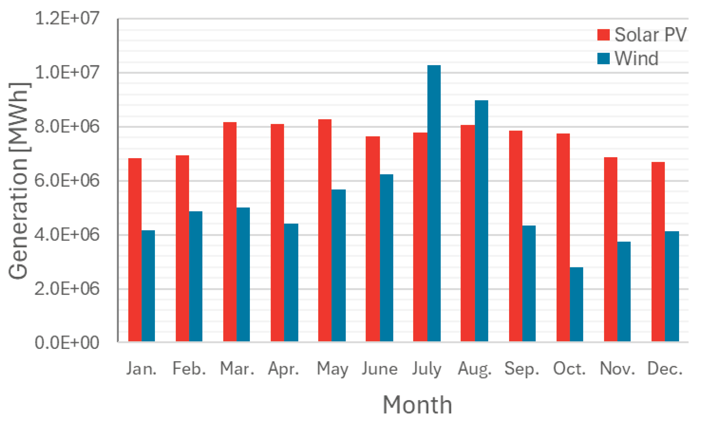
Figure 13.
Hourly performance of an averaged year for the energy sources: a) Solar PV; b) Wind.
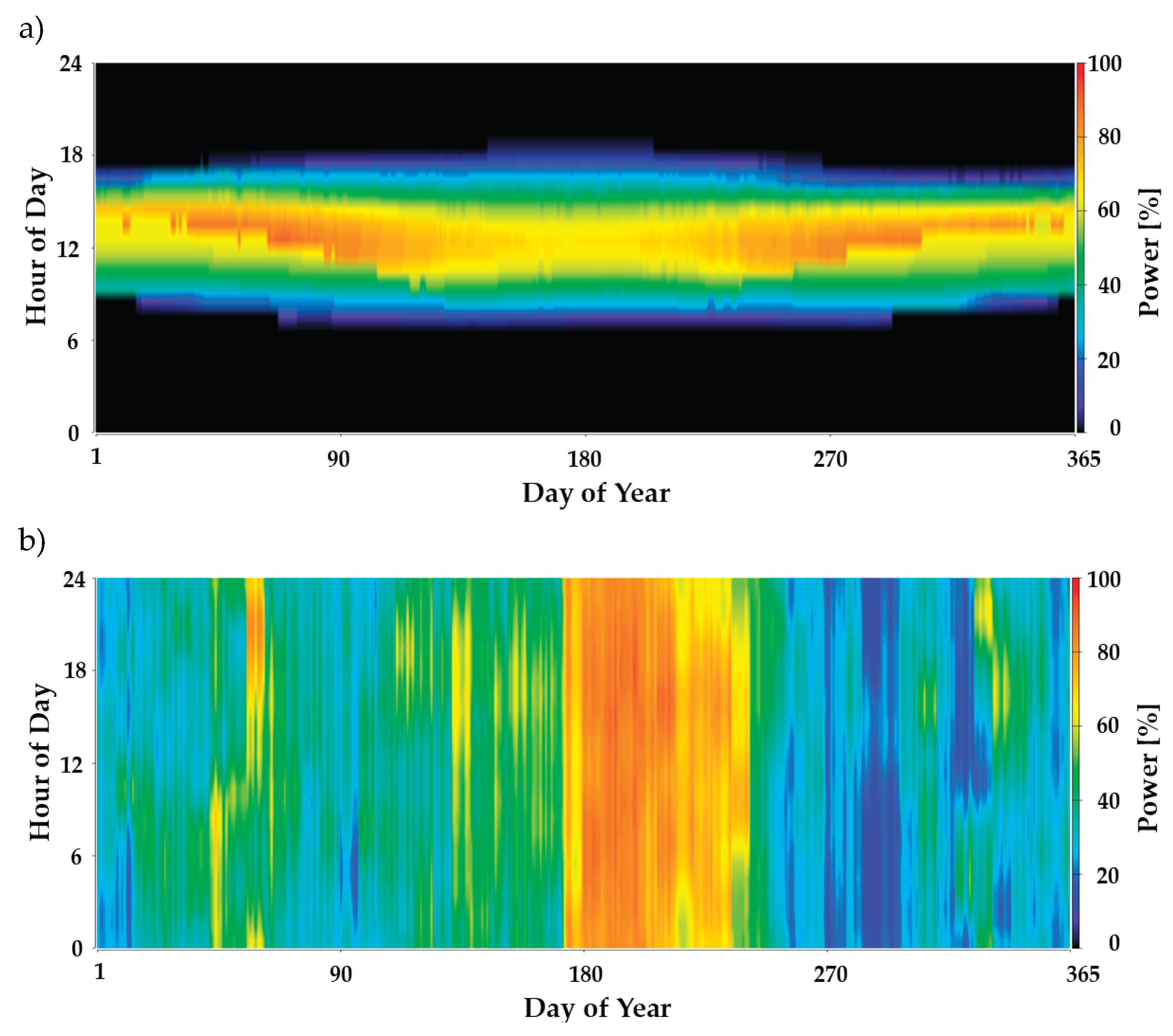
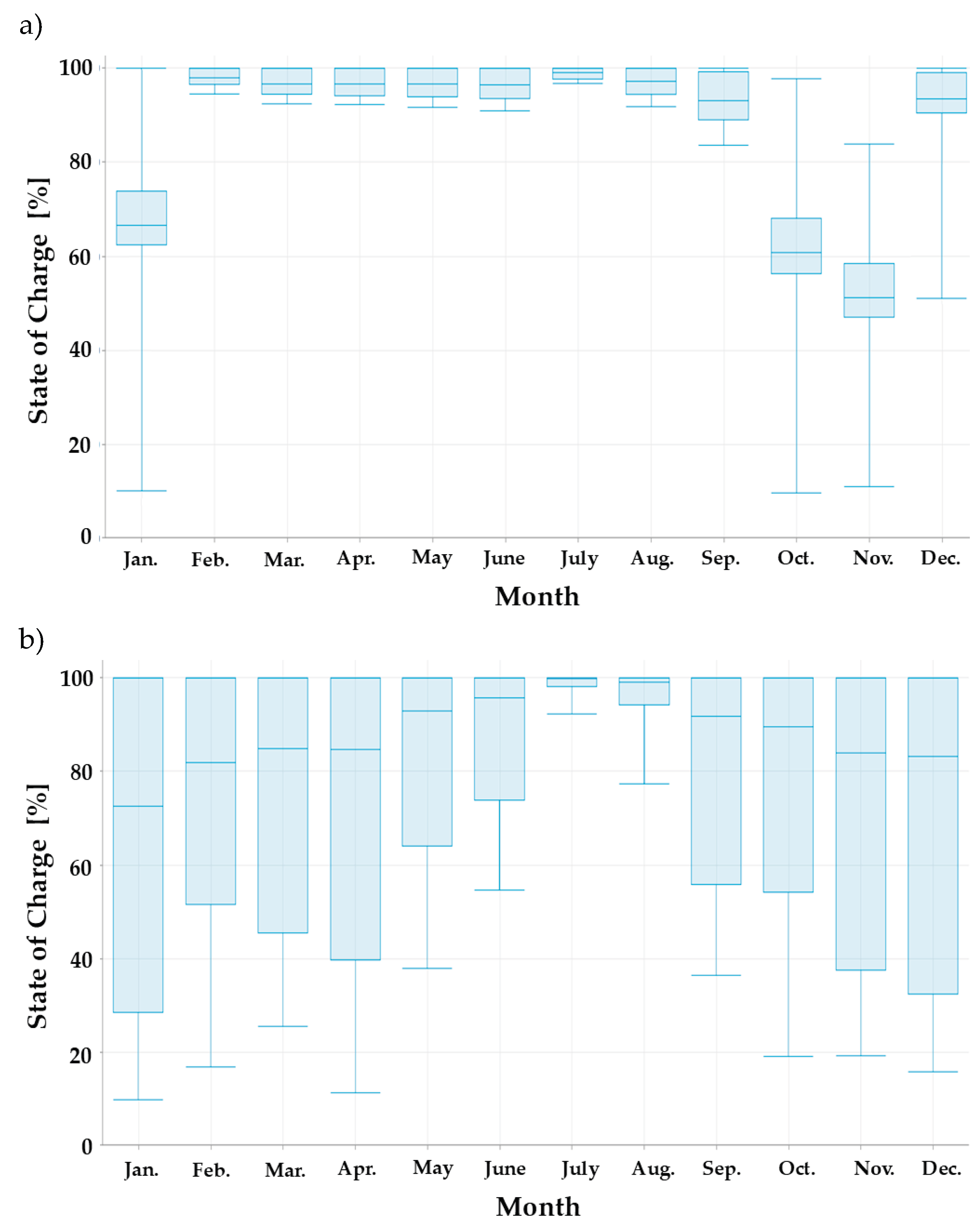
Figure 14 presents the monthly performance (using hourly values in monthly box-and-whisker plots) of the two storage subsystems. Recall that pumped hydro and batteries have storage capacities of 750 MWh and approximately 40 MWh, respectively. Thus, the reversible pumped hydro primarily determines the system’s performance. In any case, as observed in August and especially July, both systems are barely used, with median state of charge (SoC) values close to 100%. At the opposite extreme are October and November, which show the lowest SoCs, with medians around 50% for pumped hydro, and approaching nearly 0% in both cases, January presents a quite similar behaviour, while December is in an intermediate state. Battery SoCs remain higher but also reach minima near 20%. For the other months, the median SoC stays above 90% for pumped hydro and 80% for batteries. This clearly shows that the system operates with a high safety margin every month except for October and especially November. This situation, as will be discussed later, will have significant effects on system reliability when considering uncertainties.
Figure 14.
Monthly performance of an averaged year for the storage systems: a) Reverse Pumping; b) Mega-battery.
Figure 14.
Monthly performance of an averaged year for the storage systems: a) Reverse Pumping; b) Mega-battery.
Concerning the use of the reversible pumped storage system, Figure 15 shows the pumping and turbinating cycles throughout the year. In the pumping refill cycles (Figure 15-a), it is observed that during the summer months there are fewer hours of pumping, with very little pumping occurring, as previously mentioned the system generates energy well above its consumption. For the rest of the year, a higher percentage of pumping occurs during the central hours of the day (the period of maximum solar PV generation).
Regarding the grid injection from reversible pumping, as shown in Figure 15-b, it occurs mainly during the early night hours. During the months less favorable to system performance, turbining is available during the early night hours in the winter months. Although in the summer months, a significant contribution from reversible pumping is not required, the system operates throughout the day except during the central hours, but at relatively low power levels. As seen in Figure 15-c, from approximately day 300 to 330 of the year, the state of charge (SoC) remains very low for extended periods. SoC values are also low just before and just after this period, extending somewhat longer in the latter case.days. The last days of the year and the first ones are also quite low, while for the rest of the year the percentages remain high, showing no critical issues with availability.
Regarding the battery modules (Figure 16), their operation is quite similar to that of reversible pumping, with charging occurring mostly during the central hours of the day (Figure 16-a) and discharging during the night (Figure 16-b). However, in this case, the batteries provide energy to the system frequently during the final hours of the night. For this reason, as shown in Figure 16-c, the batteries reach their lowest SoC during the last hours of the night.
Figure 17 shows the hourly excesses, confirming the general behavior described above. It should be noted that during the worst performance months, there are practically no excesses, with only a few residual excesses occurring around midday during the months of September to December (approximately days 250 to 330). Meanwhile, during the period with the longest days (approximately days 160 to 230), there are excesses during a greater number of hours. Although these excesses show appreciable values shortly after the beginning of the year, they remain from midday until approximately 5 p.m. until approximately day 160. As can be seen in the figure, the excesses are not high (remember excesses of 8%) and are located in specific bands, specifically where solar generation reaches its maximum (remember that installed solar power accounts for more than 75% of the total).
Table 6 presents the key variables related to the financial analysis of the proposed system. Total costs are directly influenced by the installed capacity of each subsystem, establishing a direct link to the data in Table 5, which details electrical generation and power for each system. The total capital expenditure required for the entire electrical installation amounts to just under 150 M€. Within this amount, initial investment accounts for nearly 60%, replacement costs of various subsystems represent 24%, and O&M costs make up approximately the remaining 17%. These combined costs lead to nearly 250 M€ overall, resulting in a final LCOE of 103.0 €/MWh, a value that is currently competitive and likely to remain so through 2040.
Analyzing the costs associated with each subsystem and the different cost components reveals that both solar PV and reverse pumping represent the main contributors to the total system expenditure. However, their cost profiles differ significantly: for solar PV, high replacement costs over the system's lifetime account for a substantial share of the total expenses, whereas in reverse pumping, the initial capital investment dominates the cost structure. In contrast, the mega-batteries subsystem exhibits a relatively low total cost compared to the other subsystems, but most of its expenditure is attributable to periodic replacements, indicating a limited operational life of its main components. The wind generation subsystem, on the other hand, distributes its costs more evenly among capital, replacements, and O&M, though its overall contribution to the total system cost is less significant in absolute terms. Therefore, investment strategies should carefully consider both the heavy upfront capital required for reverse pumping facilities and the substantial replacement needs inherent to PV and battery systems throughout their operational lifecycle.
4.1.2. The Stochastic Approach
As presented in the previous section, a deterministic analysis has yielded a system capable of achieving the established objectives in terms of demand coverage and excess energy control. However, it is obvious that, in practice, the system's performance will not be deterministic. The previous analysis assumed specific hourly generation profiles for both solar and wind resources, as well as unique hourly demand values. In reality, however, the system must be able to meet these objectives under any possible operating condition, given the inherent variability and uncertainty associated with solar PV and wind generation, as well as the stochastic nature of demand. Consequently, the goal is to achieve certain reliability and coverage levels, typically set at 95x95% of confidence and coverage.
To address this challenge, as previously introduced, it is necessary to perform sampling over the probability distribution functions of the uncertain variables, according to the previously described methodology, 93 sampled cases must be defined (93 independent random sampling of the three uncertain variables and over all hours of a year). After conducting such sampling and running the corresponding simulations on the deterministic scenario, a detailed description of the system's behavior under uncertainty is obtained.
The primary variables employed to assess the system’s performance under each scenario are, firstly, the amount of unmet demand—measured as the percentage of load that could not be supplied—and, to a lesser extent, the levels of surplus energy produced by the system. This information is summarized in Figure 18, which displays, for all 93 cases, both the percentage of unmet demand and the proportion of excess electricity.
Upon analyzing the 93 simulated scenarios, several key observations emerge. Of these, only 40 scenarios achieved complete demand coverage at all times. While it is true that most of the 53 scenarios exhibiting unmet demand did so at low levels, it must be acknowledged that any imbalance in a small-scale system can potentially result in a blackout, necessitating careful consideration. The most adverse case exhibits an unmet demand of 1.3%, corresponding to approximately 1.4 GWh per year. At the opposite extreme, the case with total demand coverage also presents the highest energy surplus, constituting about 33% of the total generation. Table 7 summarizes the performance of the three most representative cases: the reference case and the two extreme outcomes derived from uncertainty in solar, wind, and demand inputs. It is worth noting that, across all cases, surplus energy remains contained. This indicates that the system is not significantly oversized, primarily due to the considerable capacity of the two storage subsystems.
However, although most of the 53 cases with unmet demand have a very low percentage, this is not acceptable from the point of view of reliability. Therefore, the system must be resized to eliminate this risk. There are essentially two approaches: (i) upsizing the proposed system, or (ii) implementing an additional dispatchable generation subsystem. If the second solution is preferred, using exclusively renewable sources, the only feasible option given the island’s constraints would be biomass. Alternatively, albeit with higher GHG emissions, the retention of diesel generator sets could be considered. In this latter case, given the low unmet demand percentages, diesel generation would be required rarely, with a capacity factor of only around 1.3% at the 95% reliability and coverage levels.
Exploring different resizing options, offers a general view of the repercussions of uncertainties in the dimensioning of energy systems (Table 8. Performance of possible resized systems in the stochastic approach for the two extreme cases in the BAU scenario). As shown, increasing the battery storage with 21 additional modules (approximately 20 MW of power and nearly 80 MWh of extra storage capacity) would satisfy the reliability requirements. In addition, a substantial increase in solar PV generation—specifically, the installation of 14 MW—would be necessary to ensure demand coverage. Expanding wind generation by adding six extra wind turbines (about 14 MW) was also assessed.
Analyzing the performance of the three options under the most adverse scenario—which motivated the maximum oversizing aimed at ensuring the desired system stability—several key observations can be made. The first option involves the greatest degree of oversizing; however, since it relies solely on storage rather than additional generation sources, it maintains the surplus energy levels of the initial system. The additional installation of solar panels (14 MW) leads to a modest increase of just over 6% in system surpluses. In contrast, increasing the number of wind turbines results in a significant rise in surpluses, approximately 15%, primarily because the most adverse performance period for the system occurred during October and November when wind availability was at its minimum. Finally, the combined configuration of solar and batteries, consisting of a 7 MW peak solar installation and 6 battery modules, produces a moderate increase in surpluses.
Focusing on costs, the lowest LCOE is achieved by the latter option (solar plus batteries), although the re-dimensioned battery system presents a comparable value. In any case, both options incur cost increases exceeding 10% relative to the baseline system identified through deterministic analysis, from the initial 10 c€/kWh generated to more than 11 c€/kWh . The addition of extra wind turbines is the least favorable option from both a cost and surplus energy perspective. While the rise in solar capacity results in costs similar to those of increased wind generation, its surplus levels are closer to those observed for the two options previously identified as most suitable.
It is important to note that the system will not always operate under the most adverse conditions. This implies that, during a favorable year, the system oversizing implemented to ensure reliability under challenging conditions will lead to even greater inefficiency. Consistent with observations in the adverse scenario, wind generation exhibits the poorest performance under favorable conditions, with losses increasing to nearly 50% of the energy generated. The other systems show a contained increase in surpluses, with very similar behavior between the battery-only re-dimensioned system and the hybrid configuration combining batteries and solar PV generation.
Another possibility arises from a detailed analysis of the system’s critical operation intervals revealed that energy deficits occur predominantly during the months of October and November. These shortages are particularly significant, with the system frequently failing to meet the majority of demand during these periods. Specifically, power deficits often exceed 10 MW and can reach instantaneous peaks close to 15 MW. Therefore, if the deployment of a backup generation system is considered, its capacity should be sized according to these maximum observed shortfalls.
4.2. Efficiency Scenario with EV Mobility Policies
As was done for the BAU scenario, in this efficiency scenario the uncertainties associated with the different input variables must be studied. Those associated with both solar and wind resources will be the same as in the BAU scenario. However, in the case of demand, these will differ, not only because of the specific value of the demand, but also because of the different contributions associated with the two fundamental components, i.e., the trend component and the component associated with EVs. Therefore, Figure 19 illustrates the evolution of hourly demand curves during a typical week in winter and summer. It illustrates the projected electricity demand for the 93 cases and the base demand case. The demands predicted by the random sample are shown with lines of different colors, forming a band of demand behavior, while the yellow line represents the base case demand.
As with the BAU scenario, the first iteration starts from a base case, for which the average system conditions presented in Figure 10, Figure 11 and Figure 19 are used (a modeling case that corresponds to a deterministic approach). In a second phase, the intrinsic variability of both renewable generation sources and demand must be considered, using the analyses of the 93 cases described.
4.2.1. The Deterministic Approach
Once again, as with the BAU scenario, the main results of the base case are detailed below. The economic and technical aspects will be considered, analyzed, and discussed, including the different resources considered, specifically wind and solar energy, as well as storage systems. Table 9 presents a summary of the key characteristics of the generation and storage systems. Solar PV generation represents the largest installed capacity, comprising approximately 55% of the total with 42 MW of nominal power, while wind energy accounts for the remaining nearly 45%, around 11.5 MW. The CF for solar PV and wind remains consistent with those reported in the previous section, at nearly 20% and over 45%, respectively. Notably, the system experiences a low percentage of energy surpluses, largely due to the significant role of storage systems, which have a combined power capacity of about 35 MW. As in the prior scenario, the system is capable of absorbing virtually all unused energy, except when the storage units reach full capacity, despite having over 500 MWh of storage available. Additionally, approximately 20% of the demand is supplied back to the grid as needed through the storage systems. The substantial storage capacity effectively reduces energy excesses to around 30% of the total electricity generated.
As for the BAU scenario, Figure 13 and Figure 14 present the solar PV and wind generation. The difference between Figure 12 with the one of this scenario is the installed powers, in this case, these are 42 MW for the solar PV and 11.5 MW for wind generation.
As explained for the BAU scenario (Figure 12 and Figure 13), solar PV generation remains fairly stable throughout the year, with the lowest output during winter months (November to February) and consistent levels otherwise. Wind power generation shows greater variability, peaking in July and August and reaching minimums in October and November, which are the most adverse months due to the combined low output of both resources. Solar energy contributes more in the warmer months, although summer generation is partially reduced by performance losses from high temperatures. Overall, solar remains a key, yet underutilized, renewable resource in El Hierro. Wind generation peaks in summer and dips between mid-September and late November, while maintaining relatively high values during most other months except for some lower production in December, January, and April.
1 Power In/Out refers to the Pumping/Turbination and Charge/Discharge processes for the reverse pumping and batteries, respectively; 2 percentage of energy recovered by the storage systems as a percentage of the total generated energy.
As all the generation graphs are similar to the BAU scenario, merely scaled to the existing capacities, the storage systems exhibit a comparable analogy in their general behavior patterns. Figure 14 and Figure 20 compare reversible pumped storage and battery performance in both scenarios. For the pumped storage systems (Figure 14-a and Figure 20-a), October and November remain the most adverse months, showing the lowest SoC, approaching nearly 0% in both cases. December and January display less extreme behavior in the current scenario than in the BAU; notably, January in BAU has a median SoC around 70% and a minimum near 10%, while the current scenario shows a median above 95% and a minimum not dropping below 90%. December shows a similar trend, though less pronounced: the BAU median is just above 90% with a minimum near 50%; in the current scenario, the median is similar but the minimum is slightly above 80%. For other months, both median and minimum SoC values remain very similar in both scenarios, mostly above 90%; only September has minimum values around 80%, consistent in both scenarios.
Regarding battery behavior (Figure 14-b and Figure 20-b), patterns are similar but with some differences. July and August show lower battery use in both cases, though utilization is lower in BAU (medians near 100% and minima around 90% and 80%, respectively), while in the current scenario, medians are above 90% and minima between 50–60%. For other months, battery use is generally higher in the efficiency scenario than in BAU, with minimum SoC values approaching 0–20% in both, while median SoC values are higher in BAU. Both show increasing battery usage toward winter months, forming an inverted U-shaped trend between January, July, and December—from about 70% to near 100% and back to 80% in BAU, and from 50% to nearly 100% and back to 60% in the current case. These figures clearly indicate that the system operates with a high safety margin every month except October and November. Moreover, weighting their behavior by respective storage capacities would reveal even closer similarities.
Figure 15, Figure 16 and Figure 17 demonstrate nearly identical behavior patterns. The reversible pumped storage system operates with fewer pumping hours in summer, when generation exceeds consumption. Pumping mainly occurs at midday, coinciding with peak solar PV output. Grid injection from pumped storage happens chiefly in early night hours, particularly in winter, to meet demand when renewable generation is low. From days 300 to 330, the SoC remains low for prolonged periods, with similarly low levels before and after this interval, although overall SoC remains high during the rest of the year, indicating strong availability. Battery modules show similar operation, charging around midday and discharging at night, with notable discharge in the final pre-dawn hours, leading to their lowest SoC at that time.
Hourly energy surpluses are minimal during adverse low-generation months (September to December), with only minor midday excesses. During periods with longer daylight (days 160 to 230), surpluses increase but remain moderate (around 8%), concentrated mainly during peak solar generation hours. Overall, both storage systems effectively manage energy flows, minimizing surpluses and maintaining supply consistency throughout the year.
Table 10 summarizes the main financial variables of the proposed system. The total capital expenditure for the entire electrical installation is just under 110 M€. Of this amount, the initial investment represents nearly 60%, replacement costs for the subsystems account for 25%, and O&M costs comprise approximately 17%. Together, these costs total close to 190 million euros, yielding a LCOE of 102.6 €/MWh. The analysis of the associated costs within each subsystem is exactly the same as the description in Table 6, since both systems have the same costs for each technology. However, there are variations in the relative costs of each subsystem, although in both cases solar PV generation systems and irreversible pumping dominate.
4.2.2. The Stochastic Approach
As presented for the BAU scenario, a deterministic analysis results in a system capable of achieving the objectives set in terms of demand coverage and excess energy control, considering the assumptions made, i.e., specific hourly generation profiles for both solar and wind resources, as well as unique hourly demand values. Consequently, a stochastic approach is carried out. This methodology permits the capture of a wide range of possible operational conditions and assesses the robustness of the system’s design.
The primary metric used to evaluate system performance in each scenario is the percentage of unmet demand, that is, the proportion of total load that could not be supplied. A secondary variable of interest is the fraction of surplus energy produced. The results of all 93 scenarios are synthesized in Figure 21, which shows, for each case, both the unmet demand percentage and the proportion of surplus electricity.
Analysis of these 93 simulated scenarios reveals several important insights. Notably, only 33 scenarios resulted in complete satisfaction of demand throughout the year. Although unmet demand in the remaining 60 cases was generally low, it is important to recognize that even small mismatches can be dangerous in a microgrid or small-scale system, as any shortfall may lead to potential zero energy supplies. The most severe case observed showed an unmet demand of nearly 1.3%, equating to approximately 1.07 GWh annually. In contrast, the scenario that achieved full demand coverage also exhibited the highest level of surplus generation, with excess electricity reaching more than 12% of total annual production.
Table 11. Performance of the optimized deterministic system over a stochastic approach for the Efficiency scenario. provides a summary of the performance observed in the three most representative scenarios: the reference case, and the two extreme outcomes reflecting the greatest impact of uncertainties in solar, wind, and demand data. Across all scenarios, it is notable that the volume of surplus energy remains limited, which suggests that the system is well-sized—neither significantly oversized nor undersized—thanks largely to the substantial storage capacity provided by the two storage subsystems.
The same considerations applied to the BAU scenario also hold in the Efficiency scenario, with the only difference being that the solar generation system must be greatly expanded in order to meet the demand of the more restrictive case (power increase of 32 MW). This situation is driven by the fact that this Efficiency scenario features a reduced storage capacity, which is unable to redistribute solar surpluses during critical periods, resulting in significantly more adverse system performance. Therefore, this option should be discarded in this case, leaving the two options identified as most suitable in the BAU scenario—the increased battery system and the hybrid configuration combining a modest increase in solar PV with battery storage—as the preferred choices.
In this Efficiency scenario, similar observations to those made for the BAU scenario can be drawn. Specifically, eliminating the lack of coverage by resizing the system—through significant increases in power capacity and/or storage—requires very substantial upgrades. As in the BAU scenario, these big demands cluster in the system’s most challenging performance intervals, during which almost no energy demand can be met. Therefore, the most appropriate solution is likely the implementation of a backup system, which under the most unfavorable conditions would generate around 1% of the annual energy demand. Its capacity would need to be close to the peak demand power, estimated in this scenario to be approximately 10–12 MW.

Table 12.
Performance of possible resized systems in the stochastic approach for the two extreme cases in the Efficiency scenario
Table 12.
Performance of possible resized systems in the stochastic approach for the two extreme cases in the Efficiency scenario
| Resized Solar PV | Resized Wind | Resized Batteries | Resized Solar PV/Batteries | ||||||
|---|---|---|---|---|---|---|---|---|---|
| Unfavour. Case | Favou. Case | Unfavour. Case | Unfavour. Case | Unfavour. Case | Favour. Case | Unfavour. Case | Favour. Case | ||
| Resizing (MW) | 32 MW PV Pannels | 5 Wind Turbines (11.5 MW) | 17 Batt (16.64MW, 66.57MWh) | 6 MW PV / 4 Batt (3.916MW, 15.66MWh) | |||||
| Generation (GWh) | 175.83 | 178.87 | 169.75 | 175.82 | 120.91 | 123.95 | 131.21 | 134.25 | |
| Generation Surpluses (GWh) | 86.33.08 | 90.26 | 81.65 | 88.70 | 31.04 | 38.66 | 42.58 | 46.44 | |
| (%) | 46.2 | 47.80 | 45.70 | 48.40 | 28.50 | 30.90 | 30.4 | 32.7 | |
| System Costs (M€) | 248.91 | 248.72 | 210.90 | 210.65 | 204.74 | 204.56 | 201.51 | 201.32 | |
| LCOE (c€/kWh) | 13.38 | 13.71 | 11.59 | 11.61 | 11.25 | 11.27 | 11.08 | 11.09 | |
4.3. Key Findings on Renewable Integration Improvement and Uncertainty Assessment
The ambitious decarbonization targets of the European Union have propelled Spain, particularly its non-mainland territories, to advance rapid energy transitions. The Canary Islands Energy Transition Plan (PTECan) aims to achieve full economic decarbonization by 2040, a decade earlier than the national target. This study projects a system designed to meet all energy demands through a GHG-free mix, relying exclusively on renewable generation supported by energy storage systems for the island of El Hierro.
Analyses have highlighted the challenges faced by isolated regions such as islands and remote areas, which must operate as self-sufficient systems. These regions typically depend on fossil fuels to maintain the necessary reliability and stability, since renewables alone cannot consistently meet energy needs directly.
The two projected scenarios evaluate energy systems designed to meet the full spectrum of the island’s energy demands by 2040 through an integrated mix of renewable technologies, encompassing the upper and lower bounds of anticipated demand under a comprehensive economic electrification trajectory. The lower-bound scenario anticipates approximately a 60% increase over current demand, leading to close to 85 GWh per year. While the upper-bound scenario expects demand to nearly double, up to more than 105 GWh poer year. One scenario follows a baseline path of gradual evolution, with the primary disruptive change being the full penetration of EVs. In contrast, the other envisions a more transformative future driven by stringent efficiency improvements and strong policies favoring collective transportation. Together, these scenarios represent the extreme trajectories of system evolution, offering valuable insights and guidelines for guiding the necessary paradigm shift in electricity generation and demand as the island transitions toward 2040.
In both scenarios, the solar PV subsystem, representing about 75% of installed capacity and approximately 60% of electrical generation, is justified by its relatively low cost. The design emphasizes self-consumption, utilizing the large available surface area on the island while avoiding large-scale solar farms to minimize land use and visual impact—an important consideration for islands with significant tourism sectors. Although high solar PV integration carries risks such as electrical system oversizing and increased energy surpluses due to generation variability, these challenges necessitate complementary systems to maintain balance.
Wind generation holds a significant role due to the high capacity factors achievable in the Canary Islands, particularly for offshore installations, currently around 45%. Despite inherent variability, local conditions yield relatively stable generation. Thus, wind contributes roughly 40% of generation, with installed capacity approximately 25% of the system total. Specific local constraints and existing infrastructure—currently including five wind turbines on the island—have informed site selection and system design.
The substantial power and energy capacity of the storage subsystems—recharge power on the order of 60% of installed generating capacity and storage capacity approximately 40 times the island’s peak power demand—enhances system flexibility notably. These storage units effectively absorb excess energy during overgeneration periods, accounting for around 20% of total generated energy, and return it to the grid as needed.
The energy surplus within the proposed system remains relatively low—around 30%—which is efficient given the scale of the scenario. This performance is largely attributable to the substantial storage capacity provided by the combined reverse pumping and megabattery subsystems, which effectively absorb excess generation and thereby minimize overall energy wastage.
The BAU scenario comprises solar PV (power of 53 MW) and wind (16 MW). Large storage systems (over 40 MW power, ~800 MWh capacity) absorb most excess energy, keeping surpluses to about 27% of total generation. Storage includes pumped hydro (32 MW, 750 MWh, 81% efficiency) and batteries (nearly 10 MW, 39 MWh, 94% efficiency). This mix ensures efficient use of renewable energy and system flexibility.
In the Efficiency scenario, the generation mix consists of about 42 MW of solar PV and 11.5 MW. Storage systems have a combined power capacity of approximately 35 MW and 539 MWh of energy storage, including pumped hydro (25 MW, 500 MWh) and batteries (around 10 MW, 39 MWh).
The LCOE for both resulting energy mixes is relatively low, slightly above 100 €/MWh, making it cost-competitive. Cost analysis identifies solar PV energy and pumped hydro storage as the primary contributors to total system expenditure, although with distinct cost profiles: PV systems incur substantial replacement costs over their lifetime, whereas pumped hydro is characterized by high upfront capital investment. Megabatteries exhibit relatively low total costs but require frequent replacements due to the limited lifespan of their components. Wind generation costs are more evenly distributed among capital, O&M, and replacements, but their overall contribution to total cost is smaller. Hence, investment strategies should balance the high initial capital of pumped storage against ongoing replacement needs for solar PV and battery systems during their operational life.
Uncertainty analysis considering the inevitable variability of solar and wind resources, as well as demand, revealed a significant impact on system self-sufficiency. The results demonstrate the need to oversize generation and storage systems to cope with these fluctuations. Simulations of multiple stochastic scenarios suggest that while a deterministic system may meet coverage and surplus control targets, variability and uncertainty in renewable generation and demand often lead to incomplete demand coverage, typically with small deficits. Increases of at least 10% in installed power generation are needed, leading to cost increases of approximately 110 €/MWh.
In the most adverse case of the BAU scenario, oversizing the system by adding storage alone maintains surplus energy levels comparable to those of the original system. Adding 14 MW of solar panels modestly increases surpluses by just over 6%, while expanding wind turbine capacity causes a larger surplus increase of approximately 15%, primarily due to low wind availability during critical system performance months (October and November). The combined option of 7 MW solar PV plus battery modules results in a moderate increase in surplus and achieves the lowest LCOE; however, all oversizing options raise costs by over 10% compared to the baseline system. Among the three, adding wind turbines is the least favorable option considering both cost and surplus energy.
Under more favorable conditions, system oversizing leads to increased inefficiencies, particularly for wind generation, which can lose nearly 50% of its generated energy. Other configurations show smaller increases in surplus energy, with very similar behavior between the battery-only and the solar-plus-battery re-dimensioned systems.
A backup generation system sized near the peak demand (about 15 MW) would be another option to manage system oversizing and ensure reliability under challenging conditions. This backup would supply about 1.4% of the annual energy demand. On El Hierro Island, biomass is essentially the only available renewable option for such backup generation, providing a dispatchable, sustainable complement to wind, solar PV, and pumped hydro storage. Integrating biomass-based backup enhances system stability and supports the island’s high renewable energy penetration goals.
In the Efficiency scenario, the trends are similar, but a substantially larger increase in solar capacity (about 32 MW) is required to meet the stricter demand due to reduced storage capacity. This limited storage cannot effectively redistribute solar surpluses during mainly during high solar PV periods, resulting in poorer system performance. Consequently, relying solely on expanded solar generation is not advisable in this scenario. The preferred options remain those identified in the BAU scenario: increased battery capacity alone or combined with a moderate increase in solar PV. As for the BAU scenario, the possibility to use a backup system is open; in this case, about 10-12 MW of installed power would be needed, covering up to about 1 GWh per year under the most adverse forecasted conditions.
To cover persistent demand gaps, substantial system upgrades or the integration of a backup generation system sized near peak demand—estimated at 10 to 12 MW—would be necessary. This backup would supply approximately 1% of the annual energy demand, providing an important reliability measure under the most challenging conditions.
These findings indicate the current system, without adjustment, carries an unacceptable reliability risk, particularly in small-scale systems where imbalances can lead to outages. To mitigate this risk, two main strategies emerge: increasing system capacity (generation and/or storage) or incorporating dispatchable generation to cover periods. Among renewable options, biomass presents a viable backup solution.
Adjustments combining moderate increases in renewable generation and storage yield a system capable of meeting demand without excessive oversizing and with reasonable control of surpluses.
Finally, the higher deficit periods have been identified during specific times of the year, enabling the appropriate sizing of backup generation to ensure reliability when it is most needed.
These outcomes underline the complexity of designing a fully renewable energy system in isolated regions like El Hierro. Achieving a balance between renewable generation, storage, and backup systems—while minimizing or eliminating dependency on fossil fuels—is essential to controlling costs and achieving environmental goals. The application of advanced optimization tools and real-world case studies underscores the importance of meticulous system planning to achieve energy independence, grid stability, and decarbonization under challenging conditions.
Potential future research directions include investigating the impact of demand management policies, Vehicle-To-Grid (V2G) and Vehicle-To-Home (V2H) technologies. Exploring measures that align demand profiles with generation availability by encouraging consumption at optimal times, as well as leveraging EVs as flexible energy sources or loads, could further support self-consumption and enhance energy efficiency.
5. Conclusions
The transition toward fully decarbonized energy systems in isolated territories, such as the Canary Islands and specifically El Hierro, requires carefully designed solutions that balance generation, storage, and system reliability under variable and uncertain conditions.
Major findings and system characteristics of the current study are:
- System Composition & Cost Efficiency. The proposed systems combine high shares of renewable generation—primarily solar PV and wind—with substantial storage capacity (including pumped hydro and megabatteries). The resulting levelized cost of energy (~100 €/MWh) is competitive, with relatively rapid payback, demonstrating economic viability.
- Renewable Generation Roles and Constraints. Solar PV generally constitutes the majority of installed capacity and generation due to its cost-effectiveness and extensive self-consumption potential on available land. However, careful planning is needed to mitigate oversizing and resultant excess generation caused by the inherent intermittency. Wind energy contributes significantly, supported by favorable capacity factors, especially offshore. Its inclusion improves generation stability despite site-specific environmental and regulatory constraints.
- Storage and Flexibility. Large-scale storage assets, principally reversible pumped hydro complemented by battery systems, provide essential flexibility by absorbing excess energy and releasing it when needed. This effectively limits energy waste to below 10% of total generation—an efficient outcome for a system of this scale.
- System Reliability and Uncertainty. Stochastic analyses reveal that variability and uncertainty in renewable generation and demand introduce non-negligible risks of unmet demand, which, while often small, remain unacceptable for reliable system operation. To mitigate this, the system must either be upsized in generation and storage capacity or supplemented with dispatchable backup generation. Biomass emerges as a renewable backup option fitting local constraints, whereas limited and rare use of diesel generators could also maintain stability, albeit with higher emissions.
- Optimized System Adjustments. Moderate simultaneous increases in renewable generation and storage capacities offer a balanced solution, improving reliability without excessive oversizing or surplus energy increase. Temporal analysis of deficits identifies specific periods of highest vulnerability, enabling the targeted sizing of backup systems to effectively cover peak shortfalls.
- Investment Considerations. Cost structures vary among components: the solar PV system incurs substantial long-term replacement costs, pumped hydro storage requires high initial capital investment, and battery systems have moderate costs but limited lifespans requiring periodic replacements. Wind offers a balanced cost profile but constitutes a smaller share of total expenditure. Investment strategies must account for these differing profiles to optimize lifecycle costs and operational reliability.
- System Integration and Interconnection. Consolidating multiple island grids via interconnections enhances overall system flexibility and performance, allowing energy sharing, better surplus management, and improved reliability.
Major future research directions could cover:
- Advanced Demand Management. Development and assessment of policies and demand response strategies that better align consumption with renewable generation profiles.
- Exploration of Vehicle-To-Grid (V2G), Vehicle-To-Home (V2H), Vehicle-To-Building (V2B), and Vehicle-To-Load (V2L) technologies to utilize electric vehicles as flexible energy assets for grid balancing, peak shaving, and backup.
- Smart Systems and Control. Integration of smart charging infrastructure with predictive analytics and AI to optimize energy use, reduce costs, and enhance grid stability.
- Hybrid Storage and Generation Synergies. Studying the combined use of different storage technologies (hydro, batteries, hydrogen) to optimize cost, reliability, and environmental impact.
- Evaluating DSM in concert with distributed renewables and storage to minimize curtailments.
- Long-term impacts of widespread EV-based storage on infrastructure, lifecycle performance, and sustainability.
- Policy and Consumer Engagement. Examination of incentives fostering consumer participation in flexibility markets and self-consumption.
- Strategies to promote energy efficiency and the alignment of demand patterns with renewable availability.
Author Contributions
Lucas Álvarez-Piñeiro (LAP), César Berna-Escriche (CBE), Paula Bastida-Molina (PBM), David Blanco-Muelas (DBM). Conceptualization, LAP, CBE, DBM.; methodology, LAP, CBE, PBM, DBM; software, LAP, DBM; validation, LAP, CBE, PBM, DBM; formal analysis, CBE, LAP, PBM; investigation, CBE, LAP, DBM; resources, CBE, DBM and LAP; data curation, CBE., LAP, DBM; writing—original draft preparation, CBE, LAP; writing—review and editing, PBM, DBM; visualization, CBE, LAP.; supervision, CBE, PBM.; project administration, CBE., PBM.; funding acquisition, CBE, PBM. All authors have read and agreed to the published version of the manuscript.
Funding
This research received no external funding.
Data Availability Statement
Data will be provided upon request.
Acknowledgments
We would like to thank our colleagues at IIE and DEIOAC for their invaluable support and collaboration, which have contributed significantly to the achievement of this work.
Conflicts of Interest
The authors declare no conflicts of interest.
References
- IEA-International Energy Agency, World Energy Outlook 2023, 2023. https://www.iea.org/reports/world-energy-outlook-2023?wpappninja_v=2hxmmubob (accessed May 26, 2025).
- International Energy Agency, Global Energy Review 2021 Assessing the effects of economic recoveries on global energy demand and CO2 emissions, 2021. www.iea.org/t&c/.
- BP, Energy Outlook 2022 edition, 2022. https://www.bp.com/content/dam/bp/business-sites/en/global/corporate/pdfs/energy-economics/energy-outlook/bp-energy-outlook-2022.pdf (accessed September 19, 2024).
- IRENA, Renewable Power Generation, Costs in 2022, 2023. www.irena.org.
- I. Capellán-Pérez, M. Mediavilla, C. de Castro, Ó. Carpintero, L.J. Miguel, Fossil fuel depletion and socio-economic scenarios: An integrated approach, Energy 77 (2014) 641–666. [CrossRef]
- K. Whiting, L.G. Carmona, T. Sousa, A review of the use of exergy to evaluate the sustainability of fossil fuels and non-fuel mineral depletion, Renewable and Sustainable Energy Reviews 76 (2017) 202–211. [CrossRef]
- J. Lin, X. Wang, Q. Yang, A consensus-based algorithm for electric vehicle charging system, in: 2020 IEEE 4th Conference on Energy Internet and Energy System Integration: Connecting the Grids Towards a Low-Carbon High-Efficiency Energy System, EI2 2020, Institute of Electrical and Electronics Engineers Inc., 2020: pp. 4403–4406. [CrossRef]
- S.T. Henriques, K.J. Borowiecki, The drivers of long-run CO2 emissions in Europe, North America and Japan since 1800, Energy Policy 101 (2017) 537–549. [CrossRef]
- C. Berna-Escriche, Á. Pérez-Navarro, A. Escrivá, E. Hurtado, J.L. Muñoz-Cobo, M.C. Moros, Methodology and application of statistical techniques to evaluate the reliability of electrical systems based on the use of high variability generation sources, Sustainability (Switzerland) 13 (2021). [CrossRef]
- UNECE - United Nations Economic Commission for Europe, Carbon Neutrality in the UNECE Region: Integrated Life-cycle Assessment of Electricity Sources, 2022. https://unece.org/documents/2022/08/integrated-life-cycle-assessment-electricity-sources (accessed May 26, 2025).
- Y. Rivera, D. Blanco, P. Bastida-Molina, C. Berna-Escriche, Assessment of a Fully Renewable System for the Total Decarbonization of the Economy with Full Demand Coverage on Islands Connected to a Central Grid: The Balearic Case in 2040, Machines 11 (2023) 782. [CrossRef]
- European Commission, Strategic Energy Technology Plan, (2023). https://energy.ec.europa.eu/topics/research-and-technology/strategic-energy-technology-plan_en (accessed July 21, 2024).
- A. Ioannidis, K.J. Chalvatzis, Energy Supply Sustainability for Island Nations: A Study on 8 Global Islands, in: Energy Procedia, Elsevier Ltd, 2017: pp. 3028–3034. [CrossRef]
- F. Dellano-Paz, A. Calvo-Silvosa, S. Iglesias Antelo, I. Soares, The European low-carbon mix for 2030: The role of renewable energy sources in an environmentally and socially efficient approach, Renewable and Sustainable Energy Reviews 48 (2015) 49–61. [CrossRef]
- C. Vargas-Salgado, C. Berna-Escriche, A. Escrivá-Castells, D. Alfonso-Solar, Optimization of the electricity generation mix using economic criteria with zero-emissions for stand-alone systems: Case applied to Grand Canary Island in Spain, Progress in Nuclear Energy 151 (2022). [CrossRef]
- Y. Rivera-Durán, C. Berna-Escriche, Y. Córdova-Chávez, J.L. Muñoz-Cobo, Assessment of a Fully Renewable Generation System with Storage to Cost-Effectively Cover the Electricity Demand of Standalone Grids: The Case of the Canary Archipelago by 2040, Machines 11 (2023) 101. [CrossRef]
- M. Huber, D. Dimkova, T. Hamacher, Integration of wind and solar power in Europe: Assessment of flexibility requirements, Energy 69 (2014) 236–246. [CrossRef]
- C. Berna-Escriche, Y. Rivera, L. Alvarez-Piñeiro, J.L. Muñoz-Cobo, Best estimate plus uncertainty methodology for forecasting electrical balances in isolated grids: The decarbonized Canary Islands by 2040, Energy 294 (2024). [CrossRef]
- D. Blanco, Y. Rivera, C. Berna-Escriche, J.L. Muñoz-Cobo, Economy decarbonization using green hydrogen and electricity, forecasts and sensitivity analysis for the Canarian Islands in 2040, J Energy Storage 80 (2024) 110232. [CrossRef]
- M. Amir, R.G. Deshmukh, H.M. Khalid, Z. Said, A. Raza, S.M. Muyeen, A.S. Nizami, R.M. Elavarasan, R. Saidur, K. Sopian, Energy storage technologies: An integrated survey of developments, global economical/environmental effects, optimal scheduling model, and sustainable adaption policies, J Energy Storage 72 (2023). [CrossRef]
- C. Berna-Escriche, C. Vargas-Salgado, D. Alfonso-Solar, A. Escrivá-Castells, Can a fully renewable system with storage cost-effectively cover the total demand of a big scale standalone grid? Analysis of three scenarios applied to the Grand Canary Island, Spain by 2040, J Energy Storage 52 (2022). [CrossRef]
- E.I. and G. de C. Cabildo El Hierro, Gorona del Viento - El Hierro S.A., (2016). https://www.goronadelviento.es/en/ (accessed October 16, 2025).
- Alberto Amores, Laureano Álvarez, Joaquín Chico, Gonzalo Ramajo, Ana Márquez, Álvaro Benito, A smart transition to a sustainable energy model for Spain in 2050: energy efficiency and electrification (Spanish “Una transición inteligente hacia un modelo energético sostenible para España en 2050: la eficiencia energética y la electrificación”), 2018. https://www.gasnam.es/wp-content/uploads/2018/01/Deloitte-ES-MonitorDeloitte-Modelo-energetico-Espana-2050-enero-2018.pdf (accessed May 26, 2025).
- Ministerio para la Transición Energética y el Reto Demográfico, PNIEC 2023-30 Borrador para la actualización del PNIEC 2023-2030-64347, 2023. https://www.miteco.gob.es/es/energia/participacion/2023-y-anteriores/detalle-participacion-publica-k-607.html (accessed June 12, 2024).
- Monitor Deloitte, Los Territorios No Peninsulares 100% descarbonizados en 2040: la vanguardia de la transición energética en España, 2020.
- Instituto Tecnológico de Canarias, PTECan - Plan de Transición Energética de Canarias, 2023. https://www.gobiernodecanarias.org/energia/descargas/SDE/Portal/PTECan2030_VI/1-VersionInicial_PTECan_diligenciado.pdf (accessed May 19, 2025).
- Gobierno de Canarias, Anuario Energético de Canarias 2022, 2024. https://www.gobiernodecanarias.org/energia/descargas/SDE/Portal/Publicaciones/AnuarioEnergeticodeCanarias_2022.pdf (accessed May 15, 2024).
- C. Berna-Escriche, C. Vargas-Salgado, D. Alfonso-Solar, A. Escrivá-Castells, Hydrogen Production from Surplus Electricity Generated by an Autonomous Renewable System: Scenario 2040 on Grand Canary Island, Spain, Sustainability 14 (2022) 11884. [CrossRef]
- Y. Rivera, C. Berna-Escriche, Y. Córdova-Chávez, L. Álvarez-Piñeiro, D. Blanco, Forecasts for full decarbonization of the economy in off-grid systems with high end-use consumption rates through combined electricity and hydrogen deployment, the Canary Islands in 2040, J Energy Storage 114 (2025). [CrossRef]
- L. Álvarez-Piñeiro, Y. Rivera, C. Berna-Escriche, D. Blanco, Formulation of best estimate plus uncertainty methodologies for economy decarbonization in high-energy-demand isolated systems: Canary Islands forecasts for 2040, Energy Convers Manag 314 (2024). [CrossRef]
- F.J. Garcia Latorre, J.J. Quintana, I. de la Nuez, Technical and economic evaluation of the integration of a wind-hydro system in El Hierro island, Renew Energy 134 (2019) 186–193. [CrossRef]
- Red Eléctrica de España (REE), Esios - Demanda de El Hierro, (2025). https://www.esios.ree.es/es/analisis/1344?vis=1&start_date=03-06-2024T00%3A00&end_date=03-06-2024T23%3A55&compare_start_date=02-06-2024T00%3A00&groupby=hour (accessed June 3, 2024).
- UNESCO, El Hierro - Reserva Mundial de la Biosfera, (n.d.). https://reservabiosferaelhierro.com/ (accessed October 16, 2025).
- Endesa, Declaracióm Ambiental - CD Lllanos Blancos, 2019.
- Gorona del Viento El Hierro S.A., Declaración Ambiental, 2022.
- H.K. Ringkjøb, P.M. Haugan, I.M. Solbrekke, A review of modelling tools for energy and electricity systems with large shares of variable renewables, Renewable and Sustainable Energy Reviews 96 (2018) 440–459. [CrossRef]
- M.G. Prina, D. Groppi, B. Nastasi, D.A. Garcia, Bottom-up energy system models applied to sustainable islands, Renewable and Sustainable Energy Reviews 152 (2021). [CrossRef]
- NREL, HOMER ENERGY, (2020). https://www.homerenergy.com/ (accessed September 13, 2024).
- S. Bahramara, M.P. Moghaddam, M.R. Haghifam, Optimal planning of hybrid renewable energy systems using HOMER: A review, Renewable and Sustainable Energy Reviews 62 (2016) 609–620. [CrossRef]
- Wald A., An extension of wilks’ method for setting tolerance limits_1177731491, Columbia University (1943).
- Wilks S. S., Determination of sample sizes for setting tolerance limits, Princeton University (1941).
- R. Alzbutas, E. Norvaisa, Uncertainty and sensitivity analysis for economic optimisation of new energy source in Lithuania, Progress in Nuclear Energy 61 (2012) 17–25. [CrossRef]
- European Commission, Photovoltaic Geographical Information System (PVGIS), (2025). https://re.jrc.ec.europa.eu/pvg_tools/en/ (accessed April 11, 2025).
- W. Härdle, J. Horowitz, J.P. Kreiss, Bootstrap methods for time series, International Statistical Review 71 (2003) 435–459. [CrossRef]
- Instituto Tecnológico de Canarias, Manageable Generation Strategy (Spanish “Estrategia de la Generación Gestionable”), Las Palmas de Gran Canaria, 2022. https://www.gobiernodecanarias.org/energia/materias/planificacion/ (accessed May 12, 2025).
- Instituto Tecnológico de Canarias, Canary Islands Strategy for Demand Management and Smart Grids (Spanish “Estrategia Canaria de Gestión de Demanda y Redes Inteligentes”), Las Palmas de Gran Canaria, 2022. https://www.gobiernodecanarias.org/energia/materias/planificacion/ (accessed May 12, 2025).
- Instituto Tecnológico de Canarias, Estrategia del Vehículo Eléctrico, Las Palmas de Gran Canaria, 2021. https://www.gobiernodecanarias.org/energia/materias/planificacion/ (accessed December 11, 2023).
- Gobierno de Canarias, ISTAC - Instituto Canario de Estadística, (2024). https://www3.gobiernodecanarias.org/aplicaciones/appsistac/jaxi-istac/tabla.do?uripx=urn:uuid:31730d2f-86a8-4f0b-a706-5e5942702b7b&uripub=urn:uuid:172cc83a-4789-4f72-bf57-a4d0147c0656 (accessed May 30, 2024).
- X. Li, Z. Wang, L. Zhang, Z. Huang, F. Guo, A. Sivakumar, D.U. Sauer, Electric vehicle charging flexibility assessment for load shifting based on real-world charging pattern identification, ETransportation 23 (2025). [CrossRef]
- Dirección General de Tráfico, La DGT en cifras resultados, (2021). https://www.transportes.gob.es/carreteras/nuestra-red/movilidad/estimacion-trafico-rce-datos-provisionales (accessed February 25, 2025).
- T. Terlouw, C. Bauer, R. McKenna, M. Mazzotti, Large-scale hydrogen production via water electrolysis: a techno-economic and environmental assessment, Energy Environ Sci 15 (2022) 3583–3602. [CrossRef]
- Enercon, Enercon Product Portfolio - E70 E4, (2024). https://pdf.archiexpo.es/pdf-en/enercon/data-sheets-enercon/88093-354545.html#open969034 (accessed May 20, 2024).
- Instituto Tecnológico de Canarias, Estrategia para el Autoconsumo Fotovoltaico, Las Palmas de Gran Canaria, 2021. https://www.gobiernodecanarias.org/energia/materias/planificacion/ (accessed May 12, 2025).
- Trina Solar, Vertex 550W+, (2022). https://static.trinasolar.com/sites/default/files/BrochureVertex550W-EN.pdf (accessed October 14, 2022).
- Instituto Tecnológico de Canarias, Estrategia del Almacenamiento Energético, Las Palmas de Gran Canaria, 2021. https://www.gobiernodecanarias.org/energia/materias/planificacion/ (accessed May 12, 2025).
- C. Berna-Escriche, L. Álvarez-Piñeiro, D. Blanco, Y. Rivera, Optimizing Sustainable Energy Transitions in Small Isolated Grids Using Multi-Criteria Approaches, Applied Sciences (Switzerland) 15 (2025). [CrossRef]
- Tesla (c) 2025, Megapack 2 XL Datasheet, (n.d.). https://www.tesla.com/megapack (accessed April 10, 2025).
- Endesa, El Hierro, an example of sustainability, (2023).
- M.G. Prina, M. Cozzini, G. Garegnani, G. Manzolini, D. Moser, U. Filippi Oberegger, R. Pernetti, R. Vaccaro, W. Sparber, Multi-objective optimization algorithm coupled to EnergyPLAN software: The EPLANopt model, Energy 149 (2018) 213–221. [CrossRef]
- R. Segurado, G. Krajačić, N. Duić, L. Alves, Increasing the penetration of renewable energy resources in S. Vicente, Cape Verde, Appl Energy 88 (2011) 466–472. [CrossRef]
- N.H. Mirjat, M.A. Uqaili, K. Harijan, G. Das Walasai, M.A.H. Mondal, H. Sahin, Long-term electricity demand forecast and supply side scenarios for Pakistan (2015–2050): A LEAP model application for policy analysis, Energy 165 (2018) 512–526. [CrossRef]
- L.M.H. Hall, A.R. Buckley, A review of energy systems models in the UK: Prevalent usage and categorisation, Appl Energy 169 (2016) 607–628. [CrossRef]
- Homer Energy, HOMER Pro 3.14 User Manual, (2020). https://homerenergy.com/products/pro/docs/ (accessed December 14, 2023).
- Instituto Tecnológico de Canarias, Estrategia de las Energías Renovables Marinas, Las Palmas de Gran Canaria, 2022. https://www.gobiernodecanarias.org/energia/materias/planificacion/ (accessed May 12, 2025).
- Instituto Tecnológico de Canarias, Canary Islands Green Hydrogen Strategy (Spanish “Estrategia Canaria del Hidrógeno Verde”), Las Palmas de Gran Canaria, 2022. https://www.gobiernodecanarias.org/energia/materias/planificacion/ (accessed May 15, 2024).
Figure 1.
Electric demand curve of the El Hierro island.
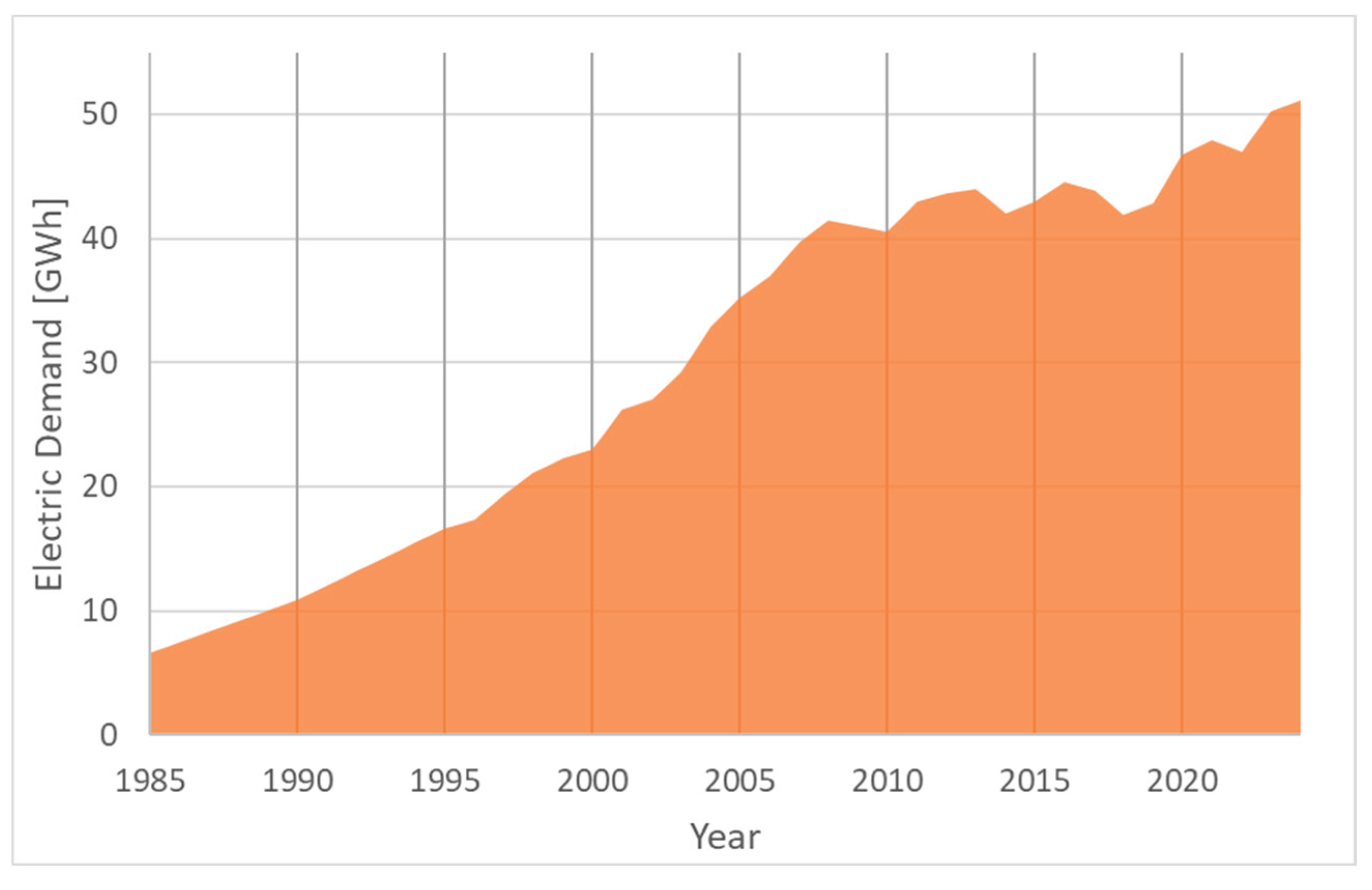
Figure 2.
Monthly profiles of daily and hourly electricity demand curves for a typical year (specifically, the displayed data are from 2023).
Figure 2.
Monthly profiles of daily and hourly electricity demand curves for a typical year (specifically, the displayed data are from 2023).
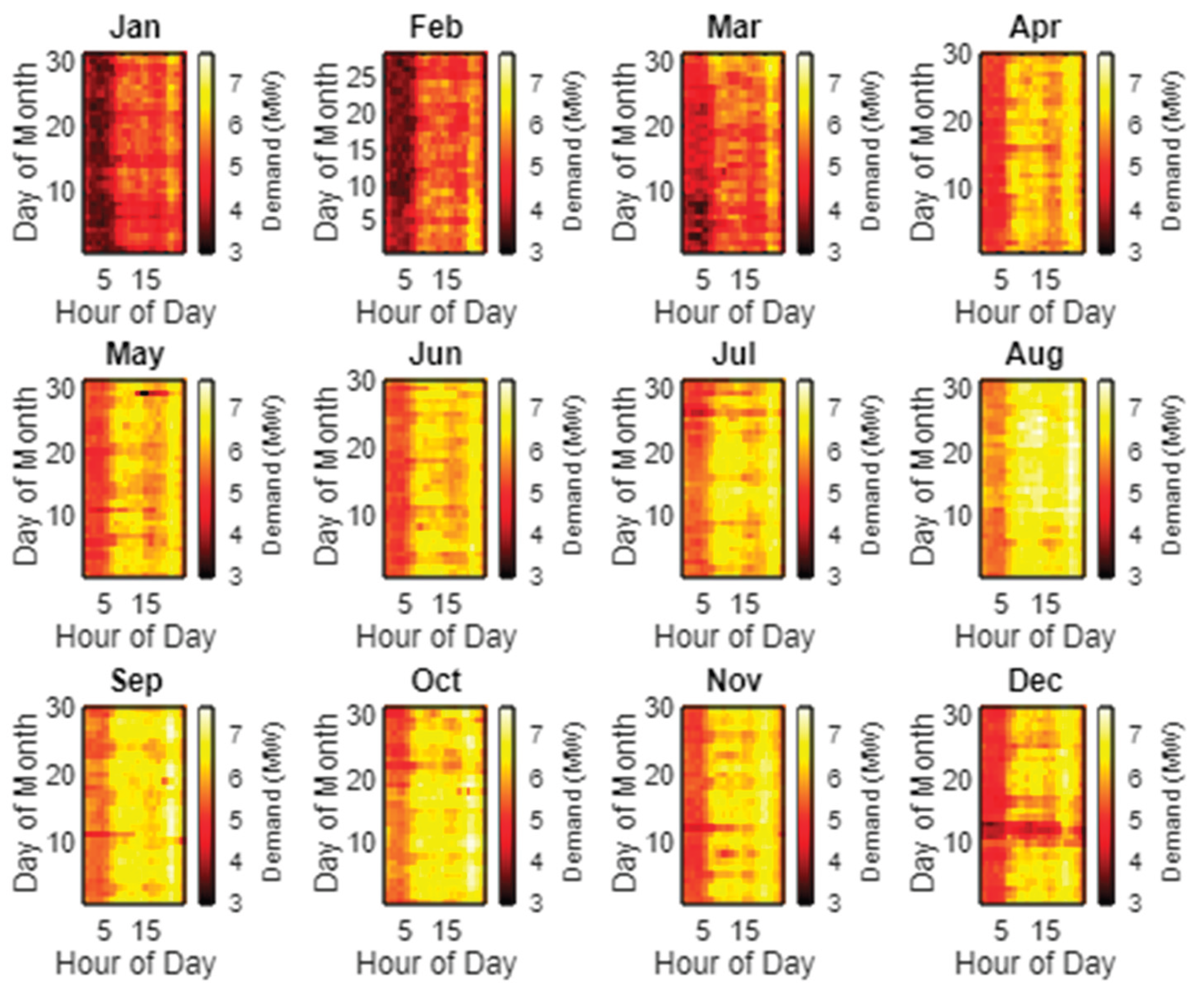
Figure 3.
Electricity demand profiles of the El Hierro Island: a) Hourly profiles for typical season days (year 2023); b) Monthly variability (obtained based on hourly data from 2014 to 2024 [32]).
Figure 3.
Electricity demand profiles of the El Hierro Island: a) Hourly profiles for typical season days (year 2023); b) Monthly variability (obtained based on hourly data from 2014 to 2024 [32]).
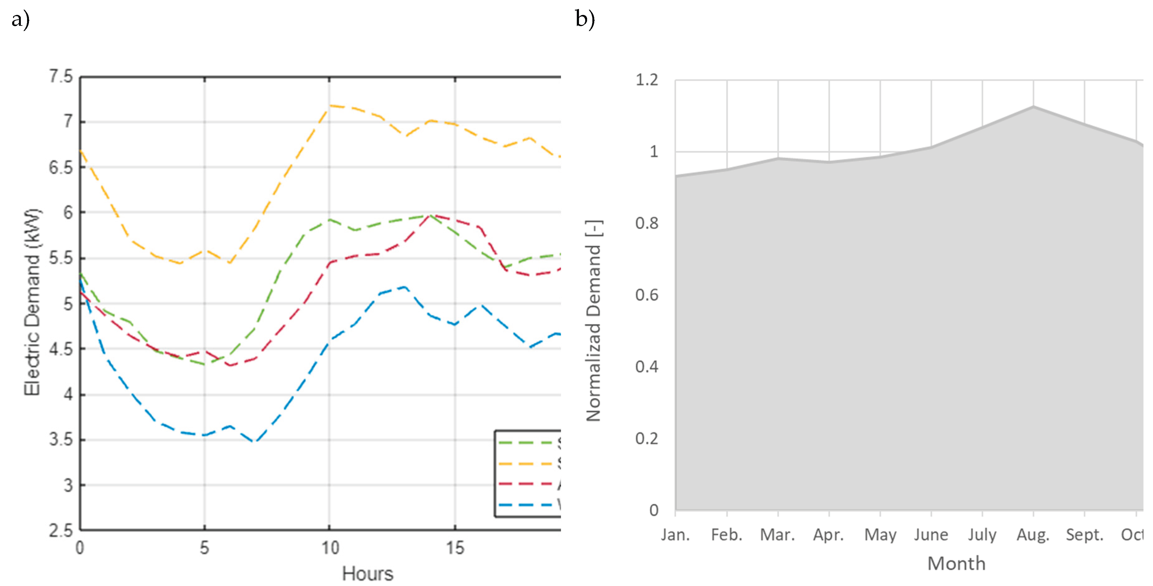
Figure 4.
Electric Power generation in the El Hierro island: a) Historical evolution; b) Breakdown of contributions over the last decade.
Figure 4.
Electric Power generation in the El Hierro island: a) Historical evolution; b) Breakdown of contributions over the last decade.
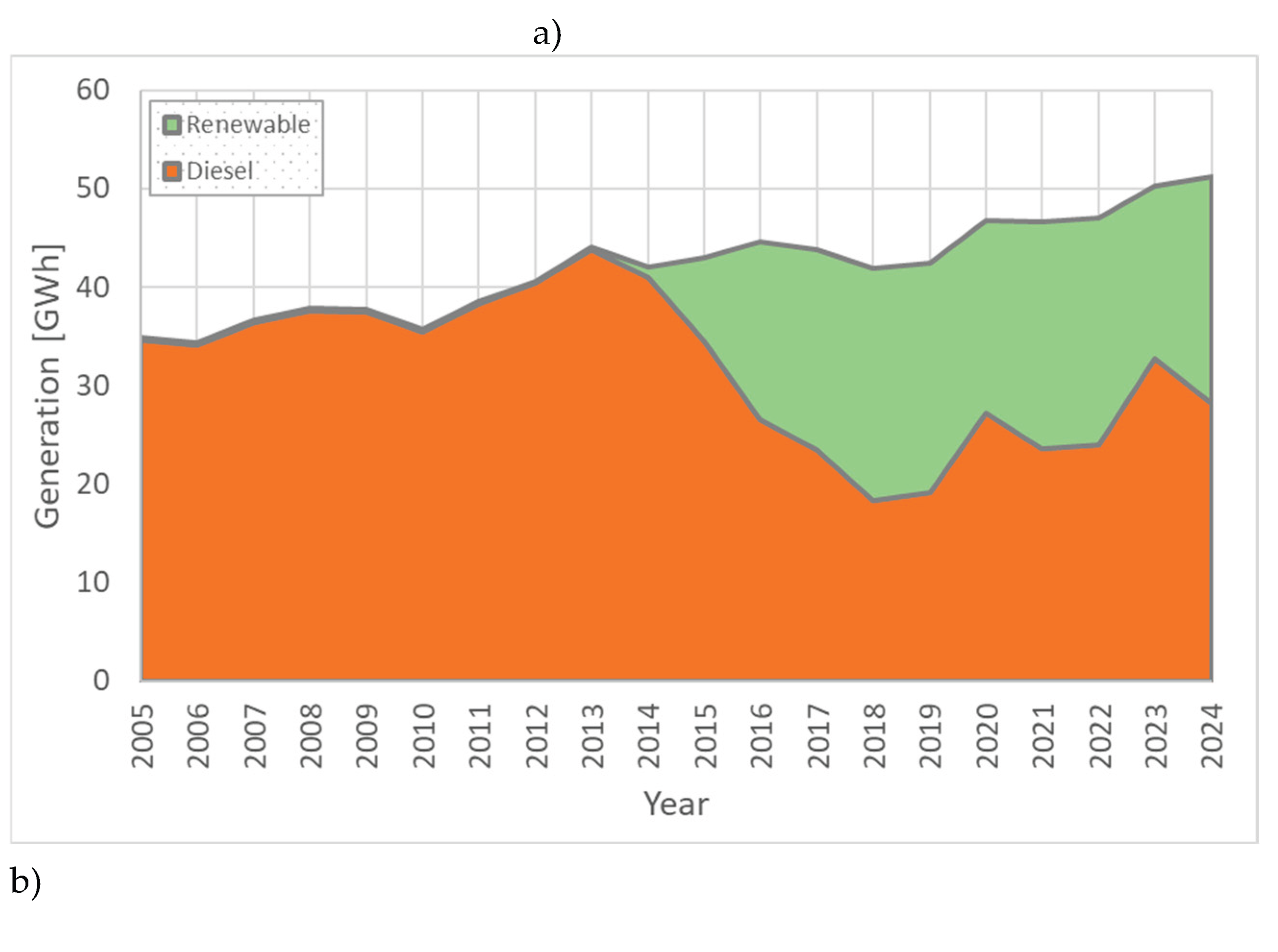
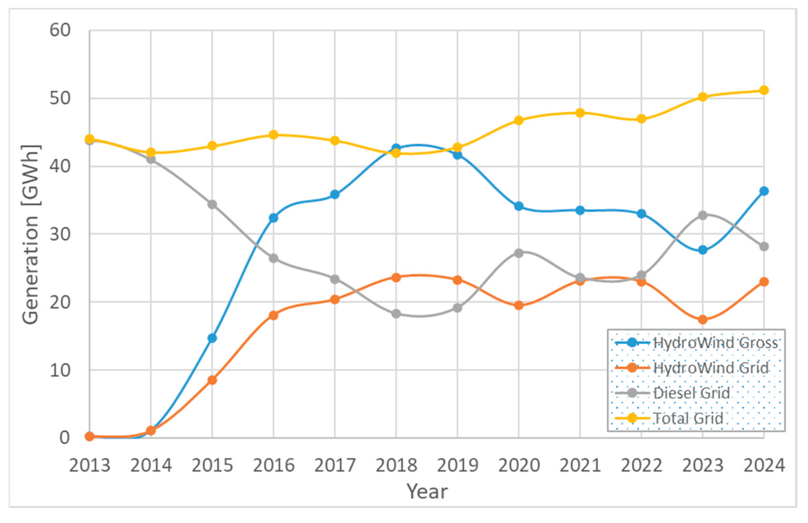
Figure 5.
Forecasts of the normalized values for the hourly EV charging profile in the El Hierro Island(data based on [47,49]).
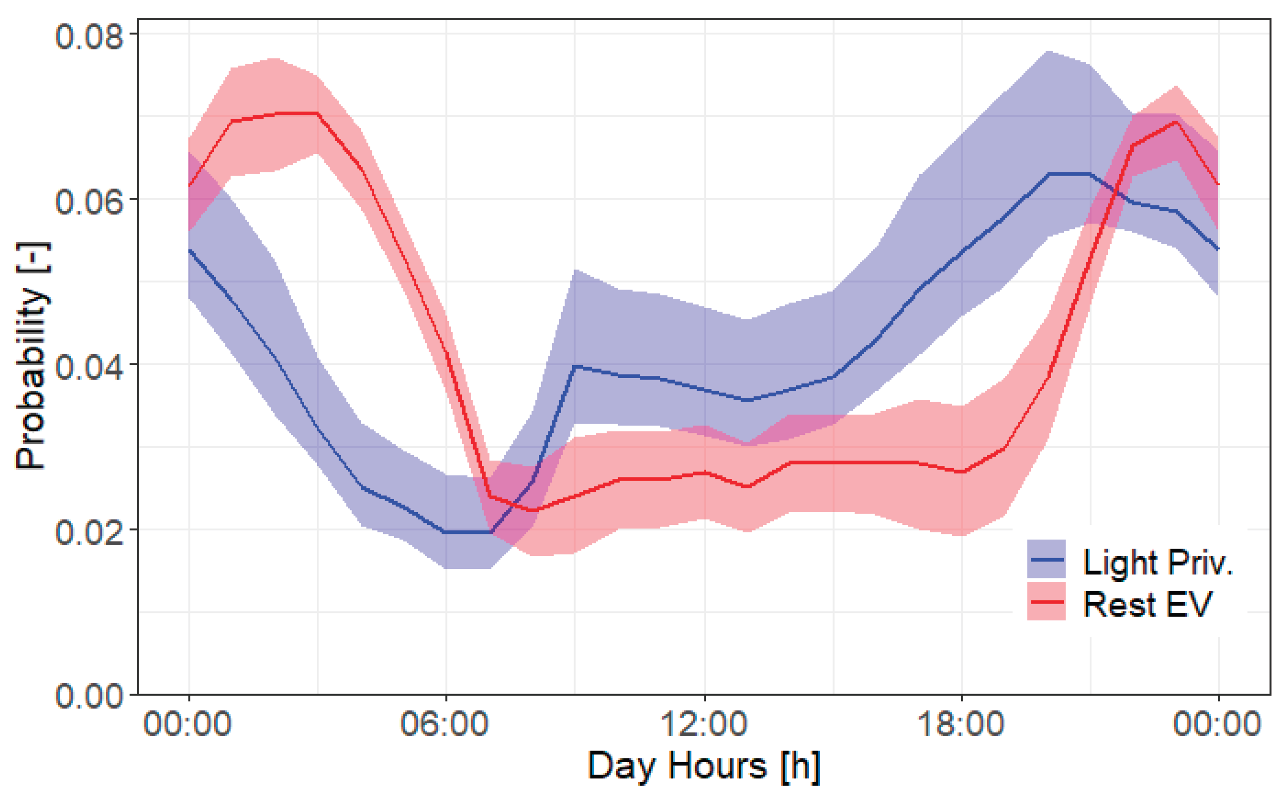
Figure 6.
Monthly seasonality associated with the traffic in Spain for 2021.
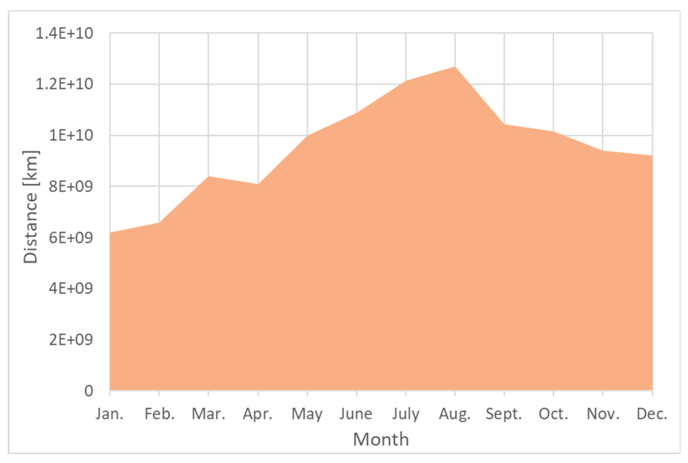
Figure 7.
Forecasted profiles of electric demand for the El Hierro Island by 2040, samples of typical: a) Winter Day (1st January); b) Summer Day (1st August).
Figure 7.
Forecasted profiles of electric demand for the El Hierro Island by 2040, samples of typical: a) Winter Day (1st January); b) Summer Day (1st August).
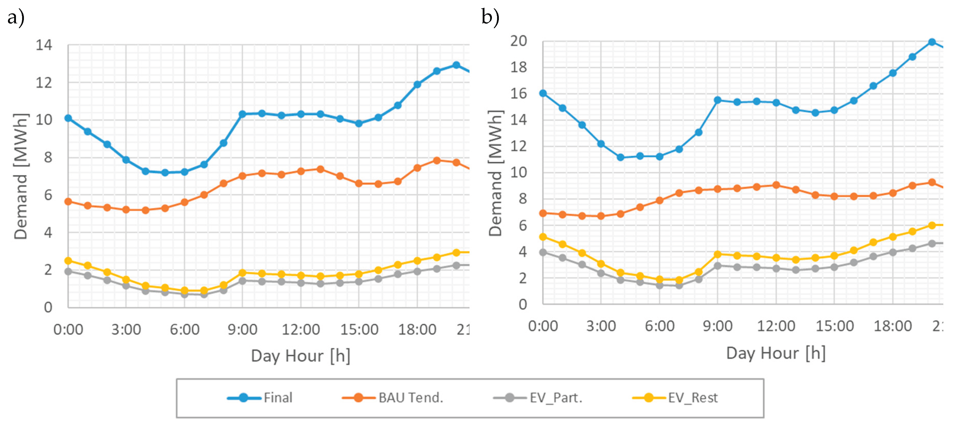
Figure 8.
Schematic overview with the essential input and output information of the HOMER software.
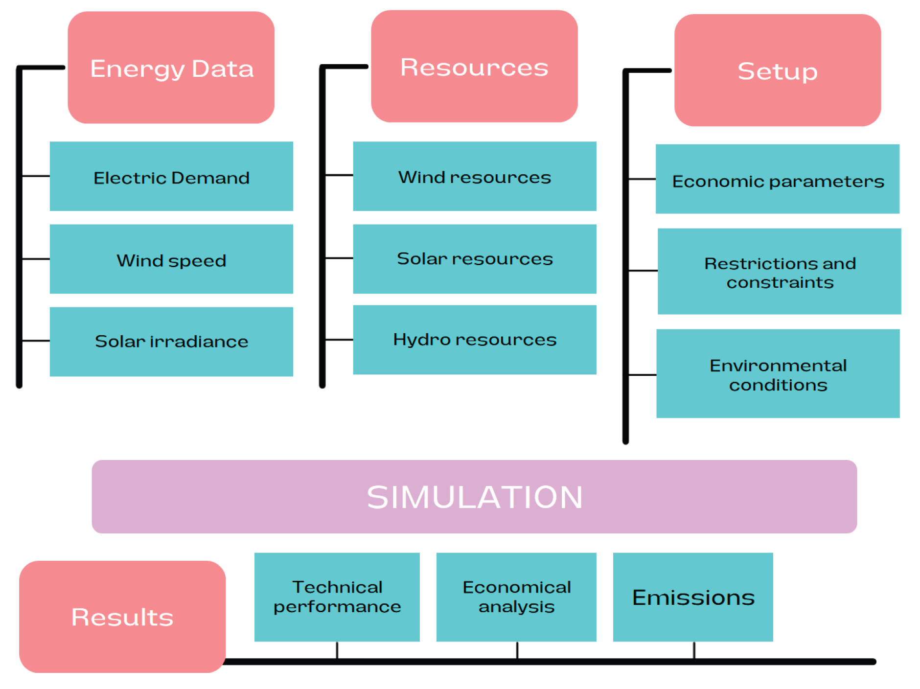
Figure 9.
Hourly demand curves for a typical day in the BAU scenario using the BEPU methodology: a) winter, b) summer.
Figure 9.
Hourly demand curves for a typical day in the BAU scenario using the BEPU methodology: a) winter, b) summer.
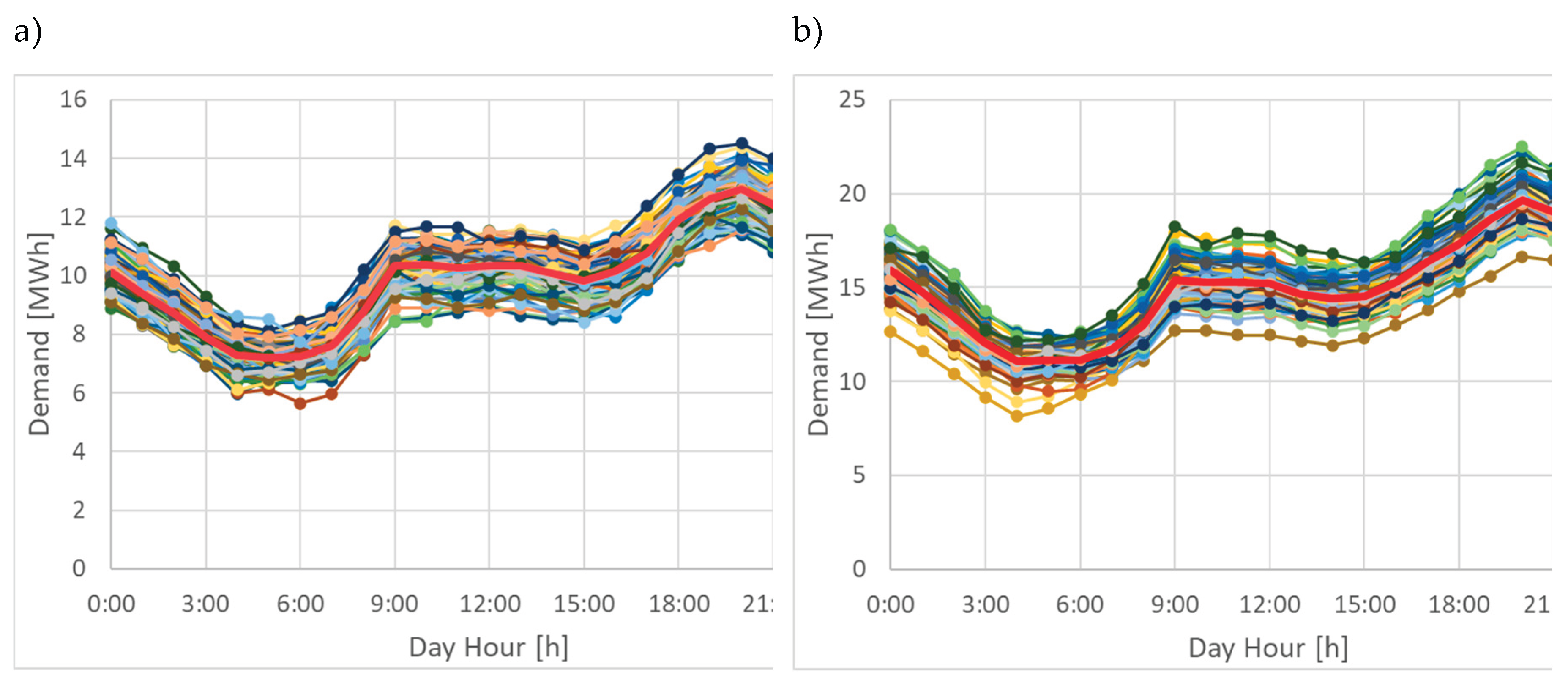
Figure 10.
Synthetic hourly profiles of solar irradiance for a typical day using the BEPU methodology: a) winter, b) summer.
Figure 10.
Synthetic hourly profiles of solar irradiance for a typical day using the BEPU methodology: a) winter, b) summer.
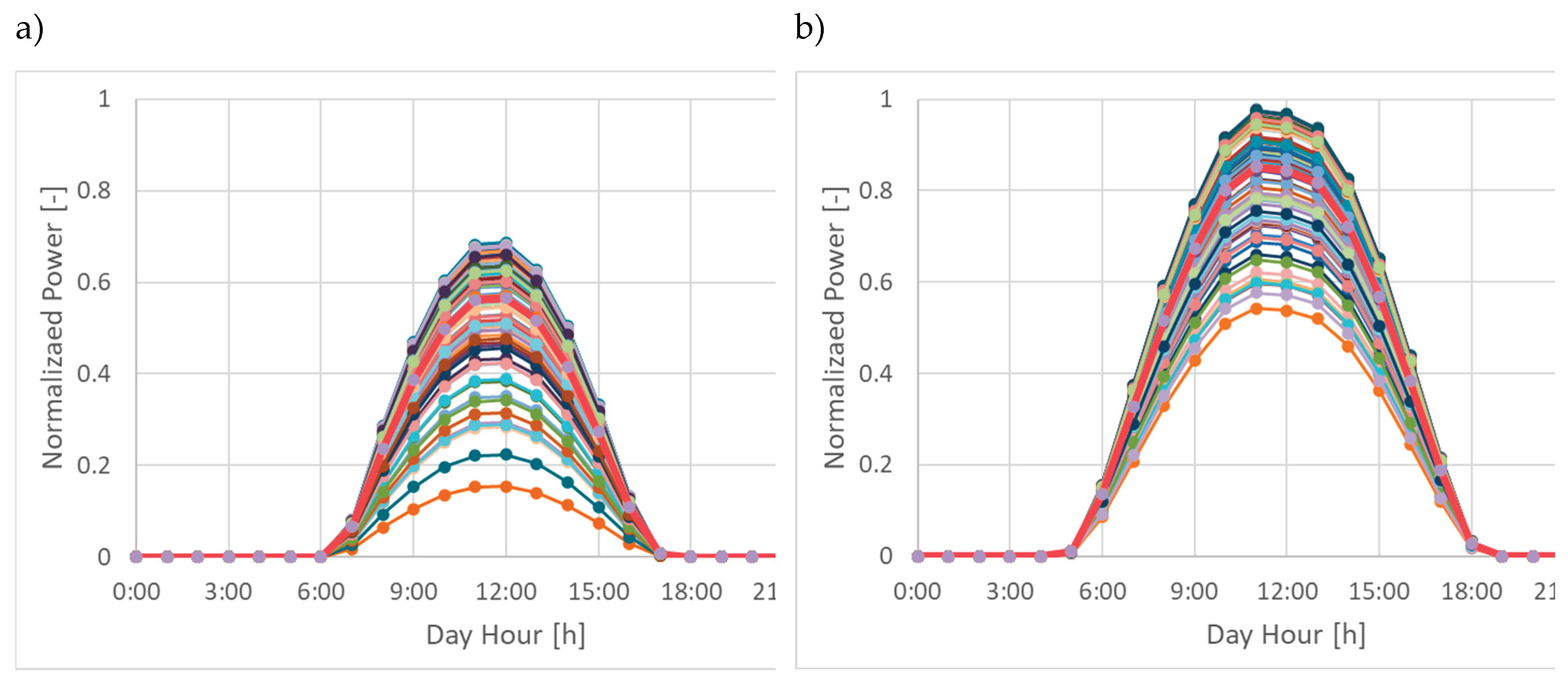
Figure 11.
Synthetic hourly wind profiles for a typical day using the BEPU methodology: a) winter, b) summer.
Figure 11.
Synthetic hourly wind profiles for a typical day using the BEPU methodology: a) winter, b) summer.
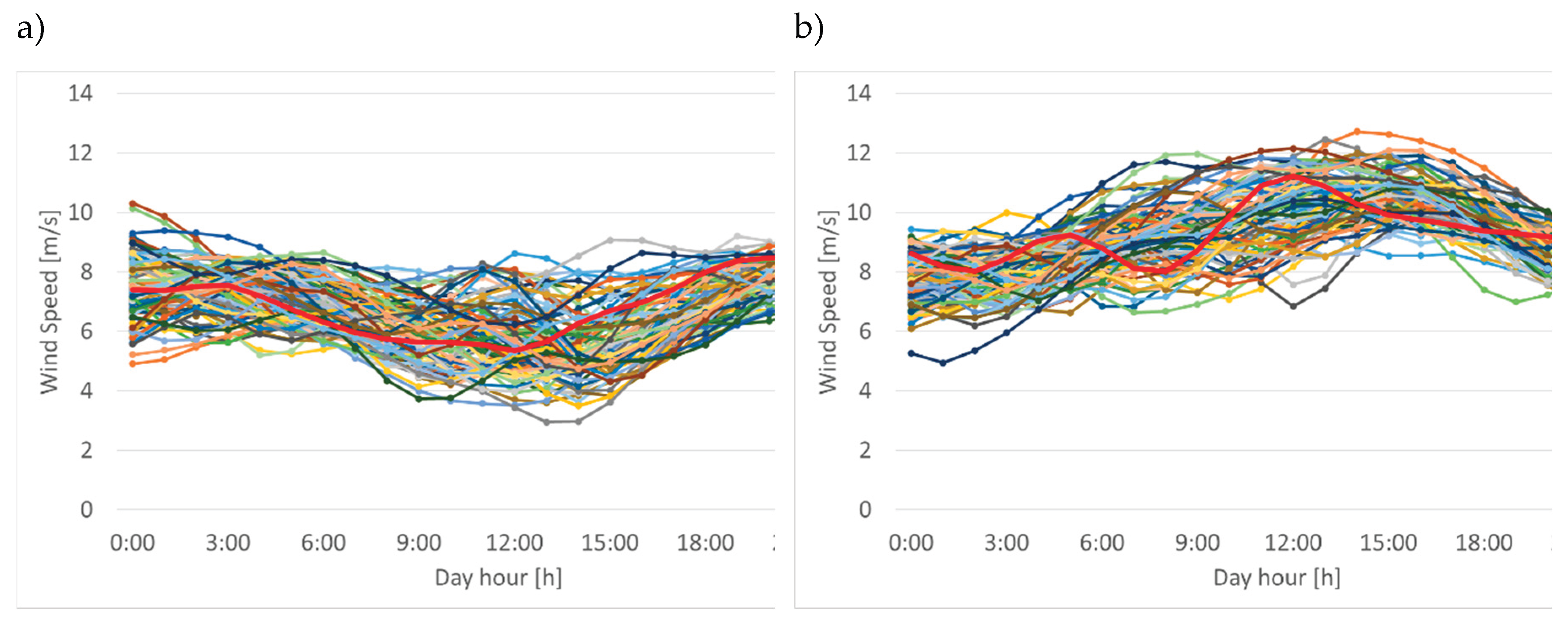
Figure 15.
Hourly performance of an averaged year for the reverse pumping system: a) Pumping; b) Turbination; c) Storage Capacity Percentage.
Figure 15.
Hourly performance of an averaged year for the reverse pumping system: a) Pumping; b) Turbination; c) Storage Capacity Percentage.
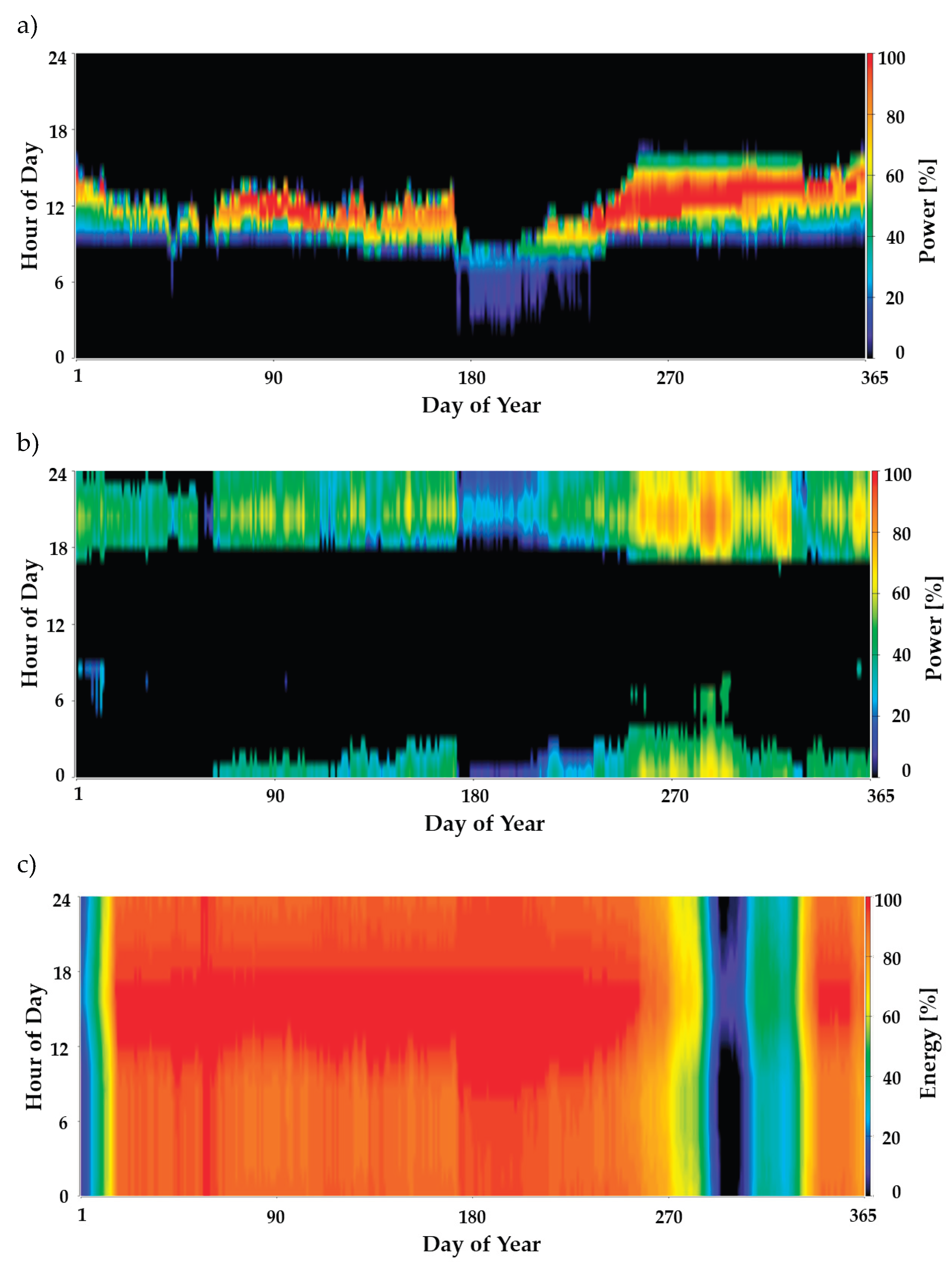
Figure 16.
Hourly performance of an averaged year for the mega-battery system: a) Charge; b) Discharge; c) State of Charge.
Figure 16.
Hourly performance of an averaged year for the mega-battery system: a) Charge; b) Discharge; c) State of Charge.
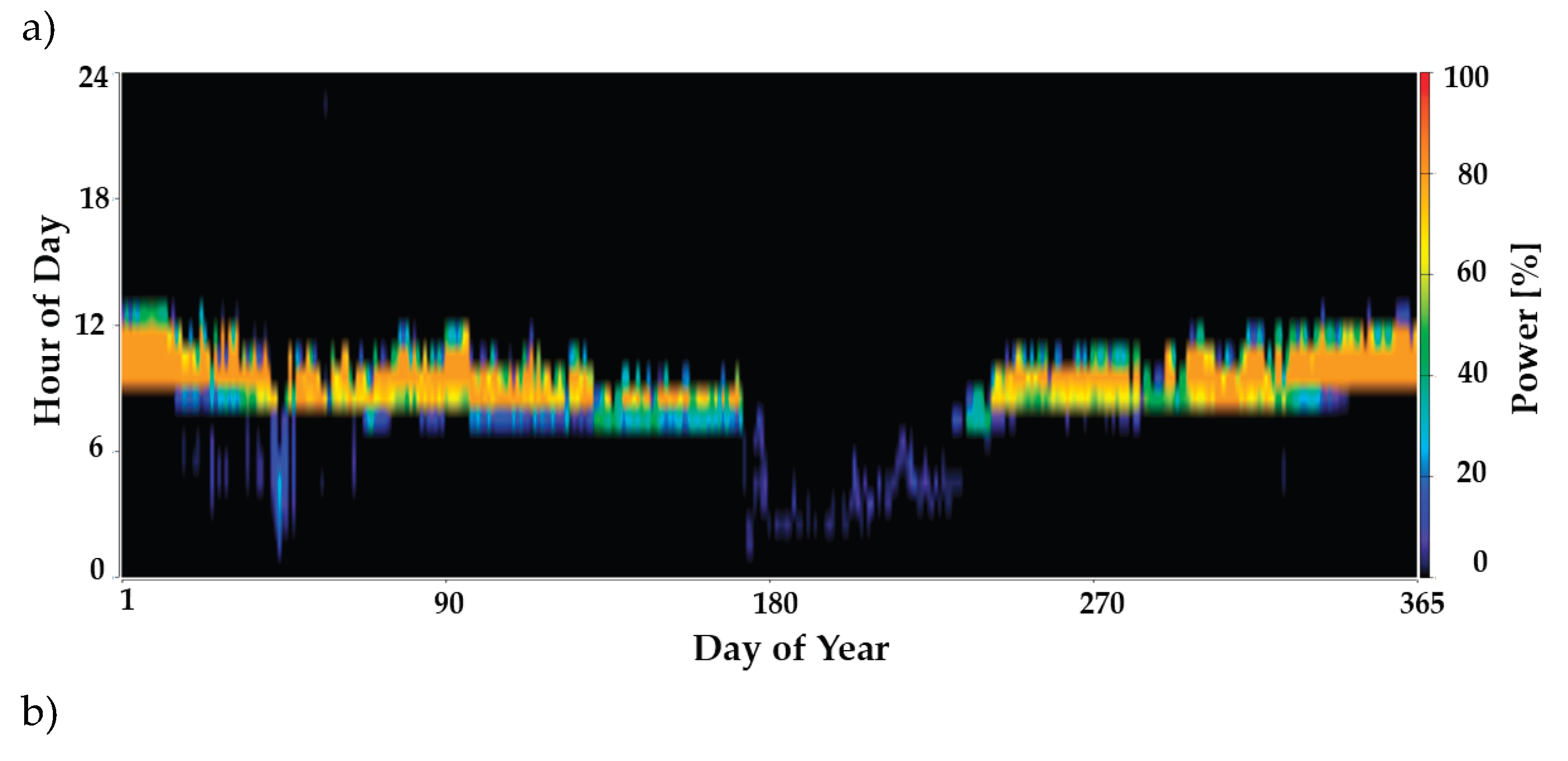
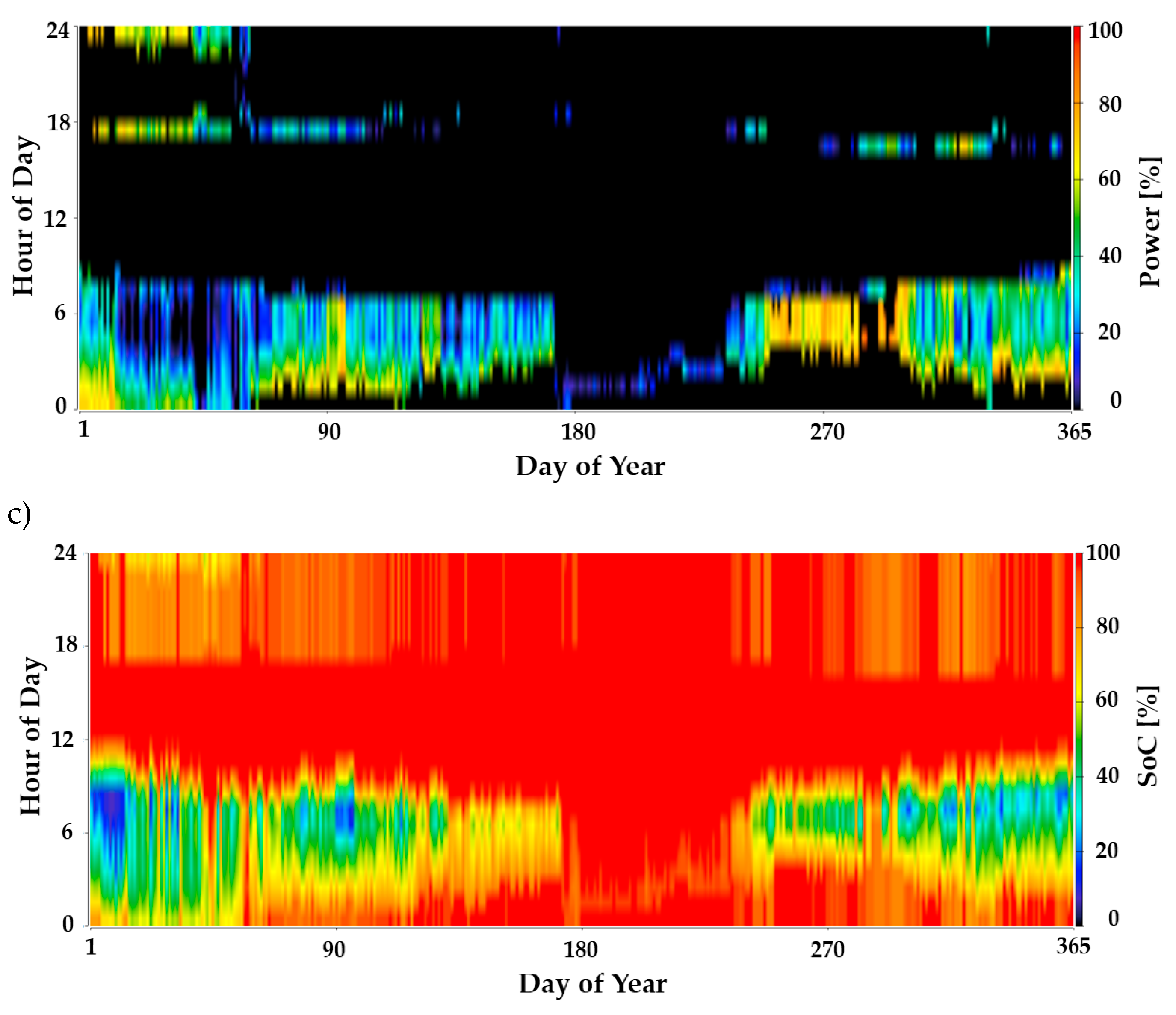
Figure 17.
Hourly diagram of the surpluses of the electric system over a complete year.
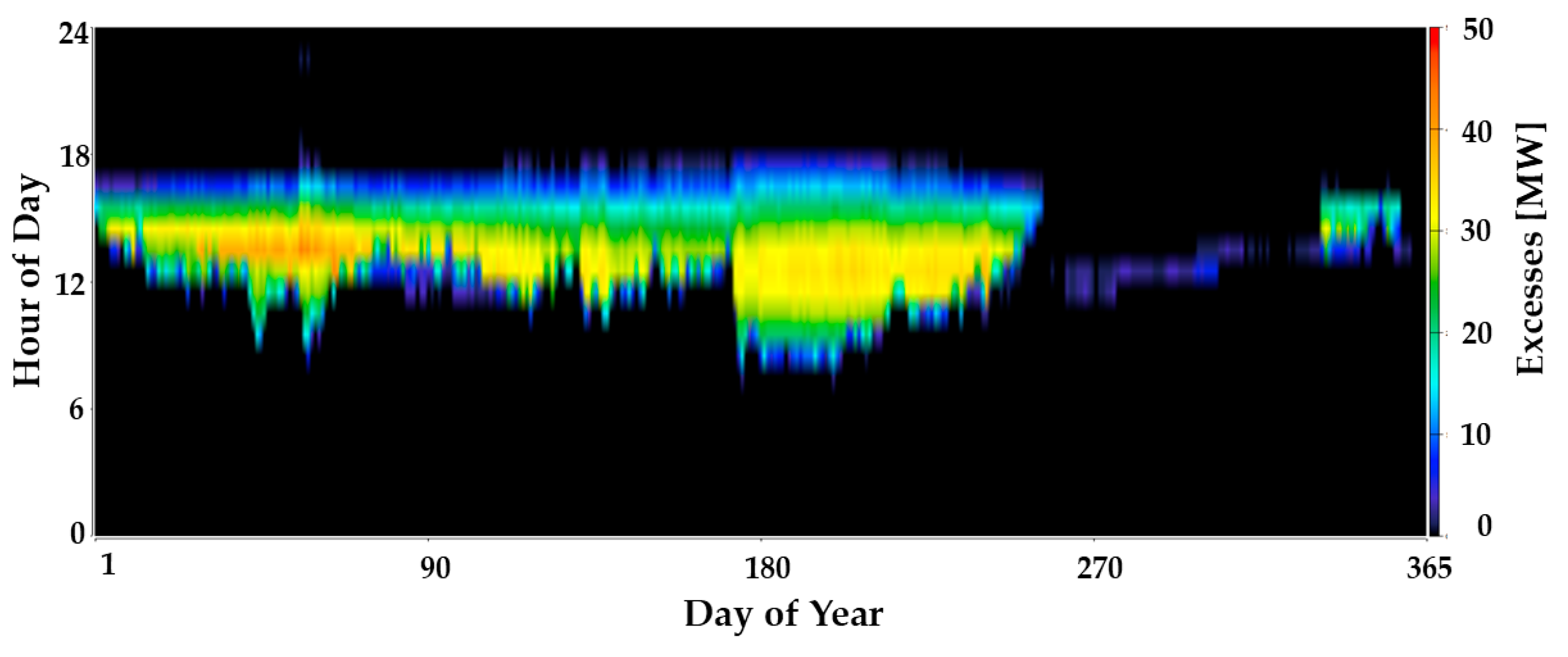
Figure 18.
Relation between unmet demand and generation surpluses for the 93 random sampling cases of the BAU scenario.
Figure 18.
Relation between unmet demand and generation surpluses for the 93 random sampling cases of the BAU scenario.
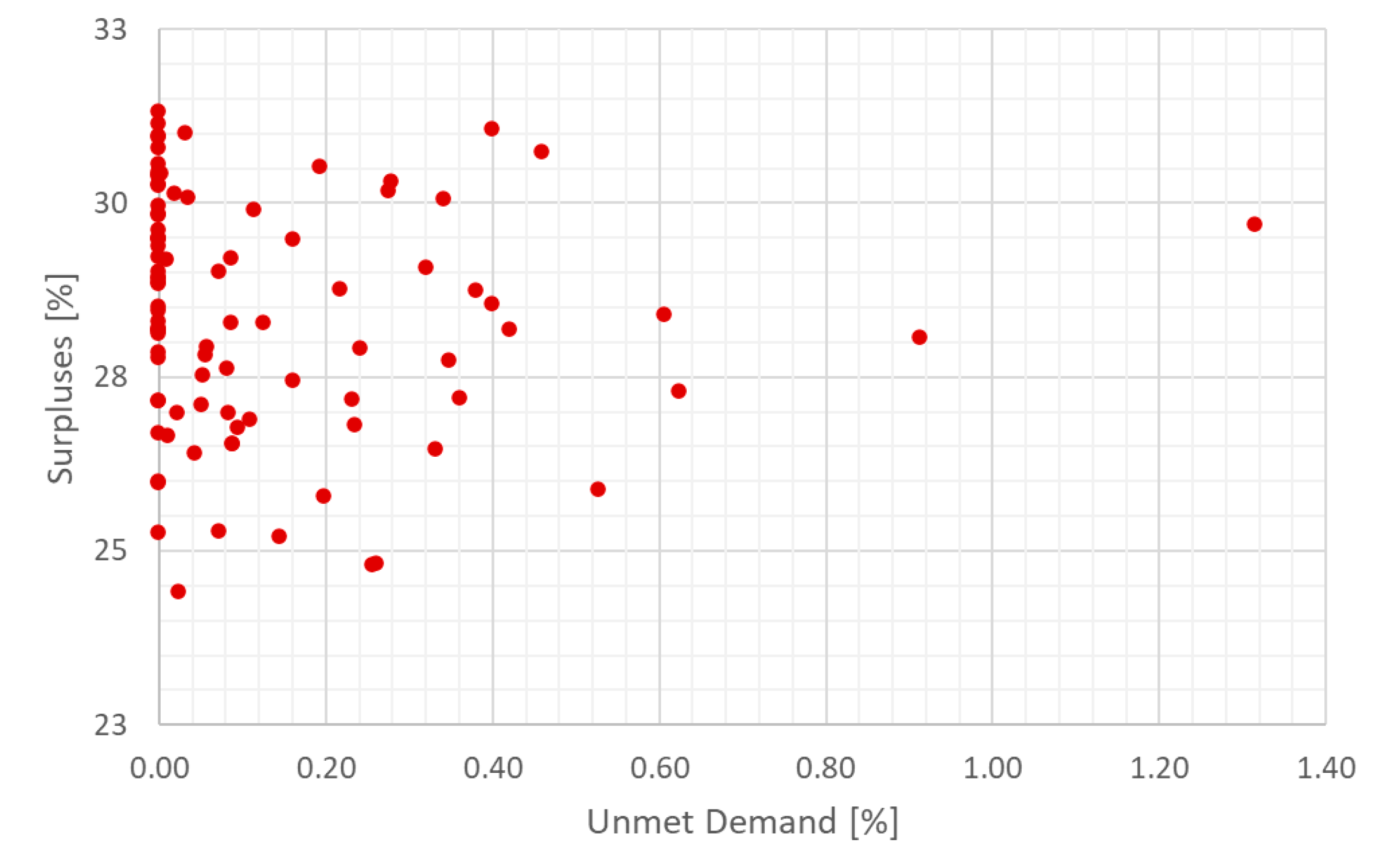
Figure 19.
Hourly demand curves for a typical day in the Efficiency scenario using the BEPU methodology: a) winter, b) summer.
Figure 19.
Hourly demand curves for a typical day in the Efficiency scenario using the BEPU methodology: a) winter, b) summer.
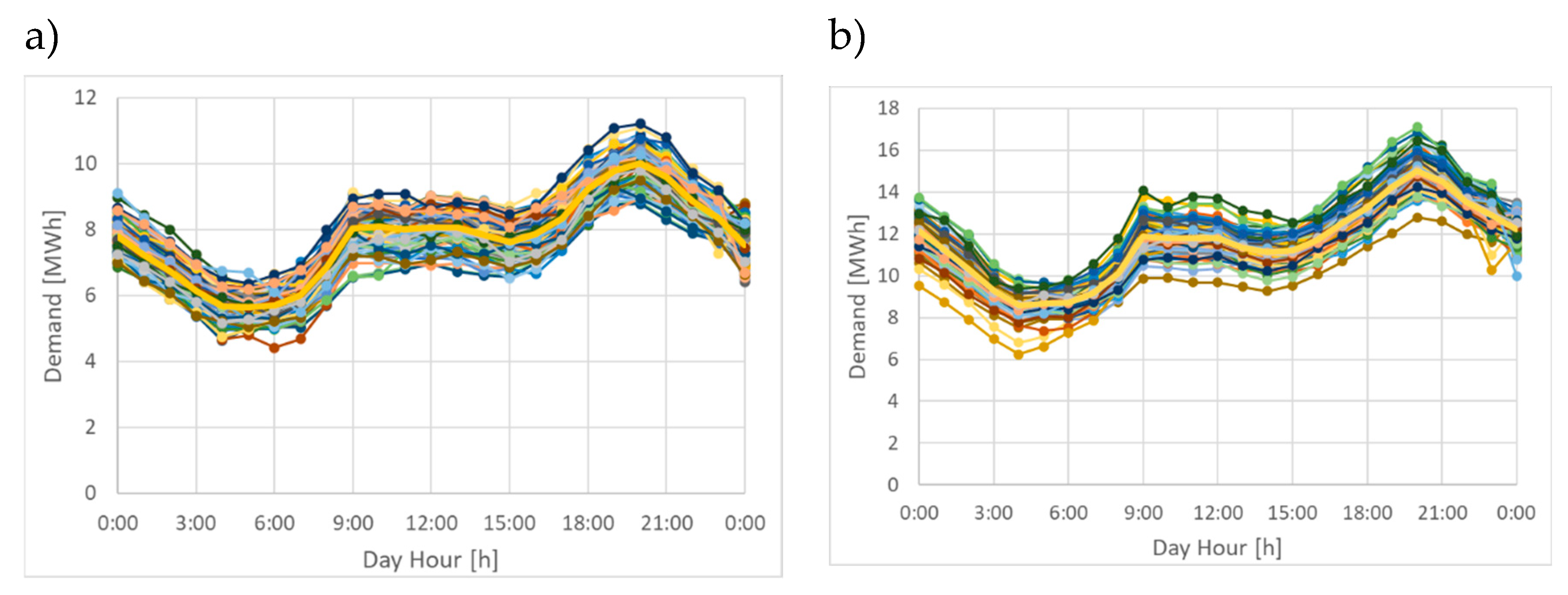
Figure 20.
Monthly performance of an averaged year for the storage systems: a) Reverse Pumping; b) Mega-battery.
Figure 20.
Monthly performance of an averaged year for the storage systems: a) Reverse Pumping; b) Mega-battery.
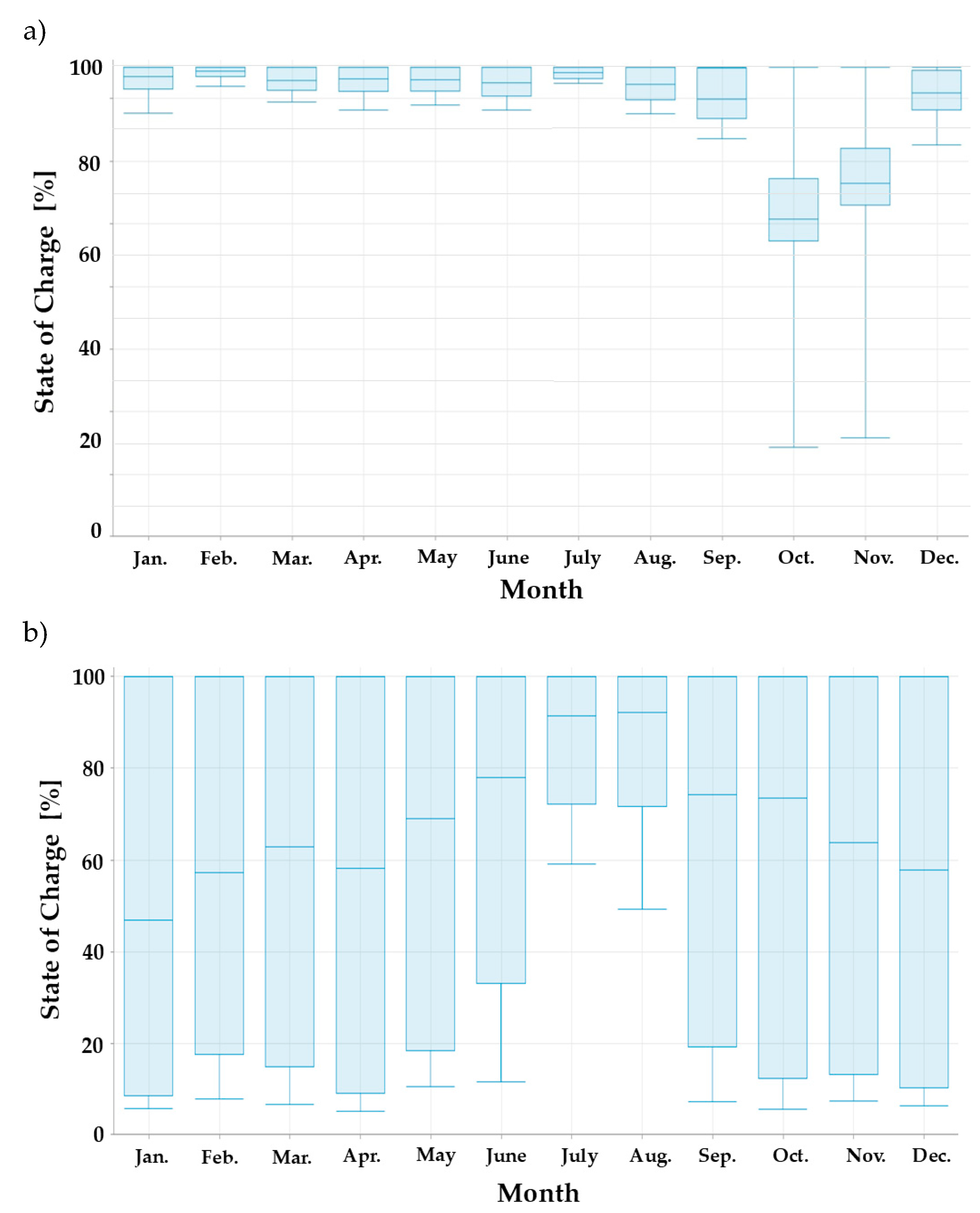
Figure 21.
Relation between unmet demand and generation surpluses for the 93 random sampling cases of the Efficiency scenario.
Figure 21.
Relation between unmet demand and generation surpluses for the 93 random sampling cases of the Efficiency scenario.
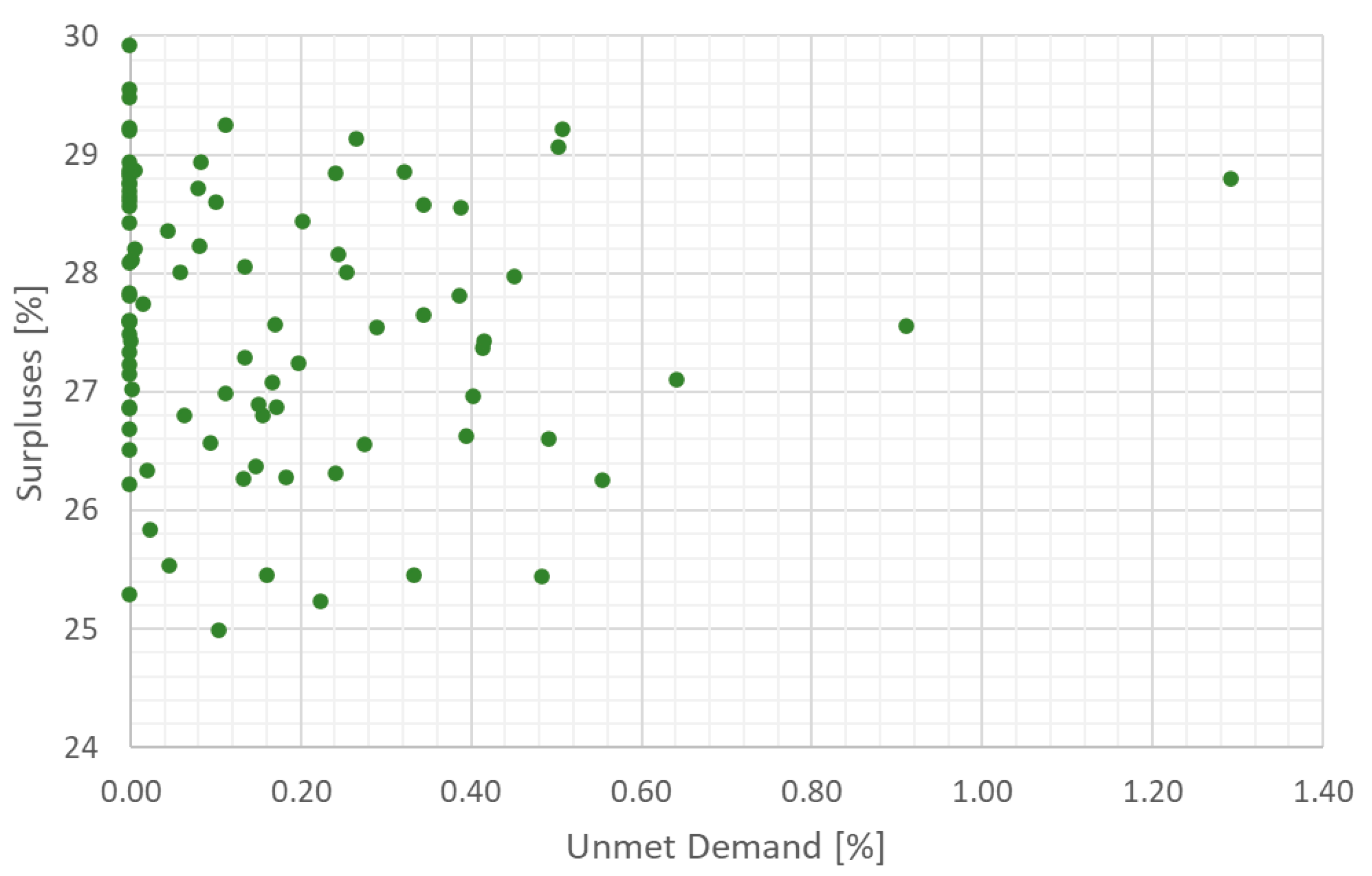
Table 1.
Summary of the EV Fleet Characteristics assuming 100% electrification and the conservative tendency (based on [47,48]).
| Vehicle type | Number of Vehicles | Consumption (kWh/km) |
Average Distance (km/day) |
Charge/Discharge Power | Capacity | Yearly Consumption (GWh) |
||
|---|---|---|---|---|---|---|---|---|
| Unitary (kW) | Total (MW) | Unitary (kWh) | Total (MWh) | |||||
| Car | 5618 | 0.15 | 50 | 3.7 | 20.79 | 80 | 449.4 | 18.49 |
| Motorcycle | 802 | 0.06 | 20 | 3.7 | 2.967 | 20 | 16.04 | 0.373 |
| Van | 1627 | 0.18 | 60 | 3.7 | 6.02 | 100 | 162.7 | 6.425 |
| Bus | 47 | 0.95 | 300 | 50 | 2.35 | 250 | 11.75 | 4.913 |
| Truck | 1885 | 0.64 | 30 | 50 | 94.25 | 300 | 565.5 | 13.14 |
| Wind generator | Enercon E-70 E4 |
| Rated power (MW) | 2.30 |
| Rotor diameter (m) | 71 |
| Height to the hub (m) | 98 m |
| Total height (m) | 133.5 m |
| Cut in wind speed | 2.5 m/s |
| Cur out wind speed | 34 m/s |
| Lifetime (years) | 25 |
| Cost of the system (M€/turbine) | 2.30 |
| M€/MW | 1.00 |
| O&M cost (M€/year) | 0.19 |
Table 3.
Inputs used for the PV system. [54]
Table 3.
Inputs used for the PV system. [54]
| Lifetime (years) | 25 |
| Derating factor (%) | 80 |
| Tracking system | No tracking |
| Solar panel | Vertex 550+ |
| Temperature coefficient of power (%/°C) | -0.38 |
| Peak Power (W) | 550 |
| Nominal operating cell temperature (°C) | 45 |
| Efficiency of the panel at standard conditions (%) | 21.1 |
| Cost (€/kW) | 900 |
| O&M cost (€/kW·year) | 13.5 |
Table 4.
Standard system specifications of the selected battery system Tesla Megapack 2XL. [57]
Table 4.
Standard system specifications of the selected battery system Tesla Megapack 2XL. [57]
| Maximum AC power (kW) | 979 |
| Energy available (MWh) | 3.916 |
| Round-trip system Efficiency (%) | 93.7 |
| Cost of the module (€) | 460,000 |
| O&M cost (€/year) | 5300 |
| Lifetime (years) | 25 |
Table 5.
Summary of the installed generation power, storage power and capacity, and energy production of the BAU scenario.
Table 5.
Summary of the installed generation power, storage power and capacity, and energy production of the BAU scenario.
| Generation Systems | |||||||
| Technology | Power (MW) | Energy | Surpluses | ||||
| GWh | % | GWh | % | ||||
| Solar PV | 53.0 | 90.96 | 58.45 | ----- | ----- | ||
| Wind | 16.1 | 64.66 | 31.55 | ----- | ----- | ||
| Total | 69.1 | 155.62 | 100 | 42.47 | 27.29 | ||
| Storage Systems | |||||||
| Technology |
Power In /Out (MW)1 |
Stored Energy (MWh) |
Energy In | Efficiency (%) | |||
| MWh | %2 | ||||||
| Hydro-Pump | 32 | 16 | 750 | 27.20 | 17.48 | 81 | |
| Batteries | 9.79 | 9.79 | 39.16 | 3.471 | 2.23 | 93.7 | |
| Total | 41.79 | 25.79 | 789.16 | 30.20 | 19.71 | ----- | |
1 Power In/Out refers to the Pumping/Turbination and Charge/Discharge processes for the reverse pumping and batteries, respectively; 2 percentage of energy recovered by the storage systems as a percentage of the total generated energy.
Table 6.
Capital, replacement, O&M, and total discounted costs for the sub-systems of the scenario..
Table 6.
Capital, replacement, O&M, and total discounted costs for the sub-systems of the scenario..
| Sub-Systems | Capital (M€) | Replacement (M€) | O&M (M€)1 | Total (M€)1 |
|---|---|---|---|---|
| PV | 48.7 | 38.19 | 15.58 | 101.5 |
| Wind | 16.1 | 12.88 | 8.41 | 37.4 |
| Reverse Pumping | 73.95 | 0 | 17.95 | 90.9 |
| Mega-Batteries | 4.6 | 7.35 | 1.154 | 13.1 |
| TOTAL | 141.9 | 58.4 | 43.1 | 242.9 |
1 Total costs over the 50-year life of the project.
Table 7.
Performance of the optimized deterministic system over a stochastic approach for the BAU scenario.
Table 7.
Performance of the optimized deterministic system over a stochastic approach for the BAU scenario.
| Base Case | Unfavourable Case | Favourable Case | |
|---|---|---|---|
| Renewable sources | |||
| Solar PV (GWh) | 90.96 | 90.65 | 91.86 |
| Wind (GWh) | 64.66 | 68.37 | 71.62 |
| Total (GWh) | 155.62 | 159.02 | 163.48 |
| Storage systems | |||
| Hydro pump (GWh) | 24.33 | 25.02 | 24.93 |
| Battery (GWh) | 3.471 | 3.403 | 4.696 |
| Total (GWh) | 27.80 | 28.42 | 29.63 |
| System Excesses/Unmet Demand | |||
| Generation Surpluses (GWh) | 42.47 | 47.31 | 50.61 |
| (%) | 27.29 | 29.70 | 30.94 |
| Unmet Demand (GWh) | 0 | 1.407 | 0 |
| (%) | 0 | 1.29 | 0 |
Table 8.
Performance of possible resized systems in the stochastic approach for the two extreme cases in the BAU scenario
Table 8.
Performance of possible resized systems in the stochastic approach for the two extreme cases in the BAU scenario
| Resized Solar PV | Resized Wind | Resized Batteries | Resized Solar PV/Batteries | ||||||
|---|---|---|---|---|---|---|---|---|---|
| Unfavour. Case | Favou. Case | Unfavour. Case | Unfavour. Case | Unfavour. Case | Favour. Case | Unfavour. Case | Favour. Case | ||
| Demand (GWh/year) | 108.43 | 108-07 | 108.43 | 108-07 | 108.43 | 108-07 | 108.43 | 108-07 | |
| Resizing (MW) | 14 MW PV Pannels | 6 Wind Turbines (13.8 MW) | 21 Batt (20.56MW, 82.24MWh) | 7 MW PV / 6 Batt (5.874MW, 23.50MWh) | |||||
| Generation (GWh) | 183.35 | 187.59 | 217.92 | 225.82 | 159.02 | 163.48 | 171.3 | 175.59 | |
| Generation Surpluses (GWh) | 63.39 | 68.94 | 101.87 | 111.23 | 45.37 | 52.71 | 55.59 | 61.09 | |
| (%) | 34.57 | 36.75 | 43.50 | 49.26 | 28.53 | 32.20 | 32.45 | 34.79 | |
| System Costs (M€) | 269.50 | 269.05 | 271.84 | 271.40 | 263.51 | 263.22 | 260.15 | 259.84 | |
| LCOE (c€/kWh) | 11.42 | 11.43 | 11.51 | 11.53 | 11.17 | 11.19 | 11.02 | 11.04 | |
Table 9.
Summary of the installed generation power, storage power and capacity, and energy production of the Efficiency scenario.
Table 9.
Summary of the installed generation power, storage power and capacity, and energy production of the Efficiency scenario.
| Generation Systems | |||||||
| Technology | Power (MW) | Energy | Surpluses | ||||
| GWh | % | GWh | % | ||||
| Solar PV | 42.0 | 72.08 | 60.95 | ----- | ----- | ||
| Wind | 11.5 | 46.19 | 39.05 | ----- | ----- | ||
| Total | 53.5 | 118.27 | 100 | 31.26 | 26.43 | ||
| Storage Systems | |||||||
| Technology |
Power In /Out (MW)1 |
Stored Energy (MWh) |
Energy In | Efficiency (%) | |||
| MWh | %2 | ||||||
| Hydro-Pump | 25 | 12 | 500 | 17.08 | 14.44 | 81 | |
| Batteries | 9.79 | 9.79 | 39.16 | 5.97 | 5.05 | 93.7 | |
| Total | 34.79 | 21.79 | 539.16 | 23.51 | 19.49 | ----- | |
Table 10.
Capital, replacement, O&M, and total discounted costs for the sub-systems of the Efficiency scenario.
Table 10.
Capital, replacement, O&M, and total discounted costs for the sub-systems of the Efficiency scenario.
| Sub-Systems | Capital (M€) | Replacement (M€) | O&M (M€)1 | Total (M€)1 |
|---|---|---|---|---|
| PV | 37.8 | 30.26 | 12.35 | 80.4 |
| Wind | 15.5 | 9.20 | 6.01 | 26.7 |
| Reverse Pumping | 54.75 | 0 | 12.21 | 67.0 |
| Mega-Batteries | 4.6 | 7.35 | 1.154 | 13.1 |
| TOTAL | 108.7 | 46.8 | 31.7 | 186.6 |
1 Total costs over the 50-year life of the project.
Table 11.
Performance of the optimized deterministic system over a stochastic approach for the Efficiency scenario.
Table 11.
Performance of the optimized deterministic system over a stochastic approach for the Efficiency scenario.
| Base Case | Unfavourable Case | Favourable Case | |
|---|---|---|---|
| Renewable sources | |||
| Solar PV (GWh) | 72.08 | 71.62 | 72..86 |
| Wind (GWh) | 46.19 | 49.29 | 51.09 |
| Total (GWh) | 118.27 | 120.91 | 123.95 |
| Storage systems | |||
| Hydro pump (GWh) | 17.08 | 16.40 | 13.29 |
| Battery (GWh) | 5.97 | 7.27 | 6.53 |
| Total (GWh) | 23.15 | 23.67 | 19.82 |
| System Excesses/Unmet Demand | |||
| Generation Surpluses (GWh) | 8.35 | 13.11 | 15.29 |
| (%) | 7.06 | 10.84 | 12.33 |
| Unmet Demand (GWh) | 0 | 1.067 | 0 |
| (%) | 0 | 1.29 | 0 |
Disclaimer/Publisher’s Note: The statements, opinions and data contained in all publications are solely those of the individual author(s) and contributor(s) and not of MDPI and/or the editor(s). MDPI and/or the editor(s) disclaim responsibility for any injury to people or property resulting from any ideas, methods, instructions or products referred to in the content. |
© 2025 by the authors. Licensee MDPI, Basel, Switzerland. This article is an open access article distributed under the terms and conditions of the Creative Commons Attribution (CC BY) license (http://creativecommons.org/licenses/by/4.0/).
Copyright: This open access article is published under a Creative Commons CC BY 4.0 license, which permit the free download, distribution, and reuse, provided that the author and preprint are cited in any reuse.


