
Submitted:
09 May 2025
Posted:
09 May 2025
You are already at the latest version
Abstract
Accurate estimation of uniaxial compressive strength (UCS) of carbonate rocks is critical for the design and stability assessment of geotechnical structures in karst‐influenced environments. This study evaluates four feed-forward artificial neural network (ANN) architectures as Radial Basis Function (RBF), Bayesian Regularized (BR), Scaled Conjugate Gradient (SCG), and Levenberg–Marquardt (LM) to predict UCS from three readily measured inputs: water content, interconnected porosity, and real density. A dataset of 50 core specimens from the Seybaplaya quarry in Campeche, Mexico, was partitioned into training and testing subsets under consistent preprocessing. Model performance was assessed via mean absolute error (MAE), root mean squared error (RMSE), mean absolute percentage error (MAPE), and coefficient of determination (R²), averaged over 30 independent runs. Statistical significance of differences in test-set mean squared error (MSE) was examined using the Friedman test with Benjamini–Hochberg correction. Sensitivity analysis based on partial derivatives quantified the relative influence of each input feature.The RBF network achieved the highest predictive accuracy (median R² = 0.975; RMSE = 1.313 MPa) and significantly outperformed BR and SCG models (adjusted p < 0.01). Bayesian regularization offered robust generalization (MAE = 1.164 MPa; R² = 0.967), while SCG and LM converged faster but with slightly lower accuracy. Sensitivity scores indicated interconnected porosity (54.4 %) as the dominant driver of UCS predictions, followed by water content (30.9 %) and real density (14.7 %). These findings demonstrate that RBF-based ANNs, combined with appropriate regularization and sensitivity assessment, provide a reliable framework for UCS prediction in heterogeneous carbonate formations.

Keywords:
uniaxial compressive strength
; carbonate rock cores
; artificial neural networks
; radial basis function
; Bayesian regularization
; sensitivity analysis
1. Introduction
Accurate prediction of uniaxial compressive strength (UCS) of rock masses is essential for the safe and cost-effective design of geotechnical and civil infrastructure. Traditional empirical and regression-based models, such as those relating UCS to porosity, density, or ultrasonic velocity offer useful first-order estimates but often fail when applied to heterogeneous, partially saturated, or karst-affected formations due to their reliance on assumed functional forms and minimal textural variability [1,2,3]. In complex carbonate environments like the Seybaplaya bank rocks of Campeche, Mexico, where mixed bioclastic limestones, coquinas, and breccias exhibit wide ranges of water content, porosity, and density. These limitations become particularly acute.
Recent advances in machine learning, and in particular artificial neural networks (ANNs), have demonstrated superior capability to capture nonlinear, multivariate interactions among geomechanical inputs without presupposing explicit correlation structures. By integrating metrics such as water content, interconnected porosity, and real density, ANNs have achieved higher predictive accuracy for UCS across diverse lithologies and saturation states [4,5]. Moreover, hybrid and optimized frameworks, ranging from ANFIS to PSO-tuned networks have further underscored the flexibility of data-driven approaches in rock mechanics engineering contexts.
Despite these successes, the comparative performance of different ANN training algorithms and regularization schemes remains underexplored for Seybaplaya formation rocks. Understanding how variations in network architecture, such as Radial Basis Function, Bayesian regularization, Scaled Conjugate Gradient, and Levenberg–Marquardt methods, affect convergence speed, generalization capacity, and robustness to measurement noise is critical for guiding practitioners in model selection and deployment.
Accordingly, this study implements and systematically evaluates four feed-forward ANN variants to predict UCS from water content, porosity, and density for 50 rock core specimens collected at the Seybaplaya quarry. Standardized preprocessing, consistent data splits, and uniform performance metrics (MAE, RMSE, MAPE, R²) enable transparent comparison. A Friedman statistical analysis and a partial-derivatives sensitivity assessment further illuminate the significance of algorithmic choice and the relative influence of each input variable on model outputs. Through this framework, we identify the optimal neural-network strategy for robust UCS estimation in karst-influenced carbonate settings.
2. Related Works
2.1. Empirical and Regression-Based Approaches
A considerable body of literature has explored empirical correlations between com-pressive strength and intrinsic rock properties [6,7]. For example, Peng and Zhang [8] evaluated sandstone, shale, limestone, and dolomite formations in the Gulf of Mexico, establishing linear, logarithmic, or exponential relationships. Their findings generally indicated that porosity negatively impacts uniaxial compressive strength (UCS), while density tends to correlate positively with rock strength. Nevertheless, such empirical models can perform poorly for heterogeneous materials or in situations where water saturation significantly modifies a rock’s mechanical response.
Freyburg [9] also proposed predictive equations for compressive strength based on ultrasonic velocity and porosity in various sedimentary rocks as sandstone and coal measures. Although such models offered valuable insights for more uniform lithologies, they frequently assume minimal mineralogical or textural variability. This assumption does not align well with the complex geology found in Seybaplaya, where mixed carbonate and clay minerals complicate the direct application of generic correlations.
2.2. Influence of Rock Properties on Compressive Strength
Several studies have highlighted how water content, porosity, and density individu-ally affect compressive strength [10,11]. Slight variations in water content can induce measurable changes in UCS, particularly in partially to fully saturated rock samples [12]. Elevated water content reduces effective cohesion and increases pore pressure, promoting microcrack propagation and weakening the rock matrix.
Porosity also plays a decisive role: higher porosity often correlates with lower UCS because it introduces additional voids and potential crack paths. At the same time, density, which is closely tied to porosity, generally reflects the rock’s load-bearing capacity [13]. Rocks of higher density tend to exhibit fewer voids, enhancing their mechanical strength [14]. However, as Lal [15] emphasized, porosity-related parameters must be contextualized within a rock’s mineralogy and textural characteristics. Consequently, direct correlations such as “UCS vs. porosity” or “UCS vs. density” may prove insufficient for karst-affected formations like those in Seybaplaya, where partial saturation and heterogeneous microstructures introduce significant scatter in measurements.
2.3. Neural Networks for Predictive Modeling in Geomechanics
While traditional regression-based methods remain common, they often struggle with capturing the highly nonlinear and multivariate interactions found in real-world geologic systems. This limitation has spurred a growing interest in machine learning (ML) approaches, particularly artificial neural networks (ANNs), which do not presume any specific functional form and are thus well-suited to modeling complex or hidden relationships [16]. By incorporating multiple input variables such as water content, porosity, density, and even sonic velocity, neural networks can learn to predict UCS more accurately than polynomial or linear regression in many cases [17].
For instance, Gokceoglu [5] showed that ANN models outperformed regression analyses for diverse rock types, leveraging petrographic and physical data to capture intricate variable interactions. Likewise, Galván and Restrepo [4] demonstrated that integrating moisture parameters into an ANN framework improved UCS predictions for calcareous and clastic rocks. These findings validate neural networks as a promising alternative for sites with significant lithological diversity, partial saturation, or karstic features, characteristic of Seybaplaya.
2.4. Empirical and Regression–Based Approaches
Wei et al [18] developed multilayer perceptron models to estimate UCS from dry density, Brazilian tensile strength, and saturated density in sedimentary rocks from the Thar coalfield, Pakistan. Their ANN model (70/30 training/test split) achieves R² up to 0.83 and outperforms multiple linear regression by a wide margin.
Torabi-Kaveh et al [19] apply both MLR and ANN (LM-trained MLP) to Asmari carbonate samples, demonstrating that ANN yields the lowest RMSE and highest R² for joint prediction of UCS and Young’s modulus. They highlight the decisive role of P-wave velocity and porosity in driving model accuracy.
Yagiz et al [20] compare nonlinear regression and LM-ANN models on Turkish travertine and limestone, incorporating Slake durability indices (Id2, Id4). Their results show that a four-cycle slake index (Id4) plus Schmidt hardness and P-wave velocity form an optimal predictor set, with ANN outperforming regression in R² and RMSE.
Setayeshirad et al [21] combine petrographic microfacies classification with MLR and LM-ANN on Ilam Formation carbonates. Their ANN achieves a highly parsimonious model (effective parameters <10) and R² > 0.91, illustrating the value of sensitivity-analysis-driven input selection.
Ceryan et al [22] employ Mallow’s Cp–based variable selection to identify total porosity and P-wave velocity as sufficient predictors of UCS in Kireçhane Formation limestones. Their LM-ANN model yields the lowest RMSE and highest R² compared to MLR, with Mann–Whitney U tests confirming the homogeneity of predicted versus measured distributions.
2.5. Neural Networks for Predictive Modeling in Geomechanics
Abdi and Taheri-Garavand [23] employed 130 sandstone specimens to develop an ANFIS model that estimates both uniaxial compressive strength (UCS) and elastic modulus (E) based on porosity, P-wave velocity, dry density, slake durability index (Id₂), and water absorption. Their optimized UCS predictor achieved an R² of 0.910, RMSE of 0.070, and VAF of 97%, whereas the (E) model yielded an R² of 0.866, RMSE of 0.086, and VAF of 89%.
Umrao et al. [24] compiled 45 measurements from sandstone, limestone, and shale samples sourced from the Umrer, Singrauli, and Kutch formations to train ANFIS models using density, porosity, and P-wave velocity as inputs. Their optimal UCS predictor achieved an R² of 0.935, RMSE of 4.69 MPa, and VAF of 95.6%, while the corresponding elastic modulus model reached an R² of 0.955, RMSE of 2.26 GPa, and VAF of 95.43%.
Cabalar et al. [25] present a comprehensive survey of ANFIS implementations across a range of geotechnical challenges, spanning UCS estimation, resonant-column shear modulus and damping, tunnel stability assessment, scour prediction, and foundation behavior analysis, and demonstrate that ANFIS consistently outperforms conventional regression methods in both accuracy and robustness.
Mohamad et al. [26] utilized 40 weathered shale specimens from Johor, Malaysia to develop a hybrid PSO-optimized ANN for UCS prediction, incorporating Brazilian tensile strength, point-load index, ultrasonic pulse velocity (Vp), and bulk density as inputs. Compared to a conventional back-propagation ANN, the PSO-ANN achieved superior performance, variance exceeding 95%, a lower RMSE, and a higher adjusted R², demonstrating its excellent predictive capability.
Momeni and Rashidi [27] evaluated 60 sandstone simples, measuring P-wave velocity, dry density, and Schmidt hardness, to train an MLP whose weights were optimized via PSO. Their best model achieved an R² of 0.974, RMSE of 0.086, and VAF of 97.5%, underscoring the efficacy of PSO-tuned ANNs for rapid UCS estimation.
Dehghan et al. [28] conducted 228 UCS tests on 38 Johor sandstone samples, using dry density, moisture content, P-wave velocity, point-load index, and slake durability index (Id₂) as inputs to a back-propagation ANN whose weights were optimized via PSO. This hybrid PSO-BP model delivered correlation coefficients of R = 0.988 during training and R = 0.999 during testing, significantly outperforming both the standalone BP and PSO-only networks.
Kalkan et al [29] trained ANFIS and back-propagation ANN models on 84 compacted soil specimens characterized by varying clay, silt, sand, and gravel fractions to predict UCS using only grain-size distribution as inputs. The ANFIS model consistently outperformed the ANN, achieving correlation coefficients exceeding 0.90.
Baykasoğlu et al [30] evaluated three genetic programming techniques Multi-Expression Programming (MEP), Gene Expression Programming (GEP), and Linear Genetic Programming (LGP), to derive predictive equations for UCS and Brazilian tensile strength of chalky and clayey limestones from Gaziantep. Using inputs of ultrasonic pulse velocity, dry and saturated density, bulk density, and water absorption, they found that LGP produced the most accurate and parsimonious models, yielding lower test MAE and higher R² than both MEP and GEP and confirming LGP’s superiority for generating explicit strength-prediction formulas.
Xue and Wei [31] integrate a genetic algorithm (GA) with a least-squares support vector machine (LSSVM) to predict UCS of mixed rock types (granite, sandstone, schist) from block punch index, point-load strength, Schmidt rebound hardness and P-wave velocity. GA optimizes LSSVM’s kernel and regularization parameters, yielding training R≈0.992 and testing R≈0.980 with RMSE≈6.7 MPa—outperforming pure ANN, ANFIS, fuzzy inference, and multiple-regression models.
Gokceoğlu and Zorlu [32] develop Mamdani-type fuzzy inference systems to estimate both UCS and Young’s modulus of Ankara greywackes from P-wave velocity, block punch index, point-load index and tensile strength. Their fuzzy models (VAF ≈ 81% for UCS, VAF ≈ 79% for E) significantly outperform comparable multiple-regression equations (VAF ≈ 41% for UCS, VAF ≈ 64% for E) in predictive accuracy and robustness.
Khatti and Grover [33], present a comprehensive assessment of three supervised learning approaches, gene expression programming (GEP), least-squares support vector machines (LSSVM) with linear, polynomial and radial-basis kernels, and an extreme learning machine (ELM), for predicting intact-rock uniaxial compressive strength (UCS) from a novel five-parameter dataset comprising specimen area (A), mass (M), density (D), P-wave velocity (Vp) and Young’s modulus (E). Using a database of 131 rock samples (104 for training, 27 for testing), they first quantify multicollinearity via variance inflation factors, then optimize each model’s hyperparameters in MATLAB R2020a (LSSVM and ELM) or GeneXpro 5.0 (GEP). Their sensitivity analysis based on cosine amplitude (CASA) confirms Young’s modulus (CASA = 0.9315) and P-wave velocity (CASA = 0.8989) as the most influential predictors. The ELM configuration, 10 hidden neurons, population size = 20, 500 iterations, γ = 2, α = 2 (damping = 0.97), weight bounds [–1, 1], delivers the best performance: testing R = 0.9642, RMSE = 0.0479 MPa, VAF = 92.49 %, performance index = 1.8067 and agreement index = 0.8681, significantly surpassing all GEP and LSSVM variants. Statistical validation via Wilcoxon signed-rank, uncertainty analysis (UA95 width = 0.0083), and external validation (k′ = 0.96–1.02, R²ₒ ≈ 1.00) further corroborates the ELM’s robustness and generalizability for UCS prediction.
Sabri et al [34], present a rigorous comparison of five data-driven models, multiple linear regression (MLR), support vector regression (SVR), bidirectional long short-term memory (Bi-LSTM), and two hybrid artificial neural networks optimized via teaching-learning-based optimization (ANN-TLBO) and particle swarm optimization (ANN-PSO) for predicting uniaxial compressive strength (UCS) from petrographic inputs. Working with 54 thin-section-characterized Indian rock samples (70 % training, 30 % testing), they extract modal percentages of quartz, plagioclase, feldspar, and biotite alongside unit weight. Each model’s hyperparameters are tuned—SVR employs an RBF kernel, Bi-LSTM uses a 64-neuron bidirectional layer with Adam/MSE over 500 epochs, and both ANN-TLBO/ANN-PSO utilize 10 hidden neurons with 50 individuals and 500 iterations. Performance is assessed via R², Theil’s inequality coefficient (TIC), index of agreement (IA), REC curves, uncertainty bounds (±95 % CI), and sensitivity analysis. The ANN-PSO approach achieves the best results (training R² = 0.9911, TIC = 0.0134; testing R² = 0.9868, TIC = 0.0154), the narrowest uncertainty band, and identifies quartz content as the dominant predictor (CAM ≈ 0.99).
Kochukrishnan et al [35], implement and benchmark two Python-based regression models—Simple Linear Regression (SLR) and Step-wise Regression (SWR), for indirect prediction of uniaxial compressive strength (UCS) in Charnockite rocks using four nondestructive indices: ultrasonic pulse velocity (UPV), Schmidt hammer rebound number (N), Brazilian tensile strength (BTS), and point-load index (PLI). From 84 specimens sourced in the Perungudi region of Chennai, India, they partition a training (80 %) and testing (20 %) dataset and fit both models with scikit-learn (`LinearRegression`) and StatsModels (`SequentialFeatureSelector` + OLS). The SLR model achieves R² ≈ 0.980 (training) and 0.986 (testing), with MAE = 3.41 / 2.90 MPa and RMSE = 4.41 / 3.83 MPa. After removing UPV and N, the SWR model further improves to R² ≈ 0.988 / 0.990, MAE = 3.63 / 2.71 MPa, and RMSE = 4.66 / 3.60 MPa. Residual-error distributions are approximately normal, and predicted versus observed UCS scatter plots exhibit excellent agreement. Feature-importance analysis consistently identifies UPV as the most influential predictor. Their results demonstrate that straightforward, well-tuned regression techniques in Python can reliably estimate rock strength from indirect field measurements.
2.6. Contributions of This Study
This work advances the state of geomechanical strength prediction for heterogeneous carbonate formations by delivering the following key contributions:
- Comprehensive Multi-Algorithm Comparison
We implement and rigorously compare four distinct feed-forward neural network architectures: Radial Basis Function (RBF), Bayesian Regularized (BR), Scaled Conjugate Gradient (SCG), and Levenberg–Marquardt (LM), on the same Seybaplaya carbonate rock dataset. This direct side-by-side evaluation under uniform preprocessing and performance metrics has not been previously reported for these formations.
- Statistically Validated Performance Ranking
By executing each model over 30 independent runs and applying the Friedman test with Benjamini–Hochberg correction [52], we objectively establish which algorithms differ significantly in predictive accuracy (median test-set MSE) and which perform comparably. This statistical layer provides practitioners with confidence bounds rather than anecdotal rankings.
- Sensitivity-Driven Feature Importance Analysis
Leveraging Dimopoulos et al.'s partial derivatives method [53], we quantify the relative influence of water content, interconnected porosity, and real density on UCS predictions. Interconnected porosity emerges as the dominant driver (54.4 %), followed by water content (30.9 %) and density (14.7 %), offering geotechnical insights into key weakening mechanisms.
- Guidelines for Model Selection in Karst-Influenced Carbonates
Our results demonstrate that RBF networks deliver the highest overall accuracy (median R² = 0.975; RMSE = 1.313 MPa), while Bayesian regularization offers superior robustness to noise. Although faster to converge, SCG and LM methods exhibit slightly lower predictive power. These findings inform academic researchers and field engineers on optimal ANN choices for similar geological contexts.
- Data Resource for Seybaplaya Formation
We present a meticulously curated database of 50 core specimens with water content, porosity, density, UCS measurements, and standardized testing protocols [36]. This dataset supports reproducibility and future benchmarking in carbonate rock mechanics.
Through these contributions, the study identifies the most effective ANN strategies for UCS estimation in Seybaplaya carbonates and establishes a transparent, statistically grounded framework for future machine learning applications in geomechanics.
3. Materials and Methods
3.1. Study Site Location and Sampling
Under the new Mexican Mining Law, effective 24 September 1992, most mineral substances are now subject to análisis (Servicio Geológico Mexicano, 2021). Mining concessions are registered and administered through the Regional Delegation of the General Directorate of Mines in Puebla, Puebla, which oversees a mining office in Campeche [36].
The town of Seybaplaya (Campeche) lies within the “Yucatán Platform,” an extensive marine-sedimentary bedrock province on the Yucatán Peninsula. Formed by millions of years of marine sediment accumulation, this platform reaches an average thickness of approximately 200 m [36].
Locally, the Seybaplaya outcrop sequence (Qpt Cq–Cz) comprises bioclastic limestones, polymictic conglomerates, coquina, and calcareous breccia horizons. These units análisi elongate, a shore-parallel belt roughly 15 km long and 1–2 km wide. The best exposures appear as subhorizontal to gently seaward-dipping strata, particularly near the town of Seybaplaya and along Federal Highway 180 between Haltunchén, Villa Madero, and Seybaplaya (Campeche Geological-Mining Map e15-3, 1:250 000).
This study focuses on the lithological and geomechanical characteristics of the Seybaplaya rock bench and its immediate surroundings, where an active quarry is located, as illustrated in Figure 1.
3.2. Rock Material Testing and Database
- Quarry Exploration
The quarry known as “Seybaplaya bank rocks” shown in Figure 2 is strategically important due to its proximity to the deep-water port, which enables the análisis its crushed análi aggregates to other Mexican states análisis markets. These bank rocks yield various sizes of construction-grade aggregates suitable for building foundations and formulating asphalt mixtures for roadway applications.
- Sample Size
In studies where the primary variable is qualitative and is reported as the proportion of the phenomenon in the reference population, the sample size is calculated using the following equation:
Where
- n = sample size
- Zₐ = statistical parameter corresponding to the chosen confidence level
- e = allowable estimation error
- p = probability of success (occurrence of the event under study)
- q = 1 – p, the probability of failure (non-occurrence of the event under study)
For populations of unknown size or exceeding 10,000, the required sample size was calculated by assuming maximum variance of p = 50 % and q = 50 % (no prior estimate of the event’s prevalence). A 90 % confidence level was adopted, corresponding to (Zₐ = 1.645).
Therefore, a total of 50 samples were collected. Five sampling locations were chosen from the previously blasted bench, and their coordinates were recorded in Table 1.
- Laboratory testing methods
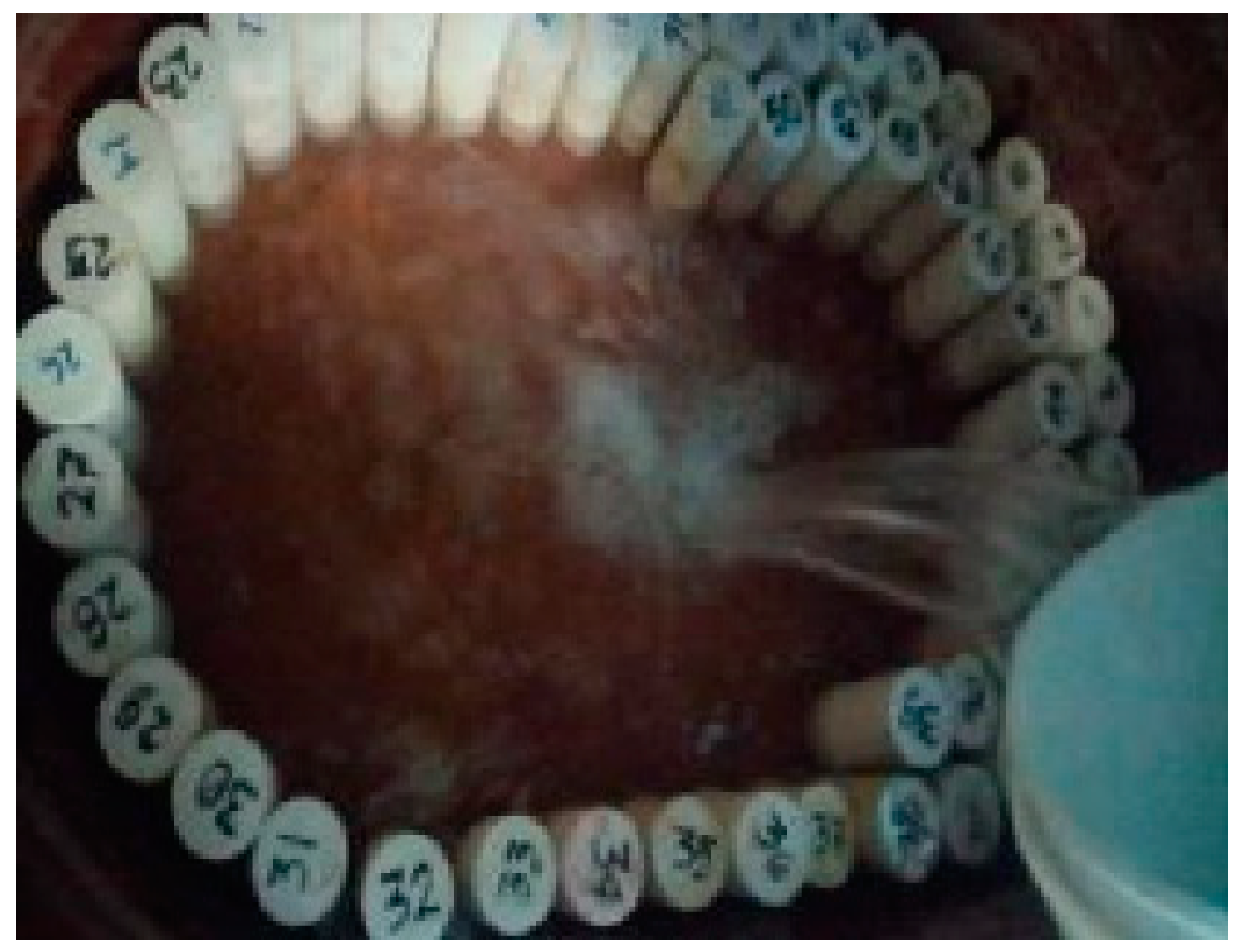
Rock cores were prepared and their dimensions and geometry verified in strict accordance with ASTM D4543-12 [37], which requires specimens to be straight, circular cylinders conforming to the following tolerances:
- Length-to-Diameter Ratio: Between 2.0 and 2.5.
- Minimum Diameter: [Specify análisi diameter in mm].
- End Surfaces: Cylinder end faces shall be lapped or polished to produce flat surfaces within a flatness tolerance of 0.00254 cm.
These preparations guarantee consistency and precision in all subsequent tests, as demonstrated in Figure 3.
To characterize the properties of the rock bench, the following sequence of laboratory tests was implemented:
- Uniaxial Compressive Strength (UCS)
The uniaxial compressive strength test (UCS) was performed according to ASTM D7012-10 [38]. The UCS was computed by dividing the peak axial load at failure by the specimen’s cross-sectional area.
Where:
- UCS = Uniaxial Compressive Strength
- P = Axial load
- A = Specimen’s cross-sectional area
Testing was carried out on a Model 2000 Universal Testing Machine (Serial No. 011065) using standard uniaxial compression protocols.
- Measure and record the specimen’s dimensions to calculate its cross-sectional area.
- Verify that the Universal Testing Machine is properly zeroed and configured before testing.
- Position the specimen centrally between the compression platens as shown in Figure 4.
- Use the machine control software to define the test parameters and initiate the compression sequence.
- Apply the axial load gradually at a constant rate until specimen failure.
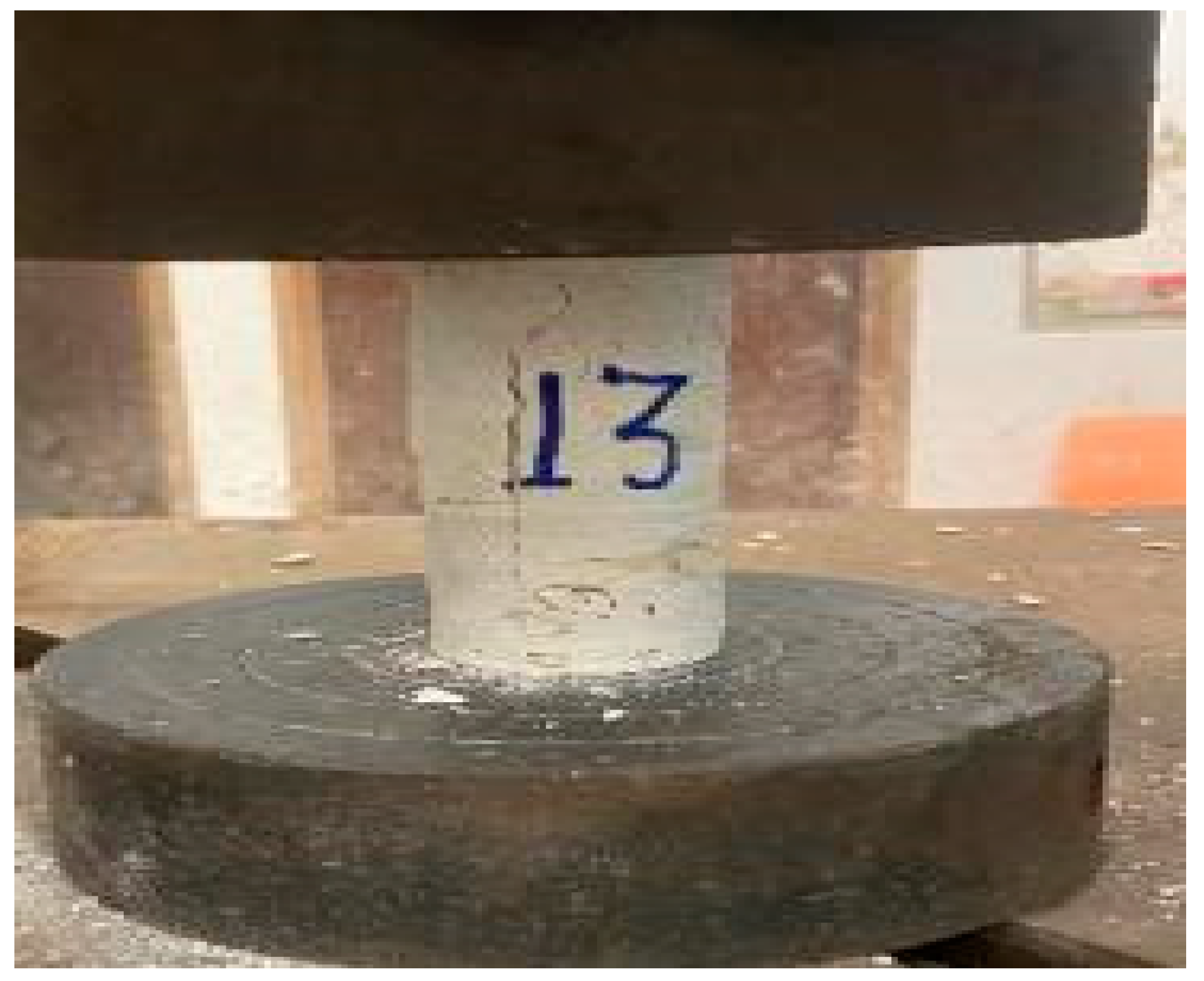
- Load the specimen to failure, as evidenced by crack initiation as illustrated in Figure 5.
- Upon failure, remove the specimen, install a fresh sample, and repeat the procedure.
Figure 4.
The specimen is positioned at the center of the compression platens in the Universal Testing Machine.
Figure 4.
The specimen is positioned at the center of the compression platens in the Universal Testing Machine.
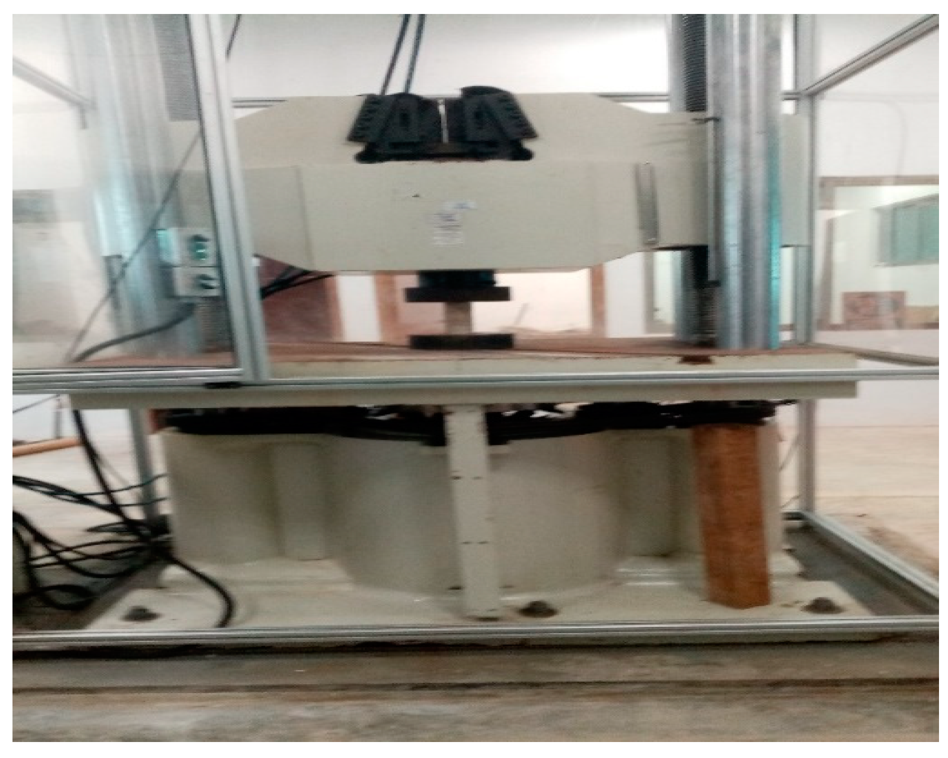
Figure 5.
Compression Test in Progress.
- Water Content
This test determines the rock’s in-situ moisture content—an indicator of retained water influenced by bench conditions, ambient humidity, and pore connectivity—according to ASTM D2216-10 [39], as shown in Figure 6.
Where:
- Pᵢ = initial (wet) mass of the sample, in grams
- Pf = final (oven-dry) mass of the sample, in grams
An average moisture content is calculated from multiple representative specimens. The step-by-step procedure for determining moisture content is as follows:
- Sample preparation
- Initial weighing (wet weight)
- Oven drying: maintain 105 ± 5 °C for 24 h
- Final weighing (dry weight)
- Calculation of análi content
Figure 6.
Procedure for determining the water content of Rock Samples.
- Real Density Test
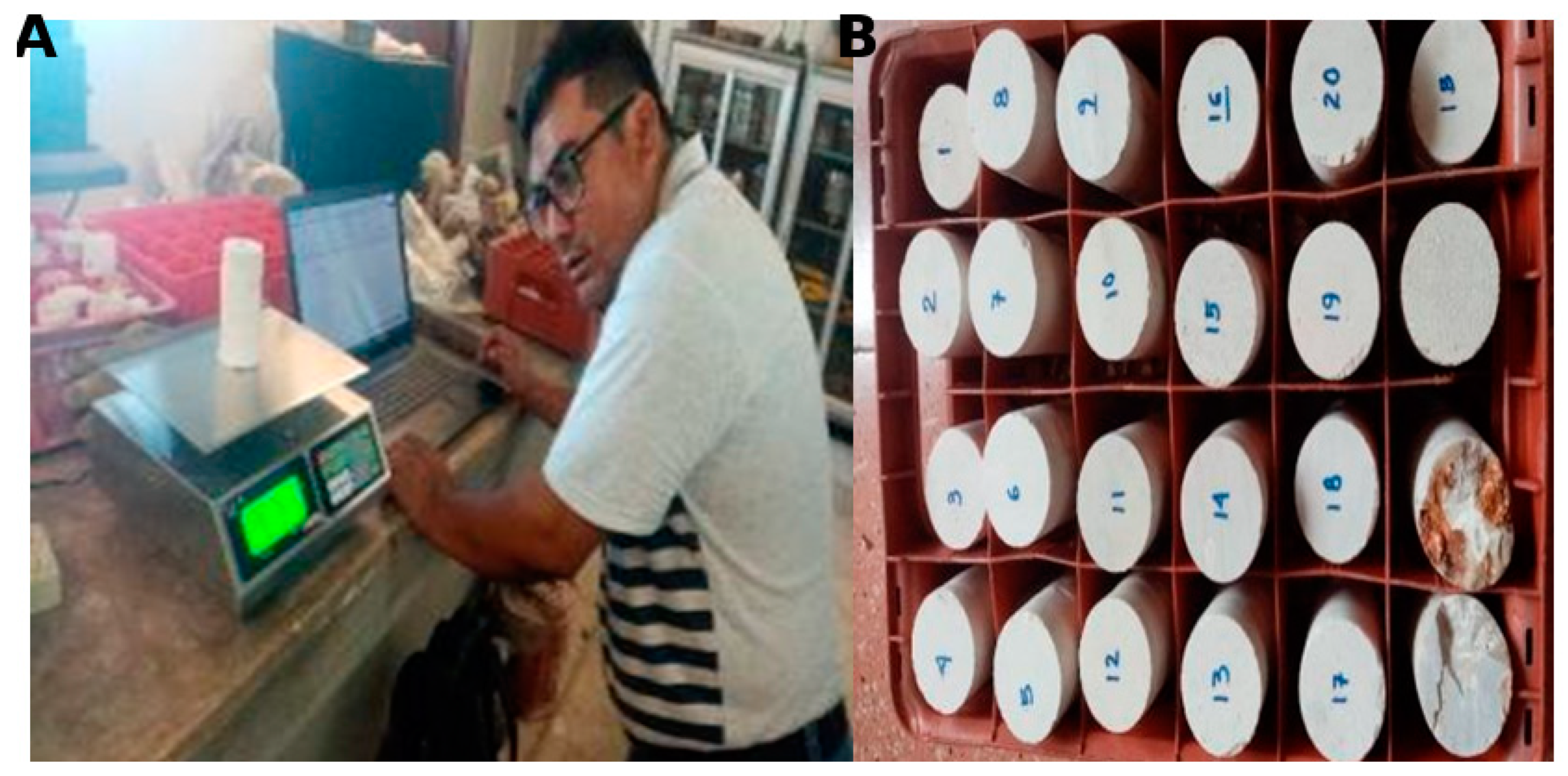
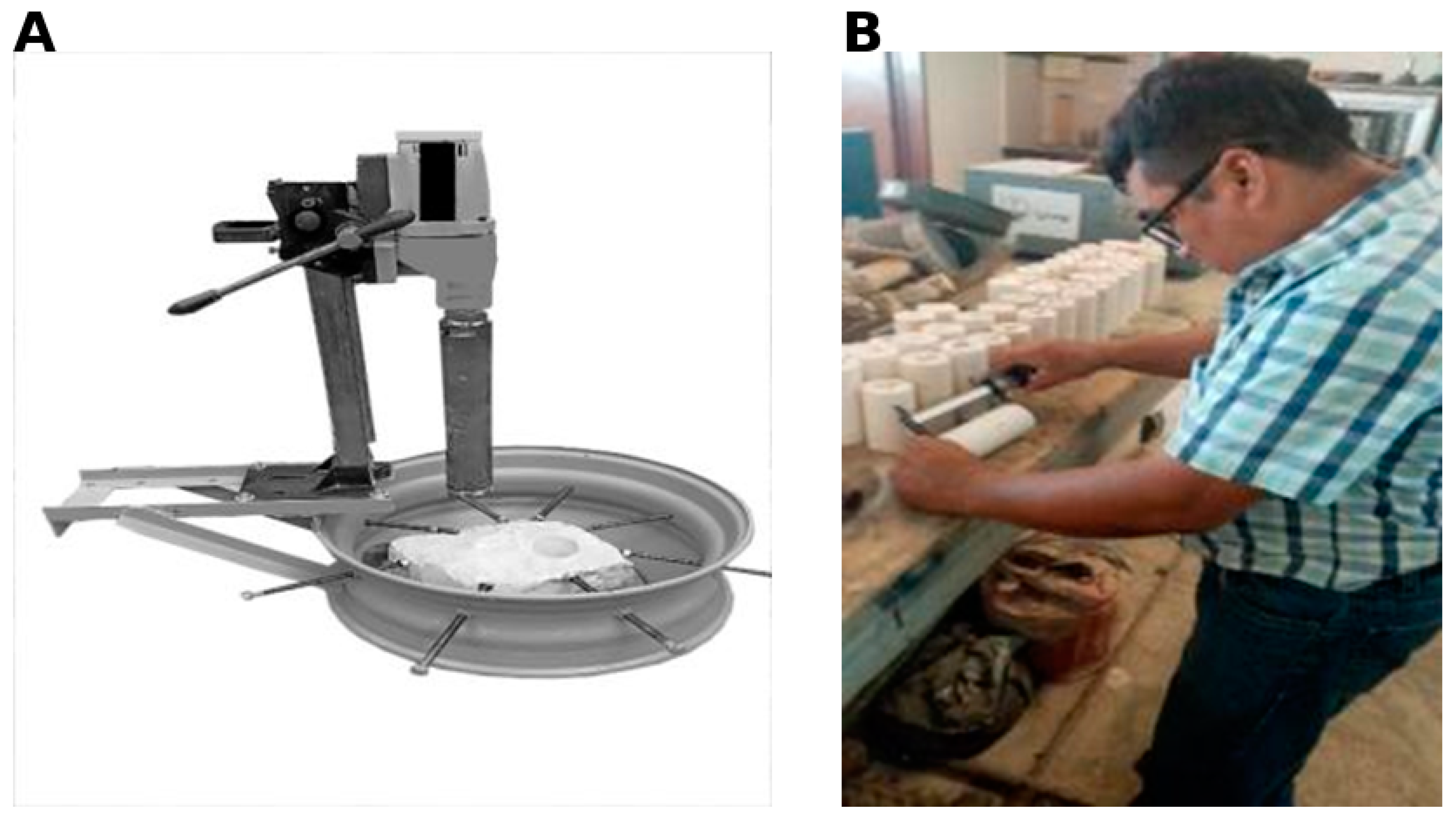
The real density of the rock was measured by ASTM D854-23 [40], as depicted in Figure 7. This method defines true density as the ratio of the specimen’s actual mass to its true volume and calculates it using the following equation:
Where:
- γ = real density (g/cm3)
- m = mass of the rock (g)
- V = comprehensive analysis of the specimen (cm³)
Nonetheless, the procedures for determining the rock’s true density
- Weigh the sample and record its mass (m) in grams
- Measure and record the sample volume (V) in cubic centimeters (cm³)
Figure 7.
Real density determination of rock specimens: (A) measurement of specimen mass; (B) determination of specimen volume.
Figure 7.
Real density determination of rock specimens: (A) measurement of specimen mass; (B) determination of specimen volume.
- Interconnected porosity
ASTM D4404-18 [41] – [42] specify the standard procedure for determining rock porosity, as visualized in Figure 8, expressed by the following equation:
Where:
- Pore volume (Vₚ) = volume of fluid absorbed by the rock sample
- Total volume (Vₜ) = the rock sample’s overall volumen
Figure 8.
Determination of interconnected porosity: (A) measurement of pore volume via fluid uptake; (B) determination of total sample volume.
Figure 8.
Determination of interconnected porosity: (A) measurement of pore volume via fluid uptake; (B) determination of total sample volume.
- Database
Tests were performed on 50 cylindrical specimens (diameter = 5.08 cm; length-to-diameter ratio = 2–2.5), and for each sample we recorded uniaxial compressive strength (UCS, MPa), moisture content (%), real density (g/cm³), and porosity (%) [43].
4. Neural Network Architectures for Uniaxial Compressive Strength Prediction
We implemented and compared four feed-forward neural network architectures to capture the complex, nonlinear dependence of uniaxial compressive strength (UCS) on water content, porosity, and density. Each model employs a distinct training algorithm and regularization scheme, which allows for a systematic evaluation of their convergence rates, generalization performance, and robustness to measurement noise:
- ✓
-
Radial Basis Function (RBF) Neural NetworkAn RBF network is a single-hidden-layer feed-forward model that uses Gaussian basis functions centered on training patterns. Hidden neurons are added incrementally until a performance goal on the training set is achieved, and the output layer linearly combines these localized responses to predict UCS. RBFs train quickly and model highly non-linear mappings, but they require careful tuning of the spread parameter to balance bias and variance [44].
- ✓
-
Bayesian Regularized Feed-Forward Neural NetworkThis approach incorporates weight decay into a Bayesian framework, ensuring that the objective minimizes both squared error and a complexity term. By utilizing the Levenberg–Marquardt algorithm, hyperparameters that govern the balance between error and weight penalty are updated during training, resulting in smoother, more generalizable models without a held-out validation set. This method is particularly effective with noisy or limited data, albeit at the expense of increased per-epoch computation [45].
- ✓
-
Scaled Conjugate Gradient (SCG) Neural NetworkSCG is a second-order method that scales conjugate gradient directions using approximate curvature information, avoiding expensive line searches, thus converging faster than simple gradient descent. In practice, a one-hidden-layer net (15 neurons) is trained over 1,000 epochs with a 70% train / 15% validation / 15% test. SCG balances speed and robustness for moderate-sized problems [46].
- ✓
-
Levenberg–Marquardt (LM) Neural NetworkLM blends Gauss–Newton and gradient-descent updates by adjusting a damping parameter μ: it reduces μ when the quadratic approximation holds and increases it when steps overshoot. When applied to a 15-neuron hidden layer, it typically converges in far fewer epochs than first-order methods. Regularization can be added for stability; however, its high memory demands limit the use of very large networks [47].
5. Performance Evaluation Metrics
To assess the accuracy of our machine-learning models, we employ four standard measures: Mean Absolute Error (MAE), Mean Square Error (MSE), Mean Absolute Percentage Error (MAPE), and the Coefficient of Determination (COD).
- Mean Absolute Error (MAE)
This metric captures the average absolute difference between predicted values and their authentic counterparts [48]. It is defined as:
Here, denotes the observed (true) value, represents the model’s predicted value, and is the total number of observations.
- Root Mean Square Error (RMSE)
RMSE measures the square root of the average squared deviations between predictions and observations [49]:
- Mean Absolute Percentage Error (MAPE)
MAPE expresses the average absolute error as a percentage of the true values and its predicted values [50], is calculated as:
- Coefficient of Determination (COD)
Also known as R2 indicates the fraction of the variance in the dependent variable that is predictable from the independent variables [51]. It is calculated by:
6. Results and Discussion
6.1. Descriptive Statistics of the Experimental Dataset Variables
Table 2 presents the descriptive statistics for the water content (%), interconnected porosity (%), real density (g/cm³), and uniaxial compressive strength (UCS, MPa). The mean of water content is 6.707 % (SD = 2.335 %), ranging from 3.73 % to 13.62 %, which indicates moderate variability in sample moisture levels. Interconnected porosity averages 15.459 % (SD = 4.377 %), with values spanning 9.73 % to 28.46 %, reflecting heterogeneity of specimens. Real density shows a tight distribution (mean = 2.352 g/cm³, SD = 0.159 g/cm³; min = 1.91 g/cm³, max = 2.62 g/cm³), suggesting relatively consistent lithological composition. UCS exhibits considerable (mean = 40.14 MPa, SD = 7.914 MPa; min = 11.4 MPa, max = 54.17 MPa), underscoring a wide range of mechanical strength. The interquartile ranges—water content (5.00–7.552 %), porosity (12.35–17.168 %), density (2.262–2.478 g/cm³), and UCS (34.932–44.845 MPa), further illustrate the data distribution and substantiate the inclusion of all four variables in the subsequent machine-learning models.
However, Figure 9 illustrates the frequency distributions of the four principal variables—moisture content, interconnected porosity, real density, and uniaxial compressive strength (UCS)—employed in this study.
- Water Content (%): The moisture content exhibits an approximately bell-shaped distribution centered at 6–7 %, with the majority (≈70 %) falling between 4 % and 9 %. A slight rightward skew is apparent, as a small number of specimens reach up to 13–14 %. This skew suggests occasional high-moisture outliers, which may influence rock weakening.
- Interconnected Porosity (%): Porosity values are concentrated between 10 % and 20 %, peaking around 12–15 %. The distribution is mildly right-skewed, with a tail extending toward 28 %, indicating that most rocks share similar characteristics, while a few exhibit significantly higher void space.
- Real Density (g/cm³): Density measurements cluster tightly between 2.2 and 2.5 g/cm³, with a modal of 2.3–2.4 g/cm³ and very few values below 2.1 g/cm³ or above 2.6 g/cm³. This narrow spread reflects a relatively homogeneous lithology across the rock bank.
- Uniaxial Compressive Strength (UCS, MPa): The strength distribution spans 11 MPa to 60 MPa, with about ≈75 % between 30 MPa and 50 MPa. The histogram shows a mild right skew, driven by a few robust specimens. The central tendency around 35–45 MPa underscores the variability in mechanical resistance, which is essential for robust predictive modeling.
Overall, these histograms reveal that real density is relatively uniform. In contrast, water content, porosity, and UCS exhibit greater variability and mild skewness—distributional characteristics that underscore the need for machine learning algorithms capable of modeling nonlinear relationships and robustly handling outliers in our predictive framework.
Nevertheless, Figure 10 depicts the pairwise relationships among water content (%), interconnected porosity (%), real density (g/cm³), and uniaxial compressive strength (UCS, MPa) in a matrix of scatterplots with histograms on the diagonal. The following observations emerge:
- Diagonal Histograms
- ◦
- Water Content concentrates between 4 % and 9 %, confirming the moderate moisture range noted previously.
- ◦
- Porosity predominantly ranges from 12 % to 17 %, with only a few samples exhibiting values above 25 %.
- ◦
- Density is tightly clustered near 2.3–2.5 g/cm³.
- ◦
- UCS shows a dominant band from 30 MPa to 50 MPa, matching the earlier histogram.
- Water Content vs. Porosity
- ◦
- A strong positive linear (r ≈ 0.85) indicates that wetter specimens tend to exhibit higher porosity, likely reflecting pore-filling by moisture (upper-left scatter).
- Water Content vs. Density
- ◦
- A moderate negative correlation (r ≈ –0.65) indicates that samples with higher moisture content generally exhibit lower dry density (lower-left cluster on the scatter plot), as expected when porosity increases
- Water Content vs. UCS
- ◦
- A weak to moderate negative correlation indicates that higher moisture content is generally associated with reduced mechanical strength; However, the considerable scatter suggests that additional factors also affect UCS.
- Porosity vs. Density
- ◦
- Porosity and density are inversely related (r ≈ –0.72), confirming that greater void space corresponds to lower bulk density (second-row, first-column scatter).
- Porosity vs. UCS
- ◦
- A negative correlation (r ≈ –0.78) indicates that samples with higher porosity exhibit lower UCS, underscoring porosity’s critical role in strength reduction.
- Density vs. UCS
- ◦
- A strong positive correlation (r ≈ 0.80) indicates that denser rocks resist compressive loading more effectively, making density one of the most predictive features for UCS (bottom-right scatter).
These pairwise patterns confirm the expected geomechanical interdependencies—moisture and porosity weaken the rock, whereas density enhances strength—and validate the selection of these four variables as primary inputs for subsequent machine learning models.
At the same time, Figure 11 presents the pairwise Pearson correlation coefficients between moisture content (%), interconnected porosity (%), real density (g/cm³), and uniaxial compressive strength (UCS, MPa). The color-coded matrix, with overlaid coefficient values, highlights the following key relationships:
- Water Content vs. Porosity (r = 0.992): A near-perfect positive correlation indicates that specimens with higher moisture content exhibit increased interconnected porosity, reflecting the pore network’s enhanced fluid-retention capacity.
- Moisture Content vs. Real Density (r = –0.861): A strong inverse relationship indicates that specimens retaining more moisture exhibit lower density, consistent with increased pore volume reducing the mass per unit volume.
- Moisture Content vs. UCS (r = –0.649): A moderate inverse correlation indicates that higher moisture content typically reduces compressive strength, although additional factors also influence UCS variability.
- Porosity vs. Density (r = –0.805): Porosity and density are strongly inversely related, confirming that increased void fraction corresponds to reduced material compactness.
- Porosity vs. UCS (r = –0.568): A moderate negative correlation indicates that increased porosity compromises compressive strength, underscoring pore structure as a primary weakening mechanism.
- Density vs. UCS (r = 0.929): A robust positive correlation indicates denser rocks resist compressive loading more effectively, making real density the most predictive univariate feature for UCS.
These findings validate the anticipated geomechanical interdependencies and support the inclusion of all four variables in our multivariate predictive models.
On the other hand, Figure 12 shows a parallel-coordinate plot with four vertical axes—water content (%), interconnected porosity (%), real density (g/cm³), and uniaxial compressive strength (UCS, MPa)—simultaneously mapping each sample’s values to highlight multidimensional relationships and sample heterogeneity.
- High-strength subset (rightmost lines): Samples with UCS > 45 MPa (the upper bundle on the right axis) consistently correspond to high real density (2.5–2.7 g/cm³) and low moisture content (3–6 %) and porosity (9–15 %), reaffirming that dense, low-porosity rocks exhibit superior compressive resistance.
- Low-strength subset: Samples with UCS < 25 MPa align with lower real density (1.9–2.2 g/cm³) and elevated moisture content (8–14 %) and porosity (18–28 %), highlighting how increased pore volume and moisture compromise compressive strength.
- Intermediate cluster: The majority of samples fall within mid-range values—moisture content 5–8 %, porosity 12–18 %, real density 2.3–2.5 g/cm³, and UCS 30–45 MPa—reflecting the dataset’s central tendency and confirming these intervals as representative for model training.
- Outliers: A few lines diverge sharply, such as one sample with exceptionally high porosity (>25 %) yet moderate UCS (~30 MPa), suggesting localized lithological variations or measurement anomalies worth further geological investigation.
Overall, the parallel coordinate plot visually confirms the inverse relationship between moisture content/porosity and density/UCS, clearly delineating distinct strength–density–porosity regimes that inform feature selection and stratified modeling strategies in our subsequent machine-learning workflows.
6.2. Model Implementation and Training Protocols
To ensure a fair comparison of four neural-network models for predicting uniaxial compressive strength (UCS) from moisture content, interconnected porosity, and real density, each algorithm was implemented in MATLAB using standardized preprocessing, consistent performance metrics, and carefully selected hyperparameters. Table 3 summarizes the data splits, network architectures, training functions, and evaluation metrics; detailed descriptions follow.
6.2.1. Radial Basis Function (RBF) Neural Network
Implemented with MATLAB’s newrb, the network grew hidden Gaussian units one at a time (up to 25) until the training MSE fell below 1 × 10⁻³ (spread = 0.8). Inputs were standardized (z-score) and outputs normalized to [0,1] via mapminmax. The model achieved R² = 0.972 and RMSE = 1.313 MPa on the hold-out set , as shown in Figure 13.
6.2.2. Bayesian Regularized Feed-Forward Neural Network
A single hidden-layer network (15 neurons) was trained using the Bayesian regularization function (trainbr), which balances squared error and applies automatic weight decay. Using the same 80/20 data split and preprocessing, the network was trained for up to 1,000 epochs and achieved on the test set: R² = 0.967, MAE = 1.164 MPa, and coefficient of determination (COD) = 0.967, as illustrated in Figure 14.
6.2.3. Scaled Conjugate Gradient (SCG) Neural Network
A 15-neuron feed-forward network was trained using the scaled conjugate gradient algorithm (trainscg) for up to 1,000 epochs, with early stopping on a 15 % validation subset. SCG accelerates convergence by scaling conjugate-gradient directions (λ₀ = 1 × 10⁻³, σ = 1 × 10⁻⁶) and incorporates a small regularization term (0.01). Training halted after 182 epochs, yielding R² = 0.964 and RMSE = 1.490 MPa, as presented in Figure 15.
6.2.4. Levenberg–Marquardt (LM) Neural Network
Using the Levenberg–Marquardt algorithm (trainlm) on a 70/15/15 data split, a 15-neuron network was trained for up to 1,000 epochs. This method blends Gauss–Newton and gradient-descent updates via an adaptive damping factor (μ₀ = 1 × 10⁻³, decrease factor = 0.1, increase factor = 10) and applies a weight-decay term of 0.1. The model converged after 25 epochs, achieving R² = 0.951 and RMSE = 1.737 MPa, as displayed in Figure 16.
6.2.5. Comparative Overview
Among the four architectures, the RBF network provided the best balance of accuracy (highest R², lowest RMSE/MAE) by automatically determining its topology and leveraging localized activations. The Bayesian model offered robust generalization via adaptive regularization without a separate validation set. SCG and LM delivered faster convergence and built-in regularization, but with slightly reduced predictive performance. This systematic implementation and evaluation framework ensures a transparent comparison of nonlinear modeling strategies for geomechanical data. Therefore, the RBF Neural Network delivers the best predictive accuracy about UCS. However, we must monitor validation performance because RBFs can overfit if the spread parameter is not well tuned. Nevertheless, the Bayesian-regularized is stronger for noisier data, trading off a bit of accuracy for added robustness as demonstrated in Table 4.
Nonetheless, Figure 17 presents boxplots of the mean squared error (MSE) distributions over 30 independent runs for each algorithm, showing the minimum, first quartile (Q1), median, third quartile (Q3), maximum, and outliers for both the training and testing sets. Table 5 complements these results by reporting each method’s median MSE on the training and test data.
Figure 17 demonstrates that the radial basis function (RBF) network performs best, exhibiting the lowest median MSE and the tightest interquartile range on training and testing data. The Bayesian-regularized (BR) network ranks second, with a slightly higher median error and moderate variability. The scaled conjugate gradient (SCG) network occupies third place, showing increased median MSE and greater spread, indicating sensitivity to data splits. The Levenberg–Marquardt (LM) network performs least favorably, with the highest median error and the broadest distribution. Crucially, the close correspondence between training and testing MSE across all four models suggests minimal overfitting.
To evaluate whether the observed differences in test-set MSE among the four neural-network algorithms were statistically significant, we applied the Friedman test with Benjamini–Hochberg correction [52] to all pairwise comparisons (Table 6). The null hypothesis for each comparison assumes equal median MSE; at α = 0.01, significant results are marked with an asterisk. The RBF network differed significantly from both the Bayesian-regularized model (adjusted p = 3.7 × 10⁻⁵) and the SCG model (adjusted p = 1.0 × 10⁻⁵). Similarly, BR (adjusted p = 2.0 × 10⁻⁴) and SCG (adjusted p = 1.6 × 10⁻⁴) outperformed the Levenberg–Marquardt network. In contrast, no significant differences were found between BR and SCG (adjusted p = 0.600) or between RBF and LM (adjusted p = 0.157), indicating comparable median performance for those pairs.
To further quantify predictive accuracy, we calculated the coefficient of determination (R²) from a linear regression of observed versus predicted values for each algorithm. Figure 18 presents boxplots of the R² distributions over 30 independent runs, showing the minimum, first quartile, median, third quartile, maximum, and outliers, for both training and testing sets. Table 7 complements this by reporting each method’s median R² on the training and test data.
These R² results corroborate the MSE findings: the RBF network achieves the highest median coefficient of determination, closely followed by the Bayesian-regularized model, both markedly outperforming the SCG and LM algorithms. In addition, we assessed statistical significance using the Friedman test with Benjamini–Hochberg correction, and the adjusted p-values in Table 8 confirm the conclusions drawn above.
6.2.6. Sensitivity Analysis
In order to quantify the relative influence of each geomechanical variable on our ANN’s uniaxial compressive strength (UCS) predictions, we conducted a sensitivity analysis using the partial derivatives (PD) method of Dimopoulos et al [53]. For each of the 30 independent network realizations, we computed the PD of the model output (predicted UCS) with respect to each input feature—water content, interconnected porosity, and real density— throughout all training runs. These derivatives were then averaged and normalized to yield percentage-based sensitivity scores, which are visualized in Figure 19. Interconnected porosity emerges as the dominant driver, accounting for 54.4 % of the model’s sensitivity, followed by water content at 30.9 % and real density at 14.7 %. This ranking underscores the preeminent role of porosity in controlling UCS within our ANN framework.
7. Summary, Conclusions, and Future Work
In this study, four feed-forward artificial neural network (ANN) architectures as Radial Basis Function (RBF), Bayesian Regularized (BR), Scaled Conjugate Gradient (SCG), and Levenberg–Marquardt (LM) were implemented and rigorously compared for predicting uniaxial compressive strength (UCS) of 50 Seybaplaya carbonate rock cores using water content, interconnected porosity, and real density as inputs.
- Key findings include:
Predictive Performance: The RBF network achieved the highest overall accuracy (median R² = 0.975; RMSE = 1.313 MPa) and significantly outperformed both BR and SCG models in test-set MSE (Friedman adjusted p < 0.01). Bayesian regularization yielded robust generalization (MAE = 1.164 MPa; R² = 0.967) without requiring a separate validation subset, while SCG and LM methods converged faster but showed slightly lower predictive power (Table 5 and Table 6).
Statistical Validation: Pairwise Friedman tests with Benjamini–Hochberg correction confirmed the RBF network’s superiority over BR and SCG, and demonstrated that BR and SCG both significantly outperform LM on median MSE (α = 0.01). No significant difference was observed between BR and SCG or between RBF and LM in specific comparisons, underscoring trade-offs among accuracy, convergence speed, and robustness.
Feature Sensitivity: Partial derivatives sensitivity analysis revealed that interconnected porosity is the dominant driver of UCS predictions (54.4 %), followed by water content (30.9 %) and real density (14.7 %). This prioritization aligns with geomechanical expectations in karst-influenced carbonates (Figure 21).
Conclusions
1. RBF networks—by automatically adapting topology and leveraging localized Gaussian activations—provide the most accurate data-driven framework for UCS estimation in heterogeneous carbonate formations.
2. Bayesian regularization offers a valuable balance of accuracy and noise resilience when data are limited and/or measurements are noisy.
3. SCG and LM methods remain attractive for applications requiring rapid convergence, though with a moderate sacrifice in predictive precision.
4. The sensitivity hierarchy (porosity > water content > density) informs sample characterization priorities and model interpretability in geotechnical practice.
- Future Work
Expanded Datasets & Lithologies: Validate and extend the comparative framework on larger, multi-site datasets encompassing diverse carbonate facies, clastic formations, and varying saturation conditions.
Hybrid & Deep Architectures: Investigate hybrid models (e.g., PSO-tuned ANNs, ANFIS, convolutional or graph-based networks) to capture spatiotemporal heterogeneities and improve generalization.
Field-Scale Integration: Couple ANN predictions with in situ geophysical logs (e.g., sonic, resistivity) and digital core imagery to enable real-time UCS estimation for tunneling, drilling, and reservoir stability assessments.
Uncertainty Quantification: Incorporate Bayesian inference, ensemble learning, or Monte Carlo dropout to quantify prediction uncertainties and support risk-based design decisions.
Model Deployment & Automation: Develop user-friendly software tools and automated workflows for practitioners to train, validate, and apply optimized ANN models within standard geotechnical engineering platforms.
Supplementary Materials
The following supporting information can be downloaded at the website of this paper posted on Preprints.org.
References
- Peng, J.; Zhang, K. Effects of Water Content on the Mechanical Behavior of Sedimentary Rocks. Rock Mechanics and Rock Engineering 2007,40 (2), 125–137.
- Freyburg, E. The Lower and Middle Buntsandstein of Southwest Thuringia in Its Geotechnical Properties. German Society for Geosciences, Series A, 176, 911–919 (1972).
- McNally, G. H. Estimation of Coal Measures Rock Strength Using Sonic and Density Logs. Log Analyst 1987, 28, 20–27.
- Galván, M.; Restrepo, I. Nonlinear Relationships between Water Saturation and Unconfined Compressive Strength in Limestones. International Journal of Rock Mechanics and Mining Sciences 2016, 84, 66–74.
- Gokceoglu, C. A Comparative Study of Neural Network and Multiple Regression Analysis in Modeling Rock Properties. Engineering Geology 2002, 66 (3–4), 281–295.
- Bieniawski, Z. T. Engineering Rock Mass Classifications: A Complete Manual for Engineers and Geologists in Mining, Civil, and Petroleum Engineering; Wiley: New York, NY, USA, 1975.
- ASTM International. ASTM D7012-10: Standard Test Method for Compressive Strength and Elastic Moduli of Intact Rock Core Specimens Under Varying States of Stress and Temperatures; ASTM International: West Conshohocken, PA, USA, 2010.
- Naal-Pech, A. Influence of Porosity and Density on the Compressive Strength of Seybaplaya Bank Rocks. Journal of Geotechnical Studies 2023,45 (3), 215–227.
- Chang, C.; Soon, T. H. R. Y.; McDougall, S. Porosity and Compressive Strength Relationships in Carbonates. Rock Mechanics and Rock Engineering 2006, 39 (5), 443–456.
- Naal-Pech, A. Extended Correlations for UCS Prediction in Karstic Limestones. In Proceedings of the 15th International Congress on Rock Mechanics; 2024; pp. 123–129.
- Fener, M.; Gül, E.; Ayday, O. Prediction of Uniaxial Compressive Strength Using Artificial Neural Networks. Environmental Geology 2005, 47 (1), 101–109.
- Naal-Pech, A.; Palemón-Arcos, L.; Gutiérrez-Can, Y.; El Hamzaoui, Y. Study of the Relationship between Uniaxial Compressive Strength vs. Non-Destructive Testing and Specific Weight in Bank Rocks from the Seybaplaya Campeche Mexico. J. Eng. Appl. 2024, 11, 16–25. [CrossRef]
- Peng, S.; Zhang, Z. Correlations of Compressive Strength (MPa) with Rock Physical Properties. Petroleum Science 2007, 4 (1), 67–73.
- Gokceoglu, C. A Neural Network Application to Estimate the Uniaxial Compressive Strength of Some Rocks from Their Petrographic Characteristics. Rock Mechanics and Rock Engineering 2002, 35 (3), 279–293.
- Lal, R. Shale Mechanical Properties and Crack Propagation. Journal of Petroleum Science 1999, 6 (3), 235–240.
- Chang, C.; Zoback, M. D.; Khaksar, A. Empirical Relationships between Compressive Strength and Porosity in Gulf of Mexico Rocks. SPE Journal 2006, 11 (1), 19–25.
- Naal-Pech, J. W.; Palemón-Arcos, L.; El Hamzaoui, Y.; Gutiérrez-Can, Y. Study of the Relationship between Uniaxial Compressive Strength and the Point Load Test in Rocks from the Bank in Seybaplaya Campeche Mexico. J. Eng. Appl. 2024,11(32), 36–42.
- Wei, X.; Shahani, N. M.; Zheng, X. Predictive Modeling of the Uniaxial Compressive Strength of Rocks Using an Artificial Neural Network Approach. Mathematics 2023, 11, 1650. [CrossRef]
- Torabi-Kaveh, M.; Naseri, F.; Saneie, S.; Sarshari, B. Application of Artificial Neural Networks and Multivariate Statistics to Predict UCS and E Using Physical Properties of Asmari Limestones. Arabian Journal of Geosciences 2015,8, 2889–2897. [CrossRef]
- Yagiz, S.; Sezer, E. A.; Gokceoglu, C. Artificial Neural Networks and Nonlinear Regression Techniques to Assess the Influence of Slake Durability Cycles on the Prediction of Uniaxial Compressive Strength and Modulus of Elasticity for Carbonate Rocks. Int. J. Numer. Anal. Meth. Geomech. 2012, 36, 1636–1650. [CrossRef]
- Setayeshirad, M. R.; Uromeie, A.; Nikudel, M. R. Modeling of the Uniaxial Compressive Strength of Carbonate Rocks Using Statistical Analysis and Artificial Neural Network. Rock Mech. Rock Eng. 2025, . [CrossRef]
- Ceryan, N.; Okkan, U.; Kesimal, A. Prediction of Unconfined Compressive Strength of Carbonate Rocks Using Artificial Neural Networks. Environmental Earth Sciences 2013, 68, 807–819.https://. [CrossRef]
- Abdi, Y.; Taheri-Garavand, A. Application of the ANFIS Approach for Estimating the Mechanical Properties of Sandstones. Emirates Journal of Engineering Research 2020, 25 (4), 1–19.
- Umrao, R. K.; Sharma, L. K.; Singh, R.; Singh, T. N. Determination of Strength and Modulus of Elasticity of Heterogeneous Sedimentary Rocks: An ANFIS Predictive Technique. Measurement 2018, 126, 194–201. [CrossRef]
- Cabalar, A. F.; Cevik, A.; Gokceoglu, C. Some Applications of Adaptive Neuro-Fuzzy Inference System (ANFIS) in Geotechnical Engineering. Computers and Geotechnics 2012, 40, 14–33. [CrossRef]
- Mohamad, E. T.; Jahed Armaghani, D.; Momeni, E.; Alavi Nezhad Khalil Abad, S. V. Prediction of the Unconfined Compressive Strength of Soft Rocks: A PSO-Based ANN Approach. Bulletin of Engineering Geology and the Environment 2015,74, 745–757. [CrossRef]
- Momeni, E.; Rashidi Khabir, R. A Reliable PSO-Based ANN Approach for Predicting Unconfined Compressive Strength of Sandstones. Open Construction and Building Technology Journal 2020, 14 (Suppl. 1, M5), 237–249. [CrossRef]
- Dehghan, S.; Sattari, G.H.; Chehreh, C.S.; Aliabadi, M.A. Prediction of Unconfined Compressive Strength and Modulus of Elasticity for Travertine Samples Using Regression and Artificial Neural Networks. Min. Sci. Technol. 2010, 20, 41–46.
- Kalkan, E.; Akbulut, S.; Tortum, A.; Celik, S. Prediction of the Unconfined Compressive Strength of Compacted Granular Soils by Using Inference Systems. Environmental Geology 2009, 58, 1429–1440. [CrossRef]
- Baykaşoğlu, A.; Güllü, H.; Çanakçı, H.; Özbakır, L. Prediction of Compressive and Tensile Strength of Limestone via Genetic Programming.Expert Systems with Applications 2008, 35, 111–123. [CrossRef]
- Xue, X.; Wei, Y. A Hybrid Modelling Approach for Prediction of Uniaxial Compressive Strength of Rock Materials. Comptes Rendus Mécanique 2020, 348, 235–243. [CrossRef]
- Gokceoglu, C.; Zorlu, K. A Fuzzy Model to Predict the Uniaxial Compressive Strength and the Modulus of Elasticity of a Problematic Rock. Engineering Applications of Artificial Intelligence 2004, 17, 61–72. [CrossRef]
- Khatti, J.; Grover, K. S. Estimation of Intact Rock Uniaxial Compressive Strength Using Advanced Machine Learning. Transportation Infrastructure Geotechnology 2024, 11, 1989–2022. [CrossRef]
- Sabri, M. S.; Jaiswal, A.; Verma, A. K.; Singh, T. N. Advanced Machine Learning Approaches for Uniaxial Compressive Strength Prediction of Indian Rocks Using Petrographic Properties. Multiscale Multidisciplinary Modeling Experiments and Design 2024, 7, 5265–5286. [CrossRef]
- Kochukrishnan, S.; Krishnamurthy, P.; Yuvarajan, D.; Kaliappan, N. Comprehensive Study on the Python-Based Regression Machine Learning Models for Prediction of Uniaxial Compressive Strength Using Multiple Parameters in Charnockite Rocks. Scientific Reports 2024, 14,7360. [CrossRef]
- Servicio Geológico Mexicano. Implementing the 1992 Mining Law: Analysis of Mineral Substances and Administration of Concessions; Servicio Geológico Mexicano: Mexico City, Mexico, 2021.
- ASTM International. ASTM D4543-12: Standard Practices for Preparing Rock Core as Cylindrical Test Specimens and Verifying Conformance to Dimensional and Shape Tolerances; ASTM International: West Conshohocken, PA, USA, 2012.
- ASTM International. ASTM D7012-10: Standard Test Method for Compressive Strength and Elastic Moduli of Intact Rock Core Specimens Under Varying States of Stress and Temperatures; ASTM International: West Conshohocken, PA, USA, 2010.
- ASTM International. ASTM D2216-10: Standard Test Methods for Laboratory Determination of Water (Moisture) Content of Soil and Rock by Mass; ASTM International: West Conshohocken, PA, USA, 2010.
- ASTM International. ASTM D854-23: Standard Test Methods for Specific Gravity of Soil Solids by the Water Displacement Method; ASTM International: West Conshohocken, PA, USA, 2023.
- ASTM International. ASTM D4404-18: Standard Test Method for Determination of Pore Volume and Pore Volume Distribution of Soil and Rock by Mercury Intrusion Porosimetry; ASTM International: West Conshohocken, PA, USA, 2018.
- Nieto, G. C.; Avendaño, D. P. Laboratory Guide for Material Strength Testing; Inimagdalena: Bogotá, D.C., Colombia, 2015.
- Naal-Pech, J. W.; Palemón-Arcos, L.; El Hamzaoui, Y.; Gutiérrez-Can, Y. Study of the Relationship between Uniaxial Compressive Strength, Water Content, Porosity and Density in Bank Rocks in Seybaplaya Campeche. J. Mech. Eng. 2023, 7, 9–16.
- Moody, C. J. C. H.; Darken, C. J. Fast Learning in Networks of Locally-Tuned Processing Units. Neural Computation 1989, 1 (2), 281–294.
- MacKay, D. J. C. Bayesian Interpolation. Neural Computation 1992, 4 (3), 415–447.
- Møller, M. F. A Scaled Conjugate Gradient Algorithm for Fast Supervised Learning. Neural Networks 1993, 6 (4), 525–533.
- Hagan, M. T.; Menhaj, M. R. Training Feedforward Networks with the Marquardt Algorithm. IEEE Trans. Neural Networks 1994, 5, 989–993.
- Uzuner, S.; Cekmecelioğlu, D. Comparison of Artificial Neural Networks (ANN) and Adaptive Neuro-Fuzzy Inference System (ANFIS) Models in Simulating Polygalacturonase Production. BioResources 2016, 11 (4), 8676–8685. [CrossRef]
- Sada, S. O.; Ikpeseni, S. C. Evaluation of ANN and ANFIS Modeling Ability in the Prediction of AISI 1050 Steel Machining Performance. Heliyon 2021,7 (2), e06136. [CrossRef]
- Zhang, G.; Patuwo, B. E.; Hu, M. Y. Forecasting with Artificial Neural Networks: The State of the Art. Int. J. Forecast. 1998, 14, 35–62.
- Chong, D. J. S.; Chan, Y. J.; Arumugasamy, S. K.; Yazdi, S. K.; Lim, J. W. Optimisation and Performance Evaluation of Response Surface Methodology (RSM), Artificial Neural Network (ANN) and Adaptive Neuro-Fuzzy Inference System (ANFIS) in the Prediction of Biogas Production from Palm Oil Mill Effluent (POME). Energy 2023, 266, 126449. [CrossRef]
- Friedman, J. H. Multivariate Adaptive Regression Splines. Ann. Stat. 1991, 19 (1), 1–67.
- Dimopoulos, I.; Bourret, P.; Lek, S. Use of Some Sensitivity Criteria for Choosing Networks with Good Generalization Ability. Neural Processing Letters 1995, 2 , 1–4.
Figure 1.
Geological context of the Seybaplaya Formation: (a) Regional location within Campeche, Mexico; (b) State-scale geological map.
Figure 1.
Geological context of the Seybaplaya Formation: (a) Regional location within Campeche, Mexico; (b) State-scale geological map.
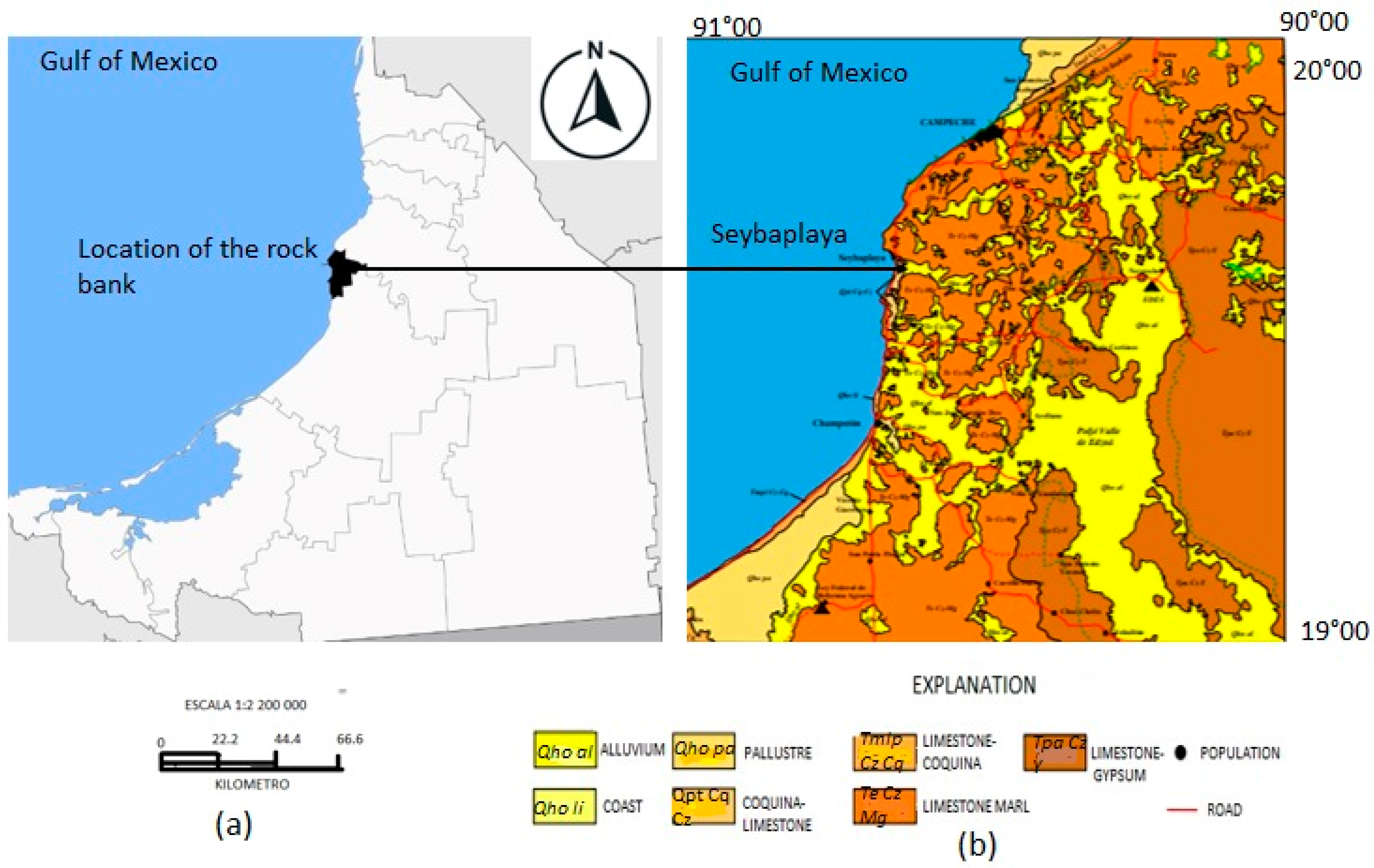
Figure 2.
Seybaplaya bank rocks.
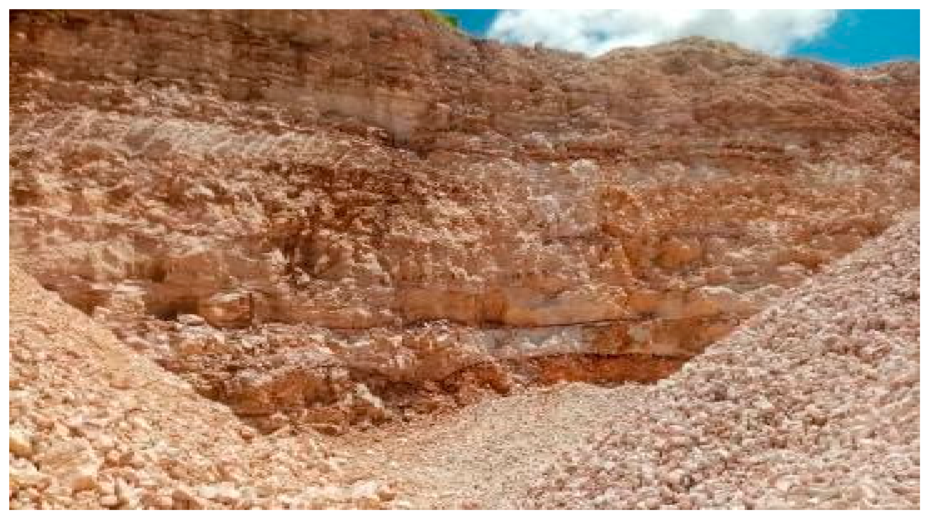
Figure 3.
Array of straight, circular, cylindrical rock specimens prepared for mechanical testing.
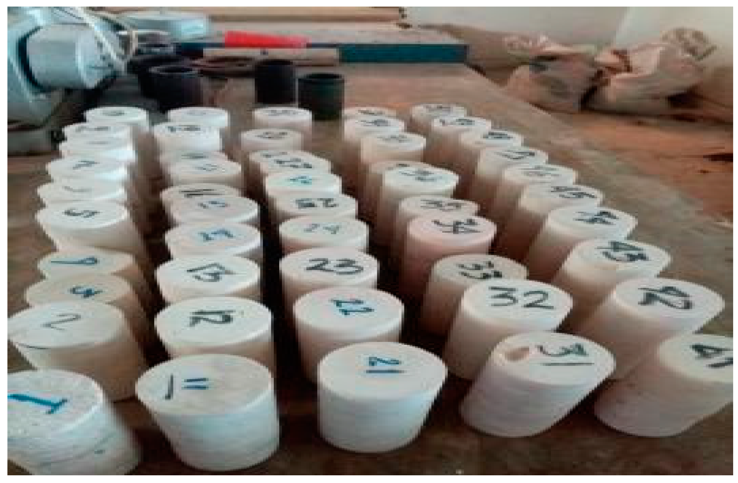
Figure 9.
Plot of the properties of Seybaplaya Bank Rocks.
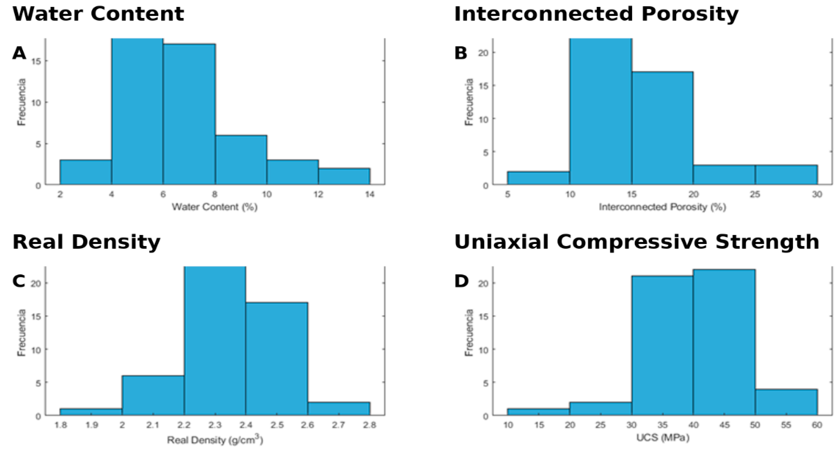
Figure 10.
Pair plot of the database.
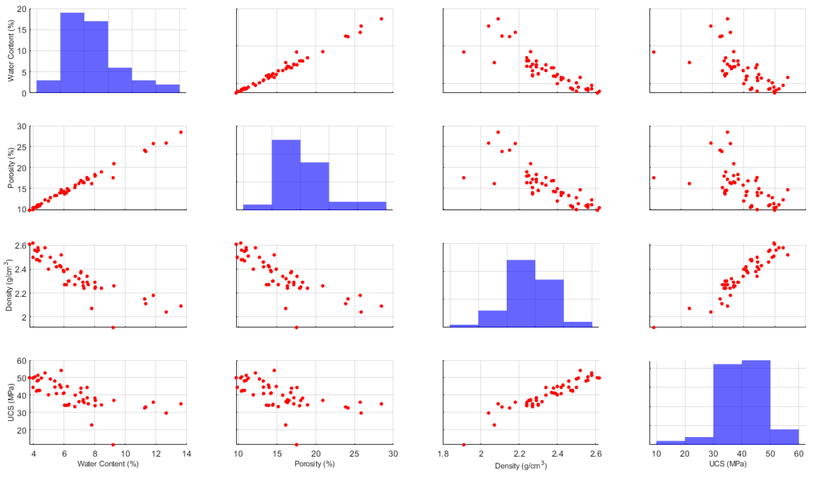
Figure 11.
Pearson correlation coefficient heatmap for rock properties.
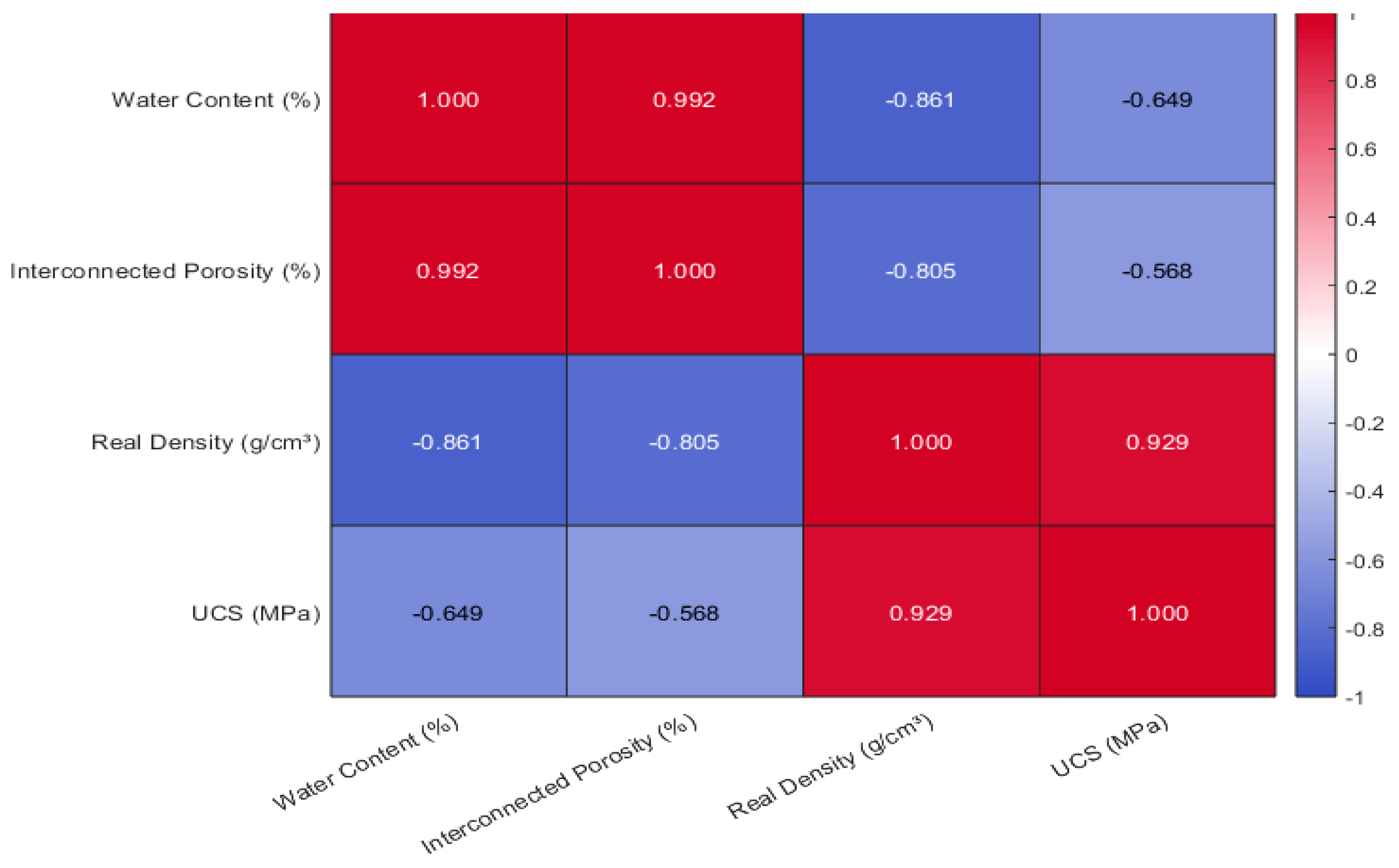
Figure 12.
Parallel coordinate plot of rock properties.
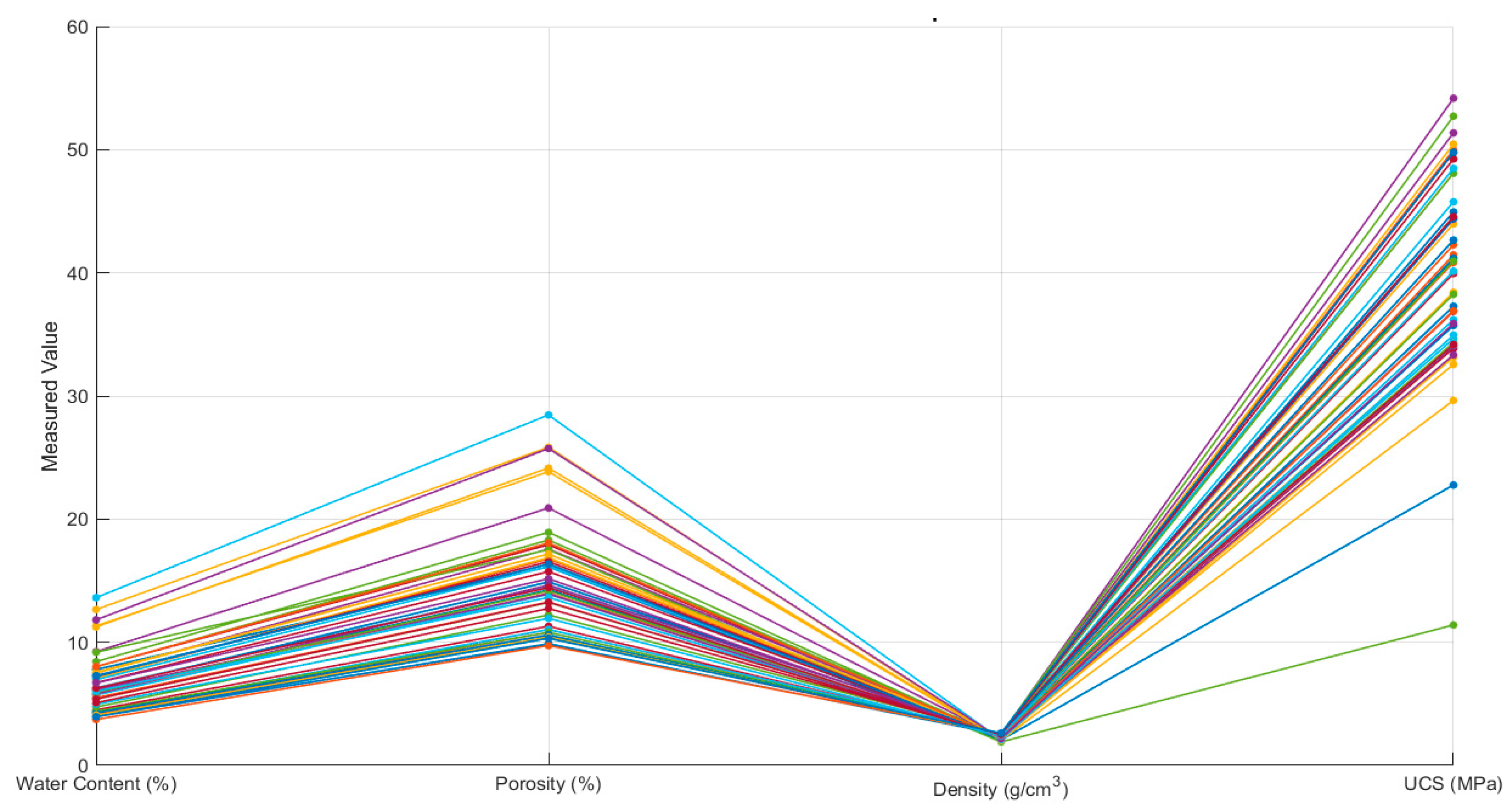
Figure 13.
Comparison of Actual vs. Predicted UCS: Radial Basis Function Neural Network (spread = 0.8; max neurons = 25; RMSE = 1.313 Mpa; R² = 0.972).
Figure 13.
Comparison of Actual vs. Predicted UCS: Radial Basis Function Neural Network (spread = 0.8; max neurons = 25; RMSE = 1.313 Mpa; R² = 0.972).

Figure 14.
Comparison of Actual vs. Predicted UCS: Bayesian Regularized Neural Network (15 neurons; 1000 epochs; MAE = 1.164 Mpa; COD = 0.967).
Figure 14.
Comparison of Actual vs. Predicted UCS: Bayesian Regularized Neural Network (15 neurons; 1000 epochs; MAE = 1.164 Mpa; COD = 0.967).
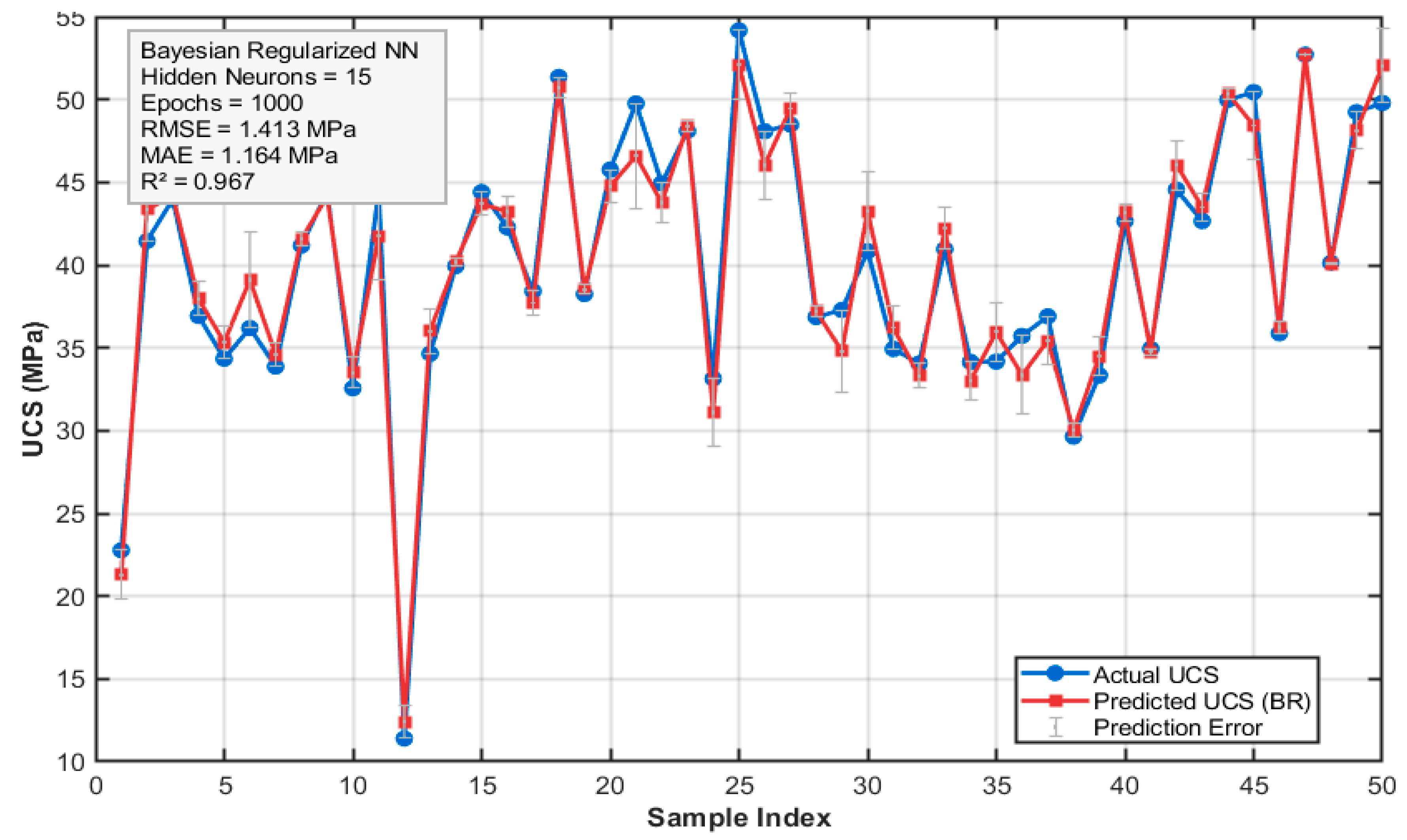
Figure 15.
Comparison of Actual vs. Predicted UCS: Scaled Conjugate Gradient Neural Network (15 neurons; λ₀ = 1e-3; σ = 1e-6; RMSE = 1.490 MPa; R² = 0.964).
Figure 15.
Comparison of Actual vs. Predicted UCS: Scaled Conjugate Gradient Neural Network (15 neurons; λ₀ = 1e-3; σ = 1e-6; RMSE = 1.490 MPa; R² = 0.964).
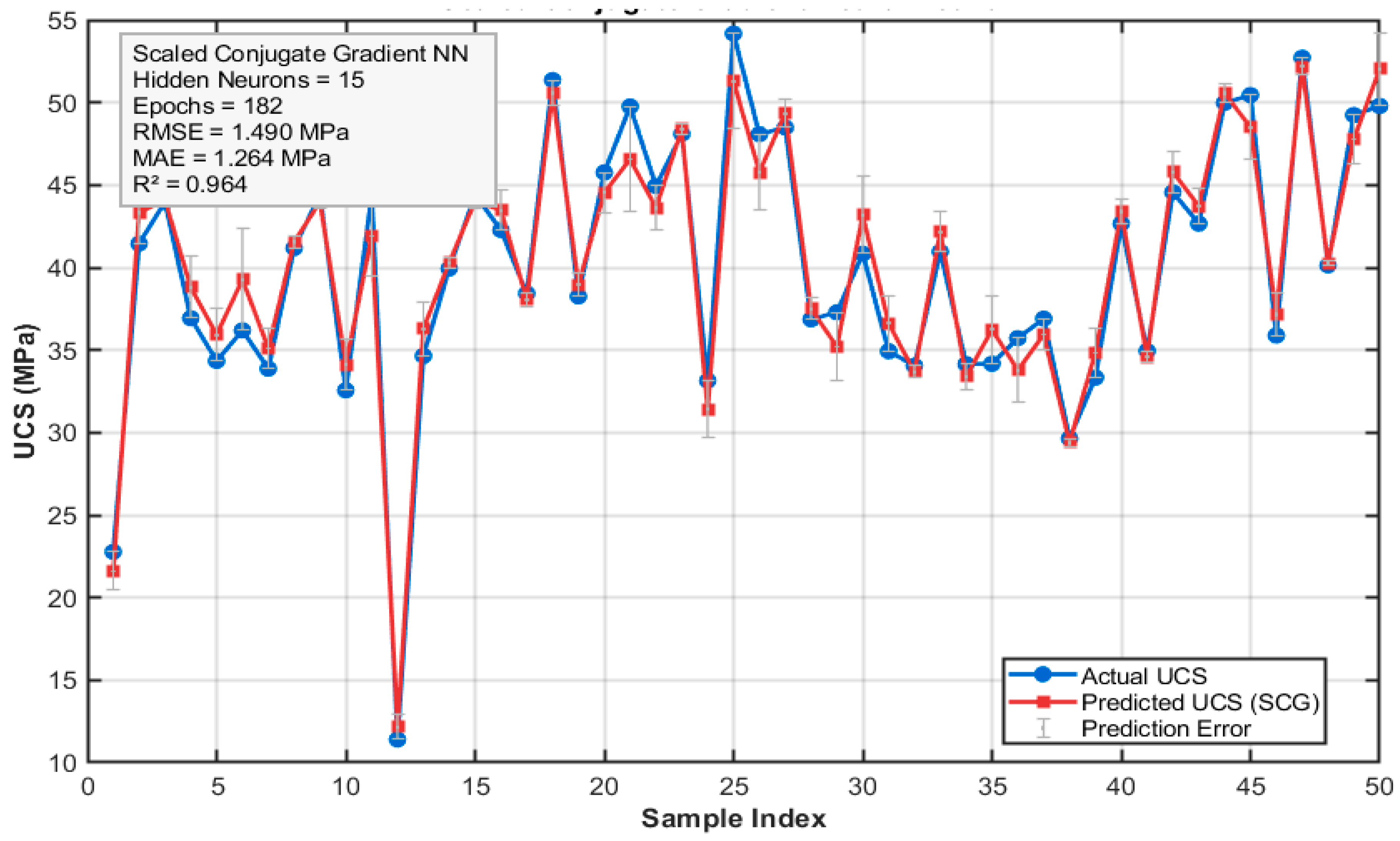
Figure 16.
Comparison of Actual vs. Predicted UCS: Levenberg–Marquardt Neural Network (15 neurons; μ₀ = 1e-3; 25 epochs; RMSE = 1.737 Mpa; R² = 0.951).
Figure 16.
Comparison of Actual vs. Predicted UCS: Levenberg–Marquardt Neural Network (15 neurons; μ₀ = 1e-3; 25 epochs; RMSE = 1.737 Mpa; R² = 0.951).

Figure 17.
Comparison of Mean Squared Error on Training and Testing Sets Across Neural Network Algorithms.
Figure 17.
Comparison of Mean Squared Error on Training and Testing Sets Across Neural Network Algorithms.
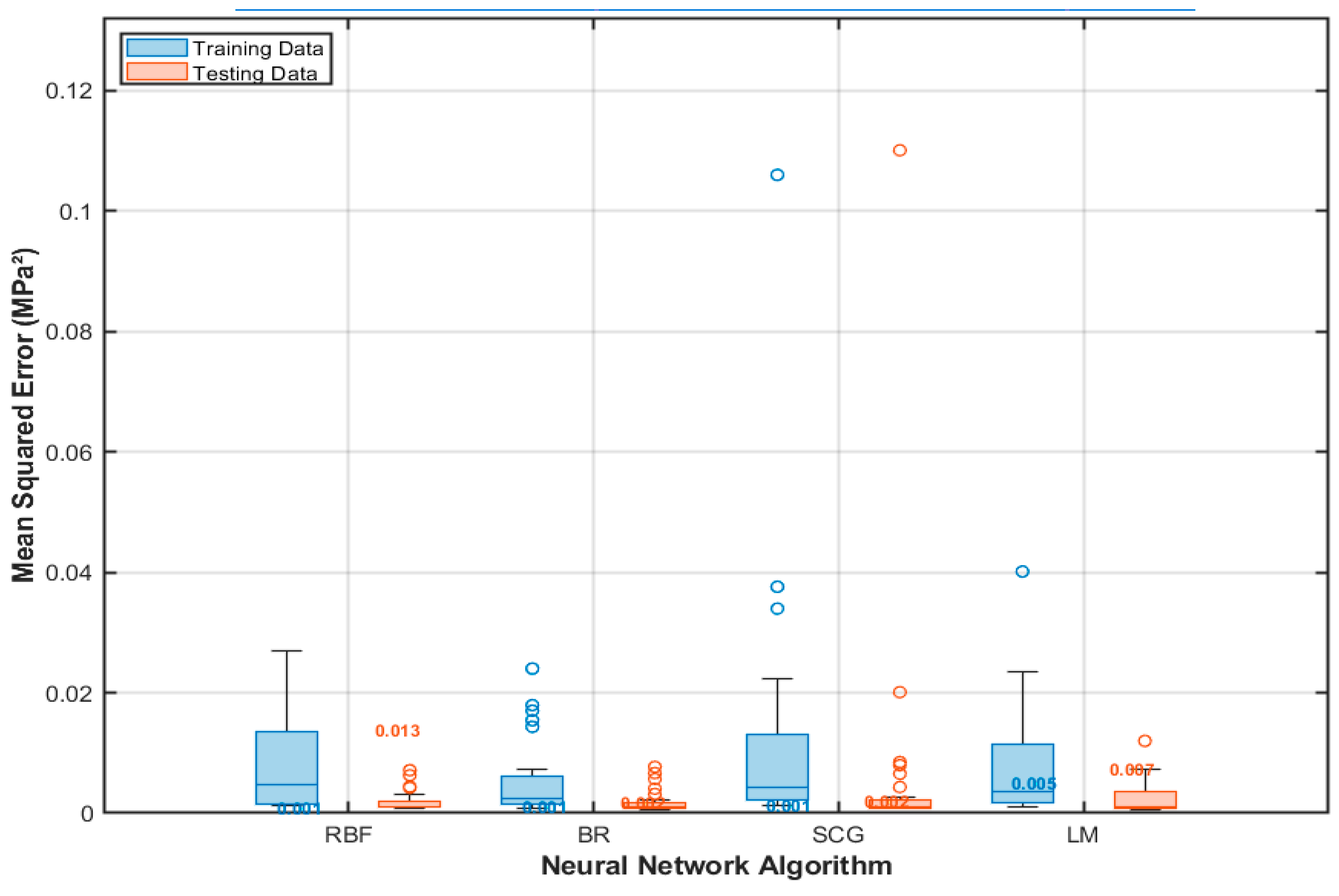
Figure 18.
Comparison of R2 on Training and Testing Sets Across Neural Network Algorithms.

Figure 19.
Relative contribution of input features to uniaxial compressive strength predictions.
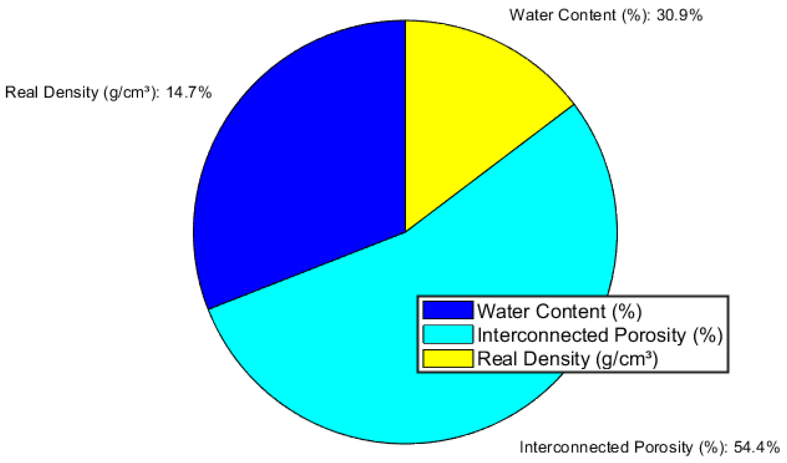

Table 1.
Location of the 50 Samples.
| Sample Range | UTM Coordinates (X, Y) |
| Samples 1–10 | (741595, 2174717) |
| Samples 11–20 | (741611, 2174838) |
| Samples 21–30 | (741585, 2174851) |
| Samples 31–40 | (741591, 2174750) |
| Samples 41–50 | (741605, 2174803) |
Table 2.
Descriptive Statistics of Input Features (Water Content, Porosity, Density) and Target UCS for Neural-Network Modeling.
Table 2.
Descriptive Statistics of Input Features (Water Content, Porosity, Density) and Target UCS for Neural-Network Modeling.
| WaterContent | InterconectedPorosity | RealDensity | UCS | |
| Mean | 6.707 | 15.459 | 2.352 | 40.14 |
| Std_dev | 2.335 | 4.377 | 0.159 | 7.914 |
| Min | 3.73 | 9.73 | 1.91 | 11.4 |
| 1st_quartil | 5.0 | 12.35 | 2.262 | 34.932 |
| Median | 6.235 | 14.565 | 2.355 | 40.485 |
| 3rd_quartile | 7.552 | 17.168 | 2.478 | 44.845 |
| Max | 13.62 | 28.46 | 2.62 | 54.17 |
Table 3.
Summary of Model Configurations, Training Functions, and Evaluation Criteria.
| Model | MATLAB Function | Topology | Data Split | Preprocessing | Key Hyperparameters | Performance Metrics |
| RBF Network | newrb | Up to 25 Gaussian units | 80 % train / 20 % test | Inputs z-score; outputs mapminmax [0,1] | Spread = 0.8; goal MSE = 1×10⁻³ | RMSE, R² |
| Bayesian Regularized NN | trainbr | 1 hidden layer, 15 neurons | 80 % / 20 % | z-score; mapminmax | Max epochs = 1 000; α,β auto-tuned | MAE, COD |
| SCG Network | trainscg | 1 hidden layer, 15 neurons | 70 % / 15 % / 15 % | z-score; mapminmax | λ₀ = 1e-3; σ = 1e-6; reg = 0.01 | RMSE, MAPE |
| LM Network | trainlm | 1 hidden layer, 15 neurons | 70 % / 15 % / 15 % | z-score; mapminmax | μ₀ = 1e-3; μ↓ = 0.1; μ↑ = 10; reg = 0.1 | COD, RMSE |
Table 4.
Aggregate Performance Metrics Over 30 Runs for All Neural-Network Models.
| Algorithm | R² | RMSE (MPa) | MAE (MPa) |
| RBF Neural Network | 0.972 | 1.313 | 1.029 |
| Bayesian Regularized Neural Network | 0.967 | 1.413 | 1.164 |
| Scaled Conjugate Gradient Neural Network | 0.964 | 1.490 | 1.264 |
| Levenberg–Marquardt Neural Network | 0.951 | 1.737 | 1.453 |
Table 5.
Summary of MSE by each algorithm on the training and testing sets, showing the median (30 runs).
Table 5.
Summary of MSE by each algorithm on the training and testing sets, showing the median (30 runs).
| Algorithm | Median MSE_Train | Median MSE_Test |
| RBF | 0.0008 | 0.0128 |
| Bayesian | 0.0010 | 0.0017 |
| SCG | 0.0013 | 0.0019 |
| LM | 0.0046 | 0.0068 |
Table 6.
Pairwise Friedman test results for test-set MSE with Benjamini–Hochberg correction. Raw and adjusted p-values are reported; an asterisk (*) denotes rejection of the null hypothesis at the α = 0.01 level.
Table 6.
Pairwise Friedman test results for test-set MSE with Benjamini–Hochberg correction. Raw and adjusted p-values are reported; an asterisk (*) denotes rejection of the null hypothesis at the α = 0.01 level.
| Comparison | p-value | Adjusted (p) Significant |
| RBF vs BR | 0.000012 | 0.000037* |
| RBF vs SCG | 0.000002 | 0.000010* |
| RBF vs LM | 0.130592 | 0.156710* |
| BR vs SCG | 0.599936 | 0.599936 |
| BR vs LM | 0.000136 | 0.000204* |
| SCG vs LM | 0.000082 | 0.000164* |
* indicates significant difference at α = 0.01 level.
Table 7.
Summary of R2 by each algorithm on the training and testing sets, showing the median (30 runs).
Table 7.
Summary of R2 by each algorithm on the training and testing sets, showing the median (30 runs).
| Algorithm | Median R2_Train | Median R2_Test |
| RBF | 0.9753 | 0.5932 |
| Bayesian | 0.9690 | 0.9286 |
| SCG | 0.9575 | 0.9274 |
| LM | 0.8532 | 0.8043 |
Table 8.
Pairwise Friedman test results for test-set MSE with Benjamini–Hochberg correction. Raw and adjusted p-values are reported; an asterisk (*) denotes rejection of the null hypothesis at the α = 0.01 level.
Table 8.
Pairwise Friedman test results for test-set MSE with Benjamini–Hochberg correction. Raw and adjusted p-values are reported; an asterisk (*) denotes rejection of the null hypothesis at the α = 0.01 level.
| Comparison | p-value | Adjusted (p) Significant |
| RBF vs BR | 0.000006 | 0.000017* |
| RBF vs SCG | 0.000002 | 0.000010* |
| RBF vs LM | 0.059836 | 0.071803 |
| BR vs SCG | 0.530440 | 0.530440 |
| BR vs LM | 0.000075 | 0.000113* |
| SCG vs LM | 0.000063 | 0.000113* |
* indicates significant difference at α = 0.01 level.
Disclaimer/Publisher’s Note: The statements, opinions and data contained in all publications are solely those of the individual author(s) and contributor(s) and not of MDPI and/or the editor(s). MDPI and/or the editor(s) disclaim responsibility for any injury to people or property resulting from any ideas, methods, instructions or products referred to in the content. |
© 2025 by the authors. Licensee MDPI, Basel, Switzerland. This article is an open access article distributed under the terms and conditions of the Creative Commons Attribution (CC BY) license (http://creativecommons.org/licenses/by/4.0/).
Copyright: This open access article is published under a Creative Commons CC BY 4.0 license, which permit the free download, distribution, and reuse, provided that the author and preprint are cited in any reuse.


