
Submitted:
22 June 2023
Posted:
22 June 2023
You are already at the latest version
Abstract
The purpose of this work is to compare two fracture prediction models with real-world data. The pure Artificial Neural Network (ANN) model emphasizes regression analysis, while the hybrid model (SVM-ANN) focuses on the combination of regression and classification analysis or Support Vector Machine. The results were subsequently tested against logging data by combining the Machine Learning approach with advanced logging tools. In this context, we used electrical image logs and the dipole acoustic tool which together allowed the distinction of 404 open fractures and 231 closed fractures and, consequently the estimation of fracture porosity. The results are then fed into two machine-learning algorithms. Pure Artificial Neural Networks and hybrid models are used to establish comprehensive results, which are subsequently tested to check the accuracy of the models. The outputs obtained from the two methods demonstrate that the hybridized model has a lower Root Mean Square Error (RMSE) than pure ANN. The results of our approach strongly suggest that incorporating hybridized machine learning algorithms in fracture porosity estimations can contribute to the development of more trustworthy static reservoir models in simulation programs. Finally, the combination of Machine Learning (ML) and well-log analysis do permit reliable estimation of fracture porosity in the Ahnet field in Algeria, where, in many places, advanced logging data is absent and costly.
Keywords:
Machine learning
; SVM
; ANN
; Fracture porosity prediction
; Anisotropy
; Well logging
; Shear waves
; Image logs.
1. Introduction
Significant hydrocarbon production comes from naturally fractured reservoirs such as fractured shale gas reservoirs, fractured tight sandstone and limestone reservoirs, and basement rocks [1,2,3]. Fracture characterization plays a critical role in the quantitative evaluation and effective management of these complex reservoirs [4]. Fracture characterization include quantitative information of fracture density, orientation, porosity and nature of fractures among others [5]. Fracture porosity directly controls the transportation and storage of hydrocarbons in these reservoirs. Additionally, fracture properties affect the flow direction and permeability of the reservoir rocks [6]. Cores extracted during drilling and less often side wall cores can be used to calculate fracture porosity [7,8]. However, this is an expensive and time-consuming process and it can have a significant impact on the conclusions drawn if there are insufficient cores available for examination. On the other hand, empirical approaches, while easy to apply, are limited to the wells from which the data is collected, resulting in a considerable level of uncertainty when combined with extrapolated or anticipated geological data [9]. To overcome these limitations, a cost-effective, rapid, and competent model is required in reservoir evaluation and characterization to describe porosity using well logs and existing core data to certify the results.
Artificial intelligence techniques are promising tools for addressing some complex problems in petroleum engineering, particularly in dealing with large datasets. In the oil and gas industry, machine learning uses computational algorithms and statistical models to analyze and interpret large volumes of data from various sources, such as downhole and surface sensors and equipment. It facilitates uncovering patterns, making predictions, and optimizing processes, improving efficiency, cost reduction, and better decision-making. Machine learning algorithms can be employed for reservoir characterization, production forecasting, anomaly detection, and predictive maintenance, among others. A comprehensive review of the applications of artificial intelligence techniques in the context of petroleum engineering can be found in [10,11]. Researchers are investigating the application of machine learning techniques for fracture characterization. [12] characterized the fractures using sonic waveform measurements and ML classification algorithms. [13] developed ML-based models to describe the fracture toughness in shales. [14] developed a technique called double beam neural network, which used machine learning and was employed to convert double beam interference into a discrete fracture network. This technique is an image-to-image learning method. [15] carried out computer vision-based structural analysis of a system containing granular and fracture porosity using K-means clustering algorithms.
To the best of our knowledge, very few studies investigated the applicability of ML methods to predict fracture porosity. The present study aims to estimate fracture porosity by combining image logs and the full acoustic waveform. We employed two supervised learning methods, namely Artificial Neural Network (ANN) and a hybrid method ANN and Support Vector Machines referred to as (SVM-ANN), and evaluated for their efficacy in predicting fracture porosity. The input dataset includes geophysical well logs of five wells located in Ahnet, Algeria. These logs were taken through the Cambro-Ordovician formation and include caliper, compressional slowness, shear slowness, gamma ray, photoelectric factor, neutron porosity, and Bulk density logs. The ultimate objective is to develop a cost-effective and expeditious approach for predicting fracture porosity using well logs where core data are absent. This would enable precise reservoir evaluation and characterization, leading to improved decision-making and resource optimization.
2. Geological background
The Ahnet Basin is a Palaeozoic intracratonic sedimentary basin situated in the central and southern parts of the Algerian Sahara Massif [16] (Figure 1). It forms part of a series of north-south trending basins and basement highs, with the basin itself dipping towards the north. The Ahnet basin, situated in the northwest region of the Hoggar massif within the Algerian Sahara, is structurally unique due to its privileged location. It is bordered by the highly stable and rigid African Quest craton to the west, which has been cratonized for 3 billion years, and the mobile zones of the Hoggar craton to the east, which were cratonized during the Pan-African Orogeny (550 to 600 Ma). Furthermore, the basin is flanked by the highly stable Mole of In Ouzzal in the south. The suture zone between the Hoggar and African West Craton is marked by the folded NW-SE trending mountain chain of the Ougartha to the north. The unique structural setting of the Ahnet basin contributes to its geological diversity and has implications for hydrocarbon exploration and production in the area [17,18,19,20].
The Paleozoic sediments of the Ahnet Basin overlie the basement rocks and are separated from them by an unconformity (Figure 2), which is typical of Saharan basins and grabens. The basement comprises thick series of little or not metamorphosed Precambrian rocks known as "Series Pourpres", which exhibit substantially different mechanical properties from other basement rocks in the Sahara [18]. During the Cambro-Ordovician, a series of predominantly sandstones were deposited on the Precambrian basement [18]. These sandstones, which are more solid and cemented than those in other nearby basins, constitute the petroleum reserves in the South-Algerian basins. The natural fractures in the sandstones enhance the petrophysical characteristics of the reservoir. The Cambro-Ordovician series are typically divided into three sections. The lowermost section, Unit II, comprises mostly cross-stratified conglomeratic sandstones, that were most likely formed in a fluviatile environment. The overlying fine-grained and well-sorted sand and siltstones are interpreted as reflecting a marine influence; numerous Skolithos characterize these facies. Compared to the other Cambro-Ordovician reservoir units, this unit possesses good petrophysical properties, with porosity values that can reach 10% or more, and the permeability remaining in the range of a few tens of mD. However, these reservoir characteristics are enhanced locally by natural fracturing. Unit III consists of alternating shales and sandstones and has a quartzite layer in the middle. This formation was deposited in a mixed continental to marine environment, and is clearly transgressive at the scale of the Saharan platform. Locally, this formation rests unconformably on unit II. Unit IV, the upper Cambro-Ordovician unit, is characterized by a marine and a glacial depositional environment. The facies of Unit IV correspond to medium to zero-quality reservoir characteristics in the Ahnet Basin.
2. Materials and Methods
2.1. Fracture Porosity quantification
The present study employed a workflow, as illustrated in Figure 3, for estimating fracture porosity. The methodology comprised the analysis of resistivity-based borehole images and the use of an acoustic scanning platform that integrated Shear Anisotropy and Flexural Dispersion Analysis (FDA). The process involved in generating borehole images from the initial observations of rock parameters included a series of procedures within the workflow. The input data was first subjected to depth shifting and speed correction during image logs processing. Subsequently, pads and flaps concatenation and equalization were employed during image generation to achieve clarity. To ensure accuracy, manual processing of the image logs and full acoustic waveforms was essential, which involved the precise picking of the fracture sinusoidal waves using Schlumberger’s Techlog software.
The process of estimating the fracture porosity involves the use of multiple techniques, as seen in Figure 4. The initial step involved analyzing the resistivity-based image logs, also known as FMI, to identify conductive fractures. However, it is important to note that these fractures may not necessarily be open, as they could be filled with minerals such as pyrite, chalcopyrite, or clays, all of which are electrically conductive.
To differentiate between the open and filled fractures, sonic scanner shear dispersion plots were employed to provide further insights into the nature of the fractures. Fractures present in rock formations can result in anisotropy, which is the directional variation of elastic properties of the rock. Acoustic anisotropy is responsible for the differing velocities of shear waves in various directions through the rock. Dipole flexural waves, being dispersive in nature, are influenced by several factors such as borehole conditions, mud density and velocity, logging tool, and formation properties. To study and describe the formation, the sonic waveform dispersion analysis technique can be employed. This technique involves four possible mechanisms, one of which is inhomogeneous anisotropic, which is associated with fractures. In this mechanism, the shear wave separates into two components, with fast and slow frequencies falling within distinct ranges [23].
This workflow utilizes flexural wave shear anisotropy to determine the presence of fractures and distinguish between those that are open and those that are filled with conductive minerals. By combining the information obtained from both the image logs and the sonic scanner shear dispersion plots, a more accurate estimate of the fracture porosity can be obtained.the sonic scanner shear dispersion plots a more accurate estimate of the fracture porosity can be obtained.
To estimate the fracture porosity, it is essential to calculate the width of the fractures. Therefore, the aperture is calculated using Luthi and Souaite’s (1990) equation:
W= Fracture Width in mm
Rm= Mud Resistivity
Ro= Formation Resistivity
A= Additional current into the formation
c and b are tool parameters
Several factors impact the observed fracture aperture, including the resistivity of the drilling mud (Rm) and invaded zone (Rxo). To estimate the apertures, image logs are processed using advanced techniques that rely on excess current measurements injected into the formation [24]. These images are calibrated using a shallow resistivity log.
The fracture volume is calculated using a simple volumetric formula that takes into account the fracture dip, borehole diameter, and estimated fracture width (kinematic aperture). The fracture porosity (P33) is then obtained by dividing the fracture volume by the borehole volume (Figure 5).
2.2. Predictive modeling approach
2.2.1. Exploratory data analysis
A combination of logs including depth, neutron porosity log (Por), shear slowness log (DTSM), compressional slowness log (DTCO), natural gamma ray log (G.R.), Bulk density log (RHOZ), Photo Electric Factor (PEFZ) and caliper log (Cal) were chosen in the present study to predict the porosity. The data consists of 5008 data samples and eight input well-log attributes. Table 1 presents the data range for each of the input attributes used in this study, while Figure 6 illustrates the input logs used in the model. This step plays a critical role in comprehending our data by enabling us to visualize the distribution of each individual variable as well as the correlation among various features. Using pair plots, also called scatter plot matrices, is an effective tool for data visualization in research analysis. They allow us to look into the relationships between attributes within a dataset. The pair plot is a map of scatter plots where each variable in the dataset has been plotted against all other variables. The multivariate distribution can be obtained using a pair plot in R. The analysis of the pair plot is provided in the results and discussion section.
Inaccurate data acquisition may occur due to various factors, including environmental conditions and inadequate instrument calibration. Therefore, the noise is eliminated by deleting any spiky readings and readings in front of washouts
2.2.2. Machine Learning Algorithms
Machine learning (ML) algorithms, which are a part of statistical methods, can be divided into four main types: supervised learning, unsupervised learning, semi-supervised learning, and reinforcement learning [25]. This paper focuses on the utilization of supervised ML methods to characterize the fractures, more specifically, fracture porosity. A supervised ML model learns from the training data that is assumed to be independent and identically distributed. The algorithm then uses an evaluation criterion to select the best model from a set of hypothesis spaces, which can make the best prediction under the evaluation criterion from training and test data [25].
We employed two machine learning methods in this study to predict the fracture porosity of the fractured reservoirs 1) Artificial Neural Networks (ANN) 2) Support Vector Machines + Artificial Neural Networks (SVM-ANN)
Artificial Neural Networks (ANN)
Artificial neural network (ANN) has become a powerful statistical tool in identifying and categorizing intricate outlines and systems beyond human intelligence [26]. As a type of supervised learning method, ANN models have three layers [27]: the input layer, hidden layer, and output layer. Further, the hidden layers can consist of one or more layers. During the calculation process, each node in the hidden layer will receive an input signal from its previous layer, which comprises all the nodes in that layer, along with their weighting factors [28]. The activation function, which could take different forms in each node, is used to tune the weighting factors of the nodes during the training process. The backpropagation algorithm minimizes the user-defined error metric between the model and the data [28]. Empirical studies have shown that ANN models can be effective in estimating shear velocity and have the best regression performance results compared to other ML methods [29,30].
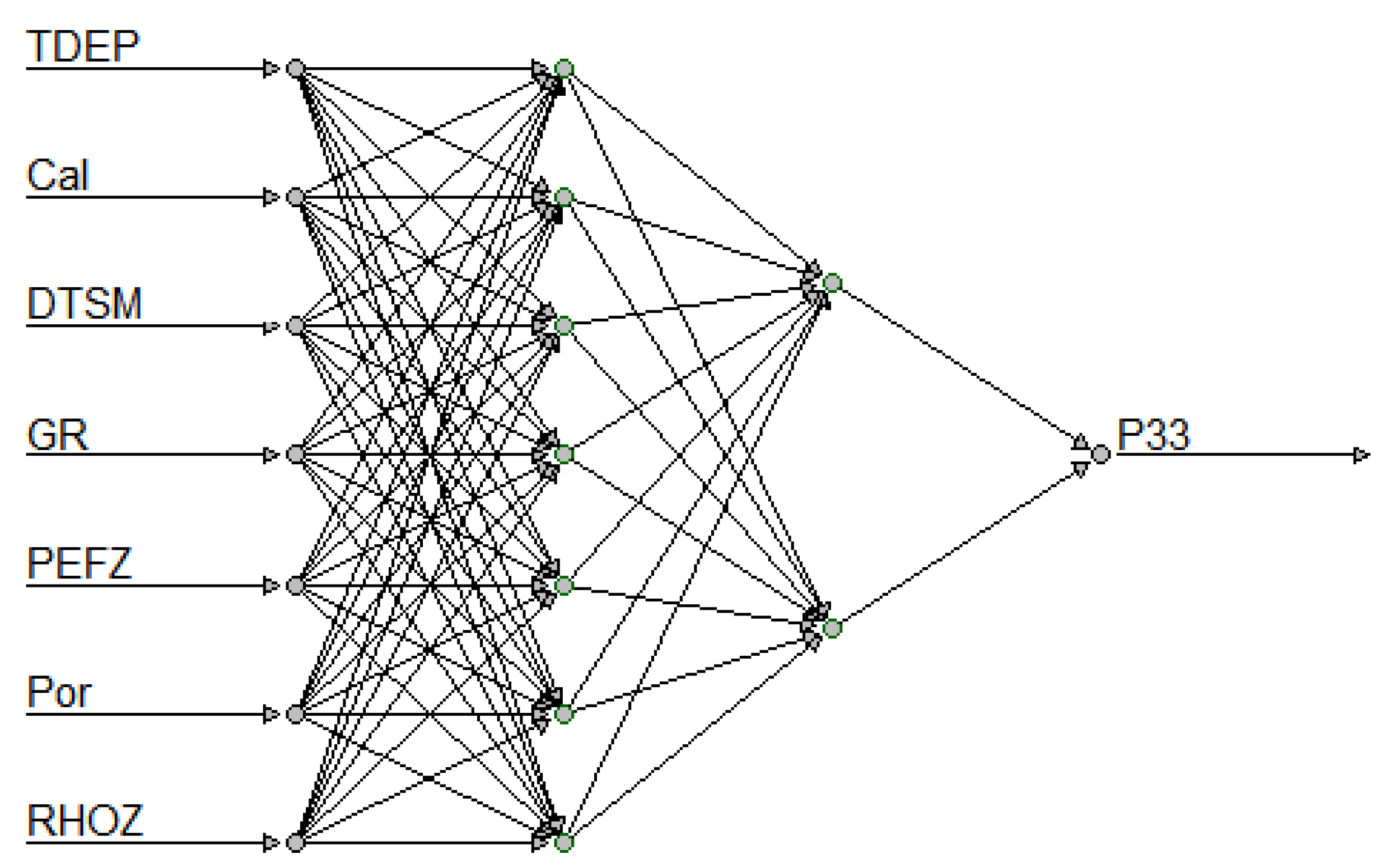
The initial approach involves utilizing the pure ANN model, which comprises two hidden layers and 7, 2 nodes, to forecast the fracture porosity (P33) in each layer, as illustrated in Figure 8. To accomplish this, the dataset is split into randomly two distinct parts, with the training data comprising 80% of the dataset and the test data 20%. The training data is utilized to train the ANN model, and the accuracy of the model is evaluated based on the metrics testing it on the test data. The objective function we used to train the data and validation is the Roor Mean Squared Error (RMSE). This approach offers the advantage of balancing the contribution of errors from the entire range of fracture porosity values.
Where n is the total number of observations and is the actual data and is the data predicted using a machine learning algorithm. This approach is implemented to assess the performance of the ANN model and to determine its suitability for the forecasting of P33.
Figure 8.
ANN model architecture
Hybrid Model Support vector machines- Artificial neural network (SVM-ANN)
Support vector machine (SVM) is a type of supervised learning method that can separate data into two classes [31]. Its basic model is a linear classifier that defines a decision boundary with the largest spacing in the feature space [31]. SVM differs from other linear classifiers in that it maximizes the spacing or margin between the decision boundary and the closest data points. By using kernel tricks, SVM can also classify nonlinear data by transforming it into a higher-dimensional space where a linear boundary may be found. The learning strategy of SVM involves solving a convex quadratic programming problem to maximize the margin. Overall, SVM is considered the optimal algorithm for solving convex quadratic programming problems in supervised learning tasks [2].
The second approach employed in this project utilizes both Support Vector Machine (SVM) and Artificial Neural Network (ANN) algorithms. The SVM algorithm determines the presence of fractures in formations by classifying the P33 variable into two categories: values of zero and greater than zero. An observed P33 value of zero indicates an unfractured portion of the formation, while a value greater than zero indicates the presence of fractures. Similar to the previous method, the dataset is randomly partitioned into two groups, namely the training data and the test data. The SVM model is initially trained using the training data to distinguish between P33 values of zero and non-zero. At the same time, all datasets with a P33 value of zero are excluded from the training data. Subsequently, the ANN model is trained exclusively using data from fractured formations. Finally, the accuracy of both models is evaluated using the test data (Figure 9).
The ANN model used for the second approach (hybrid) has an architecture of two hidden layers and 10, 10 nodes on each layer, as shown in Figure 10
3. Results and Discussion
The pair plots are generated using R and presented in Figure 11. The correlation plot indicates that the "DTCO_Final" exhibits the weakest correlation with the P33, which represents the porosity of fractures. However, a nearly linear relationship is observed between the "DTCO" and the "DTSM". Thus, when training the ANN and SVM-ANN models, the factor "DTCO" is removed from the model training. It can also be observed that P33 has a good correlation with the bulk density (RHOZ) and photoelectric factor (PEFZ).
As mentioned earlier, the data consists of 5008 samples, and they were randomly allocated into two groups. The first set contains 80% of the total samples, referred to as the "training data subset" used to train machine learning algorithms. The remaining 20%, known as the ’test data subset,’ were utilized to evaluate the efficacy of the machine learning methods. The error metric Root Mean Square Error (RMSE) was chosen to quantify the efficiency of the models.
The accurate estimation of fracture porosity is essential as it plays a vital role in the assessment of hydrocarbon reserves. Machine learning (ML) algorithms have been increasingly employed in fracture porosity estimation due to their ability to handle large volumes of data and identify complex patterns. In this regard, two ML algorithms, pure Artificial Neural Networks and the hybrid SVM-ANN model, have been evaluated in terms of their effectiveness in estimating fracture porosity. This study aimed to provide insights into the comparative performance of these two ML algorithms and highlighted the potential of hybridized machine learning algorithms in fracture porosity estimation.
3.1. Artificial Neural Network (ANN)
We systematically investigated to find out the optimum number of hidden layers and the number of neurons in each layer required for the ANN model. Further, we observed the response of the objective function to determine the best network structure for our implementation of the neural network approach. We observed that increasing the number of layers and neurons increases the score of the objective function, but that is because of overfitting. Overfitting happens when a model is too complex and goes beyond the task of accurately fitting the patterns in the data, leading to it memorizing the training points. This causes the model’s performance to improve continuously on the training dataset, but this improvement comes at the cost of the model’s ability to generalize to new, unseen data [32]. Due to noise in the training data and its potential inability to fully represent the entire population, it is crucial to prevent overfitting by carefully selecting the appropriate size for the neural network. The optimum ANN model consisted of two layers with a number of neurons 7 and 2 in each layer. The ANN is implemented on R with the algorithm backpropagation with weight backtracking and the highest learning rate of 0.01.
The P33 predictions of the ANN are presented in the Figure 12. The validity of the ANN is checked on the separate data that was not used during the training. We used root mean squared error (RMSE) to measure the performance and validity of the machine learning methods. We found the RMSE values of 4.13e-5 and 20e-5 for the well-A and well-B, respectively.
The present study showcases the results obtained from our analysis, where we employed an Artificial Neural Network (ANN) to predict fracture porosity based on the provided input logs. The predicted values, alongside the corresponding input logs, are depicted in Figure 13 and Figure 14. Upon examination, it becomes evident that the ANN predictions exhibit a discernible correlation with the observed trend of actual fracture porosity. Particularly noteworthy is the notable accuracy of the ANN predictions when the P33 parameter attains relatively high values.
To gain a more comprehensive understanding, we extended the reference depth scale for the results obtained from well-A and well B, as depicted in Figure 15 and Figure 16, respectively. Upon closer inspection, it becomes apparent that the accuracy of the ANN predictions is not entirely flawless compared to the actual values. Although the overall trend of the predicted fracture porosity closely aligns with the observed data, certain discrepancies arise, especially within the lower range of fracture porosities, specifically within the depth interval highlighted in a circle as ’X’ (Figure 13). During this range, the ANN tends to overestimate the fracture porosities, thereby incorrectly suggesting the presence of fractures where there are none.
Consequently, this discrepancy was a primary motivation for our search for alternative machine learning algorithms and eventually led us to adopt a hybrid ML approach. By leveraging a hybrid ML framework, we aim to refine the accuracy of fracture porosity predictions, specifically targeting intervals where actual fracture porosity is absent but erroneously estimated by the ANN. The results of the hybrid approach are presented in the following section.
3.2. Support Vector Machines – Artificial Neural Network (SVM-ANN)
In the preceding section, we established that the Artificial Neural Network (ANN) yielded higher P33 values in nonfractured layers. In order to address this issue, we adopted a two-step approach. Firstly, we employed the Support Vector Machine (SVM) algorithm to classify the depth interval into fractured and nonfractured layers. We utilized a radial basis kernel with the SVM algorithm to accomplish this. Following the classification, we proceeded to validate the predictions on test data. Subsequently, we exclusively utilized data from the fractured layers to predict P33 using the ANN. Our objective was to avoid overfitting the ANN model, as was emphasized in the previous section.
To determine the optimal configuration for our analysis, we conducted a systematic investigation of the number of layers and neurons in the ANN. Through this exploration, we discovered that employing two hidden layers, each consisting of 10 neurons, yielded the most favorable results. We applied the ANN algorithm that utilizes backpropagation with weight backtracking, similar to the previous case.
By incorporating the SVM algorithm for layer classification and carefully fine-tuning the ANN model, we aimed to enhance the accuracy of our predictions and mitigate the biases observed in nonfractured layers. This approach allowed us to overcome the challenges posed by the initial ANN predictions and enabled more reliable estimations of P33 values in the fractured layers.
The cross-validation on the testing data of wells-A and-B is presented in Figure 17. It can be seen that the R2 score and the RMSE errors are superior to that of ANN predictions.
As elaborated upon in the preceding section, the precision of the error estimates is expressed in terms of the Root Mean Square Error (RMSE) and is tabulated in Table 2.
The table compares the root mean square error (RMSE) values of two different models: Pure ANN and Hybrid Model. The RMSE measures the average difference between predicted and actual values, with lower values indicating better performance.For Well-A, the Pure ANN model has an RMSE of 0.092, while the Hybrid Model achieves a lower RMSE of 0.083. This suggests that the Hybrid Model outperforms the Pure ANN model in predicting values for Well-A, as it has a smaller error. Similarly, for Well-B, the Pure ANN model has an RMSE of 0.145, whereas the Hybrid Model achieves a lower RMSE of 0.114. Once again, the Hybrid Model shows improved performance compared to the Pure ANN model for predicting values related to Well-B. In summary, the table highlights that the Hybrid Model performs better than the Pure ANN model in terms of RMSE for both Well-A and Well-B, indicating its superiority in predicting values for these wells.
The results are presented in different scales, specifically 1:2000 scale for Figure 13 and Figure 14, and 1:240 scale for Figure 15 and Figure 16. Figure 13 and Figure 14 illustrate that there is a similarity in the overall trend between the predicted fractural porosities and the actual fractural porosities. This means that the SVM-ANN models are able to capture the general patterns and variations in the porosity values. Figure 15 and Figure 16 provide more detailed information. The sections highlighted with ’A’ in these Figure 15 and Figure 16 indicate that the artificial neural network (ANN) underpredicts the P33 values while the SVM-ANN model tends to make more accurate porosity predictions. This suggests that the SVM-ANN model performs better than the ANN model in this particular aspect.
However, there is a layer marked with ’B’ in Figure 16 where neither the ANN nor the SVM-ANN models are able to predict the actual P33 values accurately. This could be an attempt to avoid overfitting the data. Overfitting occurs when a model becomes too complex and starts fitting the noise or peculiarities of the training data instead of capturing the underlying patterns. We observe that the surrounding zones, which have similar log signatures, do not exhibit high fracture porosity. Therefore, the models intentionally avoid making predictions that incorrectly identify these zones as having high porosity.
Conclusions
This study employs an integrative approach to assess the fracture porosity in a tight gas naturally fractured reservoir, Ahnet field, Algeria and conducts a comparative analysis using machine learning techniques to predict the fracture porosity. The results lead to the following conclusions:
- The results from the Image logs and the Sonic scanner integration show that the porosity of fractures can be estimated accurately.
- One of the objectives of the present study is to select an appropriate machine learning model to predict fracture porosity. The results demonstrate that SVM-ANN outperforms ANN in predicting fracture porosity.
- The data used in this study were obtained from only two wells in the heterogeneous and giant field. Thus, the applicability of these samples to the entire field is debatable. Furthermore, due to the limited sample size of only two wells from the Ahnet field, constructing the most precise predictive machine learning models is challenging in this study. Furthermore, the approach adopted in this study prioritized cost efficiency while maintaining accuracy in fracture porosity estimations.
- By neglecting the potential insights that could be gained from incorporating core data, which can be expensive and time-consuming to acquire, this approach may limit the accuracy of the predictions. It is worth noting that core data can provide essential information on rock properties and fluid behavior.
- Future research efforts should consider the potential benefits of incorporating more well logs, and image logs data in fracture porosity estimations and explores ways to minimize the associated costs and time requirements. Therefore, using a higher number of samples is highly recommended to enhance the prediction capabilities of the model.
- This research article demonstrated that the SVM-ANN-based model provides accurate fracture porosity estimations and can serve as a replacement in the absence of costly core datasets.
Author Contributions
Conceptualization, data curation, and original draft preparation, G.I. and D.I.; methodology and validation, P.P; Validation, Investigation and Visualization, R.N.; review and editing, S.E.
Conflicts of Interest
The authors declare no conflict of interest
References
- Gutmanis, J.C. Basement Reservoirs – A Review of Their Geological and Production Characteristics. In Proceedings of the IPTC 2009: International Petroleum Technology Conference; European Association of Geoscientists & Engineers; 2009. [Google Scholar]
- John, B. Curtis1 Fractured Shale-Gas Systems. Am. Assoc. Pet. Geol. Bull. 2002, 86, 1921–1938. [Google Scholar] [CrossRef]
- Sulak, R.M. Ekofisk Field. The First 20 Years. JPT, J. Pet. Technol. 1991, 43, 1265–1271. [Google Scholar] [CrossRef]
- Kharrat, R. A Comprehensive Review of Fracture Characterization and Its. 2023.
- Ameen, M.S.; MacPherson, K.; Al-Marhoon, M.I.; Rahim, Z. Diverse Fracture Properties and Their Impact on Performance in Conventional and Tight-Gas Reservoirs, Saudi Arabia: The Unayzah, South Haradh Case Study. Am. Assoc. Pet. Geol. Bull. 2012, 96, 459–492. [Google Scholar] [CrossRef]
- Mahmood, M.N.; Guo, B. An Analytical Method for Optimizing Fracture Spacing in Shale Oil Reservoirs. In Proceedings of the SPE Liquids-Rich Basins Conference-North America; OnePetro; 2019. [Google Scholar]
- Laubach, S.; Marrett, R.; Olson, J. New Directions in Fracture Characterization. Lead. Edge 2000, 19, 704–711. [Google Scholar] [CrossRef]
- Clarkson, C.R.; Haghshenas, B.; Ghanizadeh, A.; Qanbari, F.; Williams-Kovacs, J.D.; Riazi, N.; Debuhr, C.; Deglint, H.J. Nanopores to Megafractures: Current Challenges and Methods for Shale Gas Reservoir and Hydraulic Fracture Characterization. J. Nat. Gas Sci. Eng. 2016, 31, 612–657. [Google Scholar] [CrossRef]
- Suhag, A.; Ranjith, R.; Aminzadeh, F. Comparison of Shale Oil Production Forecasting Using Empirical Methods and Artificial Neural Networks. In Proceedings of the Day 3 Wed, October 11, 2017, SPE, October 11 2017. [Google Scholar]
- Choubey, S.; Karmakar, G.P. Artificial Intelligence Techniques and Their Application in Oil and Gas Industry. Artif. Intell. Rev. 2021, 54, 3665–3683. [Google Scholar] [CrossRef]
- Rahmanifard, H.; Plaksina, T. Application of Artificial Intelligence Techniques in the Petroleum Industry: A Review. Artif. Intell. Rev. 2019, 52, 2295–2318. [Google Scholar] [CrossRef]
- Misra, S.; Li, H. Noninvasive Fracture Characterization Based on the Classification of Sonic Wave Travel Times. In Machine Learning for Subsurface Characterization; Elsevier, 2020; pp. 243–287.
- Alipour, M.; Esatyana, E.; Sakhaee-Pour, A.; Sadooni, F.N.; Al-Kuwari, H.A. Characterizing Fracture Toughness Using Machine Learning. J. Pet. Sci. Eng. 2021, 200, 108202. [Google Scholar] [CrossRef]
- Zheng, Y.; Li, J.; Lin, R.; Hu, H.; Gao, K.; Huang, L.; Sciences, A.; Alamos, L. Physics-Guided Machine Learning Approach to Characterizing Small-Scale Fractures in Geothermal Fields. PROCEEDINGS, 46th Work. Geotherm. Reserv. Eng. 2021, 1–9. [Google Scholar]
- Singh, A.; Rabbani, A.; Regenauer-Lieb, K.; Armstrong, R.T.; Mostaghimi, P. Computer Vision and Unsupervised Machine Learning for Pore-Scale Structural Analysis of Fractured Porous Media. Adv. Water Resour. 2021, 147, 103801. [Google Scholar] [CrossRef]
- Boudjema, A. Évolution Structurale Du Bassin Pétrolier" Triasique" Du Sahara Nord Oriental (Algérie), Paris 11, 1987.
- Klitzsch, E.; Gray, C. The Structural Development of Parts of North Africa since Cambrian Time. In Proceedings of the Symposium on the geology of Libya: Tripoli, Faculty of Sciences, University of Libya; 1971; pp. 256–260. [Google Scholar]
- Beuf, S. GRES DU PALEOZOIQUE INFERIEUR AU SAHARA; editions Technip, 1971. 1971.
- Robertson, A.H.F.; Dixon, J.E. Introduction: Aspects of the Geological Evolution of the Eastern Mediterranean. Geol. Soc. London, Spec. Publ. 1984, 17, 1–74. [Google Scholar]
- Guiraud, R.; Maurin, J.-C. Early Cretaceous Rifts of Western and Central Africa: An Overview. Tectonophysics 1992, 213, 153–168. [Google Scholar] [CrossRef]
- Allaoui, A.; Belksier, M.S.; Ameur-Zaimeche, O.; Kechiched, R.; Remita, A.; Fellah, L.; Lamouri, B.; Habes, S. The Lower Silurian Black Shales from the Ahnet Basin (S.W. Algerian Saharan Platform): A Comprehensive Mineralogical Study and Paleoenvironmental Implications. Arab. J. Geosci. 2022, 15, 1103. [Google Scholar] [CrossRef]
- Sonatrach Internal Report.
- Lander, L.A.; Silva, A.; Chiquito, J.; Cadena, A. Improved Fracture Characterization in the La Paz Field: A Case Study. In Proceedings of the SPE Latin American and Caribbean Petroleum Engineering Conference; OnePetro; 2015. [Google Scholar]
- Maeso, C.; Dubourg, I.; Quesada, D.; ElNour, W.A. Uncertainties in Fracture Apertures Calculated from Electrical Borehole Images. In Proceedings of the International Petroleum Technology Conference; OnePetro; 2015. [Google Scholar]
- Li, H. Statistical Learning Methods. Tsinghua Univ. Press 2012, 95–115. [Google Scholar]
- Huang, Z.; Shimeld, J.; Williamson, M.; Katsube, J. Permeability Prediction with Artificial Neural Network Modeling in the Venture Gas Field, Offshore Eastern Canada. Geophysics 1996, 61, 422–436. [Google Scholar] [CrossRef]
- Tariq, Z.; Elkatatny, S.M.; Mahmoud, M.A.; Abdulraheem, A.; Abdelwahab, A.Z.; Woldeamanuel, M. Estimation of Rock Mechanical Parameters Using Artificial Intelligence Tools. In Proceedings of the 51st U.S. Rock Mechanics/Geomechanics Symposium; OnePetro; 2017. [Google Scholar]
- Agatonovic-Kustrin, S.; Beresford, R. Basic Concepts of Artificial Neural Network (ANN) Modeling and Its Application in Pharmaceutical Research. J. Pharm. Biomed. Anal. 2000, 22, 717–727. [Google Scholar] [CrossRef] [PubMed]
- Ebrahimi, A.; Izadpanahi, A.; Ebrahimi, P.; Ranjbar, A. Estimation of Shear Wave Velocity in an Iranian Oil Reservoir Using Machine Learning Methods. J. Pet. Sci. Eng. 2022, 209, 109841. [Google Scholar] [CrossRef]
- Wang, P.; Peng, S. On a New Method of Estimating Shear Wave Velocity from Conventional Well Logs. J. Pet. Sci. Eng. 2019, 180, 105–123. [Google Scholar] [CrossRef]
- Suthaharan, S.; Suthaharan, S. Support Vector Machine. Mach. Learn. Model. algorithms big data Classif. Think. with examples Eff. Learn. 2016, 207–235. [Google Scholar]
- Ying, X. An Overview of Overfitting and Its Solutions. J. Phys. Conf. Ser. 2019, 1168, 022022. [Google Scholar] [CrossRef]
Figure 1.
Location of the Area of study [21]
Figure 1.
Location of the Area of study [21]
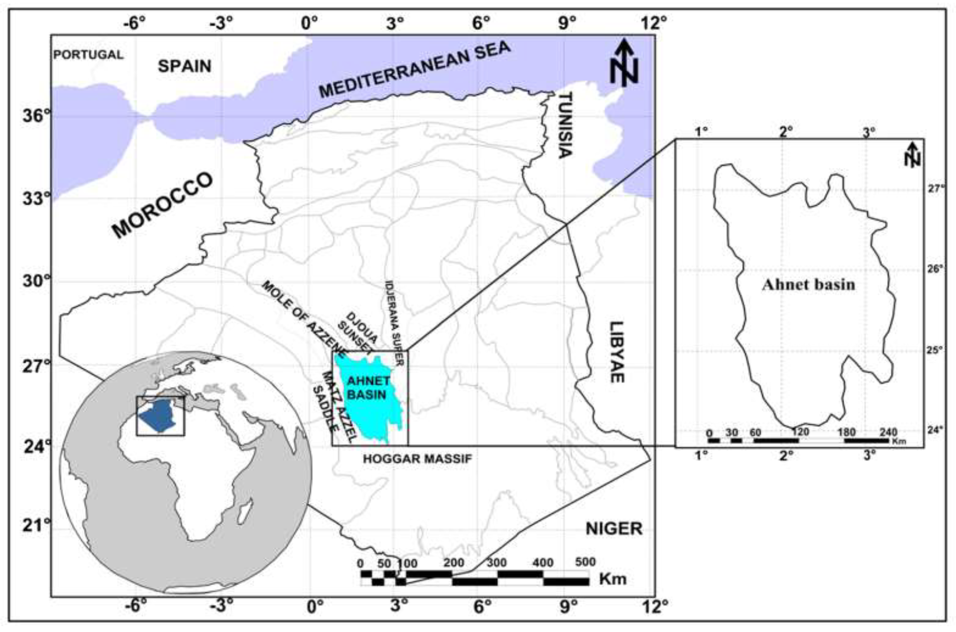
Figure 2.
Lithostratigraphic column of the Cambro-Ordovician formations in the Ahnet Basin , modified after [22].
Figure 2.
Lithostratigraphic column of the Cambro-Ordovician formations in the Ahnet Basin , modified after [22].
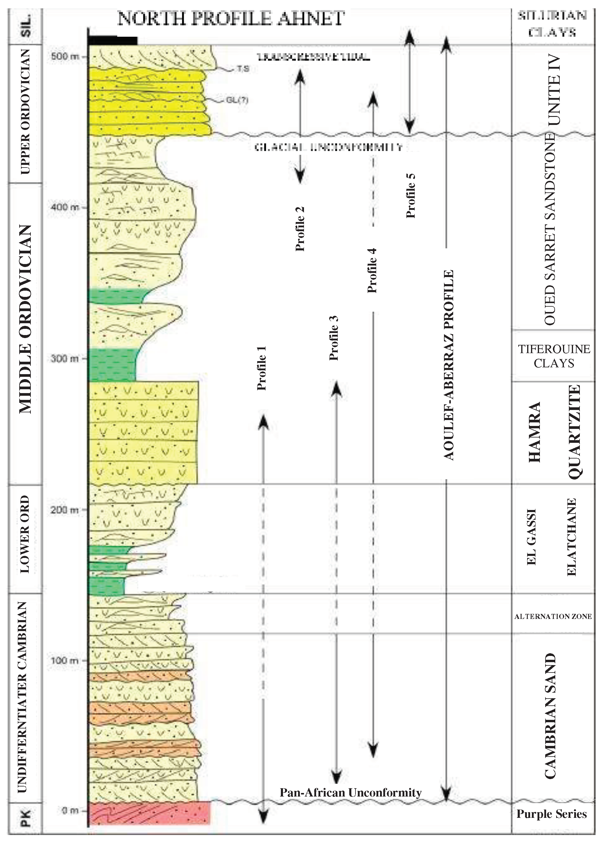
Figure 3.
The proposed workflow for the fracture porosity estimation.
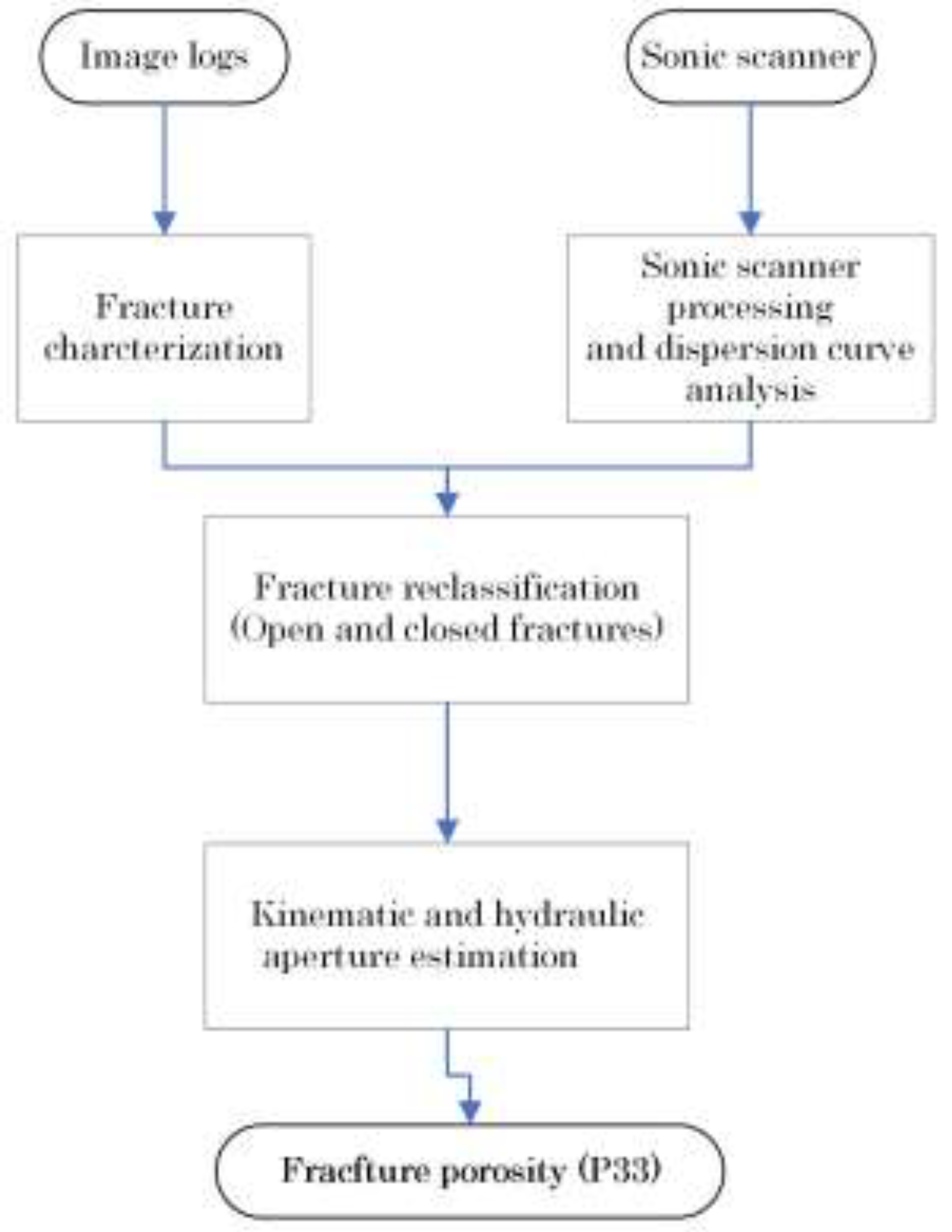
Figure 4.
Fractures reclassification process using dispersion analysis plots.
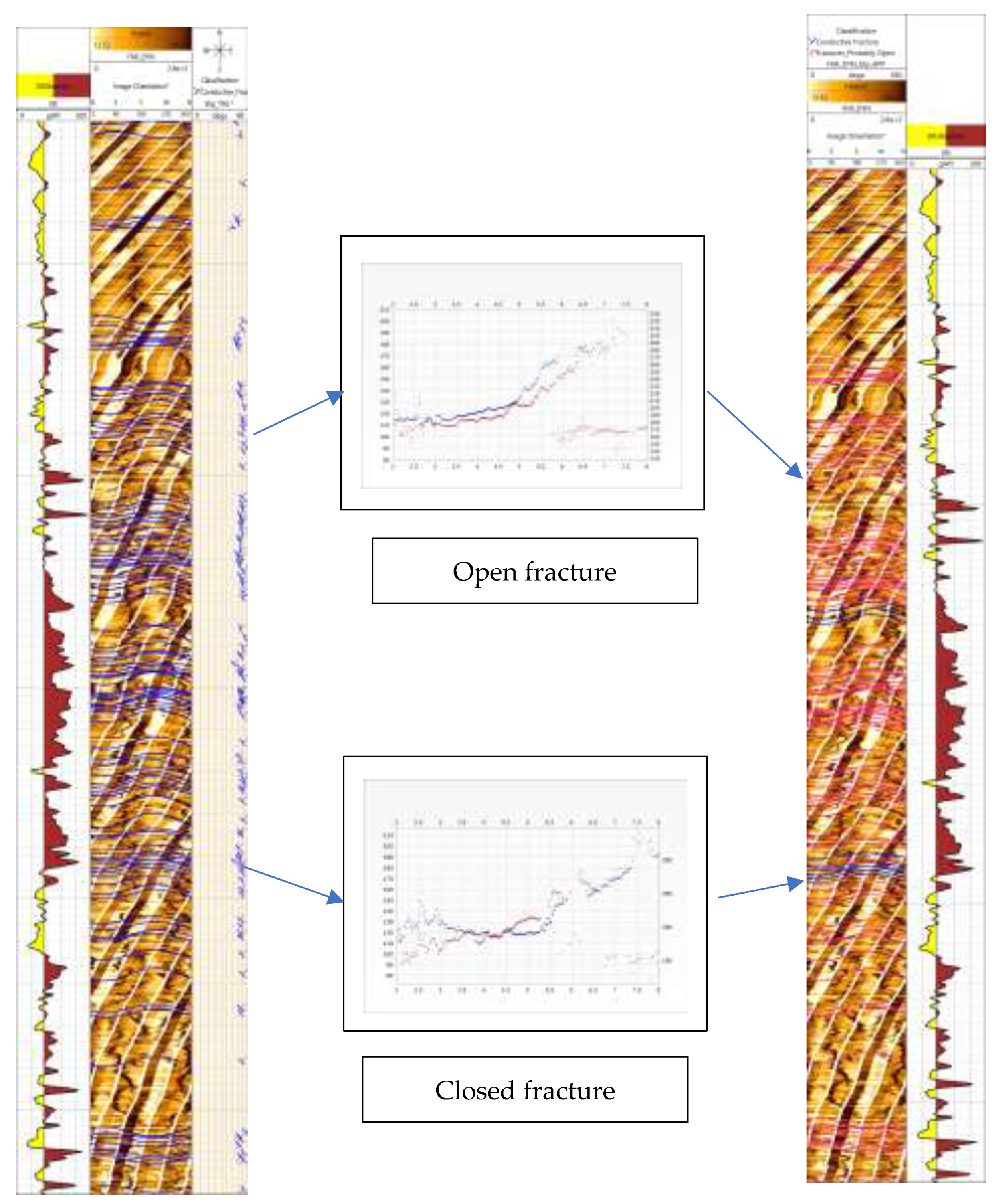
Figure 5.
Various rock characteristics as displayed in a typical borehole through the Cambro-Ordovician formation. Track 1: Gamma Ray (G.R.), Track 2: Dynamic Image log (FMI_DYN) with open fracture sines, Track 3 Fracture tadpoles (dip and azimuth), Track 4: Fracture aperture along the facture sine wave, Track 5: Mean fracture kinematic (FVA) and hydraulic aperture.
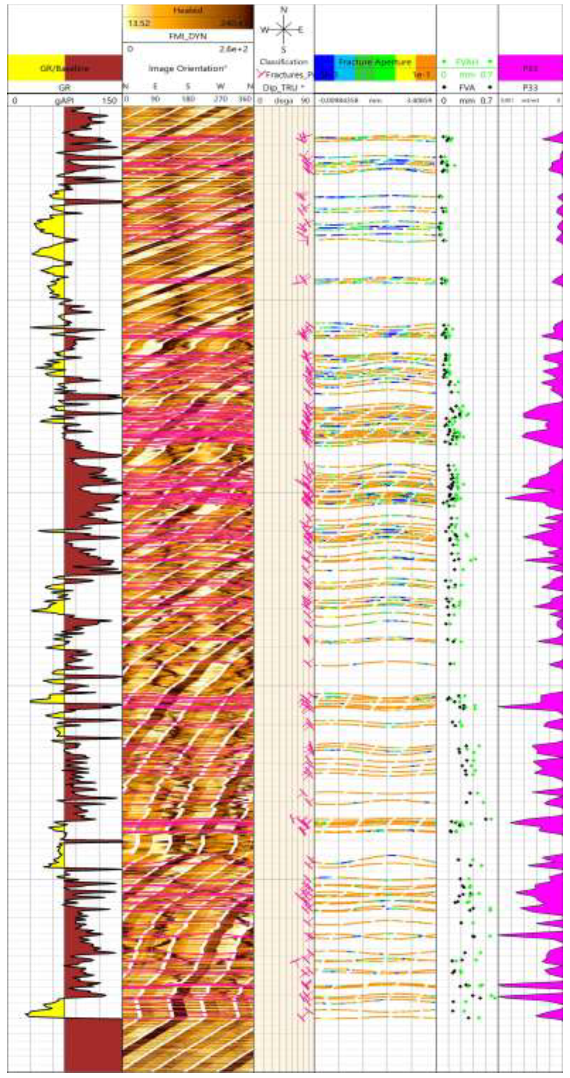
Figure 6.
Data distribution of each input log and the P33. The corresponding statistical information and the units of each variable is provided in the Table 1.
Figure 6.
Data distribution of each input log and the P33. The corresponding statistical information and the units of each variable is provided in the Table 1.
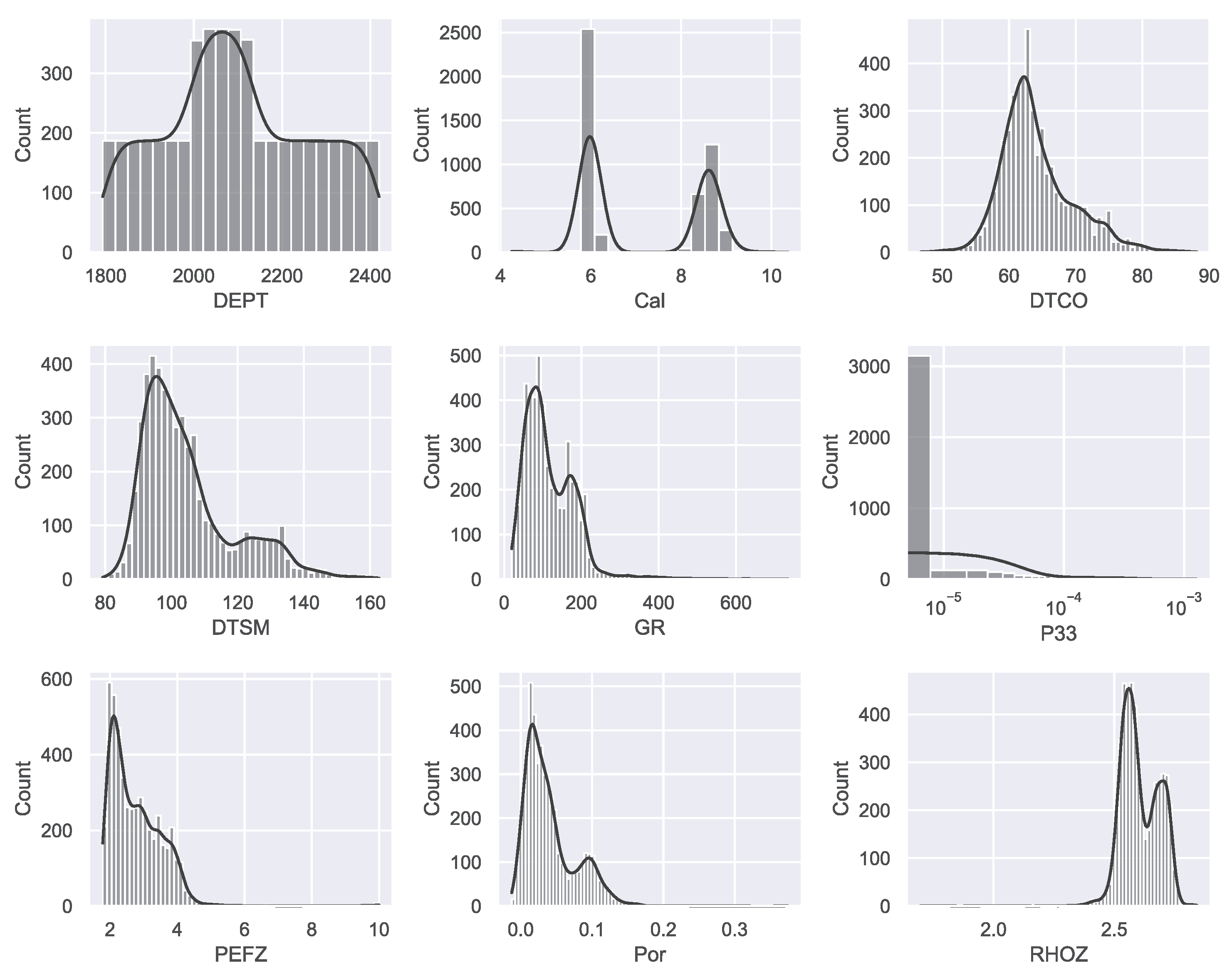
Figure 7.
Input logs used for the fracture porosity prediction (well-B), Track 1: Gamma-ray (G.R.) and caliper (Cal), Track 2: Shear (DTSM) and compressional (DTCO) slowness, Track 3 Photo Electric Factor (PEF), Bulk density (RHOZ), and Neutron porosity (Por).
Figure 7.
Input logs used for the fracture porosity prediction (well-B), Track 1: Gamma-ray (G.R.) and caliper (Cal), Track 2: Shear (DTSM) and compressional (DTCO) slowness, Track 3 Photo Electric Factor (PEF), Bulk density (RHOZ), and Neutron porosity (Por).
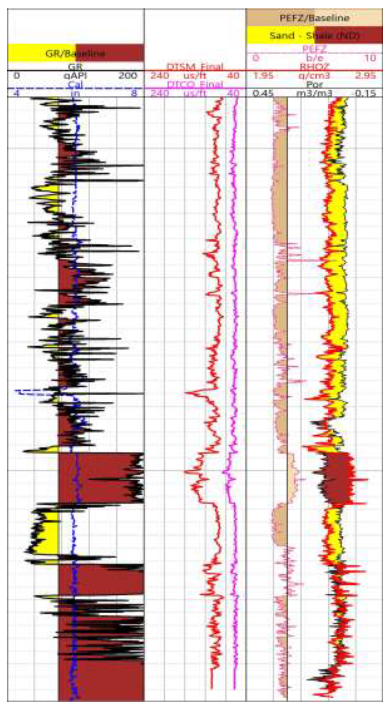
Figure 9.
Flowchart for the hybrid model
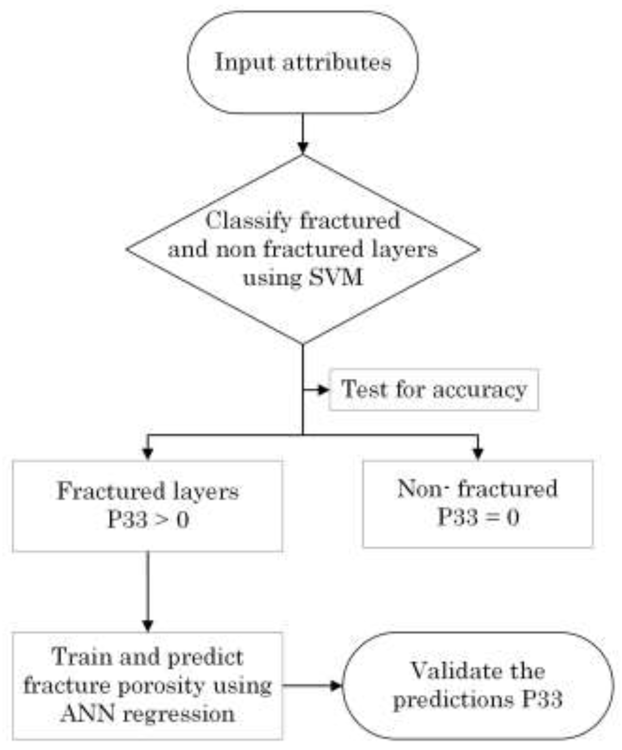
Figure 10.
ANN model used for the hybrid approach
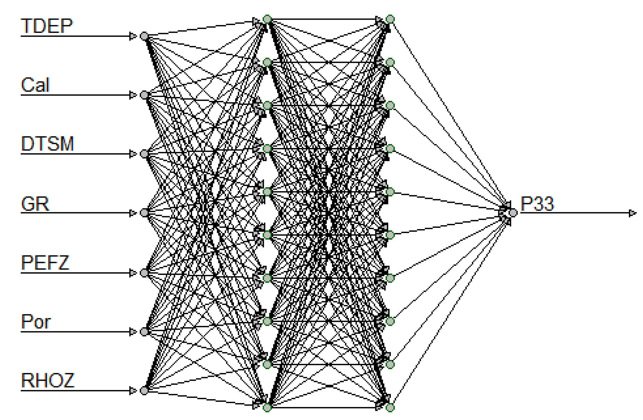
Figure 11.
Pair plots of the input attributes and P33 data.
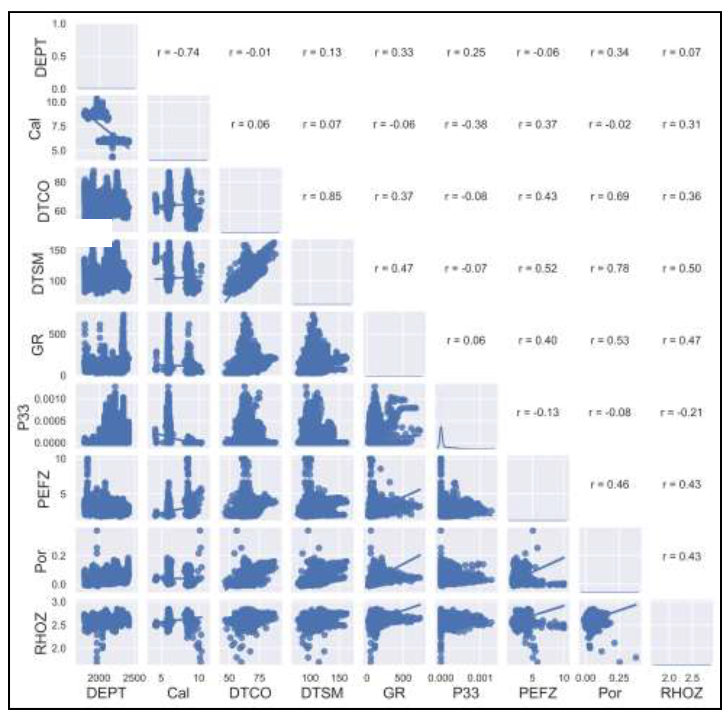
Figure 12.
Crosplots of predicted data and the actual data used in the cross-validation using the ANN model.
Figure 12.
Crosplots of predicted data and the actual data used in the cross-validation using the ANN model.
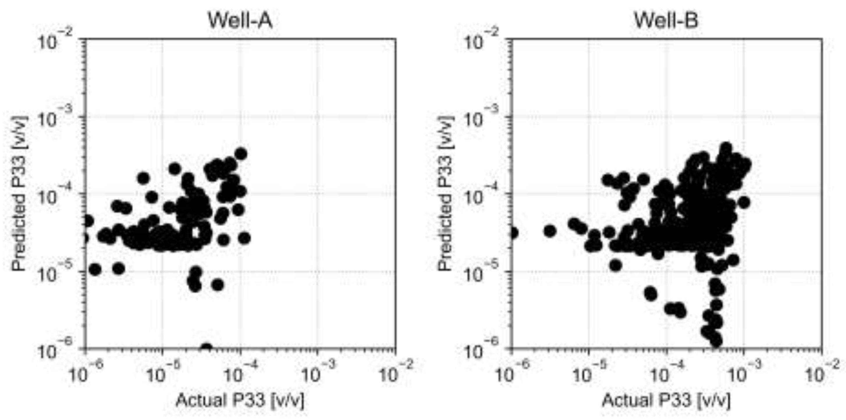
Figure 13.
Well-A presented at the depth reference scale 1:2000 m. Track-I: Depth, Track-II: Caliper and Gamma Ray, Track-III: Compressional and Shear slowness, Track-IV Neutron porosity, Bulk density and photoelectric factor and Track-V: Actual P33 porosity, ANN predicted porosity and SVM-ANN predicted porosity.
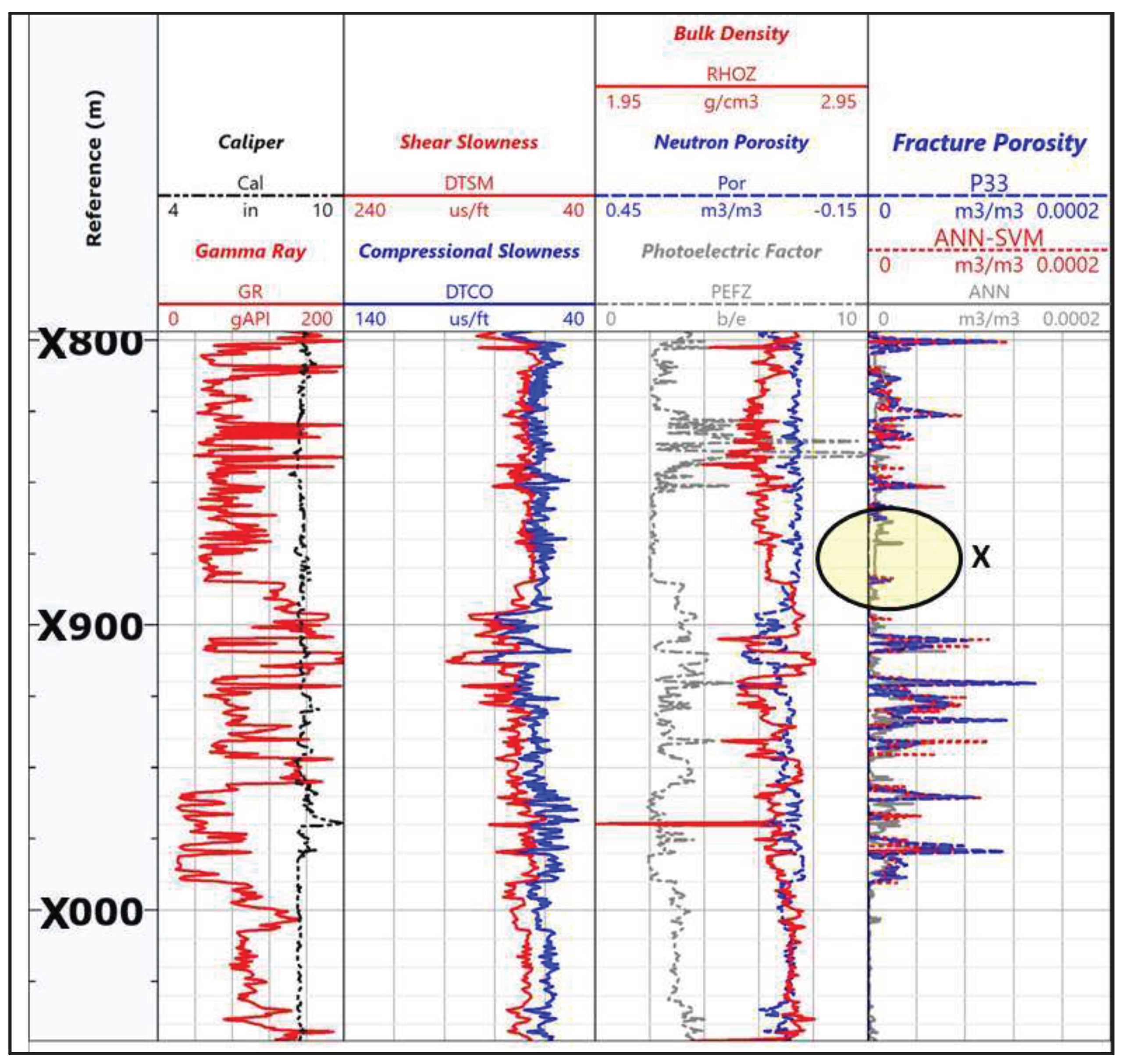
Figure 14.
Figure 14. Well-B presented at the depth reference scale 1:2000 m. Track-I: Depth, Track-II: Caliper and Gamma Ray, Track-III: Compressional and Shear slowness, Track-IV Neutron porosity, Bulk density and photoelectric factor and Track-V: Actual P33 porosity, ANN predicted porosity and SVM-ANN predicted porosity.
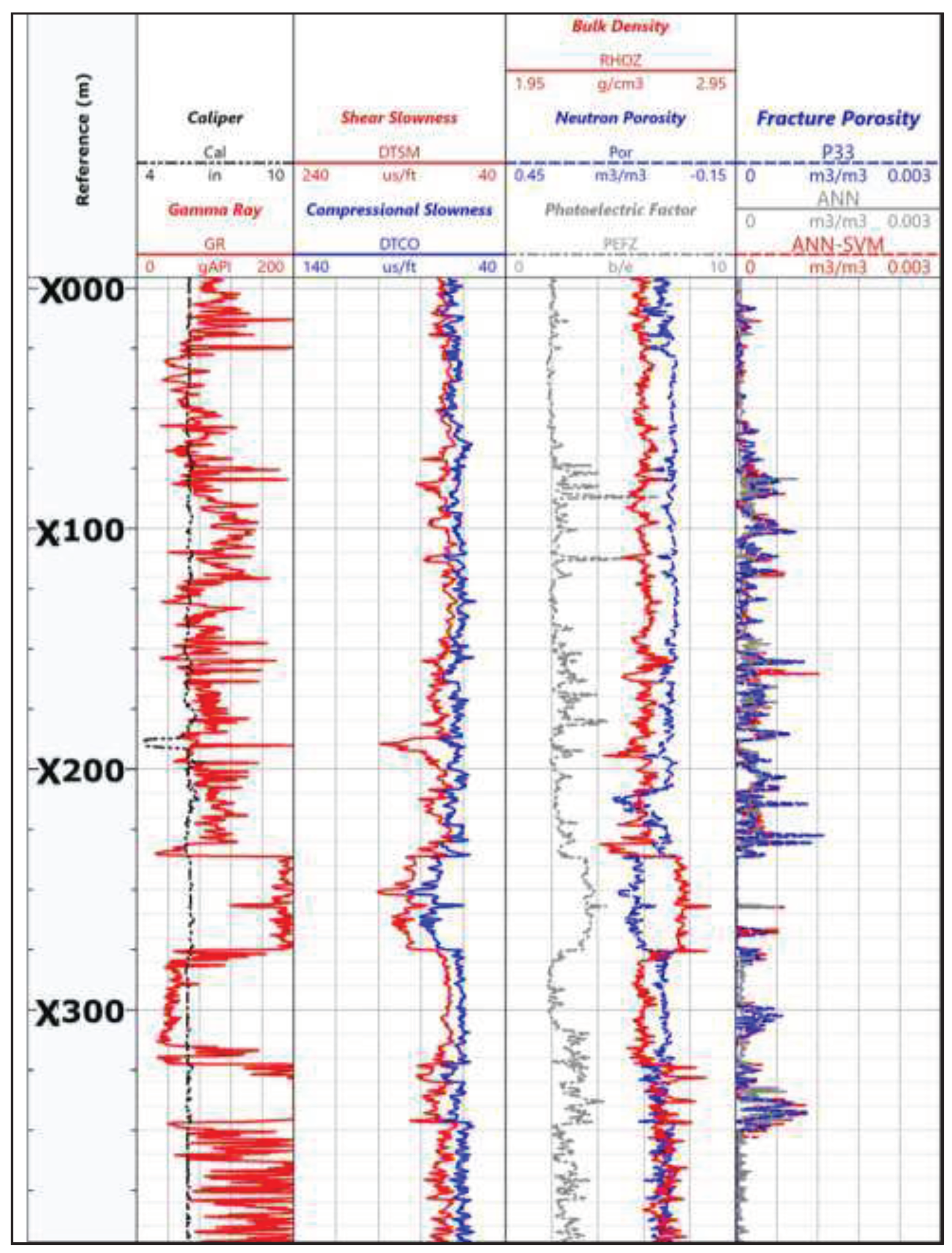
Figure 15.
Well-A presented at the depth reference scale 1:240 m. Track-I: Depth, Track-II: Caliper and Gamma Ray, Track-III: Compressional and Shear slowness, Track-IV Neutron porosity, Bulk density and photoelectric factor and Track-V: Actual P33 porosity, ANN predicted porosity and SVM-ANN predicted porosity.
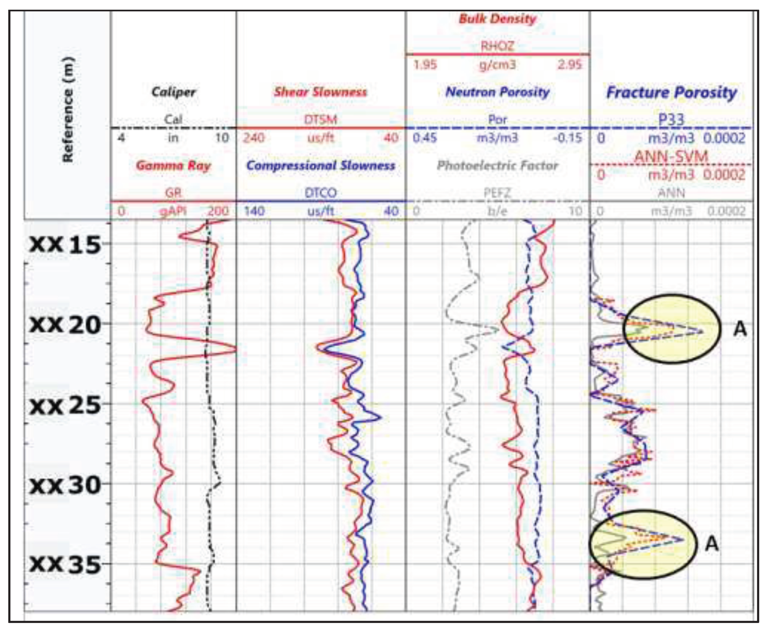
Figure 16.
Well-B presented at the depth reference scale 1:240 m: Track-I: Depth, Track-II: Caliper and Gamma Ray, Track-III: Compressional and Shear slowness, Track-IV Neutron porosity, Bulk density and photoelectric factor and Track-V: Actual P33 porosity, ANN predicted porosity and SVM-ANN predicted poros
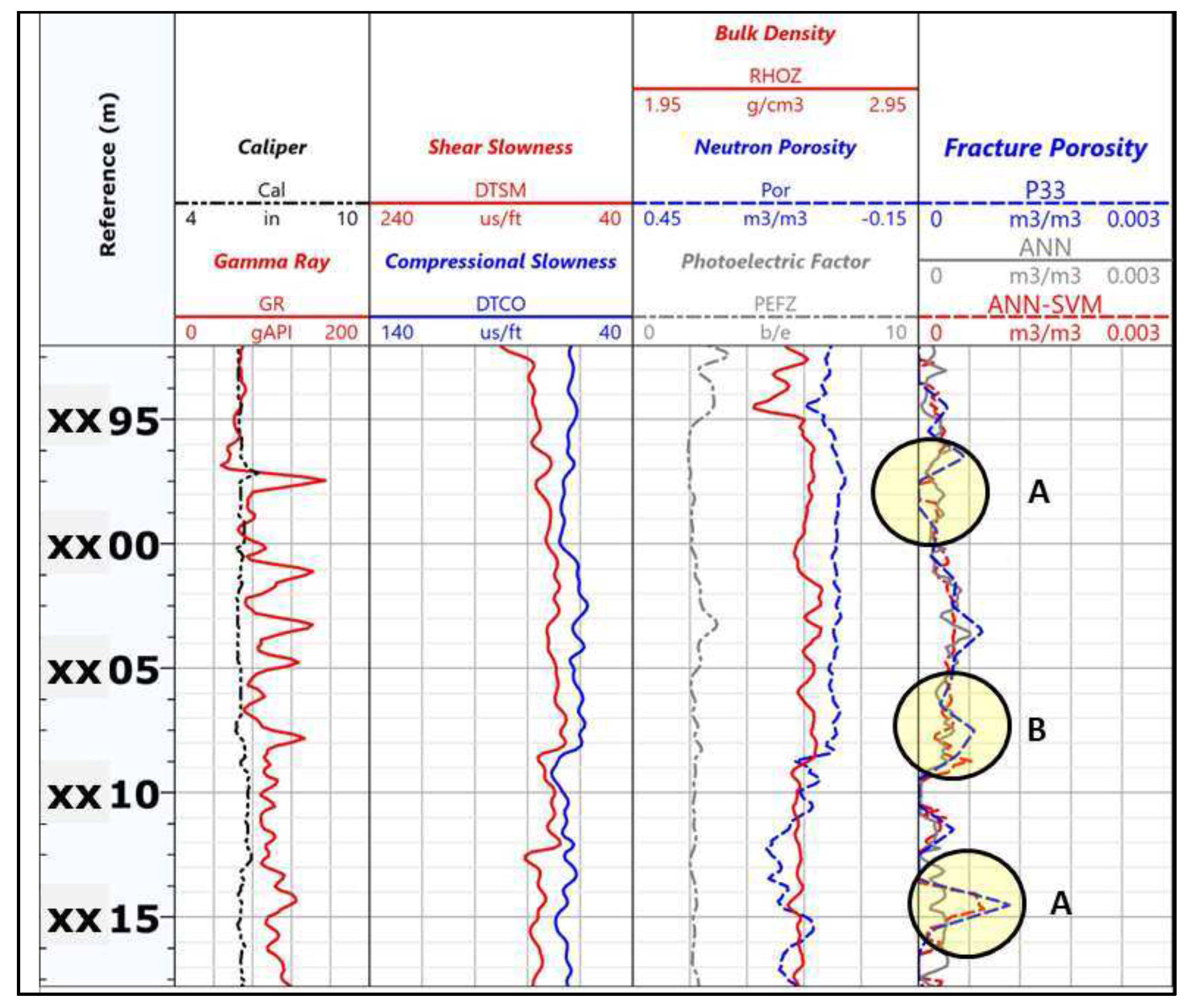
Figure 17.
Crosplots of predicted data and the actual data used in the cross-validation using the SVM-ANN model.
Figure 17.
Crosplots of predicted data and the actual data used in the cross-validation using the SVM-ANN model.
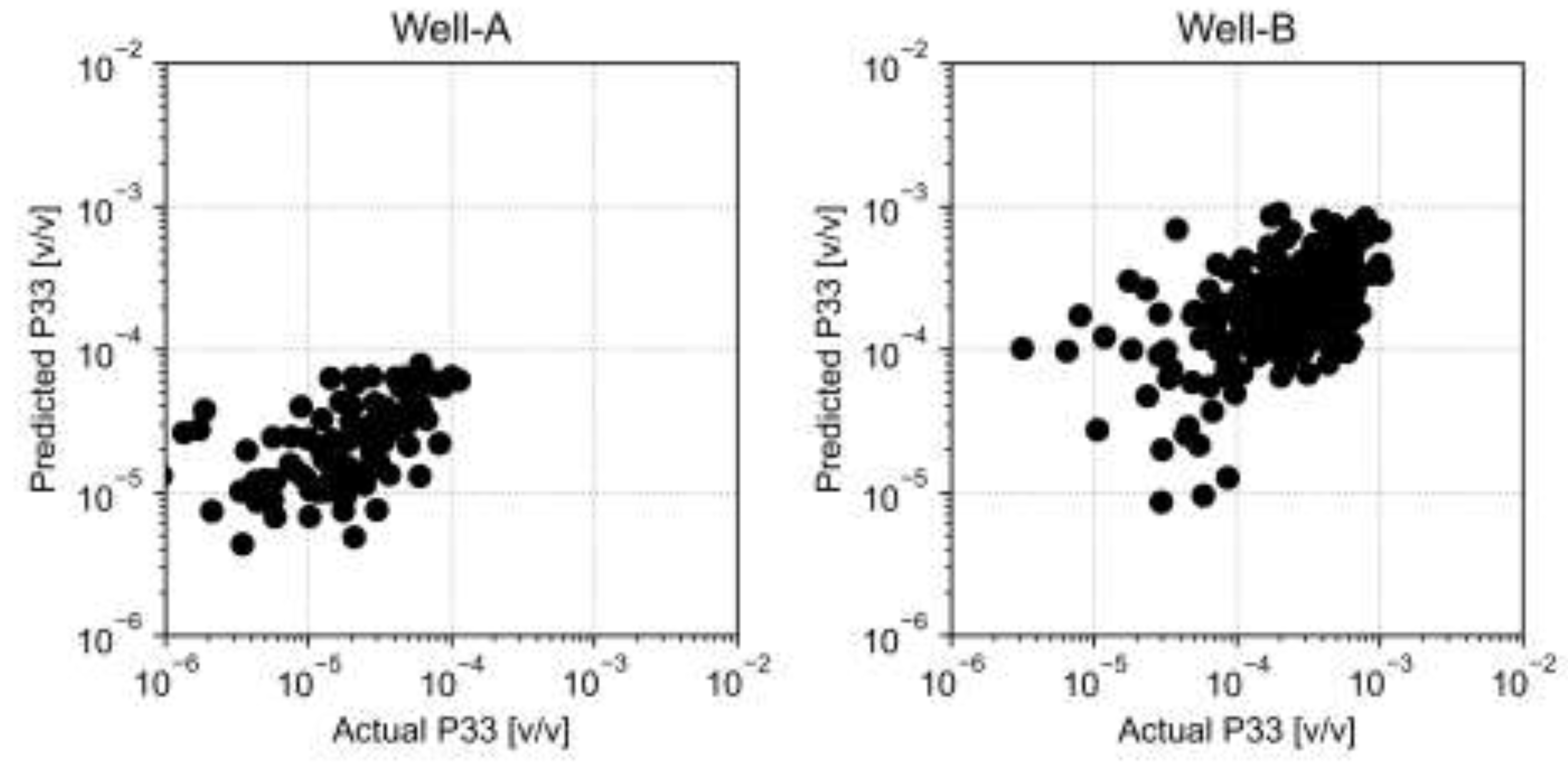

Table 1.
Statistical characteristics for the used data.
| DEPT | Cal | DTCO | DTSM | GR | P33 | PEFZ | Por | RHOZ | |
|---|---|---|---|---|---|---|---|---|---|
| (m) | (in) | (us/ft) | (us/ft) | (GAPI) | (v/v) | (b/e) | (v/v) | (g/cc) | |
| count | 5008 | 5008 | 5008 | 5008 | 5008 | 5008 | 5008 | 5008 | 5008 |
| mean | 2098.965 | 7.150779 | 64.1306 | 104.8334 | 118.4989 | 7.74E-05 | 2.788434 | 0.040624 | 2.605229 |
| std | 165.4286 | 1.339378 | 5.422916 | 13.9901 | 70.87042 | 0.00016 | 0.815019 | 0.035257 | 0.080526 |
| min | 1793.596 | 4.243306 | 46.75045 | 79.24234 | 19.42065 | 0 | 1.781257 | -0.01271 | 1.6979 |
| max | 2419.655 | 10.36588 | 88.15414 | 162.6788 | 734.3147 | 0.001278 | 10 | 0.37467 | 2.842013 |
Table 2.
Results of Root Mean Square Error (RMSE) for each well.
| RMSE | Pure ANN | Hybrid Model |
| Well-A | 0.092 | 0.083 |
| Well-B | 0.145 | 0.114 |
Disclaimer/Publisher’s Note: The statements, opinions and data contained in all publications are solely those of the individual author(s) and contributor(s) and not of MDPI and/or the editor(s). MDPI and/or the editor(s) disclaim responsibility for any injury to people or property resulting from any ideas, methods, instructions or products referred to in the content. |
© 2023 by the authors. Licensee MDPI, Basel, Switzerland. This article is an open access article distributed under the terms and conditions of the Creative Commons Attribution (CC BY) license (http://creativecommons.org/licenses/by/4.0/).
Copyright: This open access article is published under a Creative Commons CC BY 4.0 license, which permit the free download, distribution, and reuse, provided that the author and preprint are cited in any reuse.


