
Submitted:
24 June 2024
Posted:
25 June 2024
You are already at the latest version
Abstract
In this study, the determination of static E50 and υ parameters of rock materials was investigated using P-S wave velocities and Shore hardness (SH), non-destructive measurement methods. We used multiple linear regression (MLR), multiple non-linear regression (MNLR) and artificial neural network (ANN) models to estimate and determine these parameters. When the models defined by MLR, MNLR, and ANN were compared to the R2 values, ANN models that estimate E50 and υ parameters of rock materials using non-destructive methods (Vp, Vs, Vp/Vs, d, and SH) could be determined with higher accuracy than MLR and MNLR models. The study’s originality is based on the fact that ores such as galena, chromite, and barite have been studied for the first time on rock mechanics, and in this respect, it offers an innovative perspective. In addition, the use of all non-destructive measurement methods, Vp, Vs, and Shore hardness tests, also increases the originality of the study.
Keywords:
Young’s modulus
; Poisson’s ratio
; destructive/non-destructive measurement methods
; regression
; ANN modeling
1. Introduction
While determining the physicomechanical parameters of rock materials, it can be done with two methods destructive and non-destructive. While destructive methods include tests such as the uniaxial compressive strength (UCS), triaxial compressive strength (TCS), and direct (TS) and indirect tensile strength (ITS), non-destructive methods include tests such as seismic wave velocities, Schmidt and Shore hardnesses. Destructive measurement methods are generally conducted in the laboratory with specific test equipment that contains core specimens. In addition, in destructive measurement methods, when rock materials are generally weak, thin-bedded, or heavily fractured, they may not be suitable for sample preparation and measurement of mechanical tests. On the other hand, non-destructive measurement methods are based on the measurement of seismic velocities or the hardness of the rock, sometimes in situ but usually in the laboratory. Non-destructive tests are easier because it does require less sample preparation, and the test equipment is simple to use. They can also be used easily on the mine site. Therefore, non-destructive measurement methods are faster, simpler, and more economical than destructive measurement methods.
Hardness is one of the physical properties of materials and although there are many types, Schmidt and Shore hardness measurements are the best-known hardness measurement methods for rock materials. While very large rock masses are required for Schmidt hardness measurement, smaller rock pieces can also be measured for Shore hardness measurements. In addition, SH is widely used to estimate the hardness of rock materials because it is an easy-to-use and inexpensive method. Similarly, the seismic velocities (Vp and Vs) of rock materials are easy and simple to measure and take values according to the cleavage, crystalline structure, fracture structure, elasticity, porosity, and gravity properties that define the physicomechanical properties of the rock materials.
Two of the most important physicomechanical parameters of rock materials are the E50 and υ. These parameters are used in many mining operations to express the resistance of rock materials to deformation under shear or compressive stress. The E50 and υ are affected by many factors such as the crystalline structure of the rock material, cleavage, crack structure, elasticity, anisotropy state, and mineralogical composition [1,2].
Most of the engineering problems related to rock materials are caused by the incorrect evaluation of the physicomechanical properties of these materials. First of all, high-quality core samples are required to determine the E50 and υ parameters. However, sometimes it is not easy to obtain smooth cores, especially from very fractured, weak, or very hard rock materials. Moreover, even if high-quality cores can be obtained to perform tests such as UCS, TS, and ITS, it is costly, laborious, and time-consuming process in terms of human errors, instrument calibration issues, and internal factors. Therefore, engineers can estimate E50 and υ parameters from other static and dynamic rock parameters by using the estimation equations published in the literature for their required projects.
Some researchers [3,4,5,6,7,8,9,10] have conducted many studies to date on estimating E50 and υ with other static tests such as UCS, ITS, Schmidt hardness, and rock mass grade (RMR89) for different rock materials. These researchers developed many simple-linear or simple-nonlinear equations for estimating E50 or υ values. However, most of these equations were not very suitable for estimating these parameters (E50 and υ), while suitable equations gave good results only for similar rock types. Sonmez et al. (2006) [11], on the other hand, estimated E50 value using the ANN model with UCS and unit weight (γ). However, obtaining UCS and γ values is far from being an alternative for estimating E50 values, as the process of sample preparation and testing is tedious and difficult, just as E50 values are obtained. In addition, another researchers [12,13,14] tried to estimate E50 and υ with the Shore hardness (SH) test with simple-linear or simple-nonlinear regressions, but relationships were revealed with low correlation. Differently, Karakus et al. (2005) [15] proposed a good model using the MLR model to estimate E50 and υ based on the findings from some rock mechanic tests. However, the use of the point load index (Is) and uniaxial compressive strength (UCS) tests in the model could not be an alternative method because the preparation process of core samples for these tests was long and tiring.
In addition, some researchers [1,12,16,17,18,19,20,21,22,23,24,25,26] have also investigated the relationships between non-destructive measurement tests and static physicomechanical parameters of the same type of rock materials at a mining site or for a certain group of rock materials such as sedimentary, metamorphic origins, etc. When the results of these researchers were examined, it was shown that there were significant relationships between seismic velocities, especially Vp velocity, of rock samples taken from a particular group or region. Differently, Armaghani et al. (2016) [2] further investigated the estimation of E50 from Vp, porosity (n), Schmidt hardness (Rn) and point load strength (Is(50)) values for granite samples using MLR and ANN models. They not only found MLR and ANN models with very low coefficients of determination (R2=0.643 and 0.596, respectively) but also used laborious and difficult methods to determine the properties of materials such as porosity and point load strength in the models.
As can be seen from previous studies, although it is known that many test methods are widely used in estimation of physicomechanical parameters of rock materials, there are few works on the use of non-destructive measurement methods for the estimation of E50 and υ values of rock materials. Moreover, the determinant coefficients (R2) of the estimated models were low and the error values (RMSE and MAE, etc.) were high. Therefore, it is inevitable that the development of models that can estimate these parameters with easier, less laborious, less time-consuming, cheaper methods, and high accuracy will continue to be an important research topic for many researchers.
Artificial neural networks (ANNs) have attracted great attention in recent years in the estimation of various physicomechanical parameters such as UCS, ITS, shear strength parameters, and various moduli of rock materials. The reason why ANN has become especially popular lately is that the physicomechanical parameters of rock materials allow more flexible operations between variables with more input variables, due to the low coefficients of determination obtained from regression analyses such as MLR and MNLR. Therefore, ANN has great capability in modelling the physicomechanical behaviour of rock materials [27], and has been shown by many researchers to provide more accurate estimates of the physicomechanical parameters of rock materials than other statistical models. Therefore, ANN has great capability in modelling the physicomechanical behaviour of rock materials. Some researchers [2,28,29,30,31,32,33,34] have shown that ANNs provide much more realistic estimations than other statistical models for estimating the physicomechanical parameters of rock materials.
In this study, models have been tried to be developed to estimate E50 and υ of rock materials with ultrasonic wave velocities (Vp and Vs), dynamic density (ρd) and Shore hardness (SH) tests which are the non-destructive measurement methods. These non-destructive measurement methods do not require special specimen preparation requirements such as coring and large specimen sizes. Also, they are also much easier to use compared to the stress-strain tests used to obtain E50 and υ values. These non-destructive tests can be used to estimate, rather than the measure E50 and υ values. The main advantages of non-destructive measurement methods are known for their ease of use and flexibility.
This study aims to estimate E50 and υ obtained by stress-strain curves under compression from non-destructive measurement methods (Vp, Vs, Vp/Vs, ρd, and SH) using the MLR, MNLR, and ANN models. In this study, a series of analyses were carried out on a total of 17 different rock materials of geological origin, including sedimentary (8), metamorphic (2), igneous-volcanic (4), and mafic-ultramafic igneous ores (3). In general, and so far almost all of the rock mechanics tests have been carried out on rock materials of sedimentary (limestone, gypsum, etc.), metamorphic (marble, feldspar, etc.), and volcanic (andesite, trass, etc.) origin. This study will be the first study on a very different sample group, including mafic and ultramafic igneous ores such as sulfide ore, galena, and chromite. In this respect, it would make an important contribution to the literature.
2. Materials and Methods
2.1. Materials
A total of 17 different rock types were collected, 8 are sedimentary, 2 are metamorphic, 4 of them are igneous-volcanic, and 3 are mafic and ultramafic igneous ores, from various regions of Turkey. The mineralogical properties of the rock materials used in the tests were shown in Table 1.
As shown in Figure 1a–d, core samples of 54 mm diameter were prepared from rock blocks collected in the laboratory. In non-destructive experimental studies, Vp and Vs were first measured on these core specimens with a sonic wave viewer, and then Shore hardness (SH) were measured on the same core specimens with a Shore Scleroscope C-2 (as seen in Figure 1(g)).
In destructive experimental studies, according to the test procedures recommended by ASTM D7012-14e1 (2017) [35], stress-strain measurements were performed on core specimens under compression, as shown in Figure 1(e-f). The static E50 and υ values were calculated from the stress-strain curves which were simultaneously recorded using a computer. After the destructive and non-destructive tests, statistical modeling studies were started. While Vp, Vs wave velocities (m/sec), Vp/Vs ratios, dynamic densities (ρd, t/m3), and Shore hardness (SH) values were also used as input data in the modeling, E50 and υ values were then considered as output data.
2.2. Sonic Wave Velocity (Vp and Vs) Tests
In this study, sonic wave velocity measurements (Vp and Vs) were applied according to the ASTM D2845-08 (2008)[36] standard. For the measurement of Vs and Vp, specimens should be cylindrical (core) or cubical or cut straight so that both sides of the specimens are parallel (Figure 2 (a)). The easiest among them is to cut the samples neatly from both sides. For this, samples can be cut on a rock cutting machine. In our study, sonic velocity tests were performed on a total of 10-15 core specimens taken from three directions (3-5 cores from each direction) to determine the static E50 and υ values, taking into account the anisotropy condition for each rock block sample.
The OYO sonic viewer (Model 5217-A), which includes a battery, a receiver, a transmitter, an ultrasonic pulse generator, and a signal data acquisition and display system (as shown in Figure 2 (b)), was used to measure the ultrasonic wave velocities (Vp and Vs) of rock materials. Before the ultrasonic wave velocity, the ends of the core specimens were polished and a thin layer of grease was applied. The ultrasonic wave (Vp and Vs ) velocities are calculated from the travel time of the measured wave and the distance between the transmitter and receiver, i.e. the measured sample length.
The density value of a rock material has an important factor in engineering studies. We can determine the density of a rock material directly (destructive method) by measuring it, as well as indirectly (non-destructive method) by calculating it. It requires examining samples in the laboratory by gradual grinding to less than 100 microns in order for the density to be directly determined. This is a time-consuming and tedious process. For this reason, many researchers have been working to determine the density value indirectly from seismic wave velocities (Vp and Vs) since the 1970s. Telford et al. (1976) [37] investigated the relationship between the density of rock materials and seismic wave velocities, and they stated that the dynamic density of rock materials can be found from the P-wave velocity (Vp), as can be seen in Eq. (1) given below.
ρd = 0.2Vp+1.6,
2.3. Shore Hardness Tests
The Shore hardness instrument is a non-destructive measuring instrument on relatively small specimens and measures the relative values of Shore hardness (SH) with a diamond-tipped hammer that falls freely from top to bottom onto a smooth specimen [38]. ISRM (1981) [39] has proposed a method for the C-2 model Shore hardness instrument for rock materials.
Specimens can also be created for SH measurements similar to ultrasonic wave velocity measurements cylindrical (core) or cubic from rock blocks or smoothly cutting from both sides of rock specimen. The method of smooth cutting from both sides of the rock specimens has become an easy method to determine SH, especially if specimens are small in size or cannot be cored. In this study, Shore hardness measurements were also carried out after ultrasonic wave velocity tests were performed on the core samples. Shore hardness measurements were accepted as the SH of the rock material by taking the arithmetic average of about 200 readings from about 10 cores, with at least 20 readings from each core specimen.
2.4. The Stress-Strain Tests to Determine E50 and υ Values
In this study, cylindrical specimens (cores of 108 mm length and 54 mm diameter) were used for measuring E50 and υ values of rock materials. To meet the statistical requirements, at least 15 core specimens were used for each rock sample. E50 and υ tests were carried out according to ASTM’s recommended methods [35]. Stress-strain measurement is carried out by using an electronic servo-controlled UCS testing machine (Figure 1 (f)). The case where electrical resistance lateral and axial strain gauges, bonded to core specimens, was shown in Figure 1(e). E50 is defined as the ratio of axial stress to axial strain under compression, and it is obtained by plotting the axial stress versus axial strain curve and measuring the slope of the curve. On the other hand, υ is the absolute value of the ratio of lateral strain to axial strain under compression, and it is dimensionless and ranges between 0.01 and 0.5.
3. Results and Discussion
In this study, output (Y) the static Poisson’s ratio (υ)or Young’s modulus (E50) of the rock materials were characterized as the function of the Vp (X1), Vs (X2), Vp/Vs (X3), ρd (X4), and SH (X5). The important statistical properties such as minimum, maximum, mean, and standard deviation with E50 and υ of all variables were given in Table 2.
3.1. MLR and MNLR Analysis
The relationships between independent variables and dependent variables can be investigated by using the MLR or MNLR analyses. In estimating the value, MLR models are expressed linearly and MNLR models are expressed as a non-linear function. The choice between MLR and MNLR models is determined by the high determination coefficient of the relationships to be obtained [2,40].
The relationships between independent variables and dependent variables can be investigated by using the MLR or MNLR analyses. In estimating the value, MLR models are expressed linearly and MNLR models are expressed as a non-linear function. The choice between MLR and MNLR models is determined by the high determination coefficient of the relationships to be obtained [2,40].
Y= β0+β1X1+β2X2+β3X3+β4X4+ . . . +βnXn ,
MNLR analysis estimates the model by forming a random non-linear relationship between one or more independent variables and a dependent variable. The typical form of the nonlinear relationship is considered to be as in Eq. (3).
Y= β0(X1β1)(X2β2)(X3β3)(X4β4) . . . (Xnβn) ,
Where, while Y is the dependent variable, X1, X2, X3, X4,…, Xn are independent variables. While β0 is the constant value, β1, β2, β3, β4,…, βn are the regression coefficients of linear or non-linear independent variables [40,41,42].
When multiple regression analysis is applied, it is absolutely necessary to check whether there are autocorrelation and multicollinearity problems between independent variables. ANOVA and coefficient tables help explain whether the regression equation is statistically significant. In order to evaluate how well the resulting model fits the experimental data, the decision is made by looking at R2, F, and p values. While the coefficient of determination (R2) value reveals the significance of the relationship established between one dependent and one or more independent variables, the F value is used to determine the significance of R2. R2 value takes a maximum value of 1, and the closer R2 value is to 1, the more accurately the model represents. On the other hand, F and p values indicate whether the model is statistically significant or not. The higher the F values obtained from the F-test, the more significant the model is. Also, the significance levels (p values) of the T-test are taken into account to evaluate the performance of the regression methods. The significance values (p) should be less than 0.05 (the confidence level of 95%). All possible combinations of independent variables are considered and checked for multicollinearity in any of them. Those independent variables with multicollinearity problems are removed from the model [43].
Additionally, variance increase factor (VIF), Tolerance (T), and Durbin-Watson (D-W) factors are also taken into account to determine whether there is autocorrelation between the independent and dependent variables. If the VIF values are less than 10.0, the average VIF value is less than 3.0, and the tolerance (T) values are greater than 0.10, it shows that the variables are independent of each other and the regression model is strong. When the T value approaches zero, this means that each independent variable is autocorrelated with other independent variables. Similarly, the closer the D-W value (it takes values between 0 and 4) is to 2, it means that there is no autocorrelation between the independent variables [43]. All statistical parameters (R2, F, p, VIF, T, and D-W) were used in this study to check whether there are autocorrelations between the independent variables, and such problematic independent variables were excluded from the model.
MLR and MNLR analyses are carried out using a computer software package program since they involve quite complex calculations. In this study, the IBM SPSS 22 statistical software package was used to generate MLRs between five independent variables (Vp, Vs, Vp/Vs, ρd, and SH) and a dependent variable as output (E50 or υ). The stepwise method in the SPSS program commonly used in this type of modeling is a technique for constructing a model by adding or subtracting estimative parameters through a series of F-tests or T-tests. The E50 and υ values of the rock materials were introduced as dependent variables (outputs) and X1 (Vp, m/sec), X2 (Vs, m/sec), X3 (Vp/Vs), X4 (ρd), and X5 (SH), as independent variables (inputs). However, the p-value and Tolerance of Vp/Vs and SH were calculated as near 0 before the MLR was processed, which means that the Vp/Vs and SH variance has the highest multicollinearity probability when all variables are taken into account, therefore, Vp/Vs and SH were eliminated from the model. As a result, the most reliable regression equations for the determination of E50 and υ values by MLR analysis can be obtained with the Eq. (4) and Eq. (5) given below.
E50 = −22.613−0.001*(Vp)+14.576(ρd), R2=0.582 ,
υ = 0.575−4.066*10-5*(Vs)−0.055*(ρd), R2=0.486 ,
When the independent variables are evaluated in terms of autocorrelation and multicollinearity, as seen in Eq. (4) and Eq. (5), three potential independent variables (Vs, Vp/Vs, and SH) were neglected for E50, while two independent variables (Vs and ρd) could be evaluated for υ.
Some non-linear regression equations can be converted to a linear equation with an appropriate transformation of the model equation. If the logarithm to base e of Eq. (3) was taken, it becomes a linear relationship as in Eq.(6) [42].
and so, an Ln(Y) regression over Ln(X1), Ln(X2), Ln(X3), Ln(X4), and Ln(X5) are used to estimate parameters β0, β1, β2, β3, β4, β5 and βn [42].
Ln(Y)= Ln(β0)+β1Ln(X1)+β2Ln(X2)+β3Ln(X3)+β4Ln(X4)+β5Ln(X5) . . . βnLn(Xn),
The β0, β1, β2, β3, β4, β5, and βn coefficients were determined using the stepwise method in SPSS 22 package program. The stepwise method commonly used in this type of modeling is a technique for constructing a model by adding or subtracting estimative parameters through a series of F-tests or T-tests. The model expressions were coded into the solver based on the fitting result of the linear regression solver and a series of iterations were run. Iteration runs were now stopped when the relative reduction between sums of squares was minimized.
In this study, regression relationships between five independent variables and one dependent variable (E50 or υ) were revealed. In both regression relationship equations, the dependent variables X1, X2, X3, X4, and X5 are Vp, Vs, Vp/Vs, ρd, and SH, respectively. βi coefficients were estimated from the experimental results using the SPSS program that applies the least-square method. R2, VIF, T, and p-values were taken into account to evaluate the estimative performance of the regression equations. Then, the best independent variables that did not show autocorrelation and multicollinearity were selected. As a result, the following equations were obtained by MNLR analysis using the best independent variables.
Ln(E50) = 11.519*(Vp)-0.716*(ρd)-5.868 , R2=0.591 ,
Ln(υ) = 0.6555*(Vp)0.768*(Vs)-0.843*(ρd)-0.713 , R2=0.630 ,
When the independent variables are evaluated in terms of autocorrelation and multicollinearity, as seen in Eq. (7) and Eq. (8), three potential independent variables (Vs, Vp/Vs, and SH) were neglected for E50, while three independent variables (Vp, Vs, and ρd) could be evaluated for υ.
As a result of regression analyses, E50 and υ values were estimated using Eq. (4) and Eq. (5) by MLR analysis and Eq. (7) and Eq. (8) by MNLR analysis, and these equations were determined with low coefficients of determination (R2). In addition, since it is not expressed with two independent variables (Vp/Vs and SH), it is not suitable to be considered a reliable model for E50 and υ estimation. Therefore, as a solution to such problems, soft computation methods such as ANN can be used.
3.2. ANN Analysis
Using an ANN, a neural network model can be created that can estimate the desired output from one or more inputs. ANN model has become a widely used modeling tool in many applications owing to its higher accuracy than an MNLR in modeling multivariate problems. The fact that ANN is preferred over classical modeling methods comes from its non-linearity, learning ability, ability to process fuzzy information, and generalization ability. Although, various ANN types are used in the literature, feed-forward ANN is the most preferred. The feed-forward ANN is a multilayer perceptron neural network (MLP-ANN). In order for an ANN to create an accurate model, it must first be trained. Among the different learning algorithms for training MLP-ANN, the most widely used is the backpropagation (BP) algorithm. The backpropagation ANN (BP-MLP-ANN) has been successfully used as an estimating tool in many fields so far [11,34,44].
The simplest form of MLP-ANN consists of an input layer, a hidden layer, and an output layer. Each layer is made up of neurons (nodes), and neurons from the input layer are connected by weighted connections to neurons in the hidden layer which are connected to neurons in the output layer. Several interconnected neurons can be used to construct an ANN. During the learning phase, the interconnections are optimized in order to minimize a predefined non-linear activation function. This process is repeated continuously until the output is produced [44,45]. The general system structure of a backpropagation MLP-ANN is shown in Figure 3 (a) and the hyperbolic tangent activation function is shown in Figure 3 (b).
In this study, a multilayer perceptron network with hidden layers and an MLP-ANN with backpropagation architecture were developed using the neural network function in the SPSS 22.0 program. An ANN model usually has three layers: input layers, hidden layers, and output layers. The input layer was created from five source points such as Vp, Vs, Vp/Vs, ρd, and SH. The hidden layer was a non-linear processing unit and could have more than one. The output layer was evaluated by the network and produced E50 or υ, which are the desired result points from the model. The most applied transfer functions in the literature are sigmoid and hyperbolic tangent activation functions. In this study, the hyperbolic tangent activation function was preferred because it provided the most effective approach. On the other hand, no function was used in the output layer. Additionally, 75% of the data was used for training and 25% was used in the testing stage. Five combinations of the variables (Vp, Vs, Vp/Vs, ρd, and SH) were investigated with SPSS to determine the optimal network architecture. The best input combinations of the ANN models were given in Table 3. These models were selected based on the highest determination coefficient (R2), the lowest root mean square error (RMSE), and the lowest mean absolute error (MAE) to estimate Es and υ values of rock materials.
In the study, the hyperbolic tangent function shown in Eq. (9) with the output range of [−1, 1] was used. Further, the R2, MAE, and RMSE equations shown in Eq. (10), Eq. (11), and Eq. (12) were used to verify the validity of selected models.
 where n, yi, ў, and ŷi are the number of experiment, the experimental values, the mean of the experimental values, and the estimated values, respectively.
R2, RMSE, and MAE values calculated to determine the validity of ANN models are presented in Table 3. When Table 3 is examined, R2 values higher than 0.80 mean that there are relationships with acceptable accuracy for these four models. However, when the R2, RMSE, and MAE values in Table 3 were examined, it was determined that ANN-2 gave more accurate estimates than other models. The R2 values of 0.965 and 0.971 obtained by the ANN-2 model for E50 and υ, respectively, indicate that the models have a very high relationship. The estimation error values for the E50 and υ were 0.883 and 0.006 for the RMSE and 0.699 and 0.004 for the MAE, respectively. The ANN-3 was ranked as the second-best. The results of the ANN-1 and ANN-4 models were also acceptable to estimate E50 and υ. When normalized importance values are examined, the Shore hardness (SH) was found to have a great effect of 100% on both E50 value and υ value.
Figure 4 shows the best model architecture (ANN-2), which consist of one input layer of 4 variables, one hidden layer of 10 neurons, and one output layer of one variable (4-10-1 structure) by using the activation functions. Additionally, in Figure 5, the predicted values of Es and υ are plotted against the experimental values to analyze the accuracy of the ANN-2 model.
3.3. Comparision of Models
The E50 and υ parameters of rock materials were compared in terms of the estimated values using MLR, MNLR, and ANN models. As a result, it was revealed that MLR and MNLR models could not estimate both E50 and υ parameters very well. Additionallly, due to the complexity of the fracture process of rock materials, it is an expected result that the coefficients of determinate (R2) of the MLR and MNLR models for E50 and υ are low. On the other hand, ANN models with the highest R2 values in estimating E50 and υ parameters were found to be much more suitable than MLR and MNLR models.
A comparison of the estimated values of the ANN-2 for each of the 17 experimental data of E50 and υ of rock materials is shown in Figure 6. Apparently, it shows that the ANN-2 model was able to estimate both E50 and υ values very well within the acceptance limit. On the other hand, the estimated values of other ANN models were significantly different in accuracy from all experimental E50 and υ values. In addition, the ANN-2 model, which has the least RMSE and MAE and the highest R2 values (in Table 3), shows that it will be much more suitable than other ANN models.
Although it is generally accepted that a lot of data is needed to train the neural network, it is important that ore samples such as galena, chromite, and sulfur ore, which have not been used in any study before, are used for the first time in this study.
4. Conclusions
This research work aims to develop estimation models with the highest accuracy for the determination of E50 and υ parameters of rock materials with non-destructive measurement methods (Vp, Vs, Vp/Vs, ρd, and SH). For this purpose, 17 different rock materials were considered and multiple measurements were made to estimate E50 and υ with the best accuracy.
Model approaches were based on input data (Vp, Vs, Vp/Vs, ρd, and SH). Their use has not performed satisfactory results with data in multiple regression analyses (MLR and MNLR) expressed as correlation coefficients (R2=0.486-0.630). However, ANN models developed with the same experimental data produced results with higher determination coefficients (R2=0.891-0.971). These results show that ANN models can be preferred for estimation and evaluation of E50 and υ compared to regression analysis models. From these results, it was determined that all four ANN models were able to predict both E50 and υ with higher accuracy and very small errors. Among the ANN architecture tested, ANN-2, 4 input variables (Vp, Vs, Vp/Vs, and SH), 10 neurons, and one output variable (E50 or υ), was the best architecture (4-10-1 structure). In addition, the results of sensitivity analysis of both E50 and υ values to input variables showed that Shore hardness (SH) was the most sensitive variable.
In this study, it is important for the literature that a very different sample set including magmatic ores such as chromite, galena, and sulfide ores was used in modeling. It is clear that such estimation models will be much more beneficial to the engineers in the sector if different geological types and more numerous specimen sets are evaluated for similar research in the coming years.
Author Contributions
Conceptualization, V.D. and O.T.D.; methodology, V.D.; software, V.D. and O.T.D.; data curation, V.D. and O.T.D.; writing—original draft preparation, O.T.D.; writing—review and editing, V.D.; visualization, O.T.D.; supervision, V.D. All authors have read and agreed to the published version of the manuscript.
Funding
This research received no external funding.
Conflicts of Interest
The authors declare no conflicts of interest.
References
- King, M.S. Static and dynamic properties of rocks from the Canadian Shield. Int. J. Rock Mech. Min. Sci.Geomech. Abst. 1983, 20, 237–245. [Google Scholar] [CrossRef]
- Armaghani, D.J. , Mohamad, E.T., Momeni, E., Monjezi, M., Narayanasamy, M.S. Prediction of the strength and elasticity modulus of granite through an expert artificial neural network. Arab. J. Geosci. 2016. [Google Scholar] [CrossRef]
- Sachpazis, C.I. , Correlating Schmidt hardness with compressive strength and Young’s modulus of carbonate rocks. Bull. Int. Assoc. Eng. Geol. 1990, 42, 75–83. [Google Scholar] [CrossRef]
- Yilmaz, I. , Sendir, H. Correlation of Schmidt hardness with unconfined compressive strength and Young’s modulus in gypsum from Sivas (Turkey). Eng. Geol. 2002, 66, 211–219. [Google Scholar] [CrossRef]
- Hoek, E. , Diederichs, M.S. Empirical estimation of rock mass modulus. Int. J. Rock Mech. Min. Sci. 2006, 43, 203–215. [Google Scholar] [CrossRef]
- Isik, N.S. , Ulusay, R., Doyuran, V. Deformation modulus of heavily jointed–sheared and blocky greywackes by pressure meter tests: Numerical, experimental and empirical assessments. Eng. Geol. 2008, 101, 269–282. [Google Scholar] [CrossRef]
- Palchik, V. On the ratios between elastic modulus and uniaxial compressive strength of heterogeneous carbonate rocks. Rock Mech. Rock Eng. 2011, 44, 121–128. [Google Scholar] [CrossRef]
- Alemdag, S. , Gurocak, Z., Gokceoglu, C. A simple regression based approach to estimate deformation modulus of rock masses. J. Afr. Earth Sci. 2015, 110, 75–80. [Google Scholar] [CrossRef]
- Feng, X. , Jimenez, R. Estimation of deformation modulus of rock masses based on Bayesian model selection and Bayesian updating approach. Eng. Geol. 2015, 199, 19–27. [Google Scholar] [CrossRef]
- Ghafoori, M. , Rastegarnia, A., Lashkaripour, G.R. Estimation of static parameters based on dynamical and physical properties in limestone rocks. J. Afr. Earth Sci. 2018, 137, 22–31. [Google Scholar] [CrossRef]
- Sonmez, H. , Gokceoglu, C., Nefeslioglu, H.A., Kayabasi, A. Estimation of rock modulus: for intact rocks with an artificial neural network and for rock masses with a new empirical equation. Int. J. Rock Mech. Min. Sci. 2006, 43, 224–235. [Google Scholar] [CrossRef]
- Yasar, E. , Erdogan, Y. Estimation of rock physicomechanical properties using hardness methods. Eng. Geol. 2004, 71, 281–288. [Google Scholar] [CrossRef]
- Shalabi, F.I. , Cording, E.J., Al-Hattamleh, O.H. Estimation of rock engineering properties using hardness tests. Eng. Geol. 2007, 90, 138–147. [Google Scholar] [CrossRef]
- Teymen, A. Statistical models for estimating the uniaxial compressive strength and elastic modulus of rocks from different hardness test methods. Heliyon 2021, 7. [Google Scholar] [CrossRef]
- Karakus, M. , Kumral, M., Kilic, O. Predicting elastic properties of intact rocks from index tests using multiple regression modeling. Int. J. Rock Mech. Min. Sci. 2005, 42, 323–330. [Google Scholar] [CrossRef]
- Van Heerden, W.L. General relations between static and dynamic moduli of rocks. Int. J. Rock Mech. Min. Sci. Geomech. Abstr. 1987, 24, 381–385. [Google Scholar] [CrossRef]
- Kahraman, S. , Yeken, T. Determination of physical properties of carbonate rocks from P-wave velocity. Bull. Eng. Geol. Environ. 2008, 67, 277–281. [Google Scholar] [CrossRef]
- Sharma, P.K. , Singh, T.N. A correlation between P-wave velocity, impact strength index, slake durability index and uniaxial compressive strength. Bull. Eng. Geol. Environ. 2008, 67, 17–22. [Google Scholar] [CrossRef]
- Yagiz, S. P-wave velocity test for assessment of geotechnical properties of some rock materials. Bull. Mater. Sci. 2011, 4, 947–953. [Google Scholar] [CrossRef]
- Khandelwal, M. Correlating P-wave velocity with the physic-mechanical properties of different rocks. Pure Appl. Geophys. 2013, 170, 507–514. [Google Scholar] [CrossRef]
- Concu, G.De. , Nicolo, B., Valdes, M. Prediction of building limestone physical and mechanical properties by means of ultrasonic P-wave velocity. Sci. World J. 2014. [Google Scholar] [CrossRef] [PubMed]
- Pappalardo, G. Correlation between P-wave velocity and physical-mechanical properties of intensely jointed dolostones, Peloritani mounts, NE Sicily. Rock Mech. Rock Eng. 2015, 48, 1711–1721. [Google Scholar] [CrossRef]
- Raj, K. , Pedram, R. Correlations between direct and indirect strength test methods. Int. J. Min. Sci. Technol. 2015, 25, 355–360. [Google Scholar]
- Chen, X. , Xu, Z. The ultrasonic P-wave velocity-stress relationship of rocks and its application. Bull. Eng. Geol. Environ. 2016, 76, 661–669. [Google Scholar] [CrossRef]
- Korkanc, M. , Solak, B. Estimation of engineering properties of selected tuffs by using grain/matrix ratio. J. Afr. Earth Sci. 2016, 120, 160–172. [Google Scholar] [CrossRef]
- Stan-Kłeczek, I. The study of the elastic properties of carbonate rocks on a base of laboratory and field measurement. Acta Montan. Slovaca 2016, 21, 76–83. [Google Scholar]
- Huang, Y. , Wänstedt, S. The introduction of neural network system and its applications in rock engineering. Eng. Geol. 1998, 49, 253–260. [Google Scholar] [CrossRef]
- Meulenkamp, F. , Alvarez-Grima, M. Application of neural networks for the prediction of the unconfined compressive strength (UCS) from Equotip hardness. Int. J. Rock Mech. Min. Sci. 1999, 36, 29–39. [Google Scholar] [CrossRef]
- Baykasoglu, A. , Gullu, H., Canakcı, H., Ozbakır, L. Prediction of compressive and tensile strength of limestone via genetic programming. Expert Sys. Appl. 2008, 35, 111–123. [Google Scholar] [CrossRef]
- Zorlu, K. , Gokceoglu, C., Ocakoglu, F., Nefeslioglu, H.A., Acikalin, S. Prediction of uniaxial compressive strength of sandstones using petrography-based models. Eng. Geol. 2008, 96, 141–158. [Google Scholar] [CrossRef]
- Dehghan, S. , Sattari, G.H., Chehreh, C.S., Aliabadi, M.A. Prediction of unconfined compressive strength and modulus of elasticity for travertine samples using regression and artificial neural. New Min. Sci. Technol. (China). 2010, 20, 41–46. [Google Scholar] [CrossRef]
- Jang, H. , Topal, E. Optimizing over break prediction based on geological parameters comparing multiple regression analysis and artificial neural network. Tunn. Undergr. Space Technol. 2013, 38, 161–169. [Google Scholar] [CrossRef]
- Momeni, E. , Armaghani, D.J., Hajihassani, M., Amin, M.F.M. Prediction of uniaxial compressive strength of rock samples using hybrid particle swarm optimization-based artificial neural networks. Measurement. 2015, 60, 50–63. [Google Scholar] [CrossRef]
- Mottahedi, A. , Sereshki, F., Ataei, M. Development of overbreak prediction models in drill and blast tunneling using soft computing methods. Eng. Comput. 2018, 34, 45–58. [Google Scholar] [CrossRef]
- ASTM D7012-14e1. Standard test methods for compressive strength and elastic moduli of intact rock core specimens under varying states of stress and temperatures, American Society for Testing and Materials International, West Conshohocken, Pennsylvania, USA, 2017. [CrossRef]
- ASTM D2845-08, Standard test method for laboratory determination of pulse velocities and ultrasonic elastic constants of rock (Withdrawn 2017), American Society for Testing and Materials International, West Conshohocken, Pennsylvania, USA, 2008. [CrossRef]
- Telford, W.M., Geldart, L.P., Sheriff, R.E., Keys, D.A. Applied Geophysics; Cambridge University Press: Cambridge, UK, 1976. [Google Scholar]
- Tumac, D. , Bilgin, N., Feridunoglu, C., Ergin, H. Estimation of rock cuttability from Shore hardness and compressive strength properties. Rock Mech. Rock Eng. 2007, 40, 477–490. [Google Scholar] [CrossRef]
- ISRM, Suggested methods for determining hardness and abrasiveness of rocks, Part 3. In E.T. Brown (editor), Rock characterization, testing and monitoring: ISRM suggested methods, Pergamon, U.K., 1981; pp. 101–103.
- Kutner, M.H. , Nachtsheim, C.J., Neter, J., Li, W. In Applied Linear Statistical Models, 5th ed.; McGraw-Hill Higher Education: New York, USA, 2004. [Google Scholar]
- Paulson, D.S. Handbook of regression and modeling. Chapman & Hall/CRC, Taylor&Francis Group, Florida, USA, 2007.
- Bilgili, M. , Ozgoren, M. Daily total global solar radiation modeling from several meteorological data. Meteorol. Atmos. Phy. 2011, 112, 125–138. [Google Scholar] [CrossRef]
- Hair, JF.Jr., Anderson, R.E., Tatham, R.L., Black, W.C. Multivariate Data Analysis,, 5th ed.; Prentice Hall PTR: New York, USA, 1998. [Google Scholar]
- Jain, A.K., Mao, J., Mohiddin, K.M. Artificial neural networks: a tutorial. Comp. IEEE 1996, 29, 31–44. [Google Scholar] [CrossRef]
- Schalkoff, R.J. Artificial neural network; McGraw-Hill: McGraw-Hill, New York, USA, 1997. [Google Scholar]
Figure 1.
The core specimens taken from rock blocks such as gypsum (a), marble (b), trass (c), galen (d), electrical resistance lateral and axial strain gauges glued to the feldspar core specimen (e), strain-gauge bonded rock specimen under compression (f), Shore Scleroscope C-2 using in the experiments (g).
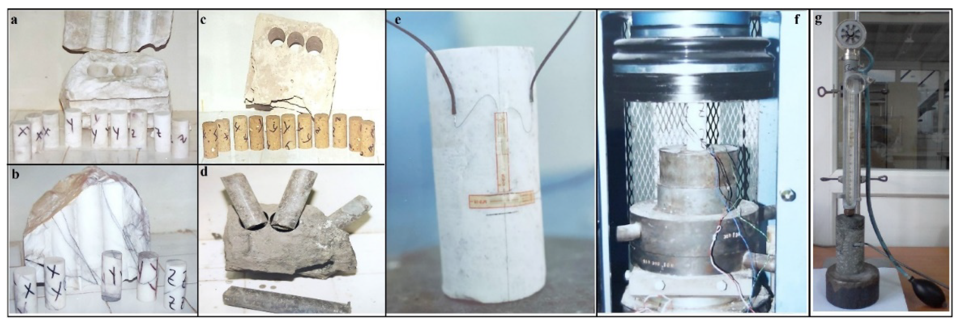
Figure 2.
Specimen types used for sonic wave velocity measurement (a), working principle of sonic viewer instrument used in experiments (b).
Figure 2.
Specimen types used for sonic wave velocity measurement (a), working principle of sonic viewer instrument used in experiments (b).
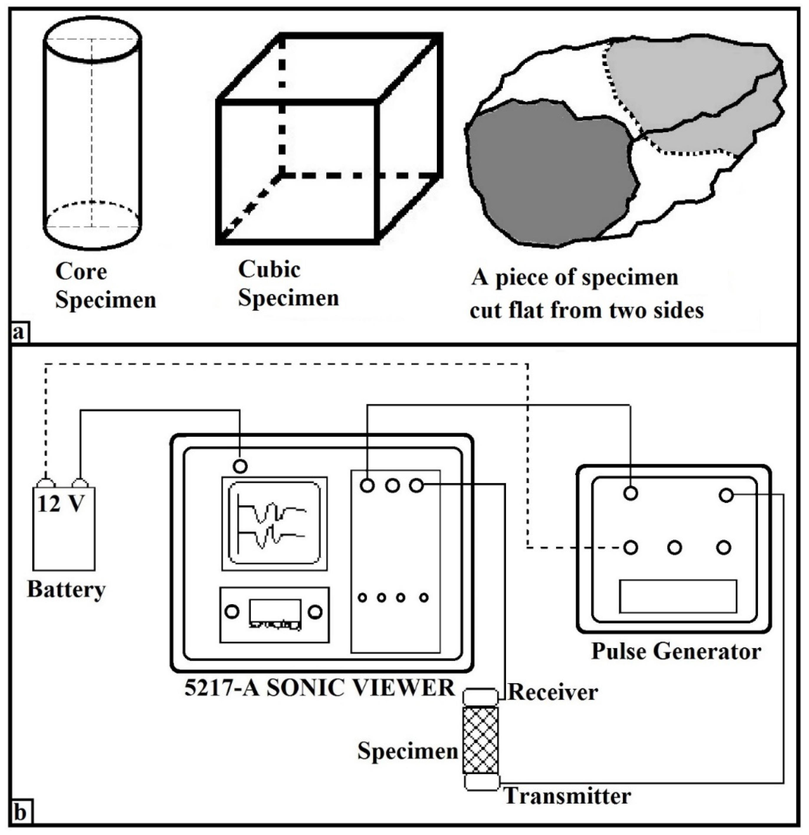
Figure 3.
Architecture of an ANN model structure (a) and hyperbolic tangent activation function (b).
Figure 3.
Architecture of an ANN model structure (a) and hyperbolic tangent activation function (b).
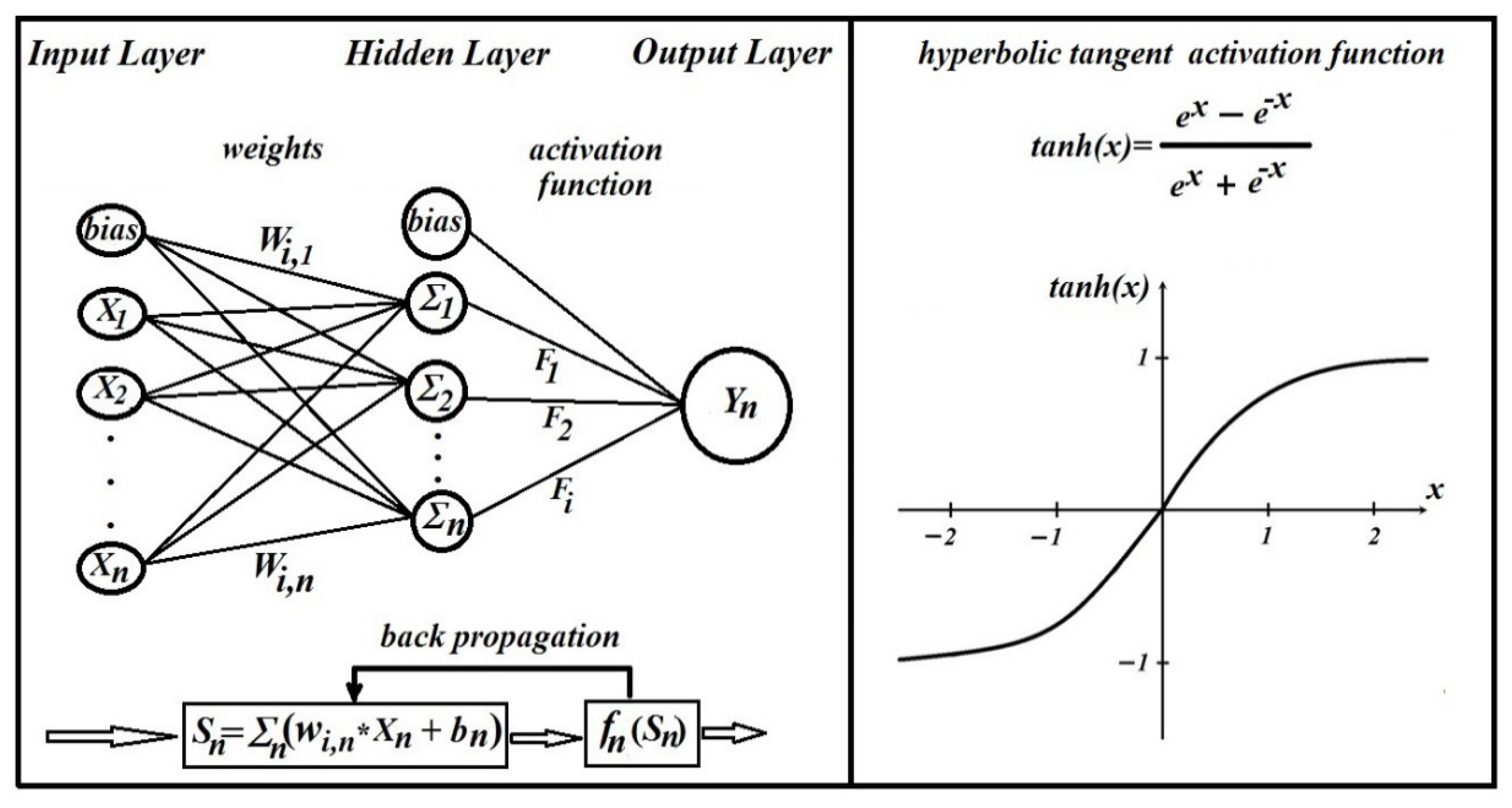
Figure 4.
Architecture of ANN-2 model used to estimate the E50 (a) and υ (b) of the rock materials.
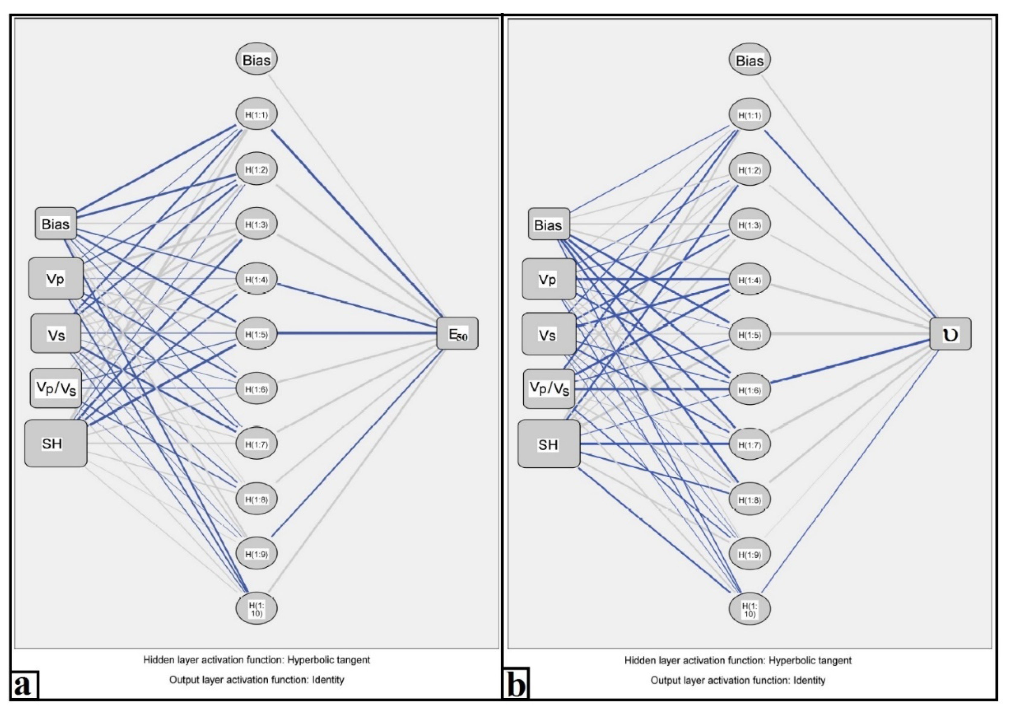
Figure 5.
Comparison of the ANN-2 estimated values and the experimental values for E50 (a) and υ (b) of the rock materials.
Figure 5.
Comparison of the ANN-2 estimated values and the experimental values for E50 (a) and υ (b) of the rock materials.
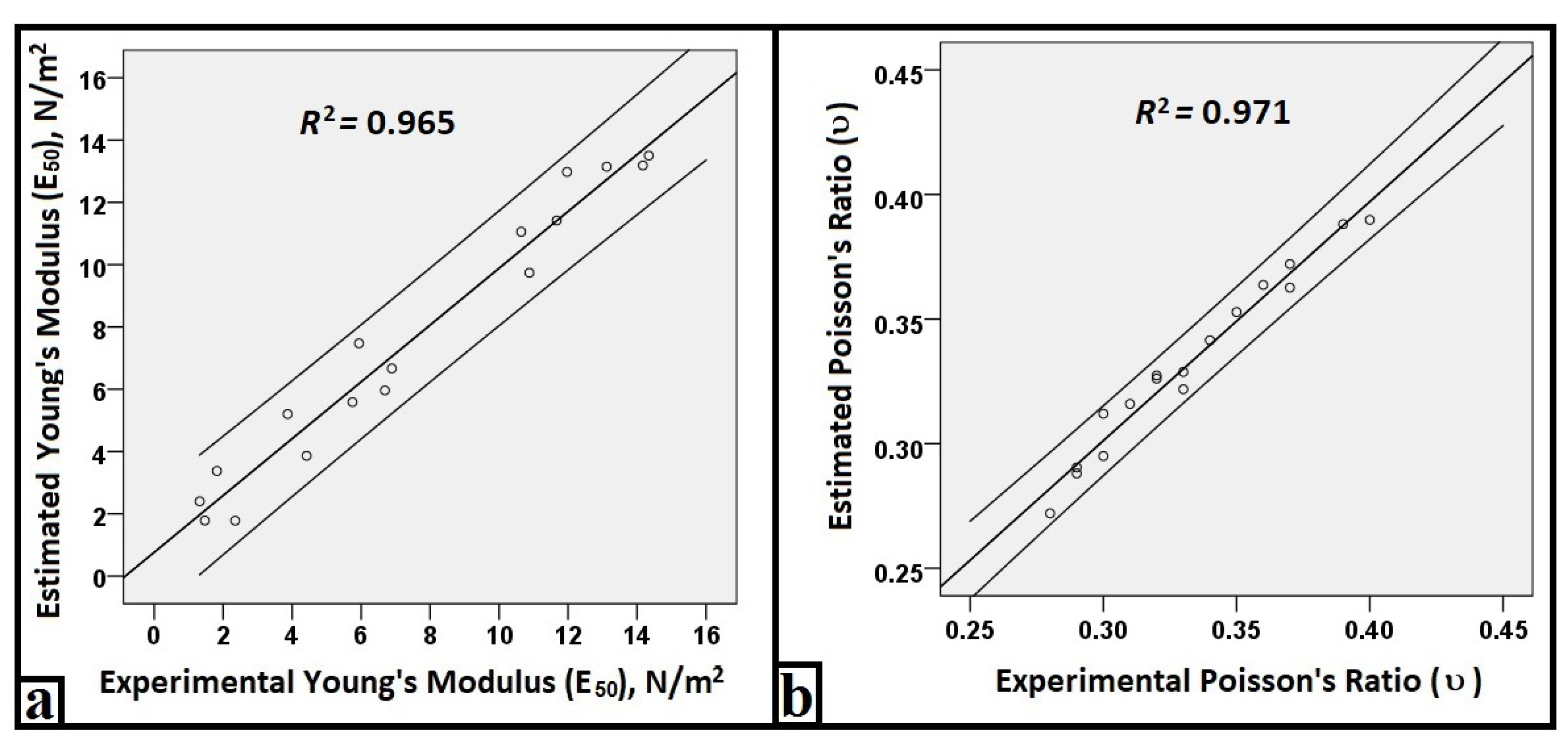
Figure 6.
Comparison plots of the estimated values by the ANN-2 model with values of experimental E50 (a) and υ (b) of the rock materials.
Figure 6.
Comparison plots of the estimated values by the ANN-2 model with values of experimental E50 (a) and υ (b) of the rock materials.
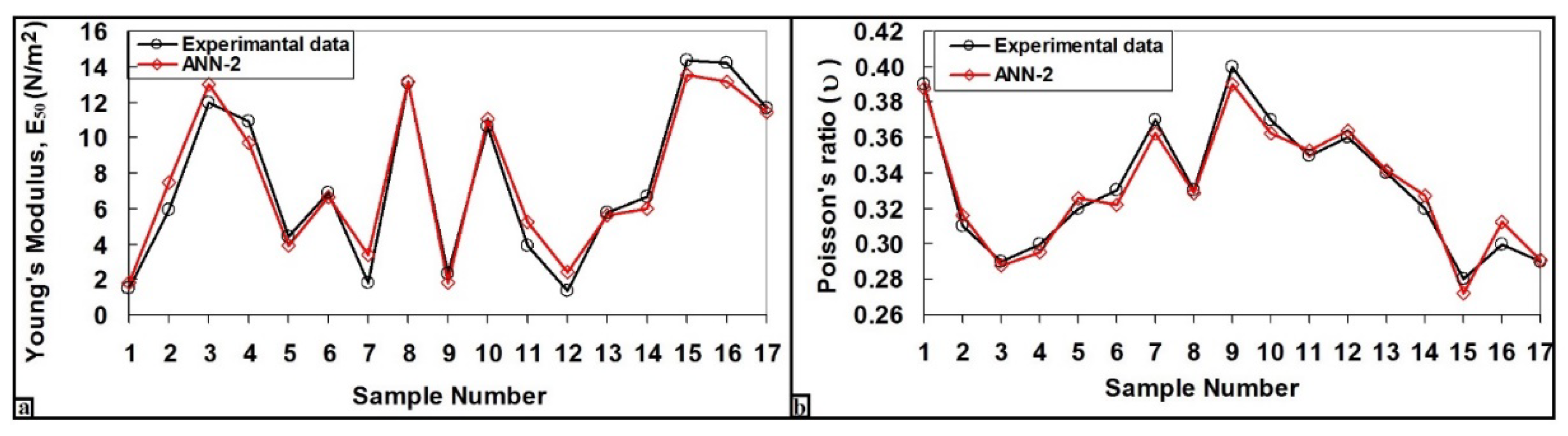

Table 1.
The materials used for the tests and their mineralogical properties.
| No | Description | Geological Origin |
Mineralogical Properties |
|---|---|---|---|
| 1 | Limestone-1 | Sedimentary | 50% clay contented |
| 2 | Limestone-2 | Sedimentary | very low porosity, sandy limestone texture |
| 3 | Limestone-3 | Sedimentary | micritic texture, fracture filling calcite and contains small amount of opaque minerals |
| 4 | Limestone-4 | Sedimentary | sparitic and homogeny texture |
| 5 | Siltstone | Sedimentary | contains 60% quartz |
| 6 | Green-Marl | Sedimentary | contains a small amount of silica |
| 7 | Gypsum | Sedimentary | less opaque and subhedral minerals |
| 8 | Barite | Sedimentary | 15% anhedral particle, be subject to tectonism, a hydrothermally deposited ore |
| 9 | Feldspar | Metamorphic | coarse crystalline albite mineral, contains 50% quartz minerals |
| 10 | Marble | Metamorphic | contains equidimensional and anhedral calcite crystals |
| 11 | Trass-1 | Igneous- Volcanic | contains amphibole, sanidine and biotite |
| 12 | Trass-2 | Igneous- Volcanic | contains 50% quartz minerals |
| 13 | Andesite-1 | Igneous- Volcanic | porphyritic, altered |
| 14 | Andesite-2 | Igneous- Volcanic | porphyritic, less altered |
| 15 | Galena | Mafic/ Ultramafic-Igneous ore | also contains pyrite and chalcopyrite |
| 16 | Sulphide ore | Mafic/ Ultramafic-Igneous ore | contains galena, pyrite, chalcopyrite and quartz |
| 17 | Chromite | Mafic/ Ultramafic-Igneous ore | contains 80% chromite, olivine and serpentine |
Table 2.
Statistical parameters of input and output variables.
| Test | Minimum | Maximum | Mean | Std. |
|---|---|---|---|---|
| E50 (N/m2) | 1.32 | 14.34 | 7.49 | 4.50 |
| υ | 0.28 | 0.40 | 0.33 | 0.04 |
| Vp (m/sec) | 1166 | 6697 | 4186 | 1440 |
| Vs (m/sec) | 652 | 2947 | 2090 | 608 |
| Vp/Vs | 1.78 | 2.40 | 1.97 | 0.19 |
| ρd (t/m3) | 2.00 | 2.94 | 2.45 | 0.07 |
| SH | 8.40 | 82.85 | 40.40 | 21.16 |
Table 3.
Details of the four ANN models according to the best input combinations.
| Model | Input Combination | Output | R2 | RMSE | MAE |
|---|---|---|---|---|---|
| ANN-1 | Vp, Vs, Vp/Vs, ρd, SH |
E50 (N/m2) υ |
0.891 0.961 |
1.490 0.007 |
0.947 0.005 |
| ANN-2 | Vp, Vs, Vp/Vs, SH |
E50 (N/m2) υ |
0.965 0.971 |
0.883 0.006 |
0.699 0.004 |
| ANN-3 | Vp, Vs, ρd, SH |
E50 (N/m2) υ |
0.925 0.956 |
1.252 0.008 |
1.037 0.006 |
| ANN-4 | Vp, Vs, Vp/Vs, ρd |
E50 (N/m2) υ |
0.896 0.953 |
1.478 0.008 |
1.106 1.106 |
Disclaimer/Publisher’s Note: The statements, opinions and data contained in all publications are solely those of the individual author(s) and contributor(s) and not of MDPI and/or the editor(s). MDPI and/or the editor(s) disclaim responsibility for any injury to people or property resulting from any ideas, methods, instructions or products referred to in the content. |
© 2024 by the authors. Licensee MDPI, Basel, Switzerland. This article is an open access article distributed under the terms and conditions of the Creative Commons Attribution (CC BY) license (http://creativecommons.org/licenses/by/4.0/).
Copyright: This open access article is published under a Creative Commons CC BY 4.0 license, which permit the free download, distribution, and reuse, provided that the author and preprint are cited in any reuse.


