
Submitted:
07 May 2025
Posted:
08 May 2025
You are already at the latest version
Abstract
Proper Orthogonal Decomposition (POD) methods, which primarily rely on linear dimensionality reduction, often fail to capture critical features in complex nonlinear flows. Conversely, while clustering methods excel in nonlinear feature extraction, they are limited by instability in cluster center initialization and inefficiencies in modal sorting, thereby restricting their usability in reduced-order modeling (ROM). To address these challenges, this study introduces the Clustering-based Reduced-Order Model (C-POD), which integrates POD preprocessing to stabilize cluster center selection and employs an Entropy-Controlled Euclidean-to-Probability Mapping (ECEPM) technique to refine modal sorting. The efficacy of C-POD is demonstrated through applications to Burgers’ equation and a cylinder wake flow case. Numerical results reveal that C-POD achieves superior dimensionality reduction accuracy compared to POD, with primary modes capturing more of the time-dependent dynamics and higher-order modes exhibiting enhanced physical interpretability. Moreover, ECEPM-based low-order modes significantly improve C-POD’ s accuracy in low-dimensional representations. The method’s low-order accuracy advantage is further substantiated through an inverse problem, where sparse sensor data enable the real-time reconstruction of the cylinder wake vorticity field. Results indicate that the Gappy C-POD method attains a 19.75% improvement in reconstruction accuracy and a 13.4% enhancement in the lower bound of reconstruction capability relative to Gappy POD. Additionally, C-POD maintains high reconstruction accuracy even at higher modal orders, making it particularly well-suited for reconstructing complex nonlinear system fields. This study offers compelling evidence supporting the potential application of the clustering-based C-POD framework to complex flow problems, thereby providing new insights into reduced-order modeling of nonlinear systems.
Keywords:
POD (Proper Orthogonal Decomposition)
; Clustering-based Reduced-Order Model Initialized by POD (C-POD)
; Reduced-Order Modeling (ROM)
; Nonlinear Model Order Reduction (NMOR)
1. Introduction
Efficient representation of high-dimensional spatiotemporal flow fields and the accurate capture of their dynamic evolution have long posed significant challenges in computational fluid dynamics (CFD). This is especially true for flow systems, such as cylinder wake flows [1,2], which exhibit both classical and complex behaviors. Although traditional CFD methods deliver high computational accuracy, their substantial computational costs and storage requirements severely limit their applicability in real-time prediction and optimization. To overcome these limitations, reduced-order models (ROMs) [3,4] provide a computationally efficient framework by constructing low-dimensional embedded spaces that extract dominant flow modes, thereby offering a robust paradigm for flow field reconstruction and predictive modeling. The fundamental strength of ROMs lies in establishing an accurate and robust mapping between high-dimensional dynamical systems and their low-dimensional surrogate models—a challenge that extends well beyond simple dimensionality reduction to encompass a deeper investigation of the fundamental dynamical structures governing fluid flow.
Traditional research on reduced-order models (ROMs) primarily focuses on control equations and can be broadly classified into three approaches: (1) modal decomposition projection methods (e.g., POD-Galerkin [5]), which construct low-dimensional subspaces by extracting dominant modes and then project the governing equations onto these subspaces; (2) balanced truncation methods [6], which utilize system controllability and observability analyses to retain the most significant state variables responsible for the input–output behavior; and (3) harmonic balance methods [7], which are employed for periodic flow problems by approximating steady-state solutions in the frequency domain using a finite set of Fourier basis functions. These methods offer several notable advantages. First, the reduction process is intimately linked with the physical structure of the underlying equations, thereby ensuring the mathematical interpretability of the model. Second, energy-optimal modal selection criteria, as exemplified by POD, facilitate the high-fidelity reconstruction of steady or weakly unsteady flow fields. However, these approaches also exhibit certain limitations. The assumption of a linear subspace may not adequately capture the multi-scale nonlinear dynamics inherent in turbulent flows. Additionally, in high Reynolds number regimes, the cumulative effect of modal truncation errors can precipitate instability in long-term predictions. Finally, the Galerkin projection relies on precise numerical integration and the orthogonality of basis functions, which may restrict its applicability in scenarios involving complex geometries and unstructured grids.
The rise of data-driven reduced-order models in recent years marks a shift in the direction of reduced-order modeling research. The technical framework of data-driven methods can be categorized into the following three main directions: (1) Data-driven modal methods, represented by snapshot POD [8], Dynamic Mode Decomposition (DMD)[9], and their variants. These methods extract spatiotemporal coherent structures from flow field data, eliminating the dependence on explicit control equations. By extracting principal components or modes from high-dimensional data, they effectively reduce computational dimensions while retaining the main dynamic features of the system. The key advantage is that these methods do not rely on complex physical models and equations, making them suitable for real-time applications in flow field reconstruction and prediction. However, these methods are highly dependent on large volumes of high-quality data and are sensitive to noise. In the case of complex nonlinear flows or strong disturbances, they may fail to capture flow details accurately, especially when flow conditions change, and the stability and transferability of the modes may be challenged. (2) Neural network-based nonlinear reduced-order methods, represented by autoencoders [10] and their various derivatives [11]. These methods train neural networks to learn the mapping between low-dimensional latent variables and high-dimensional variables in flow field data, effectively addressing highly nonlinear flow problems. Their strength lies in their powerful nonlinear fitting ability, enabling them to capture complex flow behaviors without relying on physical equations, especially excelling in nonlinear and time-varying flow fields. However, the limitations are also significant, particularly during model training, which requires large amounts of labeled data and computational resources, and may suffer from overfitting. Moreover, the "black-box" nature of neural networks makes them difficult to interpret and validate, limiting their application in scientific research, particularly in engineering problems requiring high physical interpretability. (3) Hybrid data-driven modeling methods, such as combining POD with machine learning regression models [12] (e.g., POD-RBF, POD-LSTM) or Physics-Informed Neural Networks (PINN) [13,14], aim to establish nonlinear mappings between low-dimensional latent variables through data training. These methods integrate traditional reduced-order techniques with advanced machine learning models, improving the adaptability of models to complex flow patterns while retaining physical information. The advantage of hybrid methods lies in their ability to enhance prediction accuracy while leveraging machine learning models to handle nonlinear and time-varying flow features, maintaining high physical interpretability. However, hybrid methods may encounter higher computational costs and model complexity during training and implementation, and require careful design of the hybrid model structure and optimization algorithms to ensure robustness and generalization ability.
Data-driven modal methods, represented by snapshot POD [8], not only offer dimensionality reduction and feature extraction capabilities but also exhibit strong mode resolution and excellent algorithm compatibility, making them widely applicable in the field of fluid mechanics [15]. However, these methods primarily rely on linear techniques to extract flow modes, which limits their effectiveness in handling strong nonlinear dynamic behaviors. For instance, POD may fail to fully capture nonlinear features in certain flow phenomena, such as the complex vortex interactions in turbulence, leading to extracted modes that do not accurately reflect the complexity of the flow. In contrast, clustering methods classify data based on data similarity, without being restricted to linear relationships, thus offering significant potential for improving the nonlinear dimensionality reduction capability of snapshot POD methods. Burkardt, J [16] and others were the first to propose a clustering-based approach for reduced-order modeling, the CVTs method (Centroid Voronoi Tessellation), demonstrating its effective application in incompressible flow problems. However, Burkardt, J did not distinguish the importance of modes derived from the CVT-based reduced-order model, limiting the ability to further extract dominant flow forms. Moreover, Burkardt, J pointed out that the selection of initial clustering centers significantly affects the accuracy of reduced-order models. He employed a hybrid approach using h-means and k-means clustering to select initial clustering centers. However, due to the randomness in clustering centers, the results can vary each time the reduced-order model is applied. To address the determination of initial clustering centers, Iqbal, M. M [17] introduced the Modified Pole Clustering (MPC) method, aimed at avoiding potential instability issues associated with pole clustering. However, the clustering-based reduced-order strategy proposed by Iqbal, M. M is more focused on the clustering process than the reduction modeling itself. He extracted clustering centers from the dataset and used nonlinear fitting to obtain pre-coefficients for these centers (approximated as modal coefficients), yielding a one-dimensional reduced-order model. However, as it did not use dataset projection to obtain modal coefficients, this approach fails to achieve effective modal decomposition and extraction. Huera-Huarte, F. J [18] and D'Adamo, J [19] combined clustering methods with POD in both simulations and experiments, using POD’s modal decomposition ability and the nonlinear feature extraction capability of clustering to analyze various vortex structures in the wake of a cylinder. However, they did not directly use the clustering centers obtained through clustering as orthogonal bases, instead applying a mean clustering method to cluster POD modal coefficients and reclassify the features extracted by POD. Wei, Z [20] proposed a new clustering-based reduced-order model, CROM. After clustering, CROM constructs a state transition matrix (CTM) to describe the transition probabilities between different flow states, with the state transition matrix serving to differentiate modal energies. This method enhances the model’s capability to extract nonlinear features while distinguishing modal energy levels, aiding in capturing the dynamic evolution of the flow. However, the state transition matrix in CROM is a high-dimensional probability matrix, and as the number of clustering centers increases, the matrix’s dimensionality grows sharply, limiting its application to high-dimensional complex flow problems. Moreover, when flow states change more delicately or multiple flow states exist, the matrix elements may become sparse, with some transition probabilities approaching zero, thereby diminishing the reliability and effectiveness of the model.
Previous developments in clustering-based reduced-order models have indicated that the stability of initial clustering centers and the modal ordering method are two critical factors limiting their practical implementation. In this paper, we propose a POD-initialized, mean clustering-based reduced-order model (C-POD ROM) that not only enhances the stability of initial clustering centers but also improves nonlinear dimensionality reduction capabilities. Moreover, we introduce a rapid and efficient modal sorting method, ECEPM, which enables C-POD ROM to effectively discriminate the contributions of different modes. The accuracy and modal extraction performance of C-POD ROM are initially validated by comparison with the snapshot POD method using the canonical one-dimensional Burgers equation. Subsequently, the interpretability of the modes sorted by ECEPM is examined in the context of a two-dimensional cylinder wake flow problem. Finally, leveraging the reduced-order characteristics of C-POD ROM, we explore its advantages in addressing an inverse problem—field reconstruction using sparse sensors. The paper is organized as follows: Section 2 introduces C-POD ROM and its modal sorting method; Section 3 presents an initial comparison of the dimensionality reduction capability of C-POD ROM using the one-dimensional Burgers equation; Section 4 validates the interpretability of the sorted modes using a two-dimensional cylinder wake flow case; and Section 5 discusses the application of C-POD ROM in inverse problem field reconstruction and presents preliminary verification results.
2. C-POD ROM and Modal Sorting Method
2.1. C-POD ROM
The Proper Orthogonal Decomposition (POD) method, based on Singular Value Decomposition (SVD), is a well-established, data-driven model reduction technique. POD generates a set of orthogonal basis functions that encapsulate the dominant features of a system. By employing linear combinations of these selected basis functions, one can effectively approximate the original system, thereby transforming a high-dimensional problem into a low-dimensional representation. To preserve computational resources, the snapshot POD method proposed by Sirovich is frequently used for dimensionality reduction of the dataset [21]. However, POD is inherently a linear reduction technique. Although it captures the primary dynamic features of linear systems, it may not fully represent the complexities of nonlinear flows, particularly when nonlinear behaviors vary across multiple time steps and spatial domains. In such cases, the low-rank approximation afforded by POD might not sufficiently capture these nonlinear effects.
Clustering methods exhibit robust capabilities in extracting nonlinear features, effectively capturing patterns and regularities in data, especially within complex nonlinear systems. Moreover, these methods can autonomously adapt to diverse data patterns, mapping both linear and nonlinear datasets into a low-dimensional space that elucidates underlying dynamic characteristics. Consequently, this paper integrates clustering concepts with model reduction techniques by proposing a clustering-based reduced-order modeling framework—C-POD ROM—to enhance the effectiveness of Proper Orthogonal Decomposition (POD) in addressing nonlinear model reduction challenges. The construction process is detailed as follows:
- (1)
- Arrange the responses of m data points under n different operating conditions as columns to form the database matrix D:
Here, dᵢ ∈ Rᵐ (i = 1,2,...,n) represents the data snapshot under the i-th operating condition.
- (2)
- Determining Initial Cluster Centers Based on the Snapshot POD Method [21]. First, the correlation matrix of the snapshot matrix D is constructed:
Solving the Eigenvalue Problem of the Correlation Matrix C:
Here, λᵢ represents the eigenvalue, and φᵢ is the corresponding eigenvector. The eigenvalues are arranged in descending order:
The corresponding eigenvectors φᵢ form an orthogonal basis, and the first K eigenvectors are selected as the initial cluster centers:
- (3)
- Sample Assignment. Each column vector dⱼ (j = 1, 2, ..., n) from the data matrix D is assigned to the nearest cluster center, forming K clusters:
Here, Sᵢ⁽ᵗ⁾ represents the number of vectors in the i cluster, μi denotes the i-th cluster centroid, t is the current iteration count, and ||·|| represents the Euclidean distance norm.
- (4)
- >4) Updating the Cluster Centers. The cluster centers are updated by calculating the mean of all vectors in each cluster Sᵢ, and this mean becomes the new cluster centroid:
- (5)
- Repeat steps (6) and (7) until the following convergence criterion is met:
- (6)
- To obtain the modal coefficients, project the original data matrix D onto the cluster bases μ by solving the following least squares problem [22]:
Here, aᵣ ∈ Rᵏ is the modal coefficient vector corresponding to the r-th snapshot, and the full data reconstruction expression is:
where A = [a₁ a₂ ... aₙ] ∈ Rᵏˣⁿ is the modal coefficient matrix, and D̂ is the reconstructed data matrix. Through the C-POD ROM, the database matrix D is decomposed into low-dimensional clustering basesand the modal coefficient matrix A.
2.2. Entropy-Controlled Euclidean-to-Probability Mapping Modal Sorting Method
One notable advantage of the POD method is its capacity to quantify the contribution of each mode to the reconstruction of the original data. This contribution is indicated by the singular values, which represent the projection strength of the original data matrix onto the orthogonal modes. Larger singular values imply a more significant contribution from the corresponding mode in reconstructing the data, thereby identifying it as a dominant mode that captures the primary operational characteristics of the system. In contrast, the Clustering-based POD Reduced-Order Model (C-POD ROM) does not involve singular value decomposition during its construction, rendering it infeasible to assess mode contributions based on singular value magnitudes. In this context, the modes derived from the modal coefficient matrix obtained via C-POD ROM are considered unordered, lacking a definitive hierarchy in terms of their importance in the model reduction process. To equip clustering-based reduced-order models with the capacity to differentiate mode contributions in a manner analogous to the POD method, this paper introduces an Entropy-Controlled Euclidean-Probability Mapping (ECEPM) approach. This method ranks the contribution levels of clustering bases obtained through C-POD ROM by computing the entropy and Euclidean distance for each mode, subsequently converting these metrics into probability values. This ranking methodology is analogous to mode energy sorting based on singular values in the POD method, thereby ensuring effective feature extraction and mode separation within C-POD ROM.
- (1)
- Euclidean Distance Matrix Construction: Assume the database matrix , Clustering bases , The column vectors are , , where,
- (2)
- Compute the column-wise sum of squares for and as shown in Equations (11) and (12).
- (3)
- Construct the inner product matrix G
- (4)
- Construct the squared Euclidean distance matrix
where 1 is a matrix with all elements equal to 1, so the Euclidean distance matrix is:
Probability Mapping Function Construction: After obtaining the Euclidean distance matrix , the goal is to transform it into a weight probability mapping matrix , where represents the probability value of the i-th clustering base for the j-th sample. A higher probability value indicates a greater contribution of that clustering base to the current sample value, while satisfying .
- (1)
- Take the negative of the distance matrix C and shift each column, to avoid overflow in exponential calculations, resulting in the matrix Z:
where , , represent the outer product.
- (2)
- Perform the exponential operation on the shifted matrix and introduce the temperature parameter
, resulting in:
- (3)
- Normalize the exponential matrix column-wise to obtain the final probability weight matrix W:
where: represents element-wise division, is the sum of each column, and extends the column sum to a matrix where all columns are identical. In the construction of the probability mapping function, the temperature parameter is used to adjust the entropy of the probability distribution. When , the probability distribution tends to be uniform, with similar contributions from each mode. When , the distribution skews toward modes with higher contribution, and the probabilities of other modes become smaller. To ensure the rationality of the probability mapping matrix, we set in this study.
Through the above entropy-controlled Euclidean-to-probability mapping method, the probability weight matrix W is obtained. For different samples in the database matrix, represents the probability value of the i-th clustering base for the j-th sample. A higher probability value indicates a greater contribution of that clustering base to the current sample value. Therefore, by examining the values in W, the importance of each clustering base in the C-POD ROM is distinguished. The construction process of the C-POD ROM and the entropy-controlled Euclidean-to-probability mapping method is shown in Figure 1. In Section 3 and Section 4, to validate the effectiveness of the C-POD ROM method, we apply it to two classic fluid dynamics problems: the one-dimensional Burgers equation and the two-dimensional cylinder wake flow. These problems exhibit distinct nonlinear characteristics, making them ideal for testing the practical applicability of the method.
3. Burgers’ Equation and C-POD ROM
3.1. Introduction to the One-Dimensional Burgers' Equation
As a nonlinear partial differential equation, the Burgers' equation holds significant research value across various domains, including fluid mechanics [23] and meteorological forecasting [24]. In addition to characterizing the propagation of nonlinear waves, it encapsulates essential physical phenomena, such as viscosity and diffusion. Its inherent nonlinearity facilitates the simulation of complex flow phenomena, particularly in convection-dominated fields where highly nonlinear behaviors are prevalent. Reduced-order models aim to minimize computational costs while preserving the fundamental characteristics of the system. Consequently, using the Burgers' equation as a test case provides an effective means to evaluate the efficacy and accuracy of these models in addressing nonlinear and transient flow processes. In this study, the accuracy of the Proper Orthogonal Decomposition (POD) and Complexified POD (C-POD) reduced-order models is comparatively assessed using a one-dimensional Burgers' equation as the benchmark case. The mathematical formulation of the Burgers' equation is presented as follows:
Let u(x, t) denote the wave amplitude, c represent the wave speed (i.e., the coefficient of the convection term), and β denote the dissipation coefficient. The one-dimensional Burgers’ equation incorporates both convection and diffusion characteristics, reflecting aspects of the heat conduction equation and the Navier-Stokes equations. Consequently, it establishes a conceptual link to both heat conduction and convection phenomena.
Consider the initial condition in the form of a Gaussian pulse, as shown in Equation (20):
Under this initial condition, the analytical solution to the one-dimensional Burgers' equation is given by [25]:
Here, x₀ denotes the initial peak position of the wave, σ represents the width of the wave packet, and c is the propagation speed (consistent with the meaning and value specified in Equation (19)). The analytical solution describes a Gaussian wave packet propagating in the x-direction with velocity c. Notably, the width of the wave packet increases gradually over time, indicative of a diffusion phenomenon, while its amplitude decreases, reflecting a dissipation phenomenon that leads to gradual attenuation during propagation. A schematic illustration of the wave evolution in the one-dimensional Burgers' equation is presented in Figure 2.
3.2. Database Construction
To evaluate the performance of the POD and C-POD reduced-order models, a dataset based on the Burgers' equation is first constructed. The initial conditions and parameters are set as follows:
Initial Conditions:
Initial wave peak position: x0=0
Initial wave packet width: σ=1
Spatial and Temporal Discretization:
Spatial range: x∈[0,10], with Nx=1000 uniformly distributed sampling points
Temporal range: t ∈ [0,5], with waveforms sampled at intervals of Δt=0.5
Independent Variable Settings:
Wave speed c range: c∈ [0.1,2]
Dissipation coefficient β range: β∈ [0,1]
Based on these settings, a database D1 is constructed with independent variable combinations: c∈{0.1,0.5,1,1.5,2}、β∈{0,0.2,0.4,0.6,0.8,1}
Consequently, the size of the database matrix D1 is 1000×303 (i.e., 1000 spatial points combined with 303 independent variable combinations).
3.3. C-POD ROM Accuracy Testing and Modal Decomposition
To evaluate the performance of the POD and C-POD reduced-order methods, we performed order reduction on the dataset and reconstructed the original data using various modal orders. The correlation coefficient and root mean square error (RMSE) were employed as assessment metrics. Furthermore, a novel metric, Cr, defined in Equation (22), was introduced to comprehensively evaluate the accuracy of the reduced-order models.
where the root mean square error (RMSE) and the Pearson correlation coefficient r are defined as shown in Equations (23) and (24):
where: n is the number of data points; is the actual value; is the predicted value; is the mean of the actual data and is the mean of the predicted data. A higher Cr value indicates an increasing trend in RMSE or a decreasing trend in the correlation coefficient, suggesting poorer reduced-order modeling performance.
Under varying levels of modal truncation, the datasets were reduced using both the POD and C-POD methods. The resulting modal coefficients and orthogonal bases were then employed to reconstruct the original datasets. Figure 3 and Figure 4 present the average and maximum values of Cr, computed using Equation (22). The average Cr value reflects the overall reduction capability, while the maximum value indicates the lower bound of this capability. As illustrated in Figure 3, both methods exhibit enhanced reduction performance with increasing modal truncation, stabilizing at higher modal orders. For modal orders below 6, the reduction capabilities of the two methods are comparable; however, for order values above this threshold, the C-POD method significantly outperforms POD. Figure 4 further shows that, regarding the lower bound of reduction capabilities, C-POD is superior at modal orders 7, 8, and 9, whereas POD maintains an advantage at other modal orders. These findings preliminarily highlight the superior reduction accuracy of the C-POD method.
To compare the modal extraction capabilities of the C-POD and POD methods, we analyzed the reduced-order modeling of the Burgers' equation under the following conditions: c=0.1, β=0.2, and c=2, β=1. At times t=0, 1, and 2 seconds, both methods were applied for model reduction, and the time evolution of the first-order mode (dominant mode) was obtained using the ECEPM method, as shown in Figure 5 and Figure 6. As observed from Figure 5 and Figure 6, the first-order modes derived from the C-POD reduced-order model effectively capture the temporal evolution of the waveform, including the reduction in peak amplitude and the propagation of the waveform along the positive x-axis over time. In contrast, the first-order modes obtained using the POD method exhibit minimal temporal variation, failing to capture the dynamic trends and characteristics of the waveform over time. A further comparison reveals that, for the first-order modes extracted by the C-POD method, the rate of decrease in peak amplitude over time is positively correlated with the value of β, while the distance of waveform propagation along the positive x-axis correlates positively with the wave speed c. These findings preliminarily suggest that, compared to the POD method, the dominant modes obtained via the C-POD method encapsulate more of the system's temporal evolutionary characteristics.
4. Cylinder Wake Flow Case Introduction
Two-dimensional flow around a cylinder represents a classical complex flow problem in fluid dynamics, characterized by phenomena such as vortex shedding, flow separation, and turbulence. In contrast to the one-dimensional Burgers' equation, this flow configuration exhibits more intricate turbulent features, revealing a rich spectrum of physical phenomena. Consequently, it serves as an excellent benchmark for validating the efficacy of reduced-order models in capturing complex flow dynamics.
4.1. Model Introduction
To simulate two-dimensional fluid flow around a cylinder, the computational domain is configured as a rectangular region with the cylinder positioned near the mid-left boundary. The cylinder has a radius of 5 mm, and the domain dimensions are Lx = 1 mm (length) and Ly = 40 mm (width). Inflow velocities at the left boundary are varied to adjust the Reynolds number (Re), thereby capturing a range of flow phenomena. Figure 7 illustrates the geometric configuration of the computational domain.
For the two-dimensional incompressible Navier-Stokes equations, the motion of the fluid is described by the following equations:
where u=(u, v) represents the velocity field components, with u being the velocity in the x direction and v is the velocity in the y direction; p is the pressure field; ν is the fluid’s kinematic viscosity; and f represents the body force (in this case, the body force field).For this two-dimensional flow problem, the governing equations are discretized using the finite difference method, and the implicit method combined with the Alternating Direction Implicit (ADI) method is used for time-stepping solutions. The specific solution process is briefly described below:
- (1)
- Using the Alternating Direction Implicit (ADI) method, the equation is split into two one-dimensional equations. The implicit solution is first performed in the x direction, followed by the implicit solution in the y direction:
- (2)
- The pressure field is obtained by solving the Poisson equation using the Fast Fourier Transform (FFT):
- (3)
- Set a fixed flow velocity at the left boundary x=0, and apply a no-slip boundary condition on the surface of the cylinder.
- (4)
- To quantify the rotational behavior in the flow field around the cylinder, the calculation of vorticity is introduced in the two-dimensional incompressible flow field. The vorticity is defined as:
The vorticity field distribution is obtained through the differential method as follows:
4.2. Grid Independence and Numerical Method Validation
To validate the reliability of the numerical method and the grid used in this study, we first perform a computational model verification for a fixed single cylinder with Re=100. The effects of total grid number and dimensionless time step on the results are considered, and the results are compared with the Stanton number and Lift coefficient values obtained from the literature [26,27,28]. The comparison results are presented in Table 1. The dimensionless time step is defined as shown in Equation (32):
where represents the time step, is the upstream inlet velocity of the cylinder, and is the diameter of the cylinder.
From Table 1, it can be observed that the simulation results remain consistent as the grid number increases from 400×160 to 800×320. When the dimensionless time step is less than or equal to 0.01, the results are in close agreement with those in the literature. Therefore, in this study, we choose the A3 condition, setting the total grid number to 400×160 and the dimensionless time step to 0.01.
4.3. Presentation of Computational Results
Figure 8 presents the vorticity distribution corresponding to several typical flow state transitions in the two-dimensional flow around a cylinder at Re = 150. The specific flow states are detailed as follows:
- (1)
- From t=1 to 9 seconds, a pair of side vortices form on either side of the cylinder, gradually creating a pair of vortices with opposite rotational directions behind the cylinder.
- (2)
- From t=9 to 33 seconds, the counter-rotating vortices behind the cylinder gradually move and diffuse in the direction of the flow.
- (3)
- From t=33 to 110 seconds, the counter-rotating vortices behind the cylinder disappear, and the flow becomes more stable.
- (4)
- For times exceeding 110 seconds, the flow pattern undergoes notable changes, with vortices detaching periodically to form a stable vortex street. Multiple regions of alternating positive and negative vorticity emerge, indicating pronounced shear and recirculation phenomena within the flow field-hallmarks of the classic Kármán vortex street.
4.4. Cylinder Wake Flow Field Dimensionality Reduction and Reconstruction Accuracy, and Modal Decomposition
4.4.1. Dataset and Test Set Construction
To test the accuracy variations of POD and C-POD in the reduced-order modeling and reconstruction of vorticity fields in flow around a cylinder, as well as their modal decomposition capabilities for the flow behavior of the cylinder, a database was constructed over the entire evolution of the cylinder's flow pattern at Re = 150. Specifically, the time range was set from t=0 to 145 seconds, with data collected every 0.1 seconds. The vorticity field distribution data were then written into the dataset, resulting in a total database size of 64000×1450.
4.4.2. Dimensionality Reduction and Reconstruction Accuracy of Cylinder Wake Flow Field
This section assesses the accuracy of the Proper Orthogonal Decomposition (POD) and Constrained-POD (C-POD) reduced-order models (ROMs) in both the dimensionality reduction and reconstruction of the cylinder wake vorticity field, as well as their modal decomposition capabilities for characterizing the cylinder's wake flow behavior. As illustrated in Figure 9, the average Cr value of C-POD is higher at lower modal orders; however, as the modal order increases, the average Cr value of C-POD decreases rapidly and eventually stabilizes at values consistently lower than those observed for POD. At higher modal orders, C-POD maintains a lower average Cr value, indicating improved reconstruction accuracy across multiple modes relative to POD. Furthermore, as shown in Figure 10, C-POD exhibits a lower maximum Cr value when managing higher modal orders compared to POD, suggesting a distinct advantage in minimizing the worst-case reconstruction error. Overall, C-POD demonstrates superior performance in terms of dimensionality reduction model accuracy-both in the lower bound of capability (maximum Cr) and the overall average accuracy (mean Cr)—thereby confirming its enhanced dimensionality reduction capability over that of POD.
4.4.3. Comparison of Modal Decomposition Results
Based on Figure 9, the first 10 modal orders are selected, and the POD and C-POD methods are used to decompose the vorticity field of the cylinder wake at t=236 seconds and t=240 seconds under the condition of Re=150, when the flow transitions into a stable vortex street. The vorticity field dominated by the first six modal orders is shown in Figure 11 and Figure 12. From the comparison of Figure 11 and Figure 12, it can be observed that the vorticity field dominated by the first six modes extracted by C-POD mainly contains four types of vortical structures, as shown in Figure 13. These are named as:
- (1)
- Type 1 vortex: Symmetrical side vortices extending downstream from both sides of the cylinder into the flow region.
- (2)
- Type 2 vortex: Counter-rotating pair of vortices formed at the rear of the cylinder due to recirculation, resembling a "horseshoe" shape.
- (3)
- Type 3 vortex: Developing horseshoe-shaped vortices.
- (4)
- Type 4 vortex: Asymmetric side vortices on both sides of the cylinder.
Between t = 236 seconds and t = 240 seconds, vortex formation in the vorticity field is characterized by changes in the 1st, 2nd, and 5th modal orders, with all vortices exhibiting a contraction trend toward the rear of the cylinder. Concurrently, the rotational direction of vortices in the 1st, 3rd, 5th, and 6th modal orders reverses. Lower-order POD modes correspond to the primary flow structures and are thus more intuitively interpretable. However, as the modal order increases, modes such as the 2nd and 3rd capture more complex flow characteristics, including primary vortices, secondary vortices, and localized vortices. Despite this, the physical interpretation of vortex evolution—particularly the temporal dynamics of higher-order modes—remains a challenging endeavor.
To further validate the reliability of the ECEPM method in ranking the significance of the basis for C-POD ROM clustering, the total number of modes is set to 10. The ECEPM method selects the first n modes, reconstructing the vorticity field distributions at t = 236 seconds and t = 240 seconds while computing the corresponding Cr values. These results are then compared with those obtained using the POD method, as shown in Figure 14. Figure 14 illustrates that when the modal order is less than three, the reconstruction accuracy of the C-POD method increases rapidly with additional modes, exhibiting a significantly greater improvement than the POD method. This finding suggests that the first n modes selected by the ECEPM method promptly capture the system's primary features, and the C-POD method demonstrates robust reconstruction capabilities at lower modal orders. However, as the modal order increases further, the reconstruction accuracies of both methods tend to converge.
4.5. Evolutionary Characteristics of Modes Extracted by C-POD over Time
To further investigate the temporal evolution of modes extracted by C-POD, Figure 15 plots the variation of the first and second modal coefficients over time. The vorticity values in the cloud plot are restricted to the range [-2, 2] to facilitate comparison. Evidently, the modal coefficients for both the first and second modes exhibit inflection points not only at the primary transition moments of the flow states (t = 1 s, 9 s, 33 s, 110 s) but also at t = 5 s, 13.5 s, 22 s, and 119.5 s. This finding indicates that the time-varying modal coefficients of the C-POD reduced-order model capture both the predominant flow feature transitions in the cylinder wake and more subtle flow variations. Figure 16, Figure 17 and Figure 18 illustrate the variations in the vorticity field dominated by the first and second modes of the C-POD ROM at t = 1 s, 5 s, 9 s, 13.5 s, 22 s, 33 s, 110 s, and 119.5 s. For t < 9 s, the vorticity field associated with the first mode primarily comprises the third-type vortex, whose intensity decreases over time, thereby diminishing its influence on the overall field. Concurrently, the second-mode vorticity field transitions gradually from an irregular fourth-type vortex to a first-type vortex, with the direction of rotation altering at t = 1 s, 5 s, and 9 s. For 9 s < t < 14.5 s, the vorticity field governed by the first mode evolves from a third-type to a first-type vortex, and its influence progressively extends throughout the entire flow field. Between 13.5 s and 33 s, the vorticity field distribution stabilizes, accompanied by a change in the rotation direction for the second mode. For 33 s < t < 110 s, the vorticity field attains a stable state, with negligible changes in the vortex structures and vorticity values corresponding to both the first and second modes. During the interval from 110 s to 119.5 s, the system transitions toward a stable vortex street formation; notably, the elongated side vortices on both sides of the cylinder become unstable and commence vortex shedding at the tail, while the rotation direction in the second-mode vorticity field undergoes further alteration. For t > 119.5 s, the system enters a state of stable vortex street generation, and as depicted in Figure 15, the coefficients corresponding to the first and second modes exhibit a periodic oscillatory trend over time.
5. Application Value of C-POD ROM in Inverse Problems
The Gappy POD method [29,30] is a derivative of the POD reduced-order model, primarily used to solve the full field reconstruction inverse problem when only sparse sensor data is available. The accuracy of this method heavily depends on the precision of the reduced-order model under low-order conditions. In both POD and C-POD methods, low-order modes represent the primary dynamics of the system, typically carrying most of the energy or important information, while high-order modes often represent finer details or noise. For a system, low-order modes are typically associated with the main frequencies and significant physical behaviors, making them more accurate for data reconstruction. Through the analysis in Section 5, we found that, in the cylinder wake problem, C-POD ROM has a greater advantage over POD ROM at lower modal orders. This low-order advantage should be better reflected in inverse problems based on reduced-order methods. Continuing with the cylinder wake case described in Section 4.4.3, we describe the performance of this inverse problem in the cylinder wake scenario as follows: placing a specified number of sparse sensors in the vorticity field of the cylinder wake, and reconstructing the vorticity field in real-time based only on the sparse sensor data, to capture the complete vortex evolution of the cylinder wake.
80% of the original dataset is randomly selected as the training set, and the remaining 20% is used as the validation set. Using the correlation coefficient filtering method proposed by Qingyang Yuan [31], 7 optimal sparse sensor locations are selected in the vorticity field behind the cylinder in the cylinder wake. These sparse sensors can output real-time vorticity information at their respective positions. Based on the sparse sensor data, the missing reconstruction methods based on POD reduced-order models (Gappy POD) and C-POD reduced-order models (Gappy C-POD) are used to reconstruct the cylinder wake flow field under different modal orders, and the reconstruction capabilities are measured, as shown in Figure 17 and Figure 18.
From Figure 19 and Figure 20, it is observed that the reconstruction accuracy of the Gappy POD method increases initially and then decreases as the modal order increases. When the modal order is 5, the Gappy POD method achieves its optimal reconstruction accuracy, with an average Cr value of 0.81 and a maximum Cr value of 0.97. When the modal order is less than 12, the reconstruction accuracy of the Gappy C-POD method follows a similar trend, increasing initially and then decreasing. When the modal order is 6, the average Cr value is 0.65 and the maximum Cr value is 0.84. However, when the modal order exceeds 12, the reconstruction accuracy of Gappy C-POD decreases as the modal order increases. When the modal order reaches 20, the average Cr value drops to 0.49, lower than the average value of 0.65 at modal order 6. This demonstrates the significant advantage of the Gappy C-POD method over the Gappy POD method in reconstructing inverse problems. The average reconstruction accuracy of Gappy C-POD is improved by 19.75% compared to Gappy POD, and the lower bound of reconstruction capability is improved by 13.4%. Furthermore, the Gappy C-POD method can achieve higher field reconstruction accuracy under higher modal order conditions, as higher modal orders can capture more complex flow behaviors. Therefore, the Gappy C-POD method is more suitable for field reconstruction in complex nonlinear systems.
Based on the above analysis, a modal order of 5 is chosen for the Gappy POD method and a modal order of 6 for the Gappy C-POD method. The reconstruction of the cylinder wake vorticity field at t=141 seconds is shown in Figure 21 and Figure 22. From left to right, the three images in Figure 21 and Figure 22 represent the cylinder wake vorticity field at t=141 seconds, the reconstructed field with sparse sensor layout, and the distribution of reconstruction relative error. From Figure 21 and Figure 22, it can be seen that the maximum error in the field reconstruction using the Gappy C-POD method is 25%, which is smaller than the maximum error of 35% in the field reconstruction using the Gappy POD method.
6. Conclusions
In this paper, we address the limitations of the proper orthogonal decomposition (POD) method in achieving robust linear dimensionality reduction by introducing a clustered POD (C-POD) reduced-order model. We assess the model's capabilities in both dimensionality reduction and reconstruction using the one-dimensional Burgers' equation and the two-dimensional cylinder wake problem. The proposed C-POD reduced-order model offers the following advantages:
- The C-POD reduced-order model leverages proper orthogonal decomposition to initialize clustering centers, while the proposed ECEPM method evaluates the modes within the C-POD ROM and ranks their importance. This approach effectively addresses two critical challenges in clustering-based reduced-order models: ensuring the stability of the initial clustering centers and establishing a robust mode ranking methodology.
- The C-POD ROM outperforms the POD in dimensionality reduction accuracy. Specifically, it exhibits superior performance in terms of both the lower bound of dimensionality reduction capability (maximum of Cr) and overall average accuracy (mean of Cr). Furthermore, compared to the POD, the dominant modes extracted by the C-POD ROM encapsulate a broader spectrum of the system’s temporal evolutionary features, and its higher-order modes offer enhanced physical interpretability.
- The advantage of low-order accuracy in the C-POD ROM is particularly evident in inverse problems employing reduced-order methods. Specifically, the missing data reconstruction approach based on the C-POD reduced-order model (Gappy C-POD) enhances the average reconstruction accuracy by 19.75% and increases the lower bound of reconstruction capability by 13.4% compared to the conventional Gappy POD method. Moreover, the Gappy C-POD technique achieves superior field reconstruction accuracy at higher modal orders, which are essential for capturing more intricate flow behaviors. Consequently, the Gappy C-POD method is especially well-suited for field reconstruction in complex nonlinear systems.
References
- Guo T, Wu W L, Luo Z M, et al. Mode transition and drag characteristics of non-circular cylinders in a uniform flow[J]. OCEAN ENGINEERING, 2024,297.
- Santana G M, Fabro A T, Miserda R. Analysis of the dynamic modes of the transonic flow around a cylinder[J]. JOURNAL OF THE BRAZILIAN SOCIETY OF MECHANICAL SCIENCES AND ENGINEERING, 2024,46(9).
- Copeland D M, Cheung S W, Huynh K, et al. Reduced order models for Lagrangian hydrodynamics[J]. COMPUTER METHODS IN APPLIED MECHANICS AND ENGINEERING, 2022,388.
- Knockaert L, De Zutter D. Stable Laguerre-SVD reduced-order modeling[J]. IEEE TRANSACTIONS ON CIRCUITS AND SYSTEMS I-FUNDAMENTAL THEORY AND APPLICATIONS, 2003,50(4):576-579.
- Couplet M, Basdevant C, Sagaut P. Calibrated reduced-order POD-Galerkin system for fluid flow modelling[J]. JOURNAL OF COMPUTATIONAL PHYSICS, 2005,207(1):192-220.
- Besselink B, van de Wouw N, Scherpen J, et al. Model Reduction for Nonlinear Systems by Incremental Balanced Truncation[J]. IEEE TRANSACTIONS ON AUTOMATIC CONTROL, 2014,59(10):2739-2753.
- Grolet A, Thouverez F. On a new harmonic selection technique for harmonic balance method[J]. MECHANICAL SYSTEMS AND SIGNAL PROCESSING, 2012,30:43-60.
- Bagheri M H, Esmailpour K, Hoseinalipour S M, et al. Numerical study and POD snapshot analysis of flow characteristics for pulsating turbulent opposing jets[J]. INTERNATIONAL JOURNAL OF NUMERICAL METHODS FOR HEAT & FLUID FLOW, 2019,29(6):2009-2031.
- Bistrian D A, Navon I M. Randomized dynamic mode decomposition for nonintrusive reduced order modelling[J]. INTERNATIONAL JOURNAL FOR NUMERICAL METHODS IN ENGINEERING, 2017,112(1):3-25.
- Phillips T, Heaney C E, Smith P N, et al. An autoencoder-based reduced-order model for eigenvalue problems with application to neutron diffusion[J]. INTERNATIONAL JOURNAL FOR NUMERICAL METHODS IN ENGINEERING, 2021,122(15):3780-3811.
- Zhang X S, Ji T W, Xie F F, et al. Data-driven nonlinear reduced-order modeling of unsteady fluid-structure interactions[J]. PHYSICS OF FLUIDS, 2022,34(5).
- Shen X W, Du C B, Jiang S Y, et al. Enhancing deep neural networks for multivariate uncertainty analysis of cracked structures by POD-RBF[J]. THEORETICAL AND APPLIED FRACTURE MECHANICS, 2023,125.
- Yuan L, Ni Y Q, Deng X Y, et al. A-PINN: Auxiliary physics informed neural networks for forward and inverse problems of nonlinear integro-differential equations[J]. JOURNAL OF COMPUTATIONAL PHYSICS, 2022,462.
- Taassob A, Kumar A, Gitushi K M, et al. A PINN-DeepONet framework for extracting turbulent combustion closure from multiscalar measurements[J]. COMPUTER METHODS IN APPLIED MECHANICS AND ENGINEERING, 2024,429.
- Bagheri M H, Esmailpour K, Hoseinalipour S M, et al. Numerical study and POD snapshot analysis of flow characteristics for pulsating turbulent opposing jets[J]. INTERNATIONAL JOURNAL OF NUMERICAL METHODS FOR HEAT & FLUID FLOW, 2019,29(6):2009-2031.
- Burkardt J, Gunzburger M, Lee H C. Centroidal Voronoi tessellation-based reduced-order modeling of complex systems[J]. SIAM JOURNAL ON SCIENTIFIC COMPUTING, 2006,28(2):459-484.
- Iqbal M M, Xavier R J. Development of optimal reduced-order model for gas turbine power plants using particle swarm optimization technique[J]. INTERNATIONAL TRANSACTIONS ON ELECTRICAL ENERGY SYSTEMS, 2020,30(4).
- Huera-Huarte F J, Vernet A. Vortex modes in the wake of an oscillating long flexible cylinder combining POD and fuzzy clustering[J]. EXPERIMENTS IN FLUIDS, 2010,48(6):999-1013.
- D'Adamo J, Collaud M, Sosa R, et al. Wake and aeroelasticity of a flexible pitching foil[J]. BIOINSPIRATION & BIOMIMETICS, 2022,17(4).
- Wei Z, Yang Z G, Xia C, et al. Cluster-based reduced-order modelling of the wake stabilization mechanism behind a twisted cylinder[J]. JOURNAL OF WIND ENGINEERING AND INDUSTRIAL AERODYNAMICS, 2017,171:288-303.
- Sirovich, L. Turbulence and the dynamics of coherent structures. I. Coherent structures. Quart Appl Math, 1987, 45(3): 561.
- Guo H B, Renaut R A. A regularized total least squares algorithm: TOTAL LEAST SQUARES AND ERRORS-IN-VARIABLES MODELING: ANALYSIS, ALGORITHMS AND APPLICATIONS[Z]. VanHuffel S, Lemmerling P. 3rd International Workshop on Total Least Squares and Errors-in-Variables Modeling: 200257-66.
- Yuan S L, Blömker D, Duan J Q. Stochastic turbulence for Burgers equation driven by cylindrical Levy process[J]. STOCHASTICS AND DYNAMICS, 2022,22(02).
- Li L, Ong K. Dynamic Transitions of Generalized Burgers Equation[J]. JOURNAL OF MATHEMATICAL FLUID MECHANICS, 2016,18(1):89-102.
- SENECHAL, M. SPATIAL TESSELLATIONS - CONCEPTS AND APPLICATIONS OF VORONOI DIAGRAMS - OKABE,A, BOOTS,B, SUGIHARA,K[J]. SCIENCE, 1993,260(5111):1170.
- WILLIAMSON, C. OBLIQUE AND PARALLEL MODES OF VORTEX SHEDDING IN THE WAKE OF A CIRCULAR-CYLINDER AT LOW REYNOLDS-NUMBERS[J]. JOURNAL OF FLUID MECHANICS, 1989,206:579-627.
- Singha S, Sinhamahapatra K P. High-Resolution Numerical Simulation of Low Reynolds Number Incompressible Flow About Two Cylinders in Tandem[J]. JOURNAL OF FLUIDS ENGINEERING-TRANSACTIONS OF THE ASME, 2010,132(1).
- Qu L X, Norberg C, Davidson L, et al. Quantitative numerical analysis of flow past a circular cylinder at Reynolds number between 50 and 200[J]. JOURNAL OF FLUIDS AND STRUCTURES, 2013,39:347-370.
- Everson R, Sirovich L. Karhunen–Loève procedure for gappy data. J Opt Soc Am A, 1995, 12(8): 1657.
- Deus, J. Martin, E. Efficient Cardiovascular Parameters Estimation for Fluid-Structure Simulations Using Gappy Proper Orthogonal Decomposition. Ann Biomed Eng 52, 3037–3052 (2024).
- Yuan Q, Guo X, Han J, et al. Correlation Coefficient Filtering Method for Optimal Sensor Layout Strategies in Inverse Problems[J]. Journal of Engineering, 2025,2025(1):5142118.
Figure 1.
Schematic Representation of the C-POD ROM Construction Process.
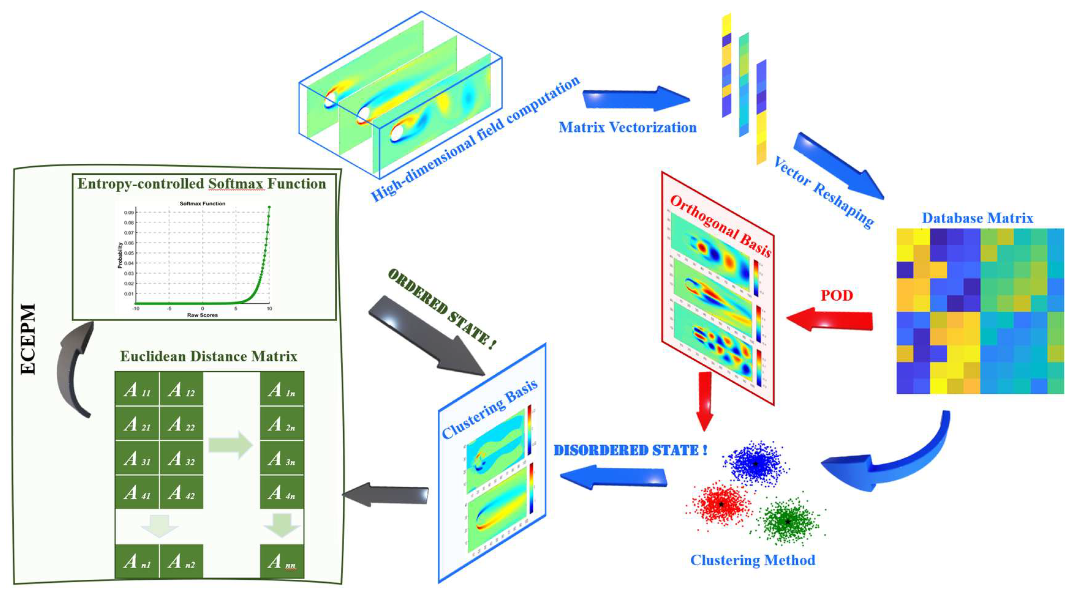
Figure 2.
Schematic of wave evolution in the one-dimensional Burgers' equation.
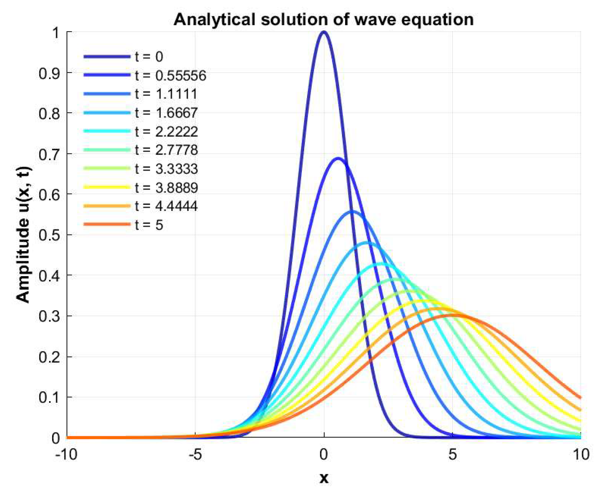
Figure 3.
Variation of the Average Cr Value with Respect to Different Modal Order Conditions.
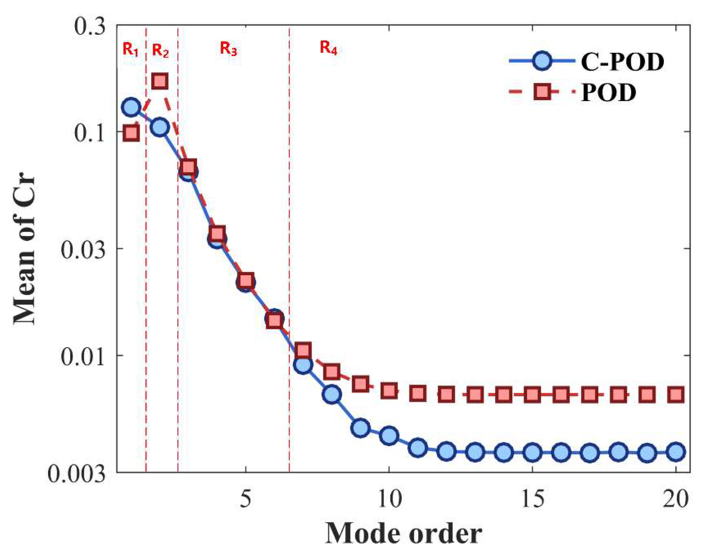
Figure 4.
Variation of the Average Cr Value with Respect to Different Modal Order Conditions.
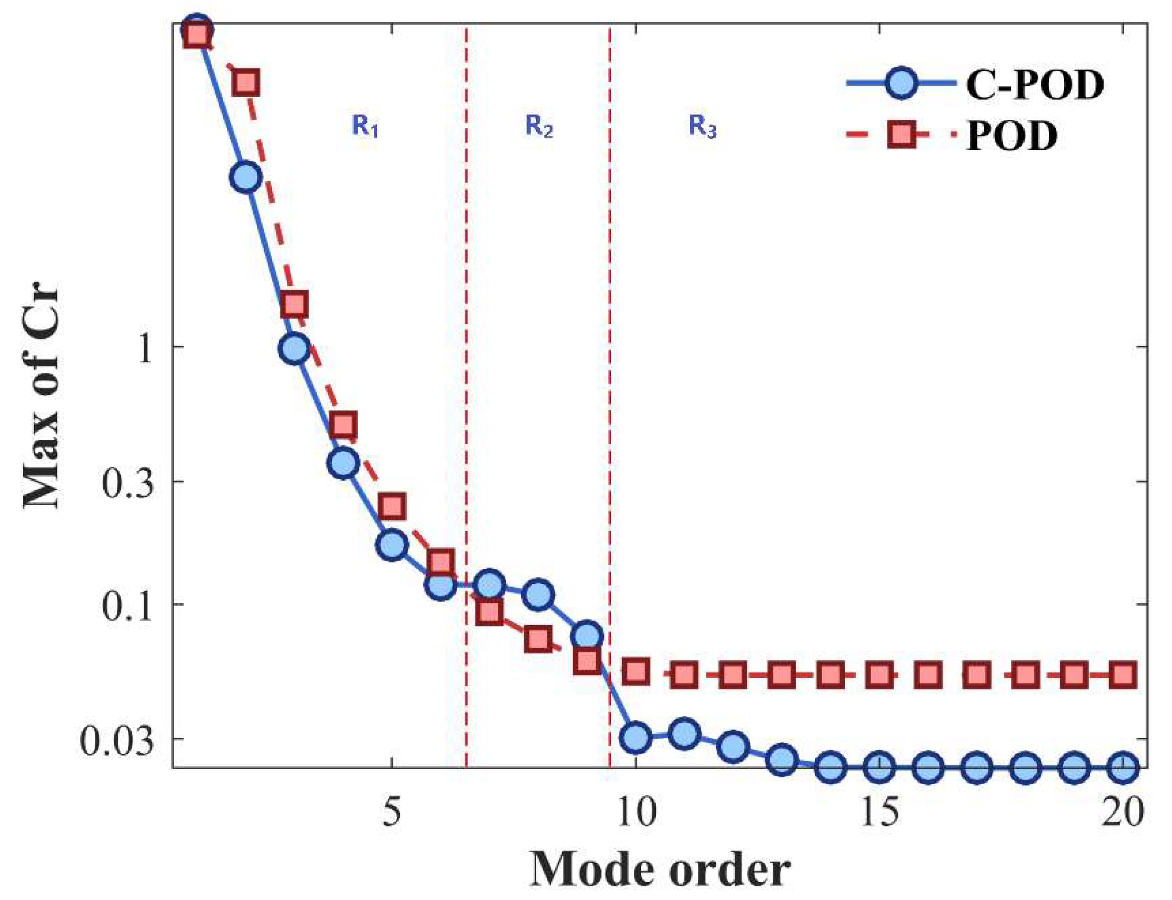
Figure 5.
Evolution of the Burgers' Equation Waveform and the First Mode for c=0.1, β=0.2 and t=0 to t=2.
Figure 5.
Evolution of the Burgers' Equation Waveform and the First Mode for c=0.1, β=0.2 and t=0 to t=2.
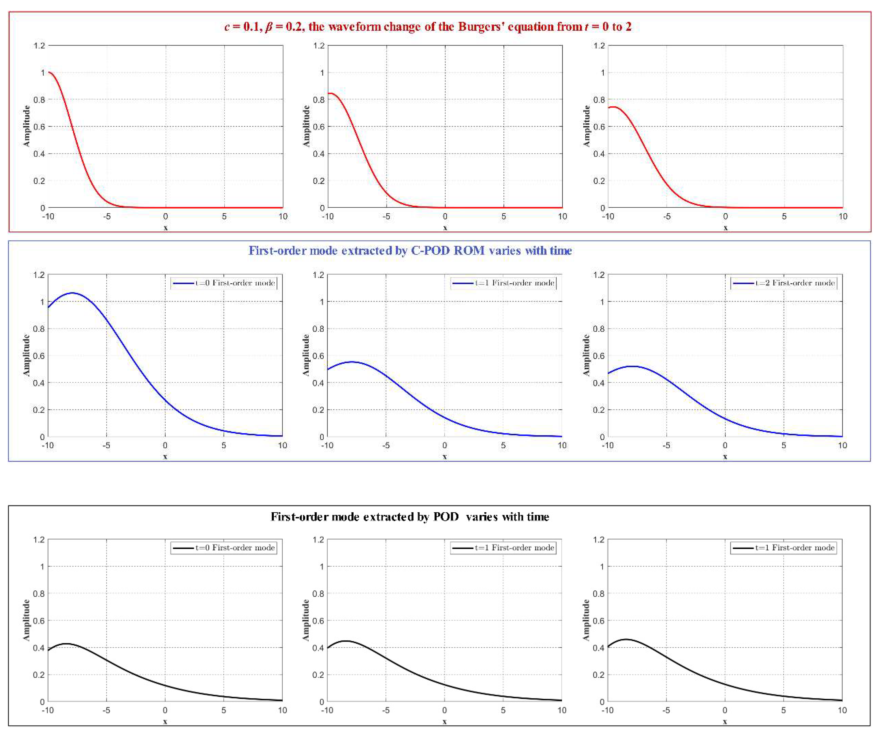
Figure 6.
Evolution of the Burgers' Equation Waveform and the First Mode for c=2, β=2 and t=0 to t=2.
Figure 6.
Evolution of the Burgers' Equation Waveform and the First Mode for c=2, β=2 and t=0 to t=2.
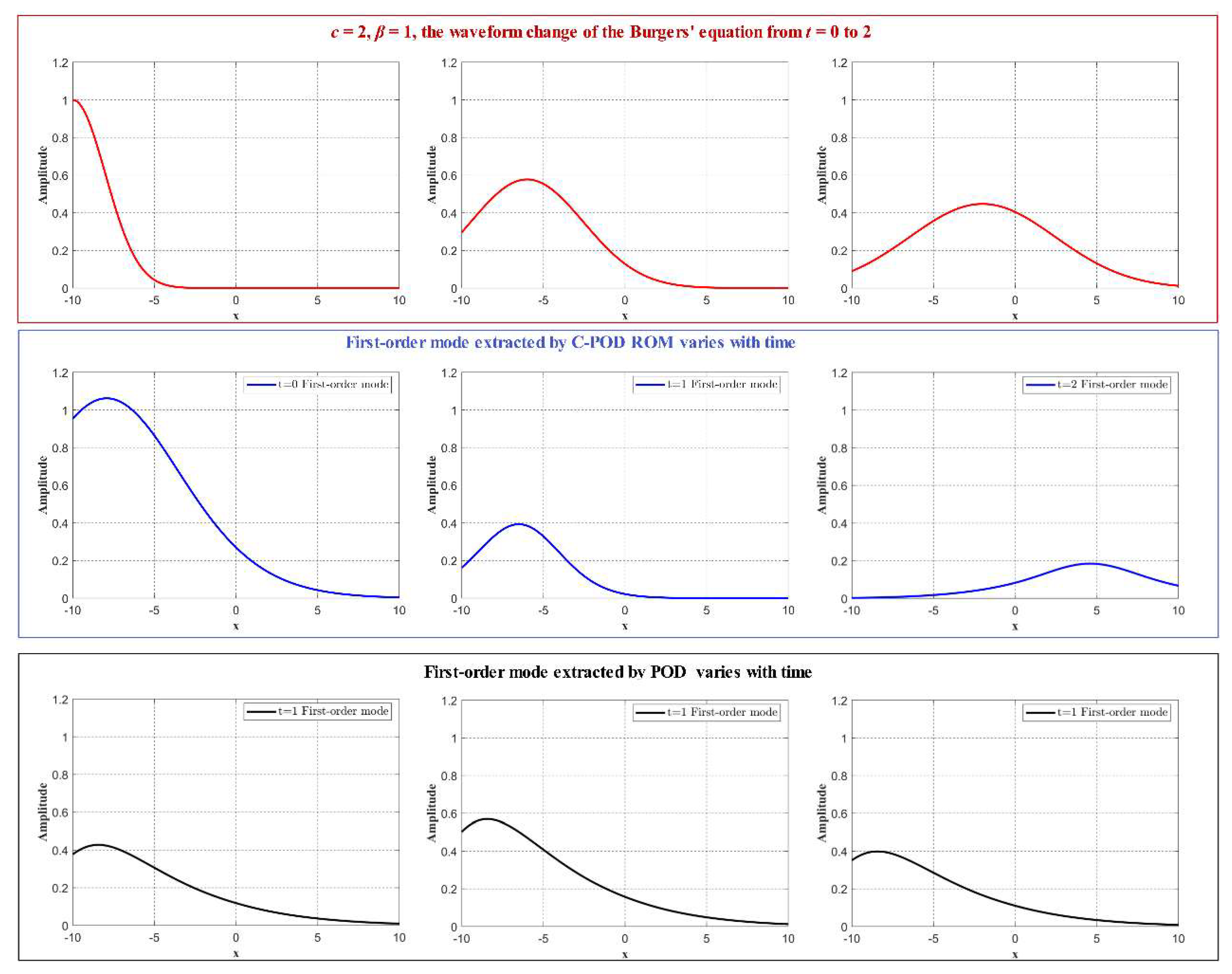
Figure 7.
Geometric dimensions of the computational domain for the two-dimensional cylinder wake flow.
Figure 7.
Geometric dimensions of the computational domain for the two-dimensional cylinder wake flow.
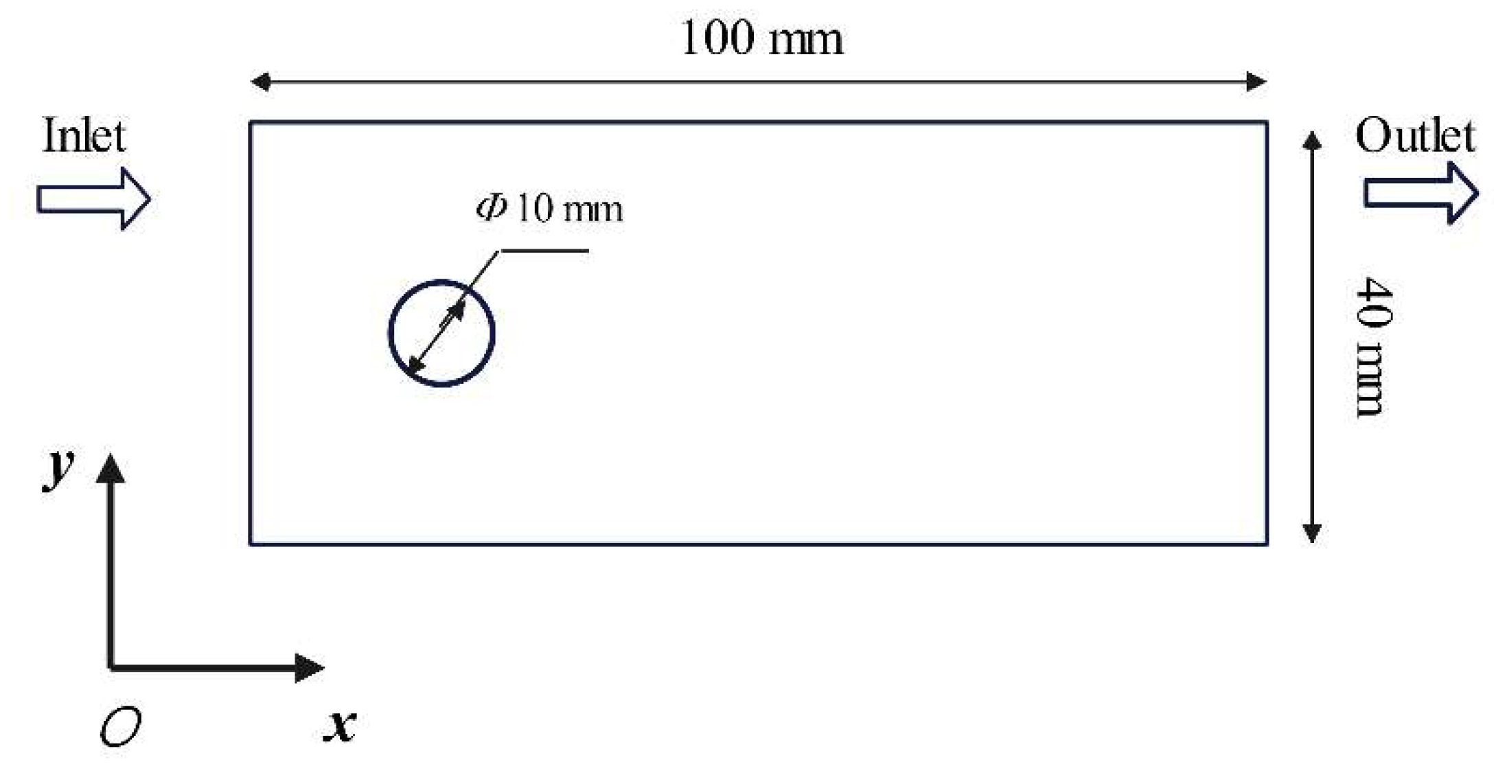
Figure 8.
Typical Flow Patterns in the Wake of a Cylinder at Re=150.
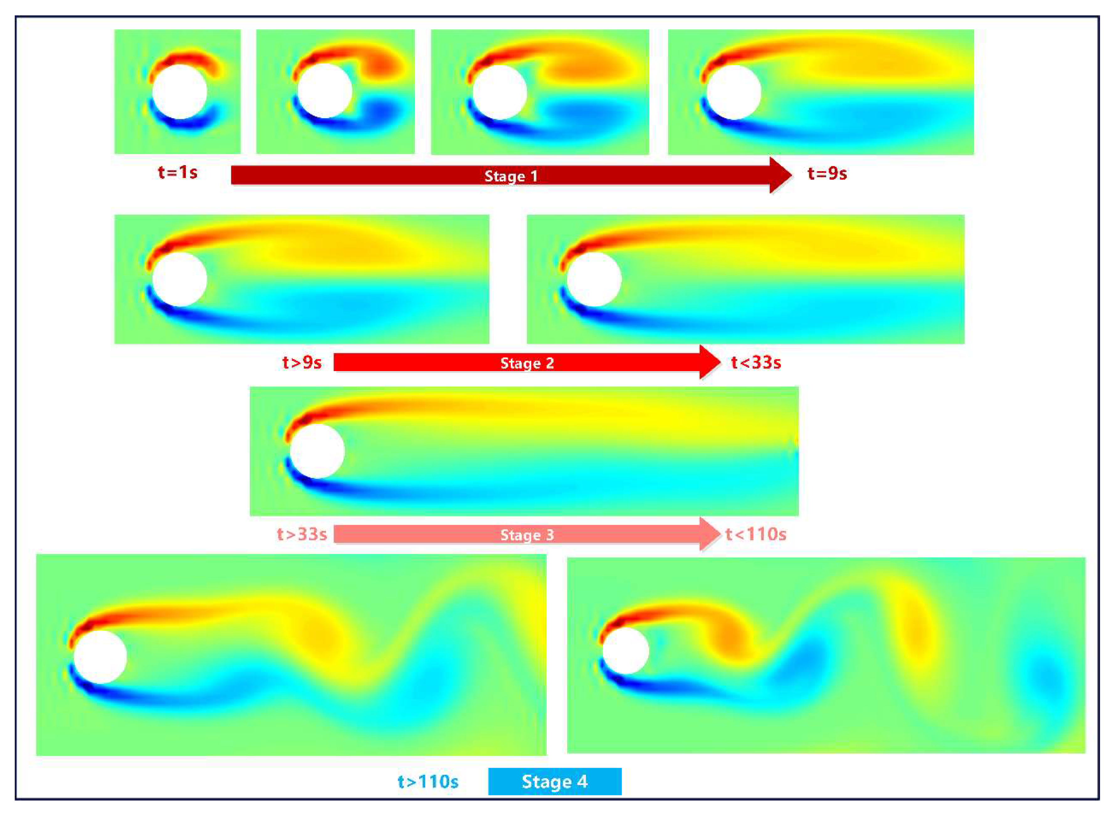
Figure 9.
Variation in Average Dimensionality Reduction and Reconstruction Capability of POD and C-POD Methods at Different Modal Orders.
Figure 9.
Variation in Average Dimensionality Reduction and Reconstruction Capability of POD and C-POD Methods at Different Modal Orders.
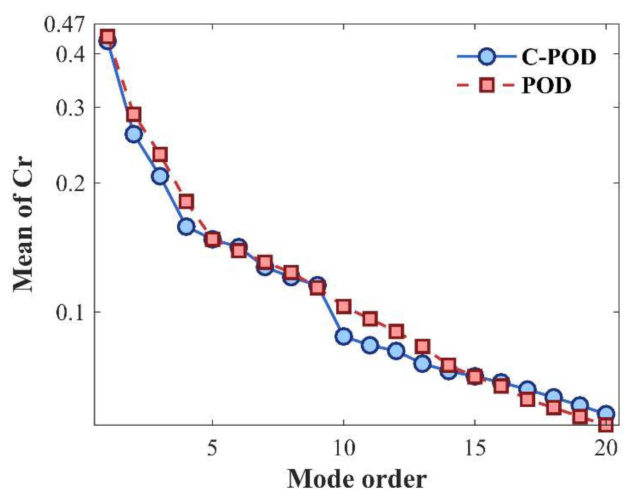
Figure 10.
Variation in the Lower Bound of Dimensionality Reduction and Reconstruction Capability of POD and C-POD Methods at Different Modal Orders.
Figure 10.
Variation in the Lower Bound of Dimensionality Reduction and Reconstruction Capability of POD and C-POD Methods at Different Modal Orders.
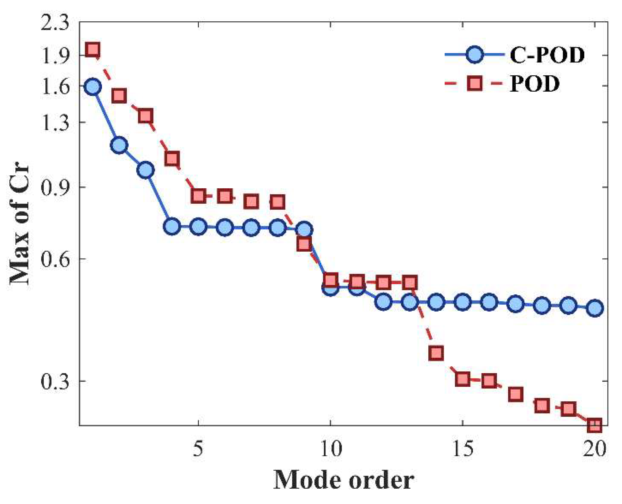
Figure 11.
Distribution of the Vorticity Field Dominated by the First Six Modes Extracted by C-POD and POD at t=236 s.
Figure 11.
Distribution of the Vorticity Field Dominated by the First Six Modes Extracted by C-POD and POD at t=236 s.
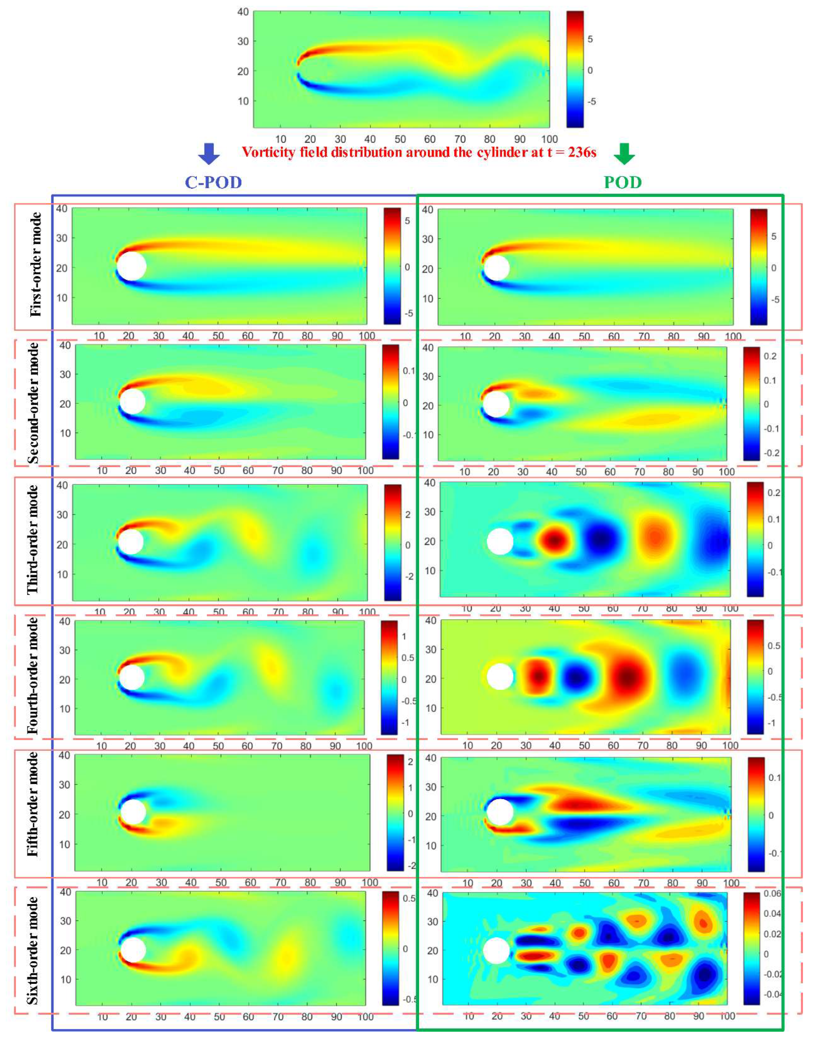
Figure 12.
Distribution of the Vorticity Field Dominated by the First Six Modes Extracted by C-POD and POD at t=240 s.
Figure 12.
Distribution of the Vorticity Field Dominated by the First Six Modes Extracted by C-POD and POD at t=240 s.
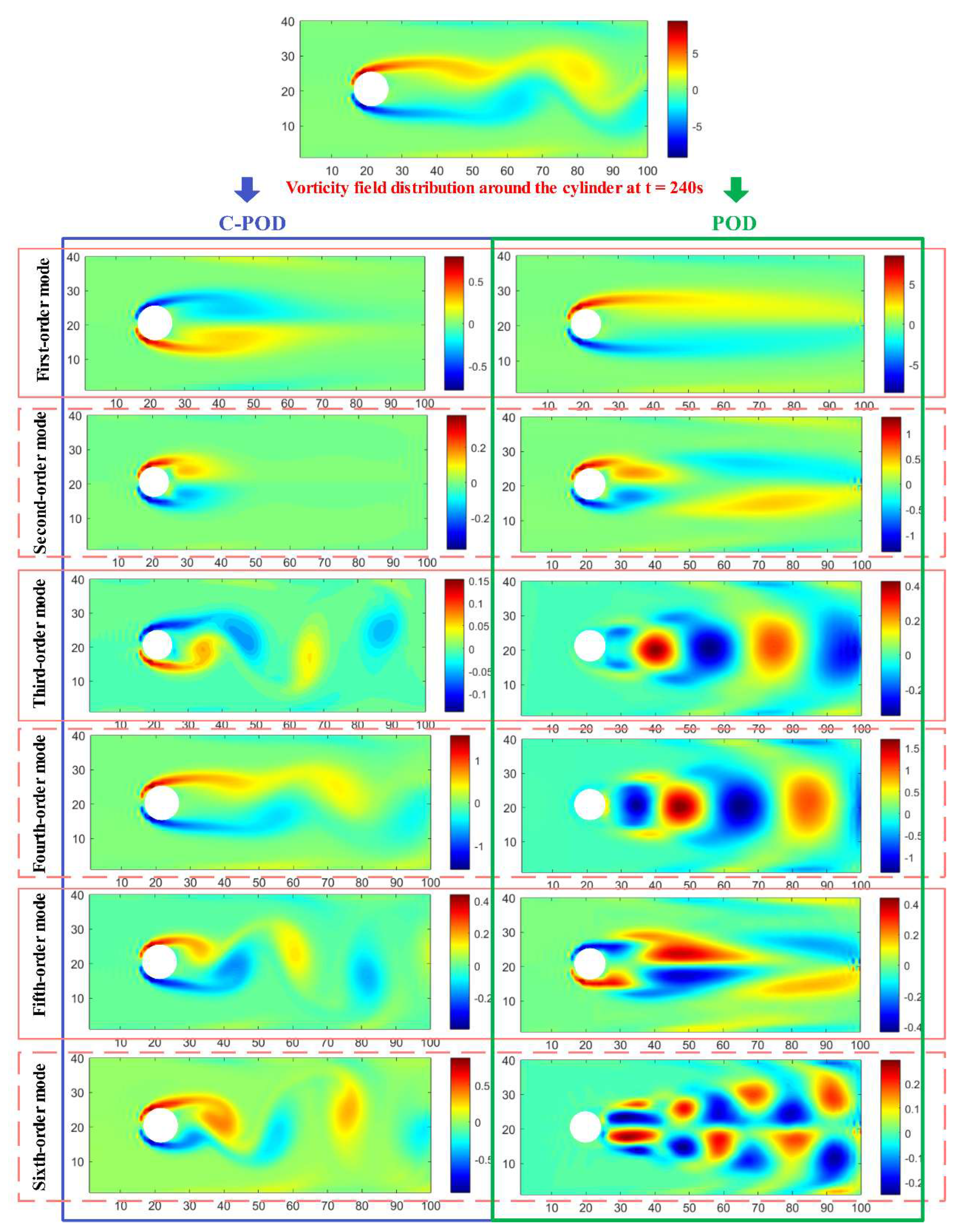
Figure 13.
Various Vortex Patterns in the Vorticity Field Dominated by C-POD ROM Modes.
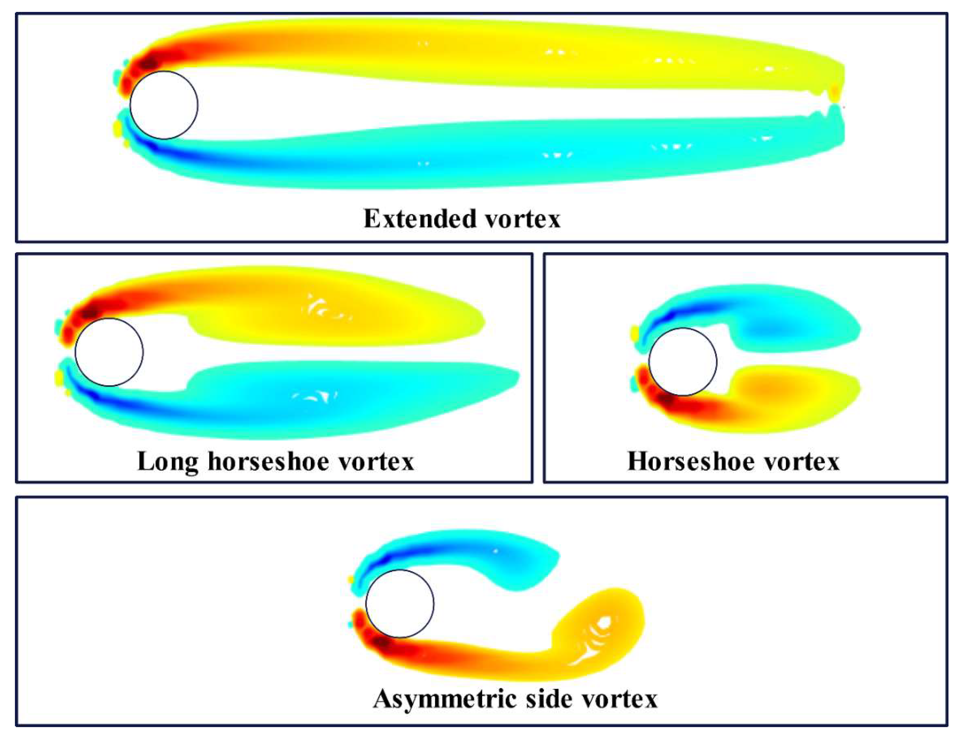
Figure 14.
Comparison of Reconstruction Accuracy for the First n Modes Extracted by POD and C-POD Methods.
Figure 14.
Comparison of Reconstruction Accuracy for the First n Modes Extracted by POD and C-POD Methods.
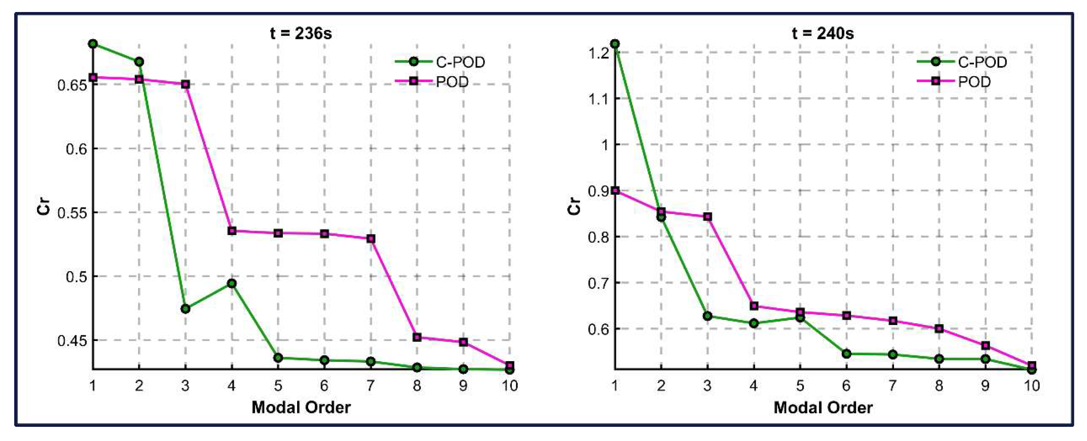
Figure 15.
Temporal Variation of the First and Second Modal Coefficients Extracted by C-POD ROM Using the ECEPM Method.
Figure 15.
Temporal Variation of the First and Second Modal Coefficients Extracted by C-POD ROM Using the ECEPM Method.
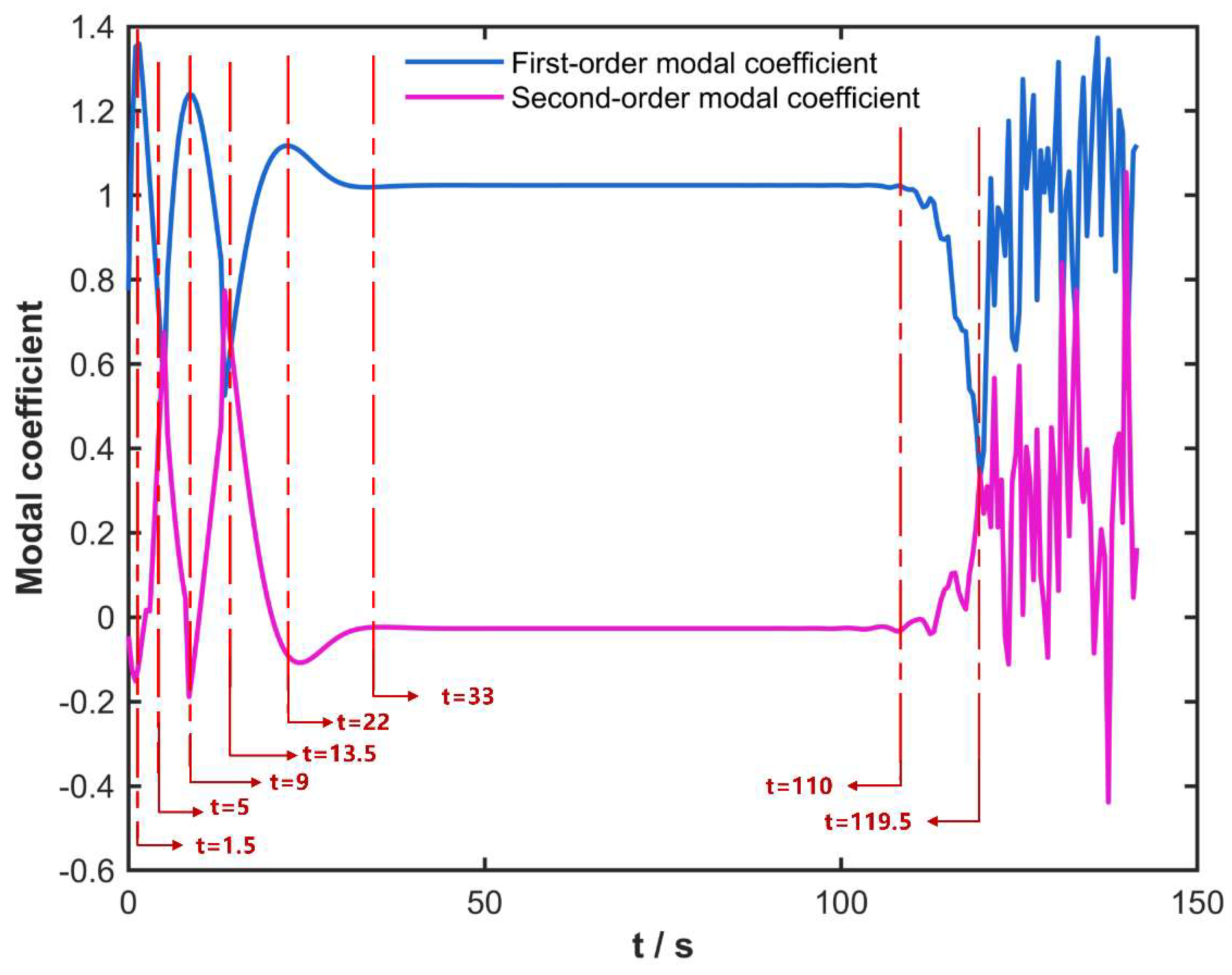
Figure 16.
Temporal Changes in the Vorticity Field Dominated by the First and Second Modes of C-POD ROM at t=1.5, 5, and 9s.
Figure 16.
Temporal Changes in the Vorticity Field Dominated by the First and Second Modes of C-POD ROM at t=1.5, 5, and 9s.
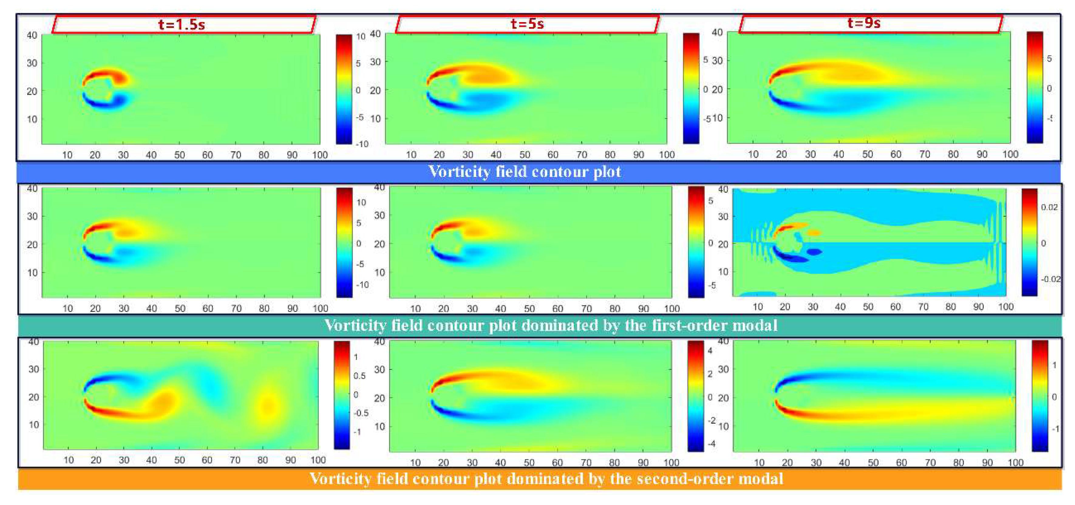
Figure 17.
Temporal Changes in the Vorticity Field Dominated by the First and Second Modes of C-POD ROM at t=13.5, 22, and 33s.
Figure 17.
Temporal Changes in the Vorticity Field Dominated by the First and Second Modes of C-POD ROM at t=13.5, 22, and 33s.
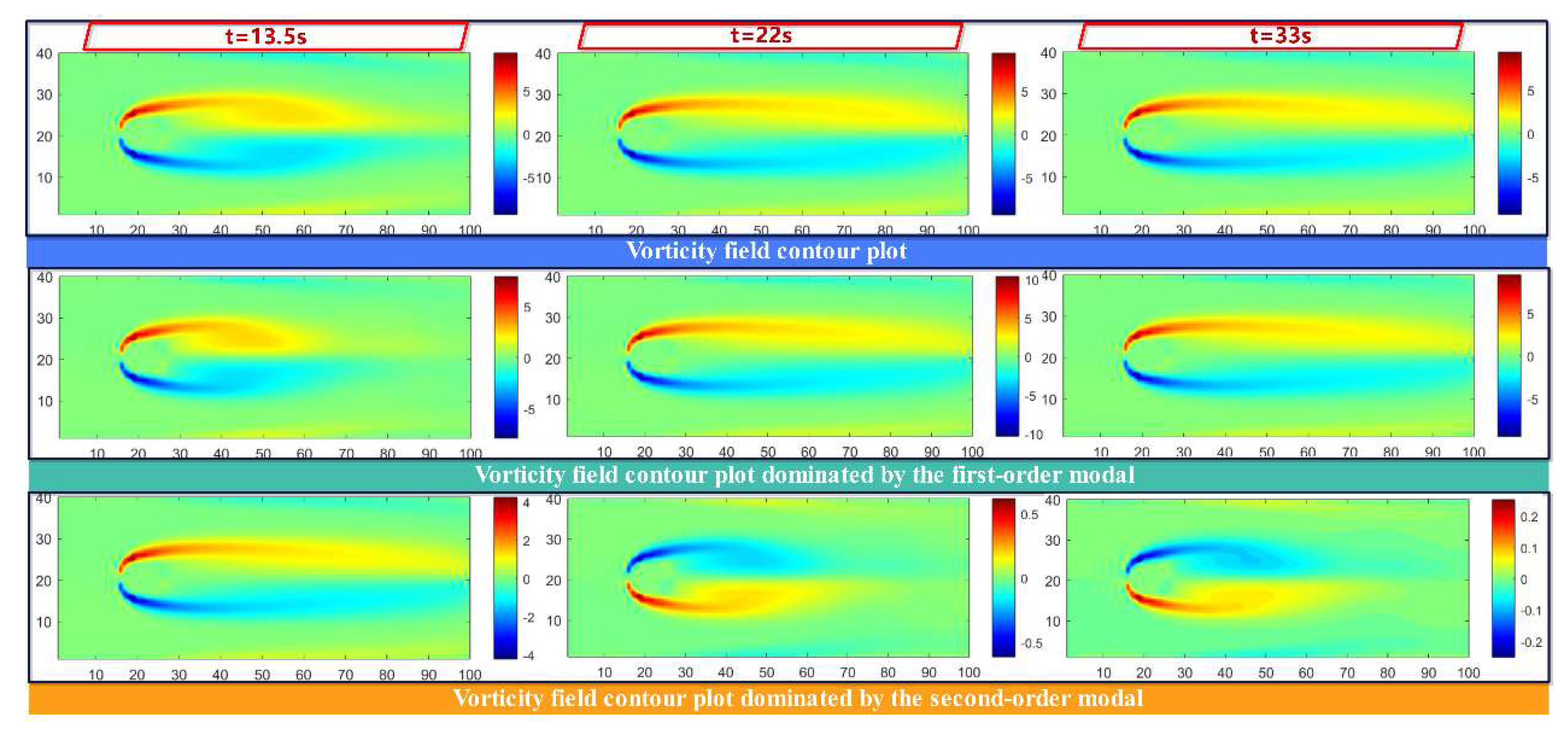
Figure 18.
Temporal Changes in the Vorticity Field Dominated by the First and Second Modes of C-POD ROM at t=110, 119.5, and 135s.
Figure 18.
Temporal Changes in the Vorticity Field Dominated by the First and Second Modes of C-POD ROM at t=110, 119.5, and 135s.
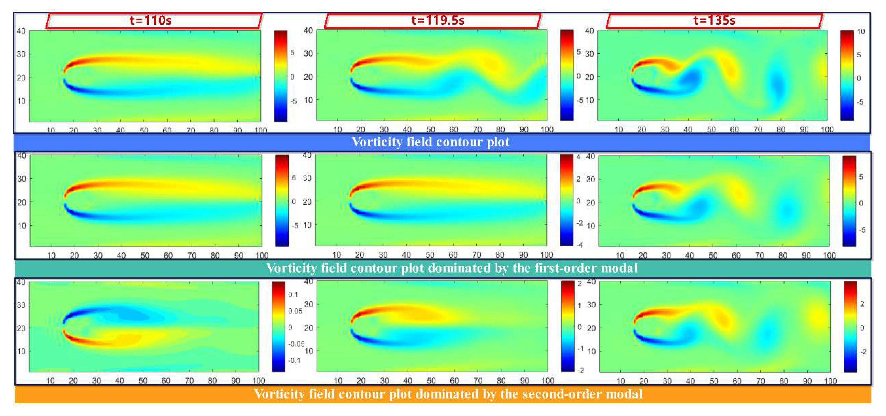
Figure 19.
Variation in the Average Field Reconstruction Capability of Gappy POD and Gappy C-POD Methods at Different Modal Orders.
Figure 19.
Variation in the Average Field Reconstruction Capability of Gappy POD and Gappy C-POD Methods at Different Modal Orders.
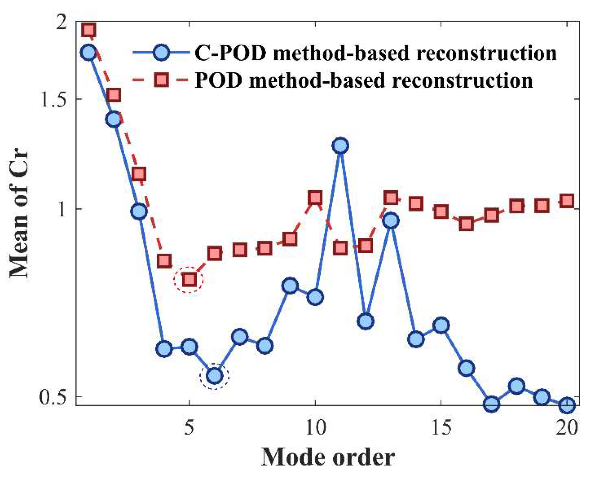
Figure 20.
Variation in the Lower Bound of Field Reconstruction Capability for Gappy POD and Gappy C-POD Methods at Different Modal Orders.
Figure 20.
Variation in the Lower Bound of Field Reconstruction Capability for Gappy POD and Gappy C-POD Methods at Different Modal Orders.

Figure 21.
Gappy POD reconstruction of the cylinder wake vorticity field at t=141s.
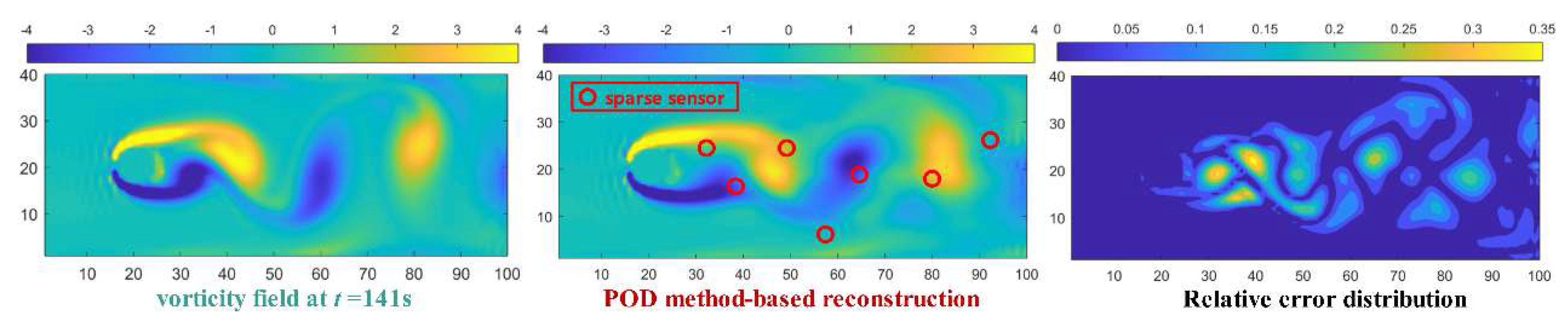
Figure 22.
Gappy C-POD Reconstruction of the Cylinder Wake Vorticity Field at t=141s.
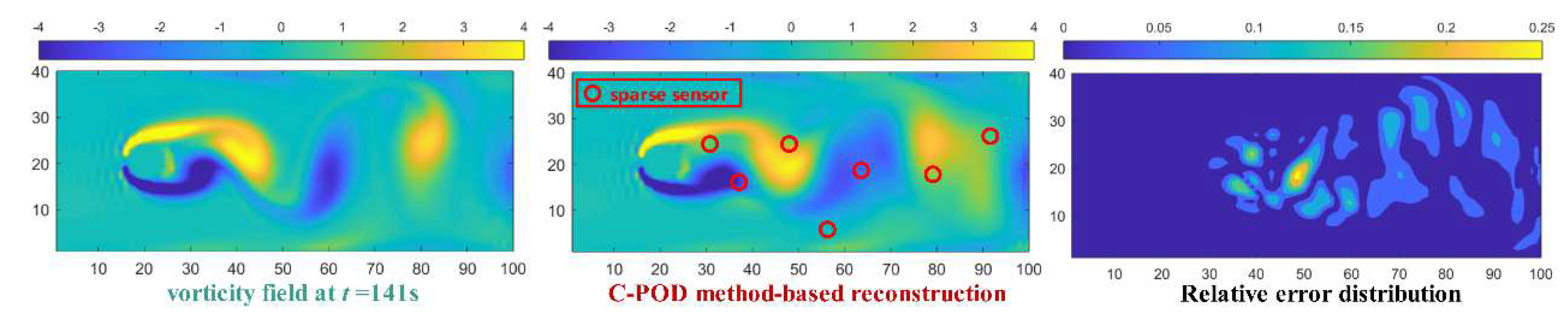

Table 1.
Comparison of Numerical Solutions with Literature Results for Varying Total Grid Numbers and Dimensionless Time Steps.
Table 1.
Comparison of Numerical Solutions with Literature Results for Varying Total Grid Numbers and Dimensionless Time Steps.
| Operating Condition Name | Total Number of Grids | CD | St | |
|---|---|---|---|---|
| A1 | 100◊40 | 0.01 | 0.215 | 0.16 |
| A2 | 200◊80 | 0.01 | 0.225 | 0.164 |
| A3 | 400◊160 | 0.01 | 0.229 | 0.165 |
| A4 | 600◊240 | 0.01 | 0.229 | 0.165 |
| A5 | 800◊320 | 0.01 | 0.229 | 0.165 |
| A6 | 400◊160 | 0.005 | 0.229 | 0.165 |
| A7 | 400◊160 | 0.02 | 0.231 | 0.167 |
| Experiment from [26] | 0.165 | |||
| CFD from [27] | 0.226 | 0.165 | ||
| CFD from [28] | 0.233 | 0.166 |
Disclaimer/Publisher’s Note: The statements, opinions and data contained in all publications are solely those of the individual author(s) and contributor(s) and not of MDPI and/or the editor(s). MDPI and/or the editor(s) disclaim responsibility for any injury to people or property resulting from any ideas, methods, instructions or products referred to in the content. |
© 2025 by the authors. Licensee MDPI, Basel, Switzerland. This article is an open access article distributed under the terms and conditions of the Creative Commons Attribution (CC BY) license (http://creativecommons.org/licenses/by/4.0/).
Copyright: This open access article is published under a Creative Commons CC BY 4.0 license, which permit the free download, distribution, and reuse, provided that the author and preprint are cited in any reuse.


