
Submitted:
28 August 2024
Posted:
29 August 2024
You are already at the latest version
Abstract
A reduced-dimension (RD) method based on the proper orthogonal decomposition (POD) technology and the linearized Crank-Nicolson mixed finite element (CNMFE) scheme for solving the 2D nonlinear Extended Fisher-Kolmogorov (EFK) equation is proposed. The method reduces CPU runtime and error accumulation by reducing the dimension of the unknown CNMFE solution coefficient vectors. For this purpose, The CNMFE scheme of the EFK equation is established and the uniqueness, stability and convergence of the CNMFE solutions are discussed. Subsequently, the matrix-based RDCNMFE scheme is derived by applying the POD method. Furthermore, the uniqueness, stability and error estimates of the linearized RDCNMFE solution are proved. Finally, numerical experiments are carried out to validate the theoretical findings. In addition, we contrast the RDCNMFE method with the CNMFE method, highlighting the advantages of the dimensionality reduction method.
Keywords:
extended fisher-kolmogorov equation
; proper orthogonal decomposition
; mixed finite element
; uniqueness and stability
; error estimates
; numerical experiment
1. Introduction
The primary goal of this research is to apply the POD-based reduced-dimension method to solve the following 2D nonlinear extended Fisher-Kolmogorov (EFK) equation
in which is a bounded convex polygonal domain with boundary . is the time interval, where . Coefficient is a positive constant. is known initial function. , is the Lipschitz continuous function of u, that is, there exists a positive constant C such that
For simplicity, we assume that in the following theoretical analysis.
When in (1), the second-order diffusion equation is obtained, which is called the standard Fisher-Kolmogorov equation. Coullet et al. [2] added a stabilizing fourth-order derivative term to obtain the equation (1), and called it as the extended Fisher-Kolmogorov equation. The EFK equation has very important physical background. It was applied to various kinds of physics and engineering. Because of the complexity of the equation, it is difficult to get its analytical solution. Therefore, it is very important to solve the equation numerically. And there have been a lot of research results on this equation. For instance, direct local boundary integral equation method [3], Fourier pseudo-spectral method [4], and modified cubic B-spline and polynomial based differential quadrature method [5,6] are applied to solve the EFK equation. Various four-order finite difference schemes [7,8,9,10] have been developed to solve the EFK equations, which have the four-order and second-order accuracy in space and time variables, respectively. He [11] used a three-level linearly implicit finite difference method to solve the 1D and 2D EFK equation, and the method is second-order convergent both in time and space direction. Sweilam et al. [12] studied stochastic EFK equation by combining the compact finite difference scheme and the semi-implicit Euler-Maruyama approach. Danumjaya and Pani [13] applied mixed finite element methods to solve the EFK equation with different types of boundary conditions. Doss and Nandini [14] employed a splitting technique to derive an H-Galerkin mixed finite element scheme for the EFK equation. Wang et al. [15] used a new linearized CNMFE method to study the EFK equation, in which belongs to the weaker space instead of the classical space. In this paper, we establish the CNMFE scheme for the 2D EFK equation and analysis the uniqueness, stability and convergence of the CNMFE solutions.
However, in practical problems, using CNMFE method to solve EFK equations is a problem with a large number of unknowns, which makes running extremely slow, leads to an increase in rounding errors, and makes it difficult to obtain accurate numerical solutions. Therefore, it is crucial to lessen the number of unknowns in the CNMFE method of EFK equation to reduce the computational load, save CPU running time, and minimize the accumulation of rounding errors in the calculation process. The Proper orthogonal decomposition (POD) technology, reducing the amount of unknowns in numerical schemes, is an efficient dimensionality reduction method for solving partial differential equations (PDEs). It reduces the CPU running time and reduces the accumulation of round-off errors. POD technology can be applied to numerical methods of various PDEs, such as finite difference method [16,17,18], Schwarz domain decomposition method [19], finite spectral element method [20,21] etc. For reduced dimension FE and MFE models based on POD techniques, there are two dimensionality reduction method. One method is that the optimized models are established through reducing the dimension of the FE or MFE subspace. The parabolic equation [22], Sobolev equation [23], Burgers equation [24] and some other PDEs [25,26,27,28] are solved by the reduced-dimension method of constructing the POD subspace. The other is a new reduced-dimension method for the CNFE [29,30] and CNMFE [31,32,33,34] solution coefficient vectors proposed by Luo et al. in 2020. In [35], Luo and Yang combined unknown solution coefficient vector dimensionality reduction method and continuous space-time finite element method to study the 2D non-stationary incompressible Navier-Stokes equations.
Although there are existing reduce-order methods of the EFK equation, such as Literature [17], which combines the high-order compact finite difference scheme with the POD method to obtain the spatial sixth-order accuracy while greatly shortening the calculation time. Literature [33] uses the POD technique to reduce the dimensionality of the two-grid CNMFE solution coefficient vectors, in which, the matrix theory is used to deeply explore the stability and convergence of the TGRDECNMFE solutions. However, the reduce-dimension method proposed in this paper is theoretically significantly different from the above research methods. This paper integrates POD technology with the linearized CNMFE method, and proposes a new reduce-dimension method for 2D nonlinear EFK equations. In this study, we adopt the CN fully discrete format in the temporal direction to achieve second-order time accuracy. Additionally, we linearize the nonlinear term to significantly enhance computational speed and efficiency while preserving model accuracy. Unlike Literature [33], our work utilizes traditional finite element techniques to analyze uniqueness, stability, and convergence of the RDCNMFE solutions. Our proposed method combines the advantages of POD and linearized CNMFE methods for effective dimensionality reduction of the nonlinear EFK equation. This approach not only maintains accuracy but also greatly improves computational speed and efficiency, providing a novel insight and solution for solving the EFK equation.
The structure of this paper is as follows. In Section 2, we propose the CNMFE scheme and discuss the uniqueness, stability and convergence of the CNMFE solutions. In Section 3, we generate the POD basis to derive the reduce-dimension matrix model of the CNMFE solution coefficient vectors and analysis the uniqueness, stability and error estimate of the RDCNMFE solutions. In Section 4, we employ the numerical experiment of the 2D EFK equation to verify the effectiveness of RDCNMFE method and correctness of theoretical analysis. In Section 5, we summarize the major conclusions and findings.
2. The Crank-Nicolson Mixed Finite Element Method of the EFK Equation
2.1. The CNMFE Schemes
The Sobolev spaces and their corresponding norms mentioned in this paper adhere to standard definitions (see [1]). In order to develop the CNMFE scheme of the EFK equation (1), we initially introduce a diffusion term , resulting in the following two lower-order equations
Let . With the Green’s formula, the mixed functional form of (3) is as follows.
Problem 1.
Find : satisfying
Let be the quasi-uniform triangulation subdivision on . The FE subspace , spanned by the orthonormal basis under the inner product in , is defined as follows:
in which is generated by th degree polynomials on .
For given integer , let , , and . Therefore, we can rewrite Problem 1 at time in the following form.
Then, the equivalent expression of (6) is as follows.
where
Let represent the CNMFE approximations of solutions for Problem 1 at . Thus, the CNMFE model of Problem 1 can be constructed as follows.
Problem 2.
Find satisfying
Remark 1.
By means of a linearized term
we can observe that the formulation (11) is a linear scheme.
2.2. The Uniqueness, Stability and Convergence of the CNMFE Solutions
By employing the base functions of the FE space , the solutions of Problem 2 can be formulated in the form of
where is the orthonormal base, satisfied
and are the unknown coefficient vectors of CNMFE solutions. From the expression of the solutions of (13), Problem 2 can be represented equivalently in the following matrix model.
Problem 3.
Find and satisfying
where
and
Theorem 1.
The Problem 3 has the unique solutions .
Proof of Theorem 1.
Problem 3 can be written as
where stands for the unit matrix, and denotes zero column vector of .
From the definitions of matrices and , we know that they are positive definite and thus invertible. From (15), we can conclude that the coefficient matrix is invertible as well. Hence, there exists a unique set of solutions for Problem 3.
□
In order to prove the stability of the CNMFE solutions, we need to introduce the properties of in Problem 3.
Lemma 1.
[[36], Lemma 1.19] Matrix satisfies the following inequality
Theorem 2.
Both the CNMFE solutions and their solution coefficient vectors are unconditionally stable.
Proof of Theorem 2.
We represent (14) as
Substituting the second formula of (17) into the first formula, we obtain
Taking the inner product of (18) and , we have
The left side of (19) is that
and the right side of (19) is that
Combining lemma 1 with the global Lipschitz-continuity of , the first term of (21) can be estimated as
where and are bounded. Combining (20), (21) and (22) we have
Multiplying both sides of the inequality of (23) by and summating from 2 to , we have
noting that , then
Applying the Gronwall Lemma to (25), we obtain
And because
From (26) and (27), we have
Due to , we can easily get
(28) and (29) indicate that the CNMFE solutions and their coefficient vectors are unconditionally stable.
□
In order to analyze the convergence of the linearized CNMFE scheme, we first need to establish the projection operator .
Lemma 2.
Let satisfy the following relation
and
In order to facilitate theoretical analysis, the errors can be decomposed into
Subtracting (11) from (7) and using (30) at , we obtain the following error equations.
In order to obtain the error estimates, we introduce the following lemma, which is easily obtained by Taylor expansion.
Lemma 3.
and satisfy the following estimates
Based on Lemmas 2 and 3, the following theorems for Crank-Nicolson fully discrete error estimates is obtained.
Theorem 3.
With , assume that the solution’s regular properties for (4) satisfy , , . Then there exists a positive constant C independent of h and such that
where .
Proof of Theorem 3.
Taking and in (35) and (36), respectively, we obtain
Multiplying (41) by and adding it to (40) and using Cauchy-Schwarz inequality and Young inequality, we obtain
For the nonlinear term , Using Young inequality, we have
Noting that
Substitute (43) and (44) into (42) to obtain
Summing from , the resulting inequality becomes
Choosing , when , , and using discrete Gronwall Lemma and Lemma 3, we obtain
Combining Lemma 2, (47) and the triangle inequality, the proof of (39) is accomplished.
□
Theorem 4.
With and ,assume that the solution’s regular properties for (4) satisfy , , . Then there exists a positive constant C independent of h and such that
where .
Proof of Theorem 4.
From (36) we can get
Taking and in (35) and (49), respectively, we obtain
Multiplying (51) by and adding it to (50) and using Cauchy-Schwarz inequality and Young inequality, we have
Similar to (44),
Multiplying (52) by , summing from and using (43), (44) and (53) to obtain
Using the Gronwall Lemma, we have
Substitute (47) and Lemma 3 into (55), we get
Combining Lemma 2, (56) with the triangle inequality, we complete the proof. □
3. The reduced-dimension method of the Crank-Nicolson mixed finite element solution coefficient vectors of the EFK equation
3.1. Construction of POD basis vectors
Firstly, we need to compute the initial K-step solution coefficient vectors of Problem 3, which will yield two snapshot matrices and . Secondly, we need to compute the positive eigenvalues and arrange them in descending order of , and the associated eigenvectors to form the matrix . Finally, choosing the first d column vectors of as a set of POD bases , they satisfy the following equalities
where and of vector . When , it follows that
Here, denotes the unit vectors whose nth component is 1. Therefore, is a set of optimal POD bases.
Remark 2.
Since the order of matrix is much larger than the order of matrix , and the eigenvalues of and are equal, thus we first calculate the initial d eigenvalues of matrix and their corresponding eigenvectors . Then we use the relation to obtain the eigenvectors of , and generate a set of POD basis vectors .
3.2. Formulation of the RDCNMFE scheme
Firstly, letting , , and and represent the RDCNMFE solution coefficient vectors. Secondly, we can instantly obtain the first K RDCNMFE solution vectors and from section 3.1. Finally, by using instead of in Problem 3, the following matrix-based RDCNMFE scheme can be established.
Problem 4.
Find and satisfying
in which are the first K solution coefficient vectors for Problem 3. The definitions of matrix , vector , as well as FE basis function vectors are given in section 2.2.
3.3. The uniqueness, stability and error estimate of the RDCNMFE solutions
For the RDCNMFE solutions of Problem 4, the unique, stable and convergent properties are as follows.
Theorem 5.
Under the same assumptions as Theorem 3 and 4, if are the weak solutions to Problem 1 and are the solutions to Problem 4, then for any , the RDCNMFE solutions have uniqueness and unconditional stability, and the following error estimate is obtained.
Proof of Theorem 5.
(1) Discuss the uniqueness of the RDCNMFE solutions.
-
For , Theorem 1 guarantees the uniqueness of solutions to problem 3. Therefore, the solutions generated from first and fourth formulas in problem 4 must also be unique.For , using , , the last three formulas of Problem 4 can be converted toFor , the set of solutions for Problem 3 is unique. Since (62) – (64) follow the same formats as problem 3, the set of solutions for (62) – (64) is also unique.
- (2)
-
Demonstrate the stability of the RDCNMFE solutions.When , since the vectors in and are orthonormal, using Theorem 2, we haveWhen , since is a positive definite symmetric matrix, we can rewrite (62) asPutting (63) into (66), we haveTaking the inner product of (67) and ,Then the left side of (68) is thatand the right side of (68) is thatUsing the same technique as (22), we haveCombining (69), (70) and (71), we haveMultiplying both sides of (72) by , and summating from 2 to n, we obtainNoting thatputting (74) into (73), we haveUsing the Gronwall Lemma for (75),AndSo we haveThus, noting that , we getFrom (65) and (79), the RDCNMFE solutions are unconditional stable.
- (3)
-
Analyse the error estimate of the RDCNMFE solutions.When , from , (58) and (59), we haveWhen , letting and , and combining (17), (66) and (63), we obtainPutting (82) into(81), we haveTaking the inner product of (83) and ,Then the left side of (84) is thatand the right side of (84) is thatCombining Lemma 1 with the global Lipschitz-continuity of , the first term of (86) can be estimated asCombining (85), (86) and (87), we haveMultiplying both sides of (88) by , and summating from to , we obtainNoting thatPutting (90) into (89), from (58) and (59), we haveApplying the Gronwall Lemma for (91),Andthus, we getFurther, from , we obtainUsing the triangle inequality, Theorem 3 and 4, (80) and (95), we obtain
□
4. The Numerical Examples for the EFK Equations
In order to verify the effectiveness of the RDCNMFE method, we can compare the errors and orders between the genuine, CNMFE and RDCNMFE solutions and CPU runtime on different time nodes. We here adopt the numerical experiment that the following 2D nonlinear EFK equation has a genuine solution. Generally speaking, it has no genuine solution.
in which , we may obtain the genuine solution of (97). The genuine solution of the auxiliary variable is .
Firstly, the initial 20 CNMFE solution vectors are obtained by calculating Problem 3 to establish the snapshot matrixes and . Secondly, we calculate the eigenvalues (arranged decreasingly) and the associated eigenvectors of the matrixes . Then, we find that , so that we just need to extract the first 6 eigenvectors of the matrix to construct a set of POD basis vectors , where . Finally, we compute the RDCNMFE solutions of (97) by Problem 4 and the CNMFE solutions of (97) by Problem 3 when and at . And they are compared with the genuine solution respectively, exhibited in Figure 1 and Figure 2. As evident from Figure 1 and Figure 2, the RDCNMFE and CNMFE solutions closely mirror the genuine solution.
For comparison, we give the errors and convergence orders of the CNMFE and RDCNMFE solutions for u and at in Table 1 and Table 2, respectively. As can be observed from Table 1 and Table 2, the errors and convergence rates of the RDCNMFE method are nearly identical to the CNMFE method, which aligns with the previous theoretical analysis. Figure 3 offers a more visual representation of the comparative results of the error convergence orders between and and between and .
To provide additional evidence for the effectiveness of the RDCNMFE method, we recorded the errors and the CPU running time for computing the CNMFE and RDCNMFE solutions at , respectively. These results are obtained by solving Problems 3 and 4 and shown in Table 3.
As demonstrated in Table 3, with the increase of time, the CNMFE method with degrees of freedom requires considerable CPU runtime at each time node, where the running time increases by approximately for every additional . While performing at the same time node, the RDCNMFE method, with only degrees of freedom, requires very minimal CPU runtime, with an increase in running time of only about for every additional . The calculation time of the CNMFE method is approximately 70 times greater than that of the RDCNMFE method when . This experiment demonstrates that the RDCNMFE method significantly reduces CPU running time. Furthermore, the results from the Table 3 indicate that the RDCNMFE method produces slightly less errors compared to the CNMFE method. In summary, it is clear that the RDCNMFE method surpasses the CNMFE method, proving it as an effective numerical method for solving the 2D nonlinear EFK equation.
5. Conclusions
In this study, we have focused on the reduced-dimension method of Crank-Nicolson mixed finite element solution coefficient vectors for 2D nonlinear EFK equations In order to give a full demonstration of the effectiveness of the reduced-dimension method, we have established the CNMFE scheme of the 2D nonlinear EFK equation and discussed the uniqueness, stability, and convergence of CNMFE solution. Then, we have generated the POD basis based on the initial K CNMFE solutions, constructed the RDCNMFE matrix model, and employed the traditional finite element techniques to analyze the uniqueness, stability and error estimation of RDCNMFE solution. Additionally, numerical experiments have been conducted to comparatively evaluate the performance of the two methods. Compared with the CNMFE method, the RDCNMFE method has fewer degrees of freedom at each time node. This characteristic enables the RDCNMFE method to greatly reduce computational load, running time, and error accumulation. In particular, this paper has simplified the actual calculation by linearizing the nonlinear term without iterative numerical calculation. Therefore, the RDCNMFE method constitutes a novel numerical technique for tackling nonlinear PDEs.
In future research, we intend to extend the scope of application of this method to PDEs with variable coefficients (in this paper, the coefficient is a constant). Additionally, we believe this approach can be adapted to more complex engineering problems.
Author Contributions
Conceptualization, X.C. and H.L.; methodology, X.C.; numerical simulation, X.C.; formal analysis, X.C.; writing—original draft preparation, X.C.; validation, X.C. and H.L.; writing—review, H.L.; supervision, H.L. All authors have read and agreed to the published version of the manuscript.
Funding
This research was funded by the National Natural Science Foundation of China (12161063) and the Program for Innovative Research Team in Universities of Inner Mongolia Autonomous Region (NMGIRT2207).
Data Availability Statement
No new data were created or analyzed in this study. Data sharing is not applicable to this article.
Acknowledgments
The authors would like to thank the reviewers and editors for their invaluable comments, which greatly refined the content of this article.
Conflicts of Interest
The authors declare no conflicts of interest.
Abbreviations
The following abbreviations are used in this manuscript:
| POD | proper orthogonal decomposition |
| CNMFE | Crank-Nicolson mixed finite element |
| RDCNMFE | reduced-dimension Crank-Nicolson mixed finite element |
| EFK | extended Fisher-Kolmogorov |
References
- Adams, R.A. Sobolev Spaces; Academic Press: New York, USA, 1975. [Google Scholar]
- Coullet, P.; Elphick, C.; Repaux, D. Nature of spatial chaos. Phys. Rev. Lett. 1987, 58, 431–434. [Google Scholar] [CrossRef] [PubMed]
- Ilati, M.; Dehghan, M. Direct local boundary integral equation method for numerical solution of extended Fisher-Kolmogorov equation. Eng. Comput-Germany. 2018, 34, 203–213. [Google Scholar] [CrossRef]
- Liu,F.N.; Zhao, X.P.; Liu, B. Fourier pseudo-spectral method for the extended Fisher-Kolmogorov equation in two dimensions. Adv. Differ. Equ-Ny. 2017, 2017, 1–17.
- Bashan, A.; Ucar, Y.; Yagmurlu, N.M.; Esen, A. Numerical solutions for the fourth order extended Fisher-Kolmogorov equation with high accuracy by differential quadrature method. Sigma. J. Eng. Nat. Sci. 2018, 9, 273–284. [Google Scholar]
- Awasthi, A. Polynomial based differential quadrature methods for the numerical solution of fisher and extended Fisher-Kolmogorov equations. Int. J. Appl. Comput. Math. 2017, 3, 665–677. [Google Scholar]
- Li, S.G.; Xu, D.; Zhang, J.; Sun, C.J. A new three-level fourth-order compact finite difference scheme for the extended Fisher-Kolmogorov equation. Appl. Numer. Math. 2022, 178, 41–51. [Google Scholar] [CrossRef]
- Qiao, L.; Nikan, O.; Avazzadeh, Z. Some efficient numerical schemes for approximating the nonlinear two-space dimensional extended Fisher-Kolmogorov equation. Appl. Numer. Math. 2023, 185, 466–482. [Google Scholar] [CrossRef]
- Kadri, T.; Omrani, K. A fourth-order accurate finite difference scheme for the extended-Fisher-Kolmogorov equation. Bull. Korean Math. Soc. 2018, 55, 297–310. [Google Scholar]
- Ismail, K.; Atouani, N.; Omrani, K. A three-level linearized high-order accuracy difference scheme for the extended Fisher-Kolmogorov equation. Eng. Comput-Germany. 2021, 2, 1–11. [Google Scholar] [CrossRef]
- He, D.D. On the L∞-norm convergence of a three-level linearly implicit finite difference method for the extended Fisher-Kolmogorov equation in both 1D and 2D, Comput. Math. Appl., 2016, 71, 2594–2607. [Google Scholar] [CrossRef]
- Sweilam, N.H.; Elsakout, D.M.; Muttardi, M.M. Numerical solution for stochastic extended Fisher-Kolmogorov equation. Chaos, Solitons and Fractals. 2021, 151, 111213.
- Danumjaya, P.; Pani, A.K. Mixed finite element methods for a fourth order reaction diffusion equation. Numer. Meth. Part. D. E. 2012, 28, 1227–1251. [Google Scholar] [CrossRef]
- Doss, L.J.T.; Nandini, A.P. An H1-Galerkin mixed finite element method for the extended Fisher-Kolmogorov equation. Int. J. Numer. Anal. Model. Ser. B. 2012, 3, 460–485. [Google Scholar]
- Wang, J.F.; Li, H.; He, S.; Gao, W.; Liu, Y. A new linearized Crank-Nicolson mixed element scheme for the extended Fisher-Kolmogorov equation. The Scientific World Journal. 2013, 2013. [Google Scholar] [CrossRef] [PubMed]
- Xu, B.Z.; Zhang, X.H. A reduced fourth-order compact difference scheme based on a proper orthogonal decomposition technique for parabolic equations. Bound. Value. Probl. 2019, 130. [Google Scholar] [CrossRef]
- Xu, B.Z.; Zhang, X.H.; Ji, D.B. A reduced high-order compact finite difference scheme based on POD technique for the two dimensional extended Fisher-Kolmogorov equation. IAENG Int. J. Appl. Math. 2020, 50. [Google Scholar]
- Luo, Z.D.; Teng, F. A reduced-order extrapolated finite difference iterative scheme based on POD method for 2D Sobolev equation. Appl. Math. Comput. 2018, 329, 374–383. [Google Scholar] [CrossRef]
- Song, J.P.; Rui, H.X. A reduced-order Schwarz domain decomposition method based on POD for the convection-diffusion equation. Comput. Math. Appl. 2024, 160, 60–69. [Google Scholar] [CrossRef]
- Luo, Z.D.; Teng, F.; Xia, H. A reduced-order extrapolated Crank-Nicolson finite spectral element method based on POD for the 2D non-stationary Boussinesq equations. J. Math. Anal. Appl. 2019, 471, 564–583. [Google Scholar] [CrossRef]
- Luo, Z.D.; Jiang, W.R. A reduced-order extrapolated Crank-Nicolson finite spectral element method for the 2D non-stationary Navier-Stokes equations about vorticity-stream functions. Appl. Numer. Math. 2020, 147, 161–173. [Google Scholar] [CrossRef]
- Luo, Z.D.; Li, L.; Sun, P. A reduced-order MFE formulation based on POD method for parabolic equations. Acta. Math. Sci. 2013, 33B, 1471–1484. [Google Scholar] [CrossRef]
- Liu, Q.; Teng, F.; Luo, Z. A reduced-order extrapolation algorithm based on CNLSMFE formulation and POD technique for two-dimensional Sobolev equations. Appl. Math. J. Chinese Univ. 2014, 29, 171–182. [Google Scholar] [CrossRef]
- Luo, Z.D.; Zhou, Y.J.; Yang, X.Z. A reduced finite element formulation based on proper orthogonal decomposition for Burgers equation. Appl. Numer. Math. 2009, 59, 1933–1946. [Google Scholar] [CrossRef]
- Song, J.P.; Rui, H.X. A reduced-order characteristic finite element method based on POD for optimal control problem governed by convection-diffusion equation. Comput. Meth. Appl. M. 2022, 391, 114538. [Google Scholar] [CrossRef]
- Song, J.P.; Rui, H.X. Reduced-order finite element approximation based on POD for the parabolic optimal control problem. Numer. Algorithms. 2024, 95, 1189–1211. [Google Scholar] [CrossRef]
- Luo, Z.D. A POD-based reduced-order stabilized Crank-Nicolson MFE formulation for the Non-Stationary parabolized Navier-Stokes equations. Math. Model. Anal. 2015, 20, 346–368. [Google Scholar] [CrossRef]
- Luo, Z.D. A POD-based reduced-order TSCFE extrapolation iterative format for two-dimensional heat equations. Bound. Value Probl. 2015, 2015, 1–15. [Google Scholar] [CrossRef]
- Luo, Z.D. The reduced-order extrapolating method about the Crank-Nicolson finite element solution coefficient vectors for parabolic type equation. Mathematics. 2020, 8, 1261. [Google Scholar] [CrossRef]
- Zeng, Y.H.; Luo, Z.D. The reduced-dimension technique for the unknown solution coefficient vectors in the Crank-Nicolson finite element method for the Sobolev equation. J. Math. Anal. Appl. 2022, 513, 126207. [Google Scholar] [CrossRef]
- Teng, F.; Luo, Z.D. A reduced-order extrapolation technique for solution coefficient vectors in the mixed finite element method for the 2D nonlinear Rosenau equation. J. Math. Anal. Appl. 2020, 485, 123761. [Google Scholar] [CrossRef]
- Luo, Z.D. The dimensionality reduction of Crank-Nicolson mixed finite element solution coefficient vectors for the unsteady Stokes equation. Mathematics. 2022, 10, 2273. [Google Scholar] [CrossRef]
- Li, Y.J.; Teng, F.; Zeng, Y.H.; Luo, Z.D. Two-grid dimension reduction method of Crank-Nicolson mixed finite element solution coefficient vectors for the fourth-order extended Fisher-Kolmogorov equation. J. Math. Anal. Appl. 2024, 536, 128168. [Google Scholar] [CrossRef]
- Zeng, Y.H.; Li, Y.J.; Zeng, Y.T.; Cai, Y.H.; Luo, Z.D. The dimension reduction method of two-grid Crank-Nicolson mixed finite element solution coefficient vectors for nonlinear fourth-order reaction diffusion equation with temporal fractional derivative. Commun. Nonlinear Sci. 2024, 133, 107962. [Google Scholar] [CrossRef]
- Luo, Z.D.; Yang, J. The reduced-order method of continuous space-time finite element scheme for the non-stationary incompressible flows. J. Comput. Phys. 2022, 456, 111044. [Google Scholar] [CrossRef]
- Luo, Z.D. The founfations and applications of mixed finite element methods; Chinese Science Press: Beijing, China, 2006(in Chinese).
Figure 1.
(a) The genuine solution at t=1. (b) The CNMFE solution at t=1. (c) The RDCNMFE solution at t=1.
Figure 1.
(a) The genuine solution at t=1. (b) The CNMFE solution at t=1. (c) The RDCNMFE solution at t=1.
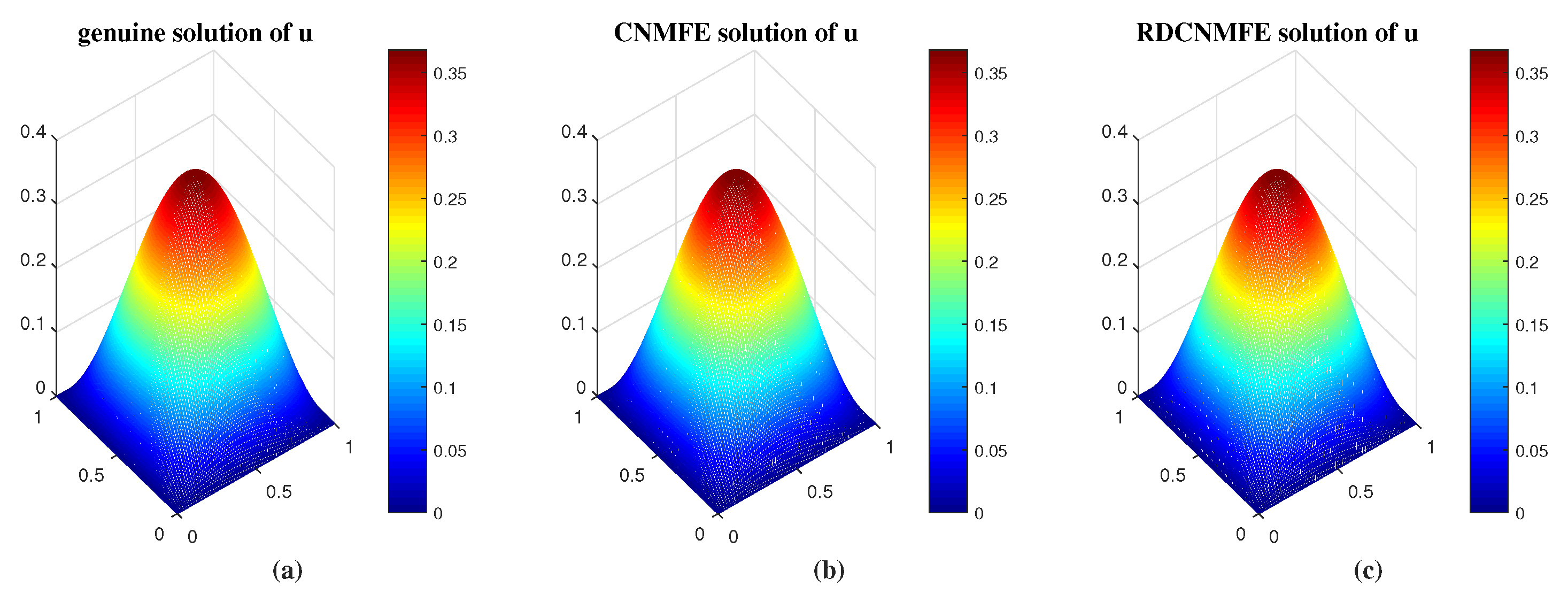
Figure 2.
(a) The genuine solution at t=1. (b) The CNMFE solution at t=1. (c) The RDCNMFE solution at t=1.
Figure 2.
(a) The genuine solution at t=1. (b) The CNMFE solution at t=1. (c) The RDCNMFE solution at t=1.
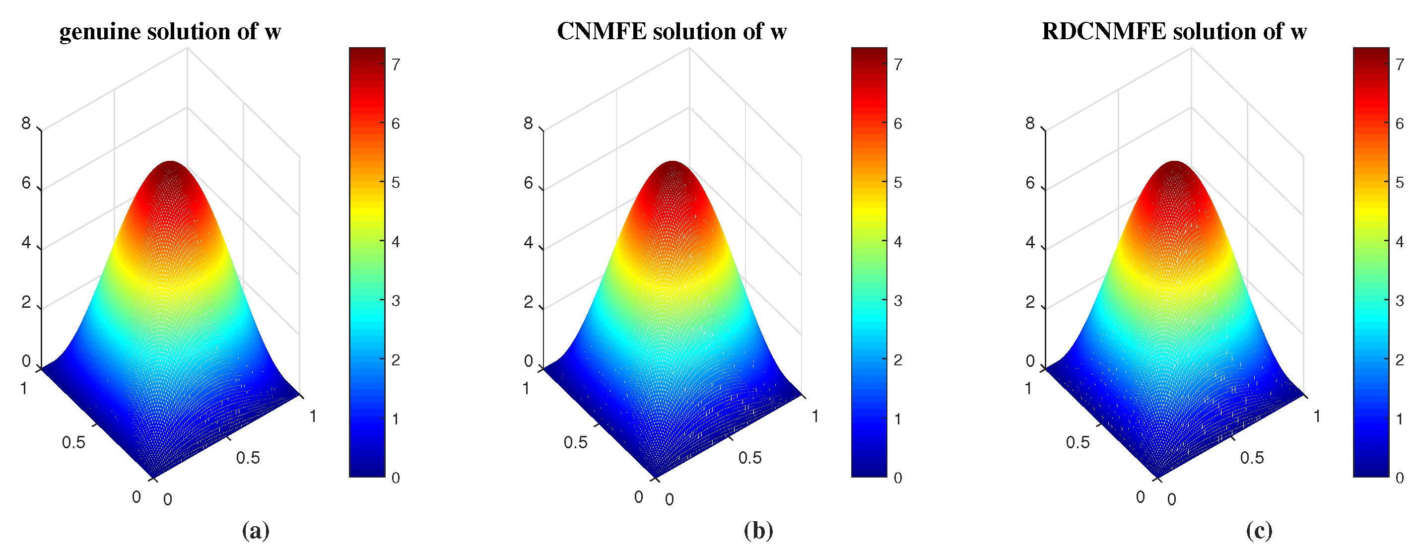
Figure 3.
Comparison of error results of u and .
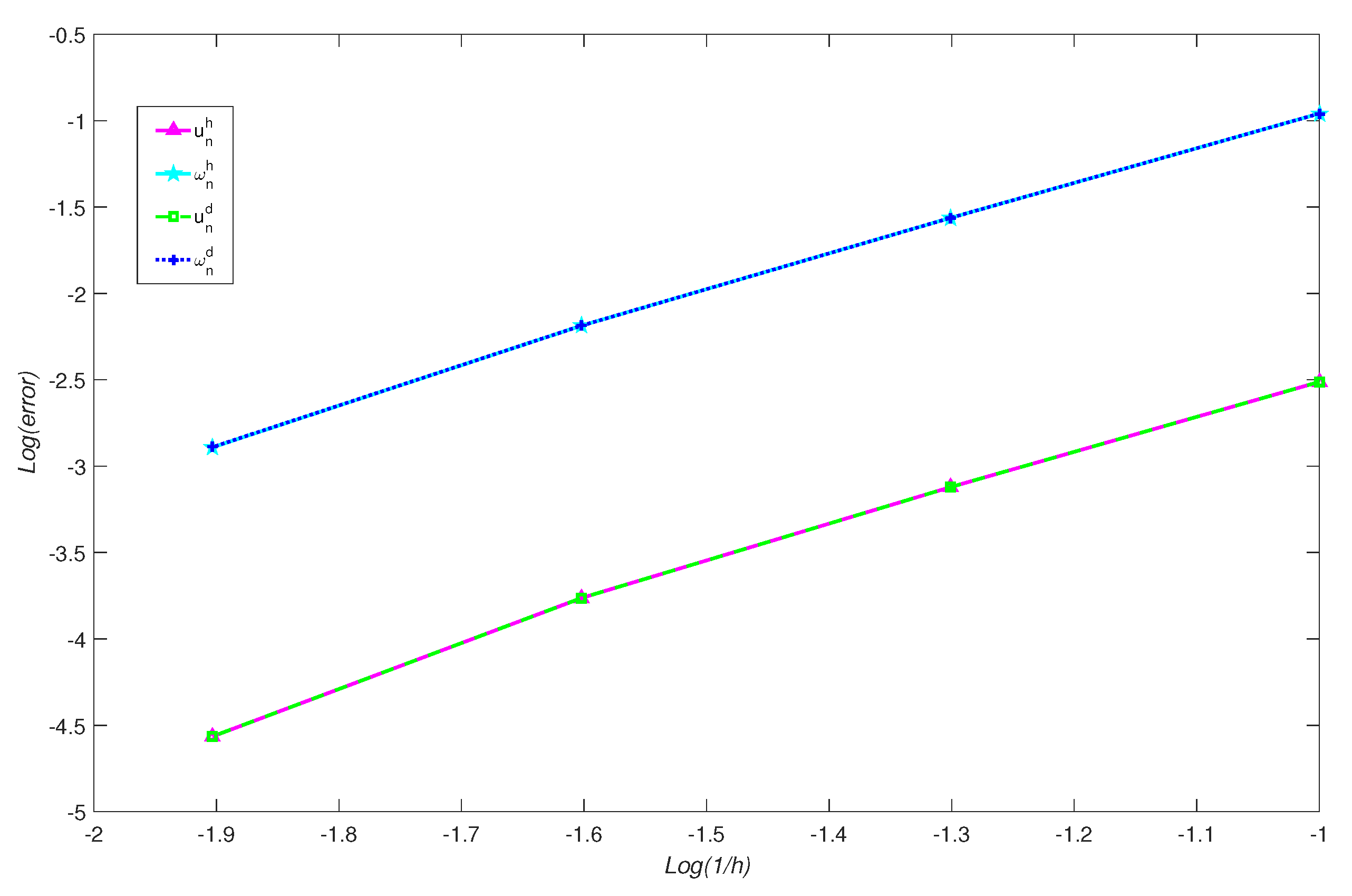

Table 1.
errors and order between the genuine, CNMFE and RDCNMFE solutions of u at t=1.
| CNMFE Method | RDCNMFE Method | |||
|---|---|---|---|---|
| Grid | Order | Order | ||
| 3.0742e-03 | – | 3.0742e-03 | – | |
| 7.5577e-04 | 2.0242 | 7.5577e-04 | 2.0242 | |
| 1.7251e-04 | 2.1313 | 1.7251e-04 | 2.1313 | |
| 2.7256e-05 | 2.6620 | 2.7274e-05 | 2.6611 | |
Table 2.
errors and order between the genuine, CNMFE and RDCNMFE solutions of at t=1.
| CNMFE Method | RDCNMFE Method | |||
|---|---|---|---|---|
| Grid | Order | Order | ||
| 1.0990e-01 | – | 1.0990e-01 | – | |
| 2.7344e-02 | 2.0068 | 2.7344e-02 | 2.0068 | |
| 6.5061e-03 | 2.0714 | 6.5069e-03 | 2.0712 | |
| 1.2863e-03 | 2.3385 | 1.2901e-03 | 2.3345 | |
Table 3.
Comparison of errors and CPU runtime of CNMFE and RDCNMFE solutions.
| CNMFE Method | RDCNMFE Method | |||||
|---|---|---|---|---|---|---|
| Real time | CPU runtime(s) | CPU runtime(s) | ||||
| 2.7256e-05 | 1.2863e-03 | 224.368 | 2.7274e-05 | 1.2901e-03 | 4.410 | |
| 2.5421e-05 | 1.4650e-03 | 260.357 | 4.7928e-05 | 1.4653e-03 | 4.545 | |
| 1.7506e-05 | 1.4287e-03 | 285.453 | 1.7724e-05 | 1.4523e-03 | 4.635 | |
| 1.1089e-05 | 1.3743e-03 | 311.536 | 1.5943e-05 | 1.6888e-03 | 4.678 | |
| 6.8308e-06 | 1.3343e-03 | 342.801 | 6.8312e-06 | 1.3403e-03 | 4.919 | |
Disclaimer/Publisher’s Note: The statements, opinions and data contained in all publications are solely those of the individual author(s) and contributor(s) and not of MDPI and/or the editor(s). MDPI and/or the editor(s) disclaim responsibility for any injury to people or property resulting from any ideas, methods, instructions or products referred to in the content. |
© 2024 by the authors. Licensee MDPI, Basel, Switzerland. This article is an open access article distributed under the terms and conditions of the Creative Commons Attribution (CC BY) license (http://creativecommons.org/licenses/by/4.0/).
Copyright: This open access article is published under a Creative Commons CC BY 4.0 license, which permit the free download, distribution, and reuse, provided that the author and preprint are cited in any reuse.


