
Submitted:
08 July 2025
Posted:
09 July 2025
You are already at the latest version
Abstract
This study presents a novel framework for constructing reduced-order, data-driven twin models for nonlinear partial differential equations, introducing the Koopman Randomized Orthogonal Decomposition (KROD) algorithm for the first time in this context. Compared to classical techniques such as Dynamic Mode Decomposition and Proper Orthogonal Decomposition, the proposed framework offers improved accuracy, efficiency, and interpretability. These improvements are substantiated through rigorous mathematical formalization and analytical validation of the underlying concepts. By integrating randomized SVD with Koopman modal analysis, the approach ensures robust extraction of physically relevant modes and provides a quantitative basis for orthogonal mode computation. The inclusion of explainable deep learning techniques further enhances the model’s transparency and adaptability, with potential for extension to unsupervised learning settings.
Keywords:
data-driven twin model
; Koopman randomized modal decomposition
; nonlinear PDE
; deep learning
1. Introduction
In recent years, digital twin models have emerged as a transformative tool for understanding, simulating, and predicting the behavior of complex physical systems across various domains [1,2,3]. In a broader sense, a digital twin is a virtual representation of a physical system that is continuously updated with real-time data and is capable of capturing the system’s evolution over time [4].
While digital twins have demonstrated considerable utility in the context of engineered systems with well-defined models and sensing infrastructures, their application in replicating nonlinear dynamical systems remains limited by the inherent complexity and nonlinearity of the underlying dynamics. Furthermore, traditional digital twins often require full physical modeling and high computational resources, which limits their scalability and adaptability to purely data-driven or partially observed systems.
To address these challenges, this paper introduces a novel framework, which is termed the data-driven twin model (DTM). This new paradigm is inspired by the digital twin concept but diverges fundamentally in its construction and purpose: rather than embedding a full physics-based model, the data-driven twin model is designed to learn and replicate the nonlinear behavior of a complex dynamical system directly from data with very high fidelity and reduced complexity. Unlike standard machine learning models, which often operate as black boxes, the data-twin model aims to preserve interpretability by decoupling the system’s evolution into a stationary component and a dynamic component in the mathematical framework of modal decomposition [5].
The concept of a data-driven twin model is, to our knowledge, entirely novel and particularly significant in the context of unsupervised learning for dynamical systems. By separating stationary features from time-varying dynamics, the data-twin model facilitates more efficient learning, better generalization to various nonlinear dynamics, and offers insights into the intrinsic structure of the system dynamics. This decomposition is not only beneficial for reducing the learning burden but also opens up new possibilities for transfer learning, system identification, and control.
In this research, the data-driven twin model concept is introduced as a reduced order model that has the main feature to mirror the original process behavior with significantly reduced computational complexity. This advancement addresses a fundamental gap in reduced order modeling: the reconciliation of real-time adaptability with time simulation of nonlinear feature. Associating a nonlinear dynamical process with a data-twin of reduced complexity, assisted by explainable deep learning mathematical tools, has the significant advantage to map the dynamics with highest accuracy and reduced costs in CPU time and hardware to timescales over which that suffers significantly changes and so it could be difficult to explore.
1.1. Modal Decomposition Literature Review and Previous Work
Modal decomposition [5] represents a generic mathematical framework for the characterization of nonlinear dynamical systems in the context of reduced-order modeling [6,7,8,9,10,11,12].
Among the prominent modal decomposition algorithms to produce models of reduced computational complexity, Proper Orthogonal Decomposition and Dynamic Mode Decomposition have become widely adopted in modeling complex dynamical systems.
Proper Orthogonal Decomposition (POD) has its roots in the foundational works of Loéve (1945) and Karhunen (1946) [13,14], who independently developed what is now known as the Karhunen-Loéve (K–L) expansion, a statistical method for representing stochastic processes through orthogonal basis functions. This framework was later extended and formalized in the context of fluid mechanics by Lumley (1970) [15], who introduced POD as a numerical tool for extracting dominant coherent structures from turbulent flow data.
POD has shown effectiveness across a wide range of fields, from turbulent and convection-dominated flows [16,17,18,19] to engineering and oceanography [20,21,22], particularly when combined with data assimilation [23], control [24], or machine learning approaches especially artificial neural networks [25,26,27,28,29]. POD’s reliance on energy-based criteria for selecting basis functions and using truncation-based approximation introduces significant limitations, particularly in the context of highly complex or nonlinear systems. These methods often fail to capture low-energy yet dynamically important modes, leading to reduced accuracy and insufficient representation of critical system behaviors [30,31]. POD suffers also from limited precision in forecasting because it is inherently a projection-based method. By projecting complex, high-dimensional dynamics onto a reduced set of orthogonal modes derived from snapshot data, POD captures only the dominant patterns of variability. As a result, finer scale or transient features, especially those not well represented in the training data, can be lost or poorly reconstructed, leading to reduced accuracy in long-term or highly nonlinear forecasts.
Originally introduced by Koopman (1931), Koopman Operator Theory [32,33] provides a linear, operator-theoretic framework for analyzing and deriving reduced-order models of complex nonlinear dynamical systems. Its modern resurgence began with the pioneering work of Mezić and Banaszuk (2004) in fluid dynamics applications [34,35], laying the foundation for practical, data-driven modal decomposition analysis. Subsequently, Schmid and Sesterhenn (2010) introduced the Dynamic Mode Decomposition (DMD) technique [36,37], a numerical method inspired by Koopman theory that has since been widely adopted across various scientific and engineering disciplines [6,10,38,39]. The research group led by J. Nathan Kutz further advanced the field by developing robust Koopman-based methods for data-driven modeling and system identification [8,40,41,42,43].
Today, Koopman operator theory associated with DMD stands as a central tool in modern dynamical systems analysis and is increasingly recognized as a powerful and influential mathematical framework of the 21st century. The development of numerous DMD variants reflects the ongoing efforts to enhance its robustness and applicability: optimized DMD [44], exact DMD [40], sparsity promoting DMD [45], multi-resolution DMD [42], extended DMD [46], recursive dynamic mode decomposition [47], DMD with control [48], randomized low-rank DMD [49], dynamic mode decomposition with core sketch [50], bilinear dynamic mode decomposition [51], higher order dynamic mode decomposition [52].
DMD captures both spatial and temporal dynamics through modes associated with specific frequencies and growth rates. Yet, standard DMD techniques can suffer from reduced precision if the modes are not selected properly. The accuracy and reliability of the reconstructed or forecasted dynamics heavily depend on identifying the most relevant modes, which is a nontrivial task. Establishing additional mode selection criteria often requires manual tuning, prior knowledge, or heuristic methods, making the process complex and computationally expensive. This not only increases CPU time but also undermines the self-contained nature of the algorithm, limiting its applicability in fully unsupervised learning scenarios.
Author’s contributions have been particularly significant in advancing algorithms based on Koopman operator theory, especially for challenging scenarios involving high-dimensional data and complex temporal behavior. The author has made significant contributions to the development of mode selection strategies in DMD, introducing selection criteria based on amplitude-weighted growth rates and energy-Strouhal number weighting, aimed at systematically extracting the most dynamically relevant modes [53,54].
Moreover, to address the inherent limitations of standard Dynamic Mode Decomposition, specifically, the computational burden of mode selection, the adaptive randomized dynamic mode decomposition (ARDMD) was introduced in [55], offering a more efficient and scalable alternative for extracting dynamic features from high-dimensional data. This innovative algorithm improves efficiency and scalability in reduced-order modeling, particularly in fluid dynamics applications [56].
The techniques introduced in these previous works addressed the persistent challenge of identifying dominant modes in nonlinear and unsteady systems, crucial for accurate reconstruction and forecasting. Author’s work has also extended DMD’s utility into emerging areas like epidemiological modeling [57,58], showcasing its broader societal relevance.
1.2. Novelty and Key Advantages of the Present Research
Recognizing the limitations of standard DMD, particularly the lack of orthogonality and computational cost associated with mode selection, this work proposes a novel framework for constructing reduced-order models of nonlinear dynamical systems. The central objective is to replicate the full system dynamics with significantly lower model complexity, enabling efficient, interpretable, and scalable modeling, i.e. a data-driven twin modeling approach based on modern Koopman operator theory.
In recent years, explainable deep learning has emerged as a preferable alternative to traditional AI approaches that rely on latent variables with unclear or opaque mechanisms. Unlike classical models, whose internal representations often lack interpretability, explainable deep learning provides a framework in which the model’s behavior can be understood, analyzed, and trusted. This work presents an application of explainable deep learning in a controlled, well-understood, and mathematically rigorous setting. The approach not only ensures transparency in the modeling process but also lays a solid foundation for future extensions to unsupervised learning tasks, where the need for reliable and interpretable representations is even more critical.
The core contributions and key advantages include:
1. First mathematical framework for a compact data-driven twin model combining high dynamic fidelity with low computational cost.
2. Fully self-consistent algorithm requiring no heuristic tuning for the reduced-order model parameters.
3. Integration of explainable deep learning for transparent, adaptive modeling in a rigorous, mathematical and controlled setting.
This framework not only improves the interpretability and precision of modal decompositions but also enhances the practical applicability of Koopman operator theory in data-driven modeling.
The structure of the article is organized as follows: Section 2 outlines the mathematical foundations of reduced-order modeling grounded in Koopman operator theory. Section 3 addresses the computational aspects and introduces a novel modal decomposition algorithm, accompanied by a rigorous mathematical justification. Section 4 demonstrates the application of the proposed technique to shock wave phenomena through a series of three experiments of increasing complexity. Section 5 presents the corresponding numerical results. Finally, Section 6 concludes the study with a summary of findings and potential future directions.
2. Mathematical Background
2.1. Computational Complexity Reduction of PDEs by Reduced-Order Modeling
Partial differential equations (PDEs) serve as a fundamental framework for accurately modeling nonlinear dynamical phenomena, owing to their capacity to represent spatial-temporal variations in complex systems. Nevertheless, the numerical solution of PDEs is often computationally demanding, particularly in high-dimensional and strongly nonlinear settings. This computational burden necessitates strategies for complexity reduction to enable practical simulation and analysis. In this context, by reducing the dimensionality of the system while retaining its essential dynamics, reduced-order modeling significantly lowers computational cost and facilitates efficient simulation and analysis.
Suppose that represents the bounded computational domain and let the Hilbert space of square integrable functions on :
to be endowed with the inner product:
and the induced norm for .
Consider a nonlinear PDE for state variable , , , on domain , of the form:
where is a nonlinear differential operator, with the initial condition and Robin boundary conditions given in the following form:
Over the past half-century, partial differential equations have been predominantly solved using numerical techniques such as the finite difference and finite element methods. While these computational tools have significantly advanced our ability to approximate complex PDE solutions, they also introduce substantial implementation complexity and often require a solid understanding of the underlying analytical structure of the equations. In modern computational mathematics, reduced-order modeling has emerged as a powerful approach to mitigate computational demands by simplifying high-dimensional PDE systems, enabling more efficient and tractable solutions without sacrificing essential accuracy.
Definition 1.
The principle of reduced-order modeling aims to finding an approximation solution of the form
which assumes the existence of a basis functions and a locally Lipschitz continuous map , assuring preservation of small global approximation error compared to the true solution of (3) and dynamic stability and computational stability of the reduced-order solution. Expression (6) is called the reduced-order model of the PDE (3).
The basis functions are called modes or shape-functions, therefore the representation (6) is called modal decomposition. Two primary goals are achieved through this modal decomposition approach: (1) the decoupling of spatial structures from the unsteady (time-dependent) components of the solution, and (2) the modeling of the original system’s nonlinearity through a lower-dimensional temporal dynamical system. This separation not only reduces computational complexity but also preserves the essential dynamics of the original PDE system in a more efficient and interpretable form.
2.2. Koopman Operator Framework for Modal Decomposition
Koopman operator theory [32,33,59] offers a rigorous mathematical framework for the modal decomposition of nonlinear dynamical systems by enabling their representation in terms of linear, infinite-dimensional operators acting on observables. In this paper, the Koopman framework is adapted to the context of nonlinear partial differential equations, extending its application to infinite-dimensional dynamical systems governed by PDEs.
Let denote the evolution operator of (3) such that:
i.e., maps the initial condition to the state at time t.
Definition 2.
An observable of the PDE (3) is defined as a possibly nonlinear functional on the state space (e.g., a function space such as )
that maps the infinite-dimensional state u to a measurable quantity.
Remark 1.
The choice of observable g in the Koopman framework is flexible and can range from simple to highly structured representations. A common example is theidentity observable, where , mapping the system state directly to itself. Alternatively, one may consider an infinite-dimensional observable vector, comprising a set of functions of the state, such as
where κ denotes a linear operator (e.g., a differential operator), and the higher-order terms capture nonlinear features of the system. This extended observable space facilitates a richer linear representation of the underlying nonlinear dynamics through the Koopman operator.
Definition 3.
The semigroup of Koopman operators acts on observable functions by composition with the evolution operator of the states:
where is the initial condition.
As a result, the Koopman operator is also known as a composition operator.
In practice, the Koopman operator is considered to be the dual, or more precisely, the left adjoint, of the Ruelle-Perron-Frobenius transfer operator [60,61,62], which acts on the space of probability density functions.
Remark 2.
The Koopman operator is linear, even though the underlying dynamics may be nonlinear:
Remark 3.
The infinitesimal generator of the Koopman semigroup satisfies:
where
and denotes the functional (Fréchet) derivative of g with respect to u, and the inner product is taken over the spatial domain.
Since its introduction in 1931, the operator proposed by Koopman [33,59] remained a purely theoretical construct. In 1985, Lasota and Mackey brought renewed scholarly attention to the Koopman operator [63]. Notably, they were the first to explicitly introduce and formalize the term "Koopman operator" in the literature, thereby establishing a standardized nomenclature for this concept. This terminology was further reinforced in the second edition of their book [64] published in 1994, where the use of the Koopman operator as the adjoint to the Frobenius-Perron operator was maintained and elaborated upon functional analysis in space .
However, at that time, computational resources were still insufficient for the numerical treatment of large-scale complex systems. The practical potential of Koopman Operator Theory began to be realized in the early 2000s. Notably, Mezić and Banaszuk applied it in fluid dynamics [34]. The paper of Mezić [35] is the key modern reference that introduced a rigorous spectral framework for the analysis of nonlinear dynamical systems based on the Koopman operator theory. He formalized the Koopman spectral decomposition, and was the first to introduce the decomposition of observables into Koopman eigenfunctions and associated modes, laying the foundation for a spectral analysis of nonlinear dynamical systems through the Koopman operator framework. The spectral properties of the Koopman operator have been the subject of ongoing investigation, as exemplified in [41,44,65] .
Following Koopman operator theory, the solution can be expressed as a modal decomposition of the form:
where are spatial Koopman modes, and are time-dependent coefficients.
The evolution of the modal coefficients is governed by a possibly nonlinear system:
where is a nonlinear operator that captures the dynamics of the time-dependent coefficients. Thus, the reduced-order solution of form (6) to the PDE is achievable form the perspective of Koopman mode decomposition.
Koopman modes are generally not unique, and their characterization depends on several interrelated factors. First, the definition of Koopman modes is inherently linked to the choice of observables, as the Koopman operator acts on a space of functions rather than directly on the state space. Different selections of observables can lead to different spectral representations, thereby affecting the resulting modes.
This intrinsic non-uniqueness is further compounded in practical settings where Koopman modes are often approximated using numerical techniques such as Dynamic Mode Decomposition (DMD), introduced by P. J. Schmid and J. Sesterhenn in 2008 [36,37]. Such methods introduce additional variability due to factors including data noise, finite sample sizes, and specific algorithmic implementations. Moreover, in cases where the Koopman operator exhibits a degenerate spectrum [10,66], the associated eigenspaces are typically multidimensional, allowing for multiple valid decompositions and further contributing to the non-uniqueness of the Koopman modes.
This paper further introduces a novel algorithm derived from the principles of Dynamic Mode Decomposition, yet fundamentally distinct in its formulation, specifically designed for the construction of a data-driven twin model. This new method computes Koopman modes and their associated temporal coefficients by leveraging the Koopman propagator operator projected onto a Krylov subspace of optimally selected rank. This approach enables a more structured and efficient extraction of spectral components by constraining the dynamics within a finite-dimensional subspace tailored to capture the most relevant features of the system’s evolution.
3. Computational Aspects
This section introduces a novel methodology for constructing a data-driven twin model of a partial differential equation using Koopman mode decomposition. The proposed approach comprises two primary stages. The first stage, referred to as the offline phase, involves the extraction of Koopman modes and the corresponding modal decomposition coefficients that characterize the state evolution of the system. The second stage, known as the online phase, focuses on identifying a nonlinear continuous-time dynamical model that governs the temporal behavior of the data-twin, thereby enabling real-time simulation and prediction. A detailed account of the computational implementation of the proposed methodology is presented hereinafter.
3.1. Offline Phase: Koopman Randomized Orthogonal Decomposition Algorithm
The data , represent measurements of the PDE solution at the constant sampling time , x representing the Cartesian spatial coordinate.
The data matrix whose columns represent the individual data samples is called the snapshot matrix
Each column is a vector with components, representing the spatial measurements corresponding to the time instances.
We aim to find the data-driven twin representation of the solution at every time step , according to the following relation:
where represent the extracted Koopman modes base functions, which we call the leading Koopman modes, represents the number of terms in the representation (17) which we impose to be minimal and represent the modal growing amplitudes.
In classical Dynamic Mode Decomposition the Koopman modes are not orthogonal, which often necessitates a large number of modes to achieve an accurate modal decomposition. This lack of orthogonality represents a significant drawback, as it may lead to redundancy and reduced computational efficiency.
It is more convenient to seek an orthonormal base of Koopman modes
where is the Kronecker delta symbol, consisting of a minimum number of Koopman modes , such that the approximation of through this base is as good as possible, in order to create a data-twin model to the PDE, of reduced computational complexity.
The objective of the present technique is to represent with highest precision the original data through the data-twin model (17) having as few terms as possible. To achieve this goal, several major innovative features are introduced in the proposed algorithm:
- The method produces and extracts orthonormal Koopman modes, ensuring mutual orthogonality among the modes. As a result, a more compact representation is achieved, requiring a smaller number of modes to accurately capture the system dynamics.
- To avoid the computational burden associated with traditional high-dimensional algorithms, the proposed method employs a randomized singular value decomposition (RSVD) technique for dimensionality reduction. The incorporation of randomization offers a key advantage: it eliminates the need for additional selection criteria to identify shape modes, which is typically required in classical approaches such as DMD or POD. The resulting algorithm efficiently identifies the optimal reduced-order subspace that captures the dominant Koopman mode basis, thereby ensuring both computational efficiency and representational fidelity.
- The methodology aims to achieve maximal correlation and minimal reconstruction error between the data-driven twin model and the exact solution of the governing PDE.
The theoretical foundation of randomized singular value decomposition (RSVD) technique was laid in the seminal work of Halko, Martinsson, and Tropp (2011) [67] as part of a broader class of probabilistic algorithms for matrix approximation. Subsequent study of Erichson and Donovan (2016), demonstrated its practical efficiency in motion detection [49]. Bistrian and Navon (2017) extended its use for the first time in fluid dynamics [55,56]. Recently, the theory of randomization has been further employed in the development of reduced-order modeling techniques, particularly in conjunction with projection learning methods [68], block Krylov iteration schemes [69] or deep learning [70].
Proposition 1. (k-RSVD: Randomized Singular Value Decomposition of rank k)
Let be a real-valued data matrix. Having imposed a target rank , the Randomized Singular Value Decomposition of rank k (k-RSVD) produces k left/right singular vectors of and , respectively, and has the following steps:
- 1.
- Generate a Gaussian random test matrix M of size .
- 2.
- Compute a compressed sampling matrix by multiplication of data matrix with random matrix .
- 3.
- Project the data matrix to the smaller space , where H denotes the conjugate transpose.
- 4.
- Produce the economy-size singular value decomposition of low-dimensional data matrix .
- 5.
- Compute the right singular vectors , , , .
Theorem 1. (Koopman Randomized Orthogonal Decomposition)
Let the snapshot matrix (16) containing the PDE solution states be recast into two time-shifted data matrices, whose columns are data snapshots:
For a target rank , the state solution of PDE has the following reduced k-order representation:
on the subspace spanned by the sequence of orthonormal Koopman modes:
where U represents the matrix of left singular vectors produced by k-RSVD of data matrix and X denotes the eigenvectors to the Gram matrix of discrete Koopman propagator operator , i.e. .
The modal temporal coefficients are obtained as scalar products between data snapshots and Koopman modes:
The proposed modal representation method is hereafter referred to as Koopman Randomized Orthogonal Decomposition (KROD).
Proof.
Following the Koopman decomposition assumption [32], a Koopman propagator operator exists, that maps every column vector onto the next one, i.e.
The sequence (23) lies in the Krylov subspace
that captures how the observable evolves under the Koopman dynamics.
The Krylov subspace (24) gives a finite-dimensional proxy to study the action of the infinite-dimensional Koopman operator. For a sufficiently long sequence of the snapshots, suppose that the last snapshot can be written as a linear combination of previous vectors, on the Krylov subspace (24), such that:
in which and is the residual vector. The following relations are true:
where is the unknown column vector.
Assume a diagonal matrix exists that asymptotically approximates the eigenvalues of as approaches zero. Solving the eigenvalue problem:
is equivalent to solve the minimization problem:
where is the -norm of .
For , we identify the k-RSVD of , that yields the factorization:
where and are orthogonal matrices that contain the eigenvectors of and , respectively, is a square diagonal matrix containing the singular values of and H means the conjugate transpose.
Relations and yield:
As a consequence, the solution to the minimization problem (28) is the matrix operator:
As a direct result, the eigenvalues of will converge toward the eigenvalues of the Koopman propagator operator .
Let , be the eigenvectors, respectively the eigenvalues of the Hermitian positive semi-definite Gram matrix :
From the k-RSVD of , it follows that the column space of is the same as the column space of U, i.e.,
Using the definition and substituting into the expression for :
since .
Since is diagonal and W is unitary, represents a unitary similarity transform [71] of matrix , i.e. acts in a reduced coordinate system defined by the k-RSVD.
Let
Since the columns of X are vectors in and U is an orthonormal basis for the column space of , the columns of are linear combinations of the columns of U.
Thus,
i.e. the set of vectors lies in the column space of . Therefore, the span of the eigenvectors forms a subspace of the space containing the data in .
It follows that there exists a subspace of the space containing the data in , spanned by the sequence of Koopman modes:
where U represents the matrix of left singular vectors produced by k-RSVD of data matrix .
We proceed to demonstrate that the columns of are orthonormal. Since U comes from the k-RSVD of , it has orthonormal columns:
Now compute the inner product of :
So the orthonormality of depends on . The matrix X contains the eigenvectors of the Hermitian Gram matrix . Since is Hermitian, it has a complete set of orthonormal eigenvectors. Thus, by choosing the eigenvectors to be orthonormal, we have:
i.e. columns of are orthonormal.
It follows that:
i.e., Koopman modes form an orthnormal base to the data space.
We continue by establishing the formula for the modal coefficients.
Assume that the data evolves linearly in reduced k-order representation (20), written in matrix formulation:
Multiplying both sides on the left by results:
Since has orthonormal columns, we get:
Thus:
If , and , then we can alternatively write:
We choose to project onto the subspace spanned by the orthonormal basis to reduce computational complexity. Consequently, the coefficient matrix
provides a representation with a smaller approximation error in the least-squares sense. □
Proposition 2.
Given a set of integer target ranks and N triples:
each triple encodes a Koopman modes basis, a modal amplitude set, and a corresponding target rank for the reduced k-order representation of the PDE solution, in form of Eq.(20).
Let be the set of all N reduced-order solutions and u be the true PDE solutions.
Determination of the optimal triple to generate the data-twin model is achieved through a constrained multi-objective optimization framework designed to balance model fidelity with consistency to the reference dynamics:
where H denotes the conjugate transpose, and the notation typically denotes the Euclidean norm for vectors, or the Frobenius norm when the state solution of the partial differential equation resides in a space of dimension higher than two.
The optimal triple consists of the Koopman leading modes, the associated modal amplitudes and the rank of the Koopman basis, i.e. the number of terms in Koopman randomized orthogonal decomposition in form:
The optimization problem (46) is resolved numerically, with the methodology and implementation details provided in a subsequent section.
3.2. Online Phase: Modeling the Data-Twin Temporal Dynamic by Explainable Deep Learning
The calculation step of the modes in the offline phase is performed only once. The data-twin model is not complete without the temporal component. These computations are carried out in the second step, during which the mathematical model is integrated over time. Additionally, if needed, the dynamics of the reduced-order model can be evaluated at any specific time point. For this reason, this step is referred to as the online phase, as it can be executed on demand to simulate the behavior of the original process.
Unlike conventional machine learning models, which typically function as opaque black boxes operating on entire datasets without disentangling underlying factors, a key innovation of this study lies in the explicit modeling of temporal dynamics decoupled from spatial dependencies. This is achieved through the use of explainable deep learning techniques, which offer interpretable insights into the data-twin model’s parameters.
In this work, Nonlinear AutoRegressive models with eXogenous inputs (NLARX) are employed as a novel deep learning-based approach within the domain of nonlinear system identification. Since the emergence of artificial neural networks as numerical tools [72,73], NLARX models have been used for various purposes, ranging from simulation [74], to nonlinear predictive control [75] or higher order nonlinear optimization problems [76,77].
The objective is to identify a dynamical system that effectively captures the nonlinear temporal evolution of the underlying process, expressed in the form:
based on modal temporal coefficients computed by KROD algorithm in the offline phase.
To approximate the system dynamics, the evolution of the state is modeled using the NLARX model structure, which is expressed as:
where is a nonlinear estimator realized by a cascade forward neural network, capturing the underlying nonlinear temporal dependencies and input effects. Here, denotes the number of past output terms, represents the number of past input terms used to predict the current output, and corresponds to the input delay, while captures the modeling error. Each output of the NLARX model described in (49) is determined by regressors, which are transformations of previous input and output values. Typically, this mapping consists of a linear component and a nonlinear component, with the final model output being the sum of these two contributions.
Thus, the NLARX model serves as an empirical approximation of the continuous dynamics , with the neural network mapping implicitly representing the evolution operator of the system, such that:
where is the discrete time step and denotes the modeling error.
Training the NLARX model can be formulated as a nonlinear unconstrained optimization problem, of form:
In this formulation, the training dataset comprises the measured input , while denotes the output generated by the NLARX model. The symbol refers to the norm and represents the parameter vector associated with the nonlinear function .
The NLARX architecture is well-suited for capturing system dynamics by feeding previous network outputs back into the input layer. It also allows for the specification of how many past input and output time steps are necessary to accurately represent the system’s behavior. A critical aspect of effectively applying an NLARX network lies in the careful selection of inputs, input delays, and output delays. The objective is to adjust the network parameters across the entire trajectory to minimize the objective function defined in (51).
The reduced-order data-driven twin model for the PDE solution is obtained in the form:
3.3. Qualitative Analysis of the Data-Driven Twin Model
A qualitative assessment of the orthogonality between the Koopman modes derived using the KROD algorithm proposed in this study can be carried out through the Modal Assurance Criterion (MAC) [78]. The MAC value corresponding to a pair of shape modes is defined as follows:
The values lie within the interval as the leading koopman modes obtained from the KROD algorithm are normalized vectors. In this context, Koopman modes are considered orthogonal if:
The Pearson correlation coefficient is employed to quantify the correlation between the data-twin model solution and the true solution of the partial differential equation, providing a measure of how closely the data-twin model approximates the true dynamics across the space-time domain.
Let be the true solution and be the data-twin model solution of PDE, sampled at spatial points and time instances. Define the flattened vectors:
The Pearson correlation coefficient between and is given by:
where
In addition to the Pearson correlation coefficient, the mean absolute error (MAE) is employed as a complementary metric to assess the average magnitude of pointwise discrepancies over the space-time domain, providing a more direct measure of predictive accuracy irrespective of correlation structure:
In addition to these metrics, to provide fine-grained, pointwise insight into how well the data-twin model approximates the true solution of PDE at specific locations in space and time, we define the absolute local error matrix as:
for all and .
3.4. Time Simulation and Validation of the Data-Driven Twin Model
Data-driven twin model is subjected to time-domain simulation, followed by a two-step input-output validation of its predicted response. In the first validation step, the model is trained using the initial two-thirds of the available snapshots, with the remaining one-third reserved for validation. In the subsequent step, the training dataset is further reduced to the first one-third of the snapshots, and the remaining two-thirds are employed to assess the model’s predictive performance.
4. Data-Driven Twin Modeling of Shock Wave Phenomena Using KROD
This section demonstrates the application of the proposed KROD algorithm to shock wave modeling using the viscous Burgers’ equation.
4.1. Governing Equations of the Mathematical Model
The viscous Burgers equation model is considered, of the form:
where is the unknown function of time t, is the viscosity parameter.
Three experiments are considered, exhibiting progressively more complex dynamics, each characterized by an initial condition of the following form:
Homogeneous Dirichlet boundary conditions are imposed for all three examples, specified as follows:
Equation (59), which defines the initial condition for Experiment 1, produces a sinusoidal pulse characterized by an abrupt change in slope at the boundaries of the domain. The initial value problem with the discontinuous initial condition given by (60) is referred to as a Riemann problem, which leads to the formation of a shock wave. For Experiment 3, the initial condition described by (61) induces a more complex evolution of the pulse. All three experiments involve phenomena that pose significant challenges for standard numerical methods to accurately capture.
4.2. Derivation of the Analytical Solution Using the Cole-Hopf Transformation
The Cole-Hopf transformation is defined by
Through analytical treatment, it is found that:
Substituting these expressions into (58) it follows that:
Relation (66) indicates that if solves the heat equation, then given by the Cole-Hopf transformation (Section 4.2) solves the viscous Burgers equation (58). Thus the viscous Burgers equation (58) is recast into the following one:
Taking the Fourier transform with respect to x for both heat equation and the initial condition (67) it is found that:
Using the Cole-Hopf transformation (Section 4.2), the analytic solution to the problem (58) is obtained in the following form:
4.3. Derivation of the Numerical Exact Solution Using the Gauss-Hermite Quadrature
To compute the exact solution (69) corresponding to the initial conditions of the three test cases (59)–(61), the Gauss-Hermite quadrature technique [81] is employed.
Gauss–Hermite quadrature approximates the value of integrals of the following kind:
where n represents the number of sample points used, are the roots of the Hermite polynomial and the associated weights are given by
In Experiment 1, the initial condition is defined by Eq.(59):
and the exact solution (69) is in form:
With the variable change:
the exact solution to the Burgers equation model (58) with the initial condition (59) is equivalent with the following form:
Similarly, by applying the variable transformation (74), the exact solutions for the subsequent two experiments are derived as follows.
In the case of Experiment 2 the exact solution to the Burgers equation model (58) with the initial condition (60) is:
In the case of Experiment 3 the exact solution to the Burgers equation model (58) with the initial condition (61) is:
To obtain the numerical exact solutions for the three test cases, both the numerator and denominator are evaluated using Gauss-Hermite quadrature (70).
5. Numerical Results
The following section presents numerical results demonstrating the computational performance of the Koopman Randomized Orthogonal Decomposition (KROD) method introduced in this study, in conjunction with Deep Learning (DL) for time simulation. It is shown that the resulting output is a high-fidelity, reduced-complexity model that effectively replicates the behavior of the original system and enables real-time simulation with high accuracy, thereby producing a data-driven twin model.
The computational domain is defined as , with , and the time interval considered is , where . The viscosity parameter in the Burgers equation is set to for all three experiments. The domain is uniformly discretized using grid points, resulting in a mesh size of .
The Riemann problem parameters are assumed to be and .
By applying the Cole-Hopf transformation (Section 4.2), the analytical solutions to the Burgers problem (58) are obtained for all three experiments, corresponding respectively to the forms (75), (76), and (77), as detailed in Section 4.2. Subsequently, the exact solutions for the three test cases are computed numerically using the Gauss-Hermite quadrature method (70) with nodes (see Section 4.3).
Figure 1 presents the exact solutions for the three experiments under consideration.
The data-driven twin models of the form (47) are generated using the Koopman Randomized Orthogonal Decomposition (KROD) algorithm as high-fidelity surrogates for the three Burgers problems examined in this study. For this purpose, the training dataset consists of a total of snapshots collected at uniformly spaced time intervals of , and spatial measurements recorded for each time snapshot.
KROD algorithm determines the optimal dimension of the subspace spanned by the dominant Koopman modes by solving the multiobjective optimization problem with nonlinear constraints stated in (46). This problem is solved by employing a genetic algorithm to identify the Pareto front corresponding to the two fitness functions.
Figure 2 depicts the optimization objectives defined in (46) along with the Pareto front solutions for each of the three experiments.
For Experiment 1, the dimension of the subspace spanned by the leading modes is . In Experiment 2, the data-twin model representing the Riemann problem dynamics has a subspace dimension of . For Experiment 3, the increased complexity of the pulse is captured by a data-twin model with a higher dimension of . In all three cases, the computational time required by the KROD algorithm in offline phase remains extremely low, as illustrated in Figure 3.
KROD algorithm identifies the optimal dimension of the modal basis and computes the optimal Koopman modes along with their associated time-dependent amplitudes. As a result, the data-driven twin model (47) is constructed, which-by definition-exhibits minimal approximation error and maximal correlation with respect to the original data model.
To facilitate a qualitative assessment of the DTMs, Table 1 reports the outcomes of the multiobjective optimization problem (46) as solved by the KROD. Specifically, the table includes the dimensionality of the leading Koopman modes, the absolute error as defined in Eq. (56), and the correlation coefficient as given by Eq. (55) between the exact solution and the corresponding data-twin model for each of the three experiments considered.
An analysis of the results presented in Table 1 reveals that KROD algorithm produces models exhibiting perfect correlation with the original data, i.e., , across all three test cases. Furthermore, the absolute errors remain remarkably low, on the order of .
The selection of modes solely based on their energy ranking proves effective only under specific conditions [47,82]. Some modes, despite contributing minimally to the overall energy, may exhibit rapid temporal growth at low amplitudes or represent strongly damped high-amplitude structures. Such modes can play a significant role in enhancing the fidelity of the data-twin model. A key advantage of the KROD algorithm over traditional DMD-based approaches lies in its ability to generate a substantially lower-dimensional subspace that retains the most dynamically significant Koopman modes. As a result, the KROD method avoids the need for an additional-often subjective-mode selection criterion. Moreover, the orthogonality of the KROD modes contributes to their qualitative superiority, enabling accurate modeling with a reduced number of modes.
To assess the orthogonality of the Koopman modes computed by KROD algorithm, the orthogonality matrix introduced in Section 3.3 is evaluated for each of the three experiments considered in this study. The following figures display the computed values for each pair of leading shape modes, as defined previously in Eq. (53).
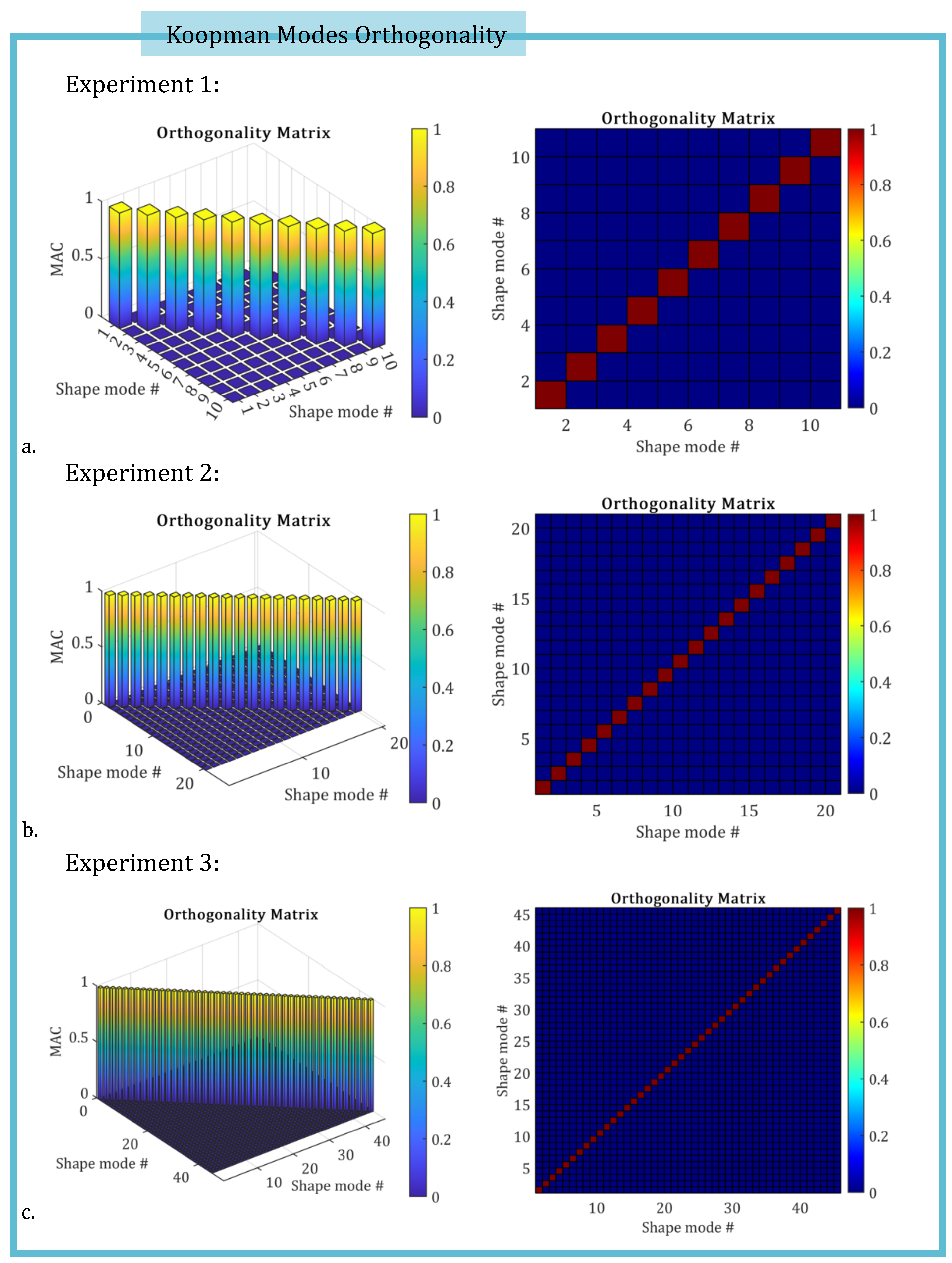
Figure 4.
The orthogonality matrices corresponding to the three investigated experiments are shown, respectively. The values, computed according to Eq. (53), confirm the mutual orthogonality of the Koopman modes in each case.
Figure 4.
The orthogonality matrices corresponding to the three investigated experiments are shown, respectively. The values, computed according to Eq. (53), confirm the mutual orthogonality of the Koopman modes in each case.
The KROD algorithm facilitates the identification of the leading Koopman modes and their corresponding temporal coefficients. To achieve high-fidelity time simulation of the data-driven twin model’s temporal parameters, Nonlinear AutoRegressive models with eXogenous inputs (NLARX) are employed (revise Subsection (Section 3.4). Figure 5, Figure 6 and Figure 7 present the two-fold input-output validation results for three randomly selected temporal coefficients, simulated using the optimal NLARX models for Experiments 1, 2, and 3, respectively. These results demonstrate that the deep learning-based NLARX models accurately replicate the coefficient dynamics, even when the training dataset is reduced to only the first third of the available snapshots. Relevant performance metrics for the deep learning simulations are also provided in the figures.
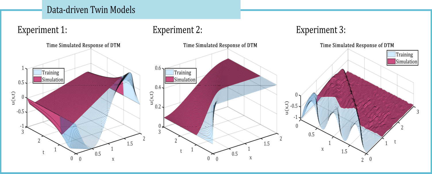
The time-simulated data-driven twin models are assembled in the form specified by Eq. (52) for each of the three experiments considered. The output responses are then compared to the corresponding exact solutions in terms of absolute local error given by Eq. (57), as illustrated in Figure 8.
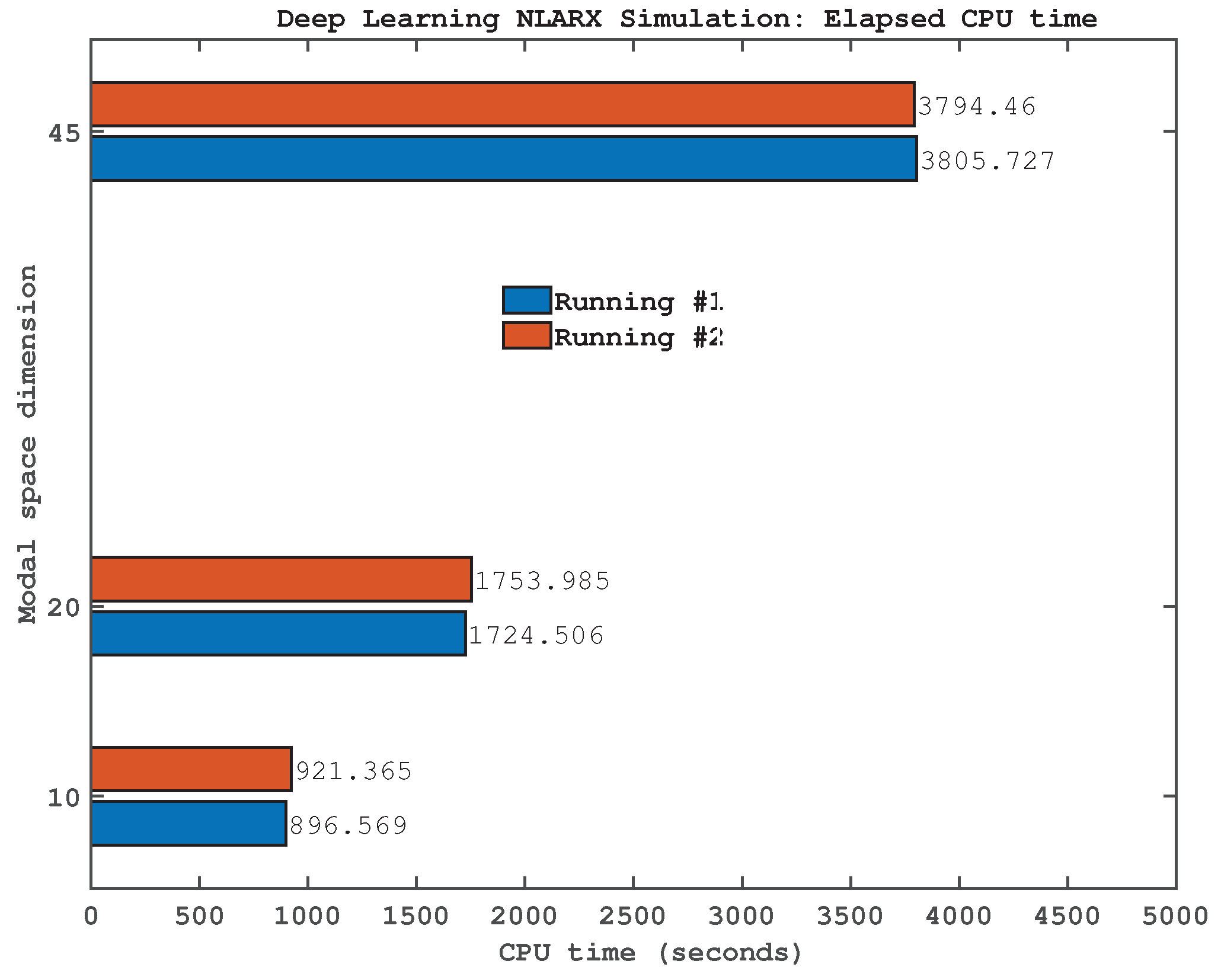
Figure 9 presents the CPU time required during the online phase of the algorithm, in which the deep learning process is executed, as a function of the optimized modal space dimension for the three experimental cases analyzed. The reported CPU times correspond to two successive computational runs. All simulations and visualizations were performed using custom scripts developed in Matlab R2022a and executed on a system equipped with an Intel i7-7700K processor. The observed computational times are considered acceptable and fall within a reasonable range for practical implementation.
6. Conclusions
This study introduces a novel framework for constructing data-driven twin models of reduced computational complexity for partial differential equations models, a topic of significant relevance in data science. To our knowledge, this work is the first to introduce the Koopman Randomize Orthogonal Decomposition (KROD) algorithm within the context of nonlinear PDEs.
The proposed approach consists of two main phases. Initially, a new numerical algorithm is developed to generate a reduced-order data-twin model based on the KROD decomposition of the data. Subsequently, explainable NLARX Deep Learning technique is employed to enable real-time, adaptive calibration of the data-twin model and to compute its dynamic response.
The resulting twin data model exhibits minimal error and maximal correlation with the original dataset, offering a highly accurate and computationally efficient representation of the underlying physical system.
This study introduces several methodological advancements that distinguish it from classical modal decomposition techniques such as Dynamic Mode Decomposition and Proper Orthogonal Decomposition, which often depend on heuristic or ad hoc criteria for mode selection. In contrast, the proposed Randomized Koopman Orthogonal Decomposition leverages randomized singular value decomposition to substantially reduce computational cost while fully automating the selection of dominant modes.
Building upon the author’s earlier work [55,56,70], it is shown that the stochastic nature of RSVD inherently favors the most relevant modes, thereby enhancing robustness without introducing additional algorithmic complexity.
A key novelty lies in the first quantitative framework for computing orthogonal Koopman modes using randomized orthogonal projections, which ensures optimal representation in the data space. Moreover, the proposed method integrates explainable deep learning techniques within the modal decomposition process, enabling interpretable and real-time calibration of the reduced-order data-twin model. This integration also provides a pathway for future extensions into unsupervised learning paradigms.
Importantly, the framework is inherently compatible with unsupervised learning, functioning effectively on raw observational data without requiring predefined models. This characteristic promotes broader applicability and generalization across a wide range of fluid dynamics problems and complex dynamical systems. The specific application of the KROD methodology to fluid dynamics will be addressed in future investigations.
Conflicts of Interest
The author declares no conflict of interest.
Abbreviations
The following abbreviations are used in this manuscript:
| DTM | Data-driven Twin Model |
| KROD | Koopman Randomized Orthogonal Decomposition |
| POD | Proper Orthogonal Decomposition |
| DMD | Dynamic Mode Decomposition |
| PDE | Partial Differential Equation |
| NLARX | Nonlinear AutoRegressive models with eXogenous inputs |
References
- Grieves, M.; Vickers, J. Digital twin: Mitigating unpredictable, undesirable emergent behavior in complex systems. Transdisciplinary Perspectives on Complex Systems 2017, 85–113. [Google Scholar]
- Tao, F.; Zhang, M.; Liu, Y.; Nee, A.Y.C. Digital twin in industry: State-of-the-art. IEEE Transactions on Industrial Informatics 2019, 15, 2405–2415. [Google Scholar] [CrossRef]
- Glaessgen, E.; Stargel, D. The digital twin paradigm for future NASA and U.S. Air Force vehicles. In Proceedings of the 53rd AIAA/ASME/ASCE/AHS/ASC Structures, Structural Dynamics and Materials Conference, 2012.
- Rasheed, A.; San, O.; Kvamsdal, T. Digital Twin: Values, Challenges and Enablers From a Modeling Perspective. IEEE Access 2020, 8, 21980–22012. [Google Scholar] [CrossRef]
- Holmes, P.; Lumley, J.; Berkooz, G. Turbulence, coherent structures, dynamical systems and symmetry; Cambridge Univ. Press, 1996.
- Rowley, C.W.; Mezić, I.; Bagheri, S.; Schlatter, P.; Henningson, D.S. Reduced-order models for flow control: balanced models and Koopman modes. In Proceedings of the Seventh IUTAM Symposium on Laminar-Turbulent Transition, IUTAM Bookseries. Seventh IUTAM Symposium on Laminar-Turbulent Transition, IUTAM Bookseries, 2010, Vol. 18, pp. 43–50.
- Frederich, O.; Luchtenburg, D.M. Modal analysis of complex turbulent flow. In Proceedings of the The 7th International Symposium on Turbulence and Shear Flow Phenomena (TSFP-7), Ottawa, Canada, July 28-31 2011. [Google Scholar]
- Kutz, J.; Sashidhar, D.; Sahba, S.; Brunton, S.; McDaniel, A.; Wilcox, C. Physics-informed machine-learning for modeling aero-optics. In Proceedings of the International Conference On Applied Optical Metrology, 2021, Vol. 4, pp. 70–77.
- Schmid, P.J.; Violato, D.; Scarano, F. Decomposition of time-resolved tomographic PIV; Springer-Verlag, 2012.
- Mezić, I. Koopman Operator, Geometry, and Learning of Dynamical Systems. Notices of the American Mathematical Society 2021, 68, 1087–1105. [Google Scholar] [CrossRef]
- Ahmed, S.E.; San, O.; Bistrian, D.A.; Navon, I.M. Sampling and resolution characteristics in reduced order models of shallow water equations: Intrusive vs nonintrusive. International Journal for Numerical Methods in Fluids 2020, 92, 992–1036. [Google Scholar] [CrossRef]
- Xiao, D.; Fang, F.; Heaney, C.E.; Navon, I.M.; Pain, C.C. A domain decomposition method for the non-intrusive reduced order modelling of fluid flow. Computer Methods in Applied Mechanics and Engineering 2019, 354, 307–330. [Google Scholar] [CrossRef]
- Karhunen, K. Zur spektral theorie stochastischer prozesse. Annu. Acad. Sci. Fennicae Ser.A, J. Math. Phys. 1946, 34, 1–7. [Google Scholar]
- Loéve, M. Sur la covariance d’une fonction aleatoire. C. R. Acad. Sci. Paris 1945, 220, 295–296. [Google Scholar]
- Lumley, J.L. Stochastic Tools in Turbulence; Academic Press New York, 1970.
- Iliescu, T. ROM Closures and Stabilizations for Under-Resolved Turbulent Flows. In Proceedings of the 2022 Spring Central Sectional Meeting, 2022.
- Wang, Z.; Akhtar, I.; Borggaard, J.; Iliescu, T. Proper orthogonal decomposition closure models for turbulent flows: A numerical comparison. Computer Methods in Applied Mechanics and Engineering 2012, 10, 237–240. [Google Scholar] [CrossRef]
- Xiao, D.; Heaney, C.E.; Fang, F.; Mottet, L.; Hu, R.; Bistrian, D.A.; Aristodemou, D.; Navon, I.M.; Pain, C.C. A domain decomposition non-intrusive reduced order model for turbulent flows. Computers and Fluids 2019, 182, 15–27. [Google Scholar] [CrossRef]
- Gunzburger, M.; Iliescu, T.; Mohebujjaman, M.; Schneier, M. Nonintrusive stabilization of reduced order models for uncertainty quantification of time-dependent convection-dominated flows. Preprint arXiv 2018, arXiv:1810.08746. [Google Scholar]
- San, O.; Staples, A.; Wang, Z.; Iliescu, T. Approximate deconvolution large eddy simulation of a barotropic ocean circulation model. Ocean Modelling 2011, 40, 120–132. [Google Scholar] [CrossRef]
- San, O.; Iliescu, T. A stabilized proper orthogonal decomposition reduced-order model for large scale quasigeostrophic ocean circulation. Advances in Computational Mathematics 2014, 41, 1289–1319. [Google Scholar] [CrossRef]
- Osth, J.; Noack, B.R.; Krajnovic, S.; Barros, D.; Boree, J. On the need for a nonlinear subscale turbulence term in POD models as exemplified for a high-Reynolds-number flow over an Ahmed body. Journal of Fluid Mechanics 2014, 747, 518–544. [Google Scholar] [CrossRef]
- Xiao, D.; Du, J.; Fang, F.; Pain, C.; Li, J. Parameterised non-intrusive reduced order methods for ensemble Kalman filter data assimilation. Computers and Fluids 2018, 177. [Google Scholar] [CrossRef]
- Sierra, C.; Metzler, H.; Muller, M.; Kaiser, E. Closed-loop and congestion control of the global carbon-climate system. Climatic Change 2021, 165, 1–24. [Google Scholar] [CrossRef]
- Xiao, D.; Heaney, C.E.; Mottet, L.; Fang, F.; Lin, W.; Navon, I.M.; Guo, Y.; Matar, O.K.; Robins, A.G.; Pain, C.C. A reduced order model for turbulent flows in the urban environment using machine learning. Building and Environment 2019, 148, 323–337. [Google Scholar] [CrossRef]
- San, O.; Maulik, R.; Ahmed, M. An artificial neural network framework for reduced order modeling of transient flows. Communications in Nonlinear Science and Numerical Simulation 2019, 77, 271–287. [Google Scholar] [CrossRef]
- Kaptanoglu, A.; Callaham, J.; Hansen, C.; Brunton, S. Machine Learning to Discover Interpretable Models in Fluids and Plasmas. Bulletin of the American Physical Society 2022. [Google Scholar]
- Owens, K.; Kutz, J. Data-driven discovery of governing equations for coarse-grained heterogeneous network dynamics. SIAM Journal on Applied Dynamical Systems 2023, 22. [Google Scholar] [CrossRef]
- Cheng, M.; Fang, F.; Pain, C.; Navon, I. Data-driven modelling of nonlinear spatio-temporal fluid flows using a deep convolutional generative adversarial network. Computer Methods in Applied Mechanics and Engineering 2020, 365, 113000. [Google Scholar] [CrossRef]
- Dumon, A.; Allery, C.; Ammar, A. Proper Generalized Decomposition method for incompressible Navier-Stokes equations with a spectral discretization. Applied Mathematics and Computation 2013, 219, 8145–8162. [Google Scholar] [CrossRef]
- Dimitriu, G.; Ştefănescu, R.; Navon, I.M. Comparative numerical analysis using reduced-order modeling strategies for nonlinear large-scale systems. Journal of Computational and Applied Mathematics 2017, 310, 32–43. [Google Scholar] [CrossRef]
- Koopman, B. Hamiltonian systems and transformations in Hilbert space. Proc. Nat. Acad. Sci. 1931, 17, 315–318. [Google Scholar] [CrossRef] [PubMed]
- Koopman, B.; von Neumann, J. Dynamical systems of continuous spectra. Proc Natl Acad Sci U S A. 1932, 18, 255–263. [Google Scholar] [CrossRef]
- Mezić, I.; Banaszuk, A. Comparison of systems with complex behavior. Physica D: Nonlinear Phenomena 2004, 197, 101–133. [Google Scholar] [CrossRef]
- Mezić, I. Spectral properties of dynamical systems, model reduction and decompositions. Nonlinear Dynamics 2005, 41, 309–325. [Google Scholar] [CrossRef]
- Schmid, P.J.; Sesterhenn, J. Dynamic mode decomposition of numerical and experimental data. In Proceedings of the 61st Annual Meeting of the APS Division of Fluid Dynamics, American Physical Society, San Antonio, Texas, November 2008. Vol. 53(15). [Google Scholar]
- Schmid, P. Dynamic mode decomposition of numerical and experimental data. Journal of Fluid Mechanics 2010, 656, 5–28. [Google Scholar] [CrossRef]
- Percic, M.; Zelenika, S.; Mezić, I. Artificial intelligence-based predictive model of nanoscale friction using experimental data. Friction 2021, 9, 1726–1748. [Google Scholar] [CrossRef]
- Pant, P.; Doshi, R.; Bahl, P.; Farimani, A.B. Deep learning for reduced order modelling and efficient temporal evolution of fluid simulations. Physics of Fluids 2021, 33, 107101. [Google Scholar] [CrossRef]
- Tu, J.H.; Rowley, C.W.; Luchtenburg, D.M.; Brunton, S.L.; Kutz, J.N. On dynamic mode decomposition: Theory and applications. Journal of Computational Dynamics 2014, 1, 391–421. [Google Scholar] [CrossRef]
- Brunton, S.L.; Brunton, B.W.; Proctor, J.L.; Kutz, J.N. Koopman Invariant Subspaces and Finite Linear Representations of Nonlinear Dynamical Systems for Control. PLoS ONE 2016, 11, e0150171. [Google Scholar] [CrossRef] [PubMed]
- Kutz, J.N.; Fu, X.; Brunton, S.L. Multiresolution dynamic mode decomposition. SIAM Journal on Applied Dynamical Systems 2016, 15, 713–735. [Google Scholar] [CrossRef]
- Li, B.; Ma, Y.; Kutz, J.; Yang, X. The Adaptive Spectral Koopman Method for Dynamical Systems. SIAM Journal on Applied Dynamical Systems 2023, 22, 1523–1551. [Google Scholar] [CrossRef]
- Chen, K.K.; Tu, J.H.; Rowley, C.W. Variants of dynamic mode decomposition: boundary condition, Koopman and Fourier analyses. Nonlinear Science 2012, 22, 887–915. [Google Scholar] [CrossRef]
- Jovanovic, M.R.; Schmid, P.J.; Nichols, J.W. Sparsity-promoting dynamic mode decomposition. Physics of Fluids 2014, 26, 024103. [Google Scholar] [CrossRef]
- Williams, M.O.; Kevrekidis, I.G.; Rowley, C.W. A data-driven approximation of the Koopman operator: extending Dynamic Mode Decomposition. Nonlinear Science 2015, 25, 1307–1346. [Google Scholar] [CrossRef]
- Noack, B.R.; Stankiewicz, W.; Morzynski, M.; Schmid, P.J. Recursive dynamic mode decomposition of transient and post-transient wake flows. Journal of Fluid Mechanics 2016, 809, 843–872. [Google Scholar] [CrossRef]
- Proctor, J.L.; Brunton, S.L.; Kutz, J.N. Dynamic mode decomposition with control. SIAM Journal of Applied Dynamical Systems 2016, 15, 142–161. [Google Scholar] [CrossRef]
- Erichson, N.B.; Donovan, C. Randomized low-rank Dynamic Mode Decomposition for motion detection. Computer Vision and Image Understanding 2016, 146, 40–50. [Google Scholar] [CrossRef]
- Ahmed, S.E.; Dabaghian, P.H.; San, O.; Bistrian, D.A.; Navon, I.M. Dynamic mode decomposition with core sketch. Physics of Fluids 2022, 34, 066603. [Google Scholar] [CrossRef]
- Goldschmidt, A.; Kaiser, E.; Dubois, J.; Brunton, S.; Kutz, J. Bilinear dynamic mode decomposition for quantum control. New Journal of Physics 2021, 23, 033035. [Google Scholar] [CrossRef]
- Le Clainche, S.; Vega, J.M. Higher Order Dynamic Mode Decomposition. SIAM Journal on Applied Dynamical Systems 2017, 16, 882–925. [Google Scholar] [CrossRef]
- Bistrian, D.A.; Navon, I.M. An improved algorithm for the shallow water equations model reduction: Dynamic Mode Decomposition vs POD. International Journal for Numerical Methods in Fluids 2015, 78, 552–580. [Google Scholar] [CrossRef]
- Bistrian, D.A.; Navon, I.M. The method of dynamic mode decomposition in shallow water and a swirling flow problem. International Journal for Numerical Methods in Fluids 2017, 83, 73–89. [Google Scholar] [CrossRef]
- Bistrian, D.A.; Navon, I.M. Randomized dynamic mode decomposition for nonintrusive reduced order modelling. International Journal for Numerical Methods in Engineering 2017, 112, 3–25. [Google Scholar] [CrossRef]
- Bistrian, D.A.; Navon, I.M. Efficiency of randomised dynamic mode decomposition for reduced order modelling. International Journal Of Computational Fluid Dynamics 2018, 32, 88–103. [Google Scholar] [CrossRef]
- Bistrian, D.A.; Dimitriu, G.; Navon, I.M. Modeling dynamic patterns from COVID-19 data using randomized dynamic mode decomposition in predictive mode and ARIMA. In Proceedings of the AIP Conference Proceedings, 2020, Vol. 2302, p. 080002.
- Bistrian, D.A.; Dimitriu, G.; Navon, I.M. Processing epidemiological data using dynamic mode decomposition method. In Proceedings of the AIP Conference Proceedings, 2019, Vol. 2164, p. 080002.
- Koopman, B. On distributions admitting a sufficient statistic. Transactions of the American Mathematical Society 1936, 39, 399–400. [Google Scholar] [CrossRef]
- Perron, O. Zur Theorie der Matrices. Mathematische Annalen 1907, 64, 248–263. [Google Scholar] [CrossRef]
- Frobenius, G. Uber Matrizen aus positiven Elementen. Sitzungsberichte der Koniglich Preussischen Akademie der Wissenschaften 1908, 1, 471–476. [Google Scholar]
- Ruelle, D.P. Chance and chaos; Vol. 110, Princeton University Press, 1993.
- Lasota, A.; Mackey, M.C. Probabilistic properties of deterministic systems; Cambridge University Press, 1985.
- Lasota, A.; Mackey, M. Chaos, Fractals, and Noise. Stochastic Aspects of Dynamics; Springer, 1994.
- Rowley, C.W.; Mezić, I.; Bagheri, S.; Schlatter, P.; Henningson, D.S. Spectral analysis of nonlinear flows. Journal of Fluid Mechanics 2009, 641, 115–127. [Google Scholar] [CrossRef]
- Mezić, I. On numerical approximations of the Koopman operator. Mathematics 2022, 10, 1180. [Google Scholar] [CrossRef]
- Halko, N.; Martinsson, P.G.; Tropp, J.A. Finding structure with randomness: Probabilistic algorithms for constructing approximate matrix decompositions. SIAM Review 2001, 53, 217–288. [Google Scholar] [CrossRef]
- Surasinghe, S.; Bollt, E.M. Randomized Projection Learning Method for DynamicMode Decomposition. Mathematics 2021, 9, 1–17. [Google Scholar] [CrossRef]
- Qiu, Y.; Sun, W.; Zhou, G.; Zhao, Q. Towards efficient and accurate approximation: tensor decomposition based on randomized block Krylov iteration. Signal, Image and Video Processing 2024, 18, 6287–6297. [Google Scholar] [CrossRef]
- Bistrian, D.A. High-fidelity digital twin data models by randomized dynamic mode decomposition and deep learning with applications in fluid dynamics. Modelling 2022, 3, 314–332. [Google Scholar] [CrossRef]
- Golub, G.H.; Loan, C.F.V. Matrix Computations (4th edition); Johns Hopkins University Press, 2013.
- Juditsky, A.; Hjalmarsson, H.; Benveniste, A.; Deylon, B.; Ljung, L.; Sloberg, J.; Zhang, Q. Nonlinear black-box models in system identification: Mathematical foundations. Automatica 1995, 31, 1725–1750. [Google Scholar] [CrossRef]
- Ljung, L. System Identification: Theory for the User; Information and System Sciences Series, Prentice Hall, 1999.
- Nelles, O. Nonlinear System Identification: From Classical Approaches to Neural Networks and Fuzzy Models; Springer, 2001.
- Liu, G.; Kadirkamanathan, V.; Billings, S. Predictive control for non-linear systems using neural networks. International Journal of Control 1998, 71, 1119–1132. [Google Scholar] [CrossRef]
- Tieleman, T.; Hinton, G. Divide the gradient by a running average of its recent magnitude; COURSERA: Neural Networks for Machine Learning, 2012.
- Wang, Z.; Xiao, D.; Fang, F.; Govindan, R.; Pain, C.; Guo, Y. Model identification of reduced order fluid dynamics systems using deep learning. International Journal for Numerical Methods in Fluids 2018, 86, 255–268. [Google Scholar] [CrossRef]
- Ewins, D. Modal Testing: Theory, Practice and Application; Research Studies Press Ltd., 2000.
- Hopf, E. The partial differential equation ut + uux = νuxx. Communications on Pure and Applied Mathematics 1950, 3, 201–230. [Google Scholar] [CrossRef]
- Cole, J.D. On a quasi-linear parabolic equation occurring in aerodynamics. Quarterly of Applied Mathematics 1951, 9, 225–236. [Google Scholar] [CrossRef]
- Brass, H.; Petras, K. Quadrature Theory. The Theory of Numerical Integration on a Compact Interval; American Mathematical Society, 2011.
- Noack, B.R.; Morzynski, M.; Tadmor, G. Reduced-Order Modelling for Flow Control; Springer, 2011.
Figure 1.
The exact solution of viscous Burgers equation model in the case of all three experiments, with initial conditions (59), (60), (61), respectively.
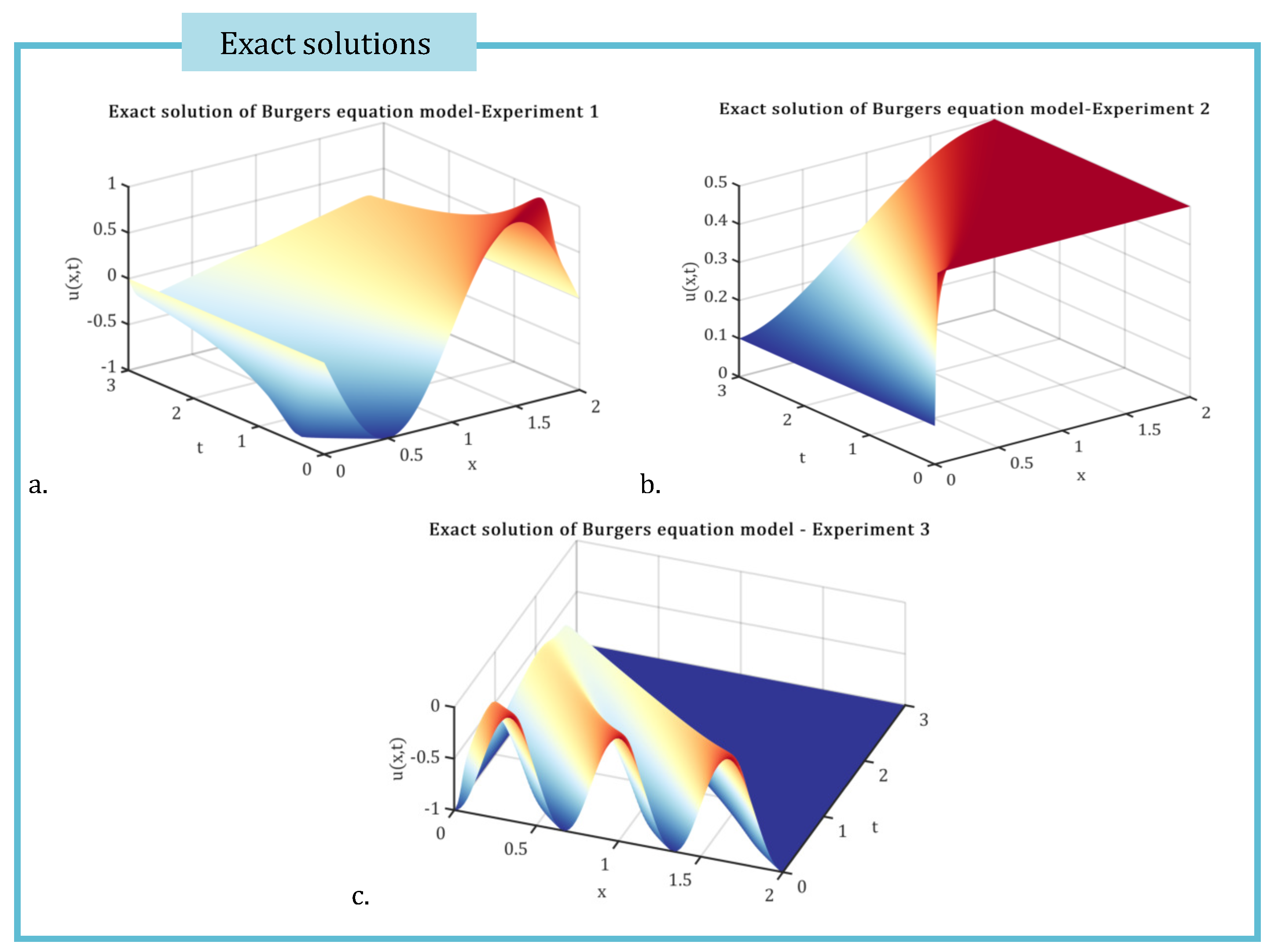
Figure 2.
The objectives of the optimization problem (46) and Pareto front solution obtained by genetic algorithm, for the three experiments, respectively.
Figure 2.
The objectives of the optimization problem (46) and Pareto front solution obtained by genetic algorithm, for the three experiments, respectively.
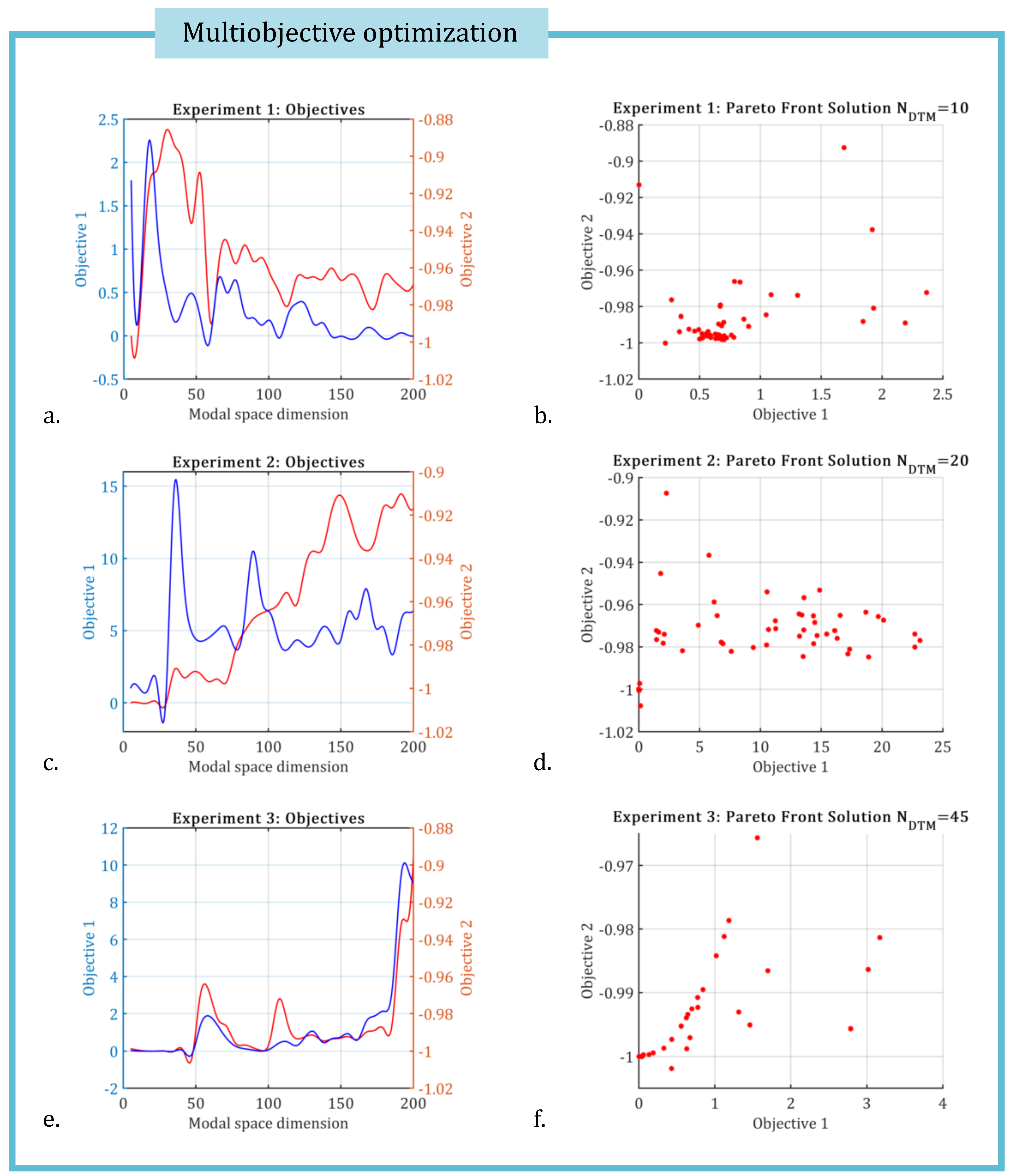
Figure 3.
The running CPU time for KROD in offline phase, for the three experiments, respectively.
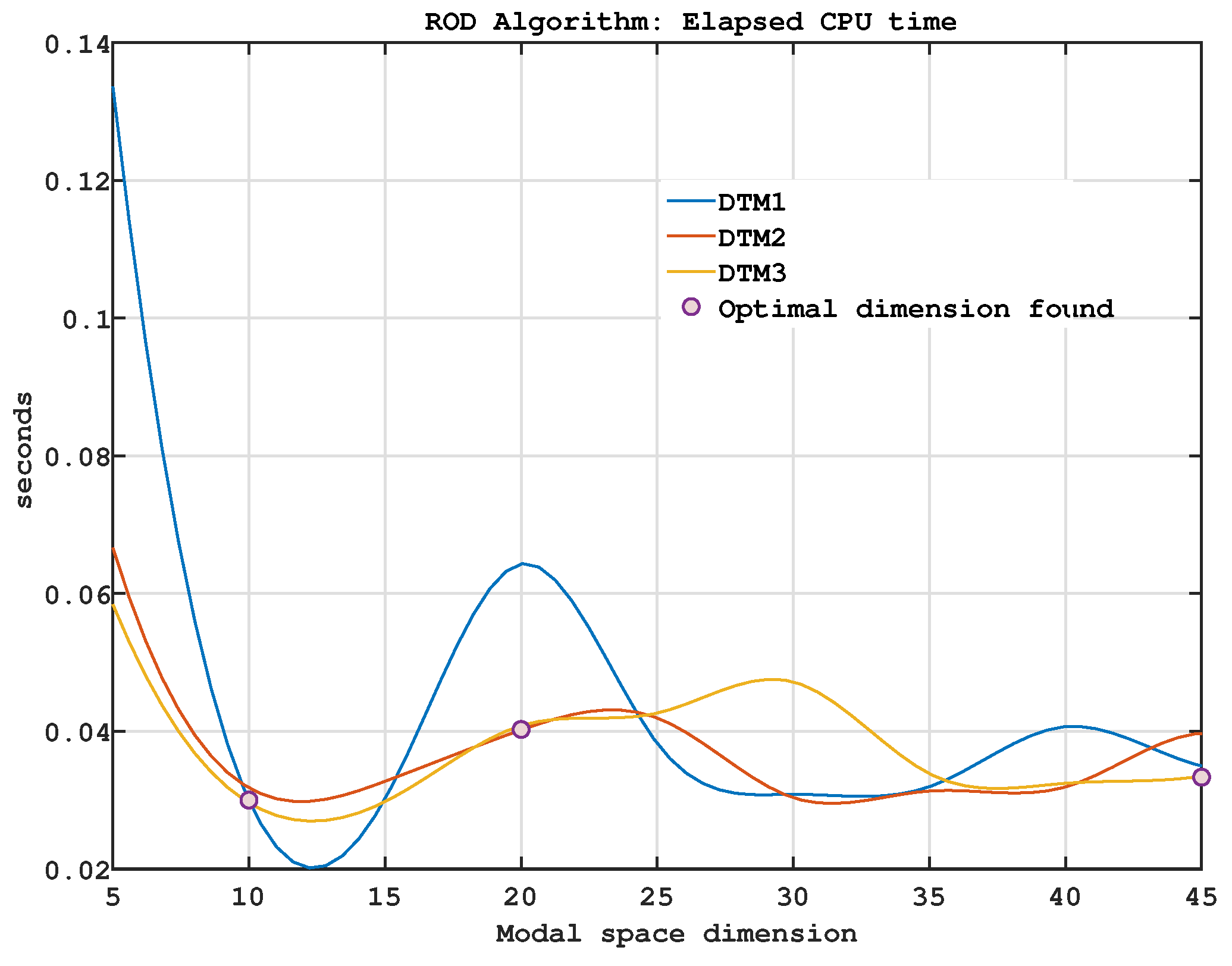
Figure 5.
The two-fold input-output validation is performed for the first two and the last temporal coefficients, as obtained from the simulated responses of the optimal NLARX models in the case of Experiment 1. Performance metrics associated with the deep learning procedure are also are illustrated.
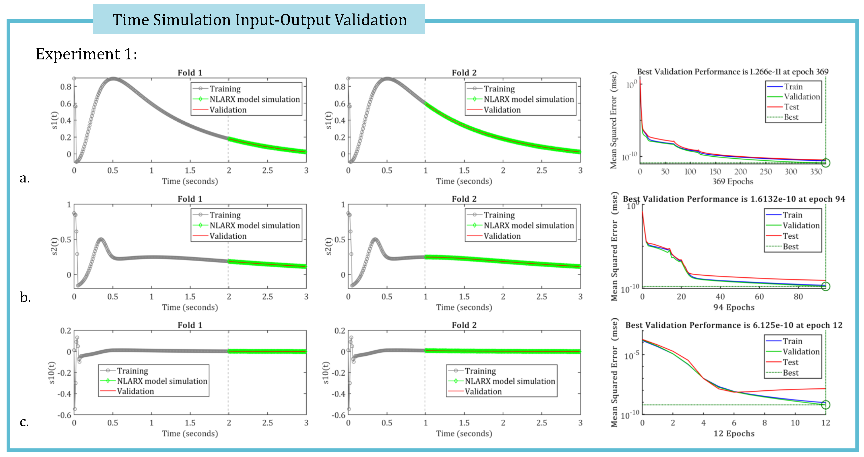
Figure 6.
The two-fold input-output validation is performed for the first two and the last temporal coefficients, as obtained from the simulated responses of the optimal NLARX models in the case of Experiment 2. Performance metrics associated with the deep learning procedure are also are illustrated.
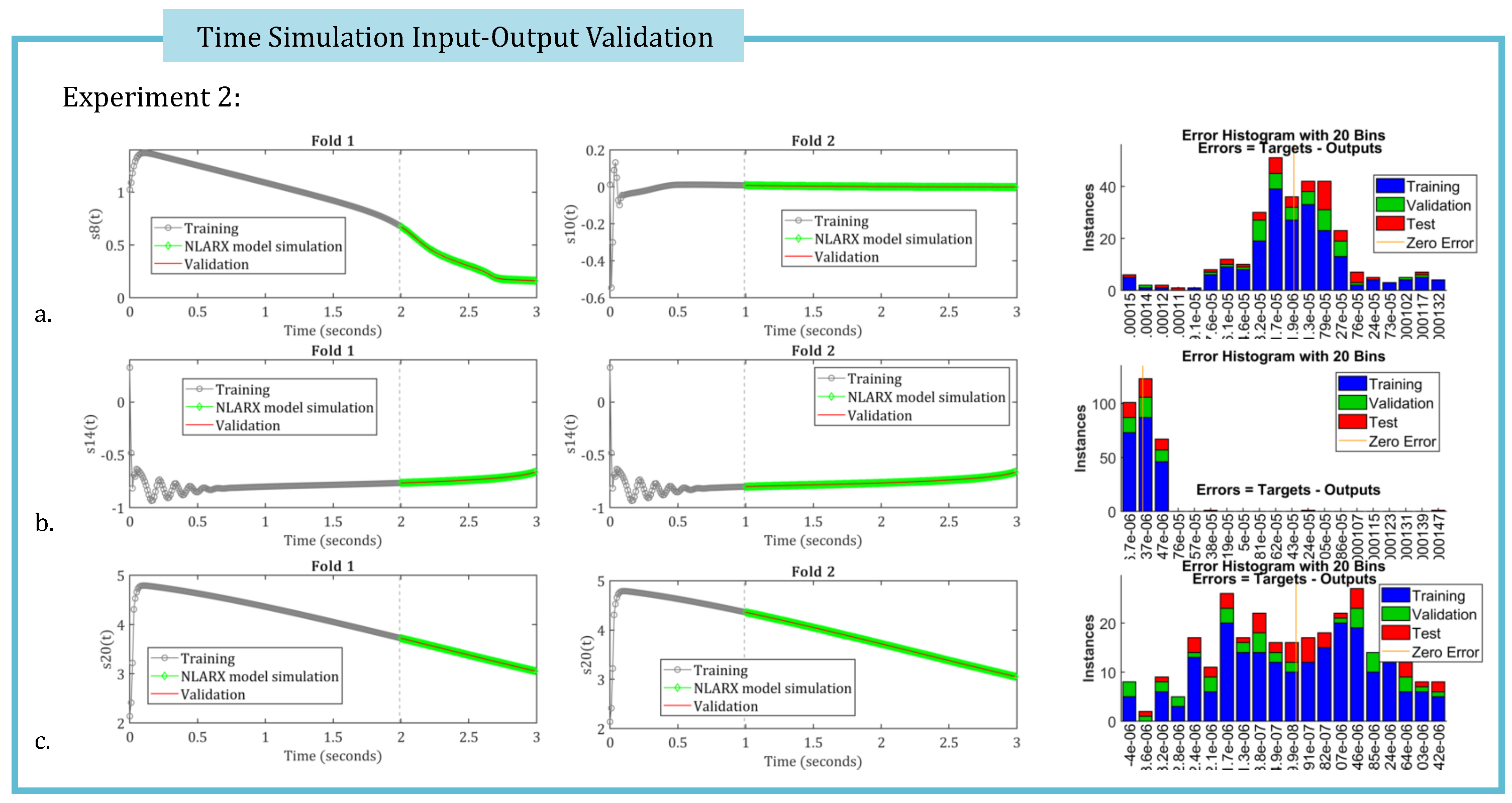
Figure 7.
The two-fold input-output validation is performed for the first two and the last temporal coefficients, as obtained from the simulated responses of the optimal NLARX models in the case of Experiment 3. Performance metrics associated with the deep learning procedure are also are illustrated.
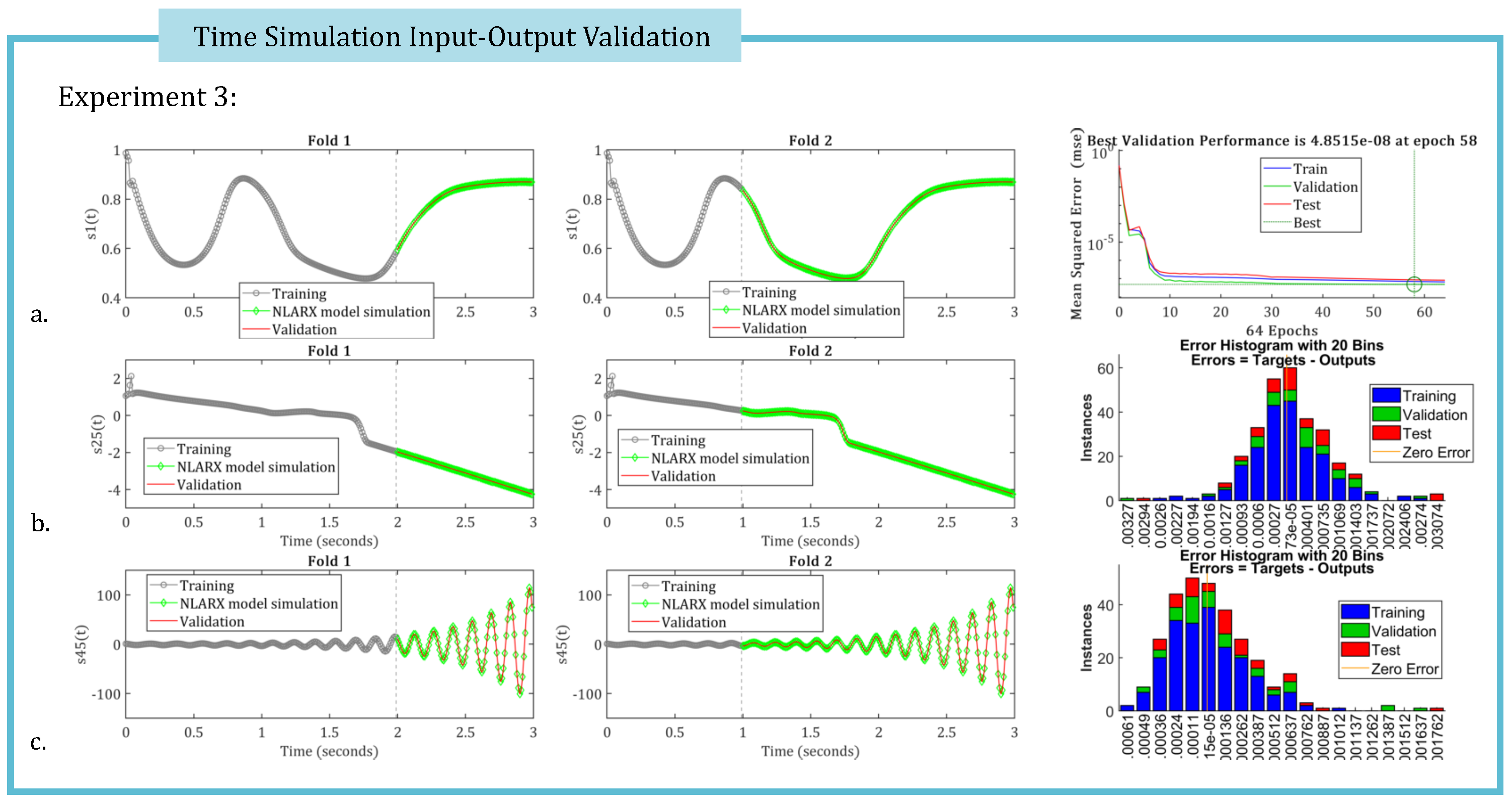
Figure 8.
Time responses of the data-driven twin models for all three experiments are compared against the original data, with the corresponding local errors between the exact solution and the simulated DTM responses also presented.
Figure 8.
Time responses of the data-driven twin models for all three experiments are compared against the original data, with the corresponding local errors between the exact solution and the simulated DTM responses also presented.
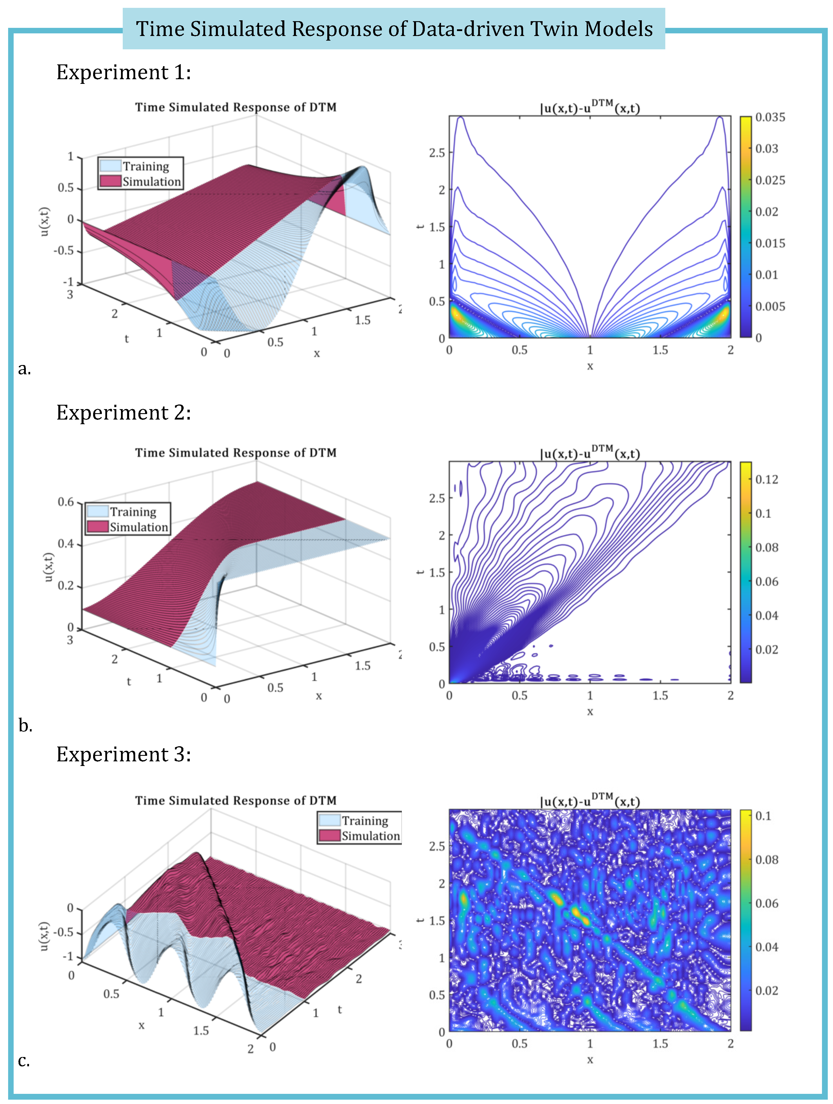
Figure 9.
The running CPU time for the online phase of the algorithm, with respect to the modal space dimension optimized in the case of the three experiments considered.
Figure 9.
The running CPU time for the online phase of the algorithm, with respect to the modal space dimension optimized in the case of the three experiments considered.

Disclaimer/Publisher’s Note: The statements, opinions and data contained in all publications are solely those of the individual author(s) and contributor(s) and not of MDPI and/or the editor(s). MDPI and/or the editor(s) disclaim responsibility for any injury to people or property resulting from any ideas, methods, instructions or products referred to in the content. |
© 2025 by the authors. Licensee MDPI, Basel, Switzerland. This article is an open access article distributed under the terms and conditions of the Creative Commons Attribution (CC BY) license (http://creativecommons.org/licenses/by/4.0/).
Copyright: This open access article is published under a Creative Commons CC BY 4.0 license, which permit the free download, distribution, and reuse, provided that the author and preprint are cited in any reuse.


