
Submitted:
05 June 2025
Posted:
12 June 2025
You are already at the latest version
Abstract
Neural ordinary differential equations (neural ODEs) are a well-established tool for optimizing the parameters of dynamical systems, with applications in image classification, optimal control, and physics-learning. Although dynamical systems of interest often evolve on Lie groups and more general differentiable manifolds, theoretical results on neural ODEs are frequently phrased on $\R^n$. We collect recent results on neural ODEs on manifolds, and present a unifying derivation of various results that serves as a tutorial to extend existing methods to differentiable manifolds. We also extend the results to the recent class of neural ODEs on Lie groups, highlighting a non-trivial extension of manifold neural ODEs that exploits the Lie group structure.
Keywords:
Neural Ordinary Differential Equations
; Differential Geometry
; Lie groups
; Machine Learning
; Optimal Control
1. Introduction
Ordinary differential equations (ODEs) are ubiquitious in the engineering sciences, from modeling and control of simple physical systems like pendulums and mass-spring dampers, or more complicated robotic arms and drones, to the description of high-dimensional spatial discretizations of distributed systems, such as fluid flows, chemical reactions or quantum oscillators. Neural ordinary differential equations (neural ODEs) [1,2] are ODEs parameterized by neural networks. Given a state x, and parameters representing weights and biases of a neural network, a neural ODE reads:
First introduced by [1] as the continuum limit of recurrent neural networks, the number of applications of neural ordinary differential equations quickly exploded beyond simple classification tasks: learning highly nonlinear dynamics of multi-physical systems from sparse data [3,4,5], optimal control of nonlinear systems [6], medical imaging [7] and real-time handling of irregular time-series[8], to name but a few. Discontinuous state-transitions and dynamics [9,10], time-dependent parameters [11], augmented neural ODEs [12] and physics preserving formulations [13,14] present further extensions that increase the expressivity of neural ODEs.
However, these methods are typically phrased for states . For many physical systems of interest, such as robot arms, humanoid robots and drones, the state lives on differentiable manifolds and Lie groups [15,16]. More generally, the manifold hypothesis in machine learning raises the expectation that many high-dimensional data-sets evolve on intrinsically lower-dimensional, albeit more complicated manifolds [17]. Neural ODEs on manifolds [18,19] presented significant steps to address this gap, presenting first optimization methods for neural ODEs on manifolds. Yet, the general tools and approaches available on , such as including running costs, augmented states, time-dependent parameters, control-inputs or discontinuous state-transitions, are rarely addressed in a manifold context. Similar issues persist in a Lie group context, were Neural ODEs on Lie groups [20,21] were formalized.
Our goal is to extend more of the methods for neural ODEs on to arbitrary manifolds, and in particular Lie groups. To this end, we present a systematic approach to the design of neural ODEs on manifolds and Lie groups. Specifically, our contributions are:
- Systematic derivation of neural ODEs on manifolds and Lie groups, highlighting differences and equivalence of various approaches - for an overview, see also Table 1;
- Summarizing the state of the art on manifold and Lie group neural ODEs, by formalizing the notion of extrinsic and intrinsic neural ODEs;
- A tutorial-like introduction, to assist the reader in implementing various neural ODE methods on manifolds and Lie groups, presenting coordinate expressions alongside geometric notation.
The remainder of the article is organized as follows. A brief state-of-the-art on neural ODEs concludes this introduction. Section 2 provides background on differentiable manifolds, Lie groups, and the coordinate-free adjoint method. Section 3 describes neural ODEs on manifolds, and derives parameter updates via the adjoint method for various common architectures and cost-functions, including time-dependent parameters, augmented neural ODEs, running costs, and intermediate cost-terms. Section 4 describes neural ODEs on matrix Lie groups, explaining merits of treating Lie groups separately from general differentiable manifolds. Both Section 3 and Section 4 also classify methods into extrinsic and intrinsic approaches. We conclude with a discussion in Section 5, highlighting advantages, disadvantages, challenges and promises of the presented material. The Appendix includes background on Hamiltonian systems, which appear when transforming the adjoint method into a form that is unique to Lie groups.
1.1. Literature review
For a general introduction to neural ODEs, see [25]. Neural ODEs on with fixed parameters were first introduced by [1], and parameter optimization via the adjoint method allowed for intermittent and final cost terms on each trajectory. The generalized adjoint method [2] also allows for running cost terms. Memory-efficient checkpointing is introduced in [26] to address stability issues of adjoint methods. Augmented neural ODEs [12] introduced augmented state-spaces to allow neural ODEs to express arbitrary diffeomorphisms. Time-varying parameters were introduced by [11], with similar benefits to augmented neural ODEs. Neural ODEs with discrete transitions were formulated in [9,10], with [9] also learning event-triggered transitions common in engineering application. Neural controlled differential equations (CDEs) were introduced in [27] for handling irregular time-series, and parameter updates reapply the adjoint method [1]. Neural stochastic differential equations (SDEs) were introduced in [28], relying on a stochastic variant of the adjoint method for the parameter update. The previously mentioned literature phrases dynamics of neural ODEs on .
Neural ODEs on manifolds were first introduced by [22], including an adjoint method on manifolds for final cost terms, and application to continuous normalizing flows on Riemannian manifolds, but embedding manifolds into . Neural ODEs on Riemannian manifolds are expressed in local exponential charts in [18], avoiding embedding into , and considering final cost terms in the optimization. Charts for unknown, nontrivial latent manifolds, and dynamics in local charts, are learned from high-dimensional data in [29], including also discretized solutions to partial differential equations. Parameterized equivariant Neural ODEs on manifolds are constructed in [23], also commenting on state augmentation to express arbitrary (equivariant) flows on manifolds.
Neural ODEs on Lie groups were first introduced in [30] on the Lie group , to learn the port-Hamiltonian dynamics of a drone from experiment, expressing group elements on an embedding , and the approach was formalized to port-Hamiltonian systems on arbitrary matrix Lie groups in [20], embedding matrices in .
Neural ODEs on were phrased in local exponential charts in [24] to optimize a controller for a rigid body, using a chart-based adjoint method in local expential charts. An alternative, Lie algebra based adjoint method on general Lie groups was introduced in [21], foregoing Lie group specific numerical issues of applying the adjoint method in local charts.
1.2. Notation
For a complete introduction to differential geometry see e.g, [31], and for Lie group theory see [32].
Calligraphic letters denote smooth manifolds. For conceptual clarity, the reader may think of these manifolds as embedded in a high dimensional , e.g., . The set contains smooth functions between and , and we define :.
The tangent space at is and the cotangent space is . The tangent bundle of is , and the cotangent bundle of is . Then denotes the set of vector fields over , and denotes the set of k forms, where are co-vector fields, and are smooth functions . The exterior derivative is denoted as . For functions , with , , we denote by the partial differential at . Curves are denoted as , and their tangent vectors are denoted as .
A Lie group is denoted by G, its elements by . The group identity is , and I denotes the identity matrix. The Lie algebra of G is , and its dual is . Letters denote vectors in the Lie algebra, while letters denote vectors in .
In coordinate expressions lower indices are covariant and upper indices are contravariant components of tensors. For example, for a -tensor M, the components are covariant, and for non-degenerate M, the components of its inverse are , which are contravariant. We use the Einstein summation convention , i.e., the product of variables with repeated lower and upper indices implies a sum.
Denoting W a topological space, D the Borel -algebra and a probability measure, then the tuple denotes a probability space. Given a vector space L and a random variable , then the expectation of C w.r.t. is .
2. Background
2.1. Smooth Manifolds
Given an n-dimensional manifold, with an open set and a homeomorphism, we call a chart and we denote the coordinates of as
Smooth manifolds admit charts and with smooth transition maps defined on the intersection , and a collection of charts with smooth transition maps is called a (smooth) atlas. A vector field associates to any point a vector in . It defines a dynamic system
and we denote the solution of (3) by the flow operator
For a real valued function , its differential is the covector field
Given additionally a smooth manifold and a smooth map , with and appropriate charts of and , respectively. Then the pullback of V via is
With a Riemannian metric M (i.e., a symmetric, non-degenerate (0,2) tensor field) on , the gradient of V is a uniquely defined vector field given by
When , we assume that M is the Euclidean metric, and pick coordinates such that the components of the gradient and differential are the same. Finally, we define the Lie derivative of 1-forms, which differentiates along a vector field and returns :
2.2. Lie groups
Lie groups are smooth manifolds with a compatible group structure. We consider real matrix lie groups , i.e., subgroups of the general linear group
For the left and right translations by h are, respectively, the matrix multiplications
The Lie algebra of G is the vector space , with the Lie algebra of .
Define a basis with , and Define the (invertible, linear) map as1
The dual of is denoted , and given the map we call its dual. For the small adjoint is a bilinear map, and the large Adjoint is the linear map is a linear map
In the remainder of the article, we exclusively use the adjoint representation , written without a tilde in the subscript A, and Adjoint representation which are obtained as
Its inverse is a given by the matrix logarithm, and it is well-defined on a subset [Chapter 2.3 [32]:
Often, these infinite sums in (17) and (18) can further be reduced to a finite sums in m terms, by use of the Cayley-Hamilton Theorem [34]. A chart on G that assigns zero coordinates to can be defined using (18) and (12)
The chart is called an exponential chart, and a collection of exponential charts that cover the manifold is called an exponential atlas.
The differential of a function is the co-vector field (see also Equation (5)). For any given we further transform the co-vector to a left-trivialized differential, which collects the components of the gradient expressed in :
For a derivation of this coordinate expression, see [Sec. 3 [21].
2.3. Gradient over a flow
We will be interested in computing the gradient of functions with respect to the initial state of a flow. The adjoint sensitivity equations are a set of differential equations that achieve this. In the following, we show a derivation of the adjoint sensitivity on manifolds [21]. Given a function , a vector field , the associated flow , and a final time , the goal of the adjoint sensitvity method on manifolds is to compute the gradient
In the adjoint method we define a co-state , which represents the differential of with respect to . The adjoint sensitivity method describes its dynamics, which are integrated backwards in time from the known final condition , see also Figure 1. The adjoint sensitivity method is stated in Theorem 1.
Theorem 1
(Adjoint sensitivity on manifolds). The gradient of a function is
where is the co-state. In a local chart of with induced coordinates on , and satisfy the dynamics
Proof.
Define the co-state as
A derivation of the dynamics governing constitutes the remainder of this proof. By definition of and the Lie derivative (8), we have that :
If we further treat as a 1-form (denoted as , by an abuse of notation), we obtain:
The components satisfy the partial differential equation
Impose that (this defines the 1-form along ), then
Expanding the final condition in local coordinates (see Equation (5)) gives
□
A fact that will become useful in Section 4, is that the equations (24) and () have a Hamiltonian form. Define the control Hamiltonian as
Then Equation (24) and Equation (), respectively, of Theorem 1 follow as the Hamiltonian equations on :
For background on Hamilton’s equations, see also Appendix A.1.
3. Neural ODEs on Manifolds
A neural ODE on a manifold is an NN-parameterized vector field in – or including time dependence, it is an NN-parameterized vector field in , with t in the slot and . Given parameters , we denote this parameterized vector field as . This results in the dynamic system
The key idea of neural ODEs is to tackle various flow approximation tasks, by optimising the parameters with respect to a to-be-specified optimization problem. Denote a finite time horizon T and intermittent times . Denote a general trajectory cost by
with intermittent and final cost term F, and running cost r. Indicating a probability space , we define the total cost as
The minimization problem takes the form
Note that (39) is not subject to any dynamic constraint - the flow already appears explicitly in the cost .
Normally, the optimization problem is solved by means of a stochastic gradient descent optimization algorithm [35]. In this, a batch of N initial conditions is sampled from the probability distribution corresponding to the probability measure . Writing , the parameter gradient is approximated as
In this section, we show how to optimize the parameters for various choices of neural ODEs and cost functions, with (37) the most general case of a cost, and highlight similarities in the various derivations. In the following, the gradient is computed via the adjoint method on manifolds, for various scenarios. The advantage of the adjoint method over e.g., automatic differentiation of / back-propagation through an ODE solver, is that it has a constant memory efficiency with respect to the network depth T.
3.1. Constant parameters, running and final cost
Here we consider neural ODEs of the form (36), with constant parameters , and cost functions of the form
with a final cost term F and a running cost term r. This generalizes [1,2] to manifolds. Compared to existing manifold methods for neural ODES [18,19], the running cost is new.
The parameter gradient’s components are then computed by Theorem 2 (see also [21]):
Theorem 2
(Generalized Adjoint Method on Manifolds). Given the dynamics (36) and the cost (41), the parameter gradient’s components are computed by
where the state and co-state satisfy, in a local chart with ,
Proof.
Define the augmented state space as , to include the original state , parameters , accumulated running cost and time in the augmented state . In addition, define the augmented dynamics as
This is an autonomous system with final state . Next, define the cost on the augmented space:
Then Equation (41) can be rewritten as the evaluation of a terminal cost :
By Theorem 1, the gradient is given by
and by Equation (), the componentents of satisfy
Split the co-state into , then their components’ dynamics are:
In summary, the above proof dependeds on identifying a suitable augmented manifold , with the goal that augmented dynamics are autonomous, and that the cost-function on the augmented manifold rephrases the cost (41) as a final cost , which allows to apply Theorem 1, and express any gradients of the original cost. In later sections (Sec. Section 3.2), this process will be the main technical tool for generalizations of Theorem (2). The next sections describe common special cases of (36) and Theorem 2.
3.1.1. Vanilla neural ODEs and extrinsic neural ODEs on manifolds
The case of neural ODEs on (e.g., [1,2]) is obtained by setting . In this case, one global chart can be used to represent all quantities.
This overlaps with extrinsic neural ODEs on manifolds (described, for instance, in [22]), which optimize the neural ODE on an embedding space . We denote this embedding as , let and . Optimizing the neural ODE on requires extending the dynamics to a vector field , such that
The dynamics are then used in Theorem 2, and also the costate lives in .
As shown in [22], the resulting parameter gradients are equivalent to those resulting from an application in local charts, as long as it can be guaranteed that the integral curves of remain within , i.e., are geometrically preserving.
A strong upside of an extrinsic formulation is that existing neural ODE packages (e.g., [36]) can be applied directly. Possible downsides of extrinsic neural ODEs are that finding may not be immediate, a geometrically preserving integration has to be guaranteed separately, and that N is larger than the intrinsic dimension , leading to computational overhead.
3.1.2. Intrinsic neural ODEs on manifolds
The intrinsic case of neural ODEs on manifolds [18] is described by integrating the dynamics in local charts. Given a chart-transition from a chart to a chart chart transitions of the state and costate components ( and , respectively) are given by
with . The advantage of intrinsic neural ODEs on manifolds over extrinsic neural ODEs on manifolds is that the dimension of the resulting equations is as low as possible, for the given manifold. A disadvantage lies in having to determine charts, and chart-switching procedures. In available state-of-the-art packages for neural ODEs, these are phrased as discontinuous dynamics with state transitions . For details on chart-switching methods see [18,21,29].
3.2. Extensions
The proof of Theorem 2 depended on identifying a suitable augmented manifold , autonomous augmented dynamics and augmented cost-function that rephrases the cost (41) as a final cost , to apply Theorem 1. This approach generalizes to various other scenarios, including different cost-terms, augmented neural ODEs on manifolds and time-dependent parameters, presented in the following.
3.2.1. Nonlinear and intermittent cost terms
We consider here the case of neural ODEs on manifolds of the form (36) with cost (37). For the final and intermittent cost term we denote by the differential w.r.t. the k-th slot, and denote as a subscript to avoid confusion. The components of will be denoted . In this case, the parameter gradient is determined by repeated application of Theorem 2:
Theorem 3
(Generalized Adjoint Method on Manifolds). Given the dynamics (36) and the cost (37), the parameter gradient’s components are computed by
where the state satisfies (43) and the co-state satisfies dynamics with discrete updates at times given by
with the instance after a discrete update at time (recall that co-state dynamics are integrated backwards, so ), and the instance before.
Proof.
We introduce an augmented manifold , to include N copies of the original state , parameters , accumulated running cost and time in the augmented state . Let
and define the augmented dynamics as
This is an autonomous system with final state
Next, define the cost on the augmented space:
Then Equation (37) can be rewritten as the evaluation of a terminal cost :
Apply Equation (), and split the co-state into , then their components’ dynamics are:
We excluded the dynamics of , which does not appear in any of the other equations, and the constant . Finally, define the cumulative co-state
Its dynamics at are given by the sum of (65) to (), letting :
with discrete jumps (58) accounting for the final conditions of , and the dynamics () can be rewritten as
Integrating this from to recovers Equation (57). □
Cost terms of this form are interesting for optimiziation of e.g., periodic orbits [37] or trajectories on manifolds, where conditions at multiple checkpoints may appear in the cost.
3.2.2. Augmented neural ODEs on manifolds and time-dependent parameters
With state , augmented state (not to be confused with ), and parameterized , augmented neural ODEs on manifolds are neural ODEs on the manifold of the form
Time t is not included explicitly in these dynamics, since it can be included in . This case also includes the scenario of time-dependent parameters as part of . As the trajectory cost, we take a final cost
Theorem 4
Proof.
Define the augmented state space as , to include the states and parameters in the augmented state . In addition, define the augmented dynamics as
This is an autonomous system with final state . Next, define the cost on the augmented space:
Then Equation (41) can be rewritten as the evaluation of a terminal cost . The gradient is given by an application of Equation (). Split the co-state into , then their components’ dynamics are:
Since also depends on , the total gradient of the cost w.r.t. is given by
This recovers Equation (75). □
A further degenerate application of Theorem 4 is obtained by removing x. Then both dynamics and initial condition are parameterized by , allowing joint optimization of parameters and initial condition. This is interesting for joint optimization and numerical continuation, e.g. [37].
4. Neural ODEs on Lie Groups
Just as a neural ODE on a manifold is an NN-parameterized vector field in (or, including time, ), a neural ODE on a Lie group can be seen as a parameterized vector field in (or , respectively). Similarly to Equation (36), this results in a dynamic system
Yet, Lie groups offers more structure than manifolds: the Lie algebra provides a canonical space to represent tangent vectors, and its dual provides a canonical space to represent the co-state. Similarly, canonical (exponential) charts offer structure for integrating dynamic systems [38]. Frequently, dynamics on a Lie group induced dynamics on a manifold : by means of an action
evolutions induce evolutions on . This makes neural ODEs on Lie groups interesting in their own right.
In this section, we describe optimizing (39) for the cost
with a final cost term F and a running cost term r. We highlight the extrinsic approach, and two intrinsic approaches, where one of the latter is peculiar to Lie groups.
4.1. Extrinsic neural ODEs on Lie groups
The extrinsic formulation of neural ODEs on Lie groups was first introduced by [20], and applies ideas of [19] (see also Section 3.1.1). Given , this formulation treats the dynamic system (84) as a dynamic system on . Denote an invertible map that stacks the components of an input matrix matrix into a component vector2 and let be a projection onto . Further denote and . A lift can then be defined as
As was the case for extrinsic neural ODEs on manifolds, the cost-gradient resulting from this optimization is well-defined and equivalent to any intrinsically defined procedure. However, dimension of the vectorization can be significantly larger than the intrinsic dimension of the Lie group.
4.2. Intrinsic neural ODEs on Lie groups
Theorem 2 directly applies to optimization of neural ODEs on Lie groups, given the local exponential charts (19), () on G. This does not make full use of the available structure on Lie groups. Frequently, dynamical systems are of a left-invariant form (88) or a right-invariant form ()
Denoting the derivative of the exponential map (see [21] for details). Then the chart-representatives in a local exponential chart are
Application of Theorem 2 then requires computing or . But this leads to significant computational overhead due differentiation of the terms (see [21]). Instead of applying Theorem 2, i.e., expressing dynamics in local charts, the dynamics can also be expressed at the Lie algebra . Theorem has a Hamiltonian form, which can be directly transformed into Hamiltonian equations on a Lie group (see also Appendix A.1). Applying this reasoning to Theorem 2, we arrive at the following form, which foregoes differentiating :
Theorem 5
(Left Generalized Adjoint Method on Matrix Lie Groups). Given are the dynamics (88) and the cost (86), or the dynamics () with . Then the parameter gradient of the cost is given by the integral equation
where the state and co-state are the solutions of the system of equations
Proof.
This is proven in two steps. First, define the time-and-parameter-dependent control-Hamiltonian as
The equations for the state- and co-state dynamics (43) and (), respectively, of Theorem 2 follow as the Hamiltonian equations on :
And the integral equation (42) reads
Second, rewrite the control Hamiltonian (95) on a Lie group G, i.e., . By substituting (see also Equation (A6)), this induces
Finally Hamilton’s equations (96), () are rewritten in their form on a matrix Lie group by means of (A7), (), which recovers equations (93) and ():
To find the final condition for , use that :
□
Similar equations also hold on abstract (non-matrix) Lie groups, see [21]. Compared to the extrinsic method of Section 4.1, Theorem 5 has the advantage that the dimension of the co-state is as low as possible. Compared to the chart-based approach on Lie groups, Theorem 5 foregoes differentiating through the terms , avoiding overhead. Compared to a chart-based approach on manifolds, also the choice of charts is canonical on Lie groups. Although the Lie-group approach foregoes many of the pitfalls of intrinsic neural ODEs on manifolds, implementation in existing neural ODE packages is currently cumbersome: the adjoint-sensitivity equations () have a non-standard form, requiring an adapted dynamics of the co-state , but these equations are rarely intended for modification, in existing packages. Packages for geometry-preserving integrators on Lie groups, such as [38] are also not readily available for arbitrary Lie groups.
4.3. Extensions
The proof of Theorem 5 relied on finding a control-Hamiltonian formulation for Theorem 2. This approach generalizes to methods in Section 3.2, which rely on the use of Theorem 1. That is because Theorem 1 itself has a Hamiltonian form ([19,21]).
5. Discussion
We discuss advantages and disadvantages of the main flavors of the presented formulations for manifold neural ODEs, expanding on the previous sections. We focus on extrinsic (embedding dynamics in ) and intrinsic (integrating in local charts) formulations. Summarizing prior comments:
- the extrinsic formulation is readily implemented if the low-dimensional manifold and an embedding into are known. This comes at the possible cost of geometric inexactness, and a higher dimension of the co-state and sensitivity equations
- the co-state in the intrinsic formulation has a generally lower dimension, which reduces the dimension of the sensitivity equations. The chart-based formulation also guarantees geometrically exact integration of dynamics. This comes at the mild cost of having to define local charts and chart-transitions.
This dimensionality reduction is unlikely to have a high impact when the manifold is known and low dimensional, e.g., for the sphere or similar manifolds. However, when applying the manifold hypothesis to high-dimensional data, there might be non-trivial latent manifolds for which the embedding is not immediate, and where the latent manifold is of a much lower dimension than the embedding data-manifold. Then the intrinsic method becomes difficult to avoid. If geometric exactness of the integration is desired, local charts need to be defined also for the extrinsic approach, in which case the intrinsic approach may offer further advantages.
In order to derive neural ODEs on Lie groups, three approaches were possible: the extrinsic and intrinsic formulations on manifolds directly carry over to matrix Lie groups, embedding in or using local exponential charts, respectively. A third option a novel intrinsic method for neural ODEs on matrix Lie groups, which made full use of the Lie group structure by phrasing dynamics on (as is more common on Lie groups), and the co-state on , avoiding difficulties of the chart-based formalism in differentiating extra terms.
Summarizing prior comments on advantages and disadvantages of these flavors:
- the extrinsic formulation on matrix Lie groups can come at much higher cost than that on manifolds, since the intrinsic dimension of G can be much lower than , and a higher dimension of the co-state and sensitivity equations. Geometrically exact integration procedures are more readily available for matrix Lie groups, integrating in local exponential charts.
- the chart-based formulation on matrix Lie groups struggles when are not naturally phrased in local charts. This is common, dynamics are often more naturally phrased on . This was alleviated by an algebra-based formulation on matrix Lie groups. Both are intrinsic approaches, that feature a co-state dynamics that are as low as posssible. However, the algebra-based approach still misses readily available software implementation.
The authors believe that the algebra-based formulation is more convenient, in principle, and consider software implementations of the algebra-based approach as possible future work.
In summary, we presented a unified, geometric approach to extend various methods for neural ODEs on to neural ODEs on manifolds and Lie groups. Optimization of neural ODEs on manifolds was based on the adjoint method on manifolds. Given a novel cost-function C and neural ODE architecture f, the strategy to present the results in a unified fashion was to identify a suitable augmented manifold , augmented dynamics , and cost such that the original cost-function can be rephrased as . To further derive optimization of intrinsic neural ODEs on Lie groups was based on finding a Hamiltonian formulation of the adjoint method on manifolds, and to subsequently transformed them into the Hamiltonian equations on a matrix Lie group.
Author Contributions
Conceptualization, Y.P.W.; methodology, Y.P.W.; software, Y.P.W.; validation, Y.P.W.; formal analysis, Y.P.W.; investigation, Y.P.W.; resources, S.S.; data curation, Y.P.W.; writing—original draft preparation, Y.P.W.; writing—review and editing, Y.P.W., F.C., S.S.; visualization, Y.P.W.; supervision, F.C., S.S.; project administration, S.S.; funding acquisition, S.S. All authors have read and agreed to the published version of the manuscript.
Data Availability Statement
Not applicable.
Conflicts of Interest
The authors declare no conflicts of interest. The funders had no role in the design of the study; in the collection, analyses, or interpretation of data; in the writing of the manuscript; or in the decision to publish the results.
Appendix A. Additional Material
Appendix A.1. Hamiltonian dynamics on Lie groups
We briefly review Hamiltonian systems on manifolds and matrix Lie groups (see also [21]).
Given a manifold with coordinate maps and in the basis on , we define the symplectic form as
Let , then a Hamiltonian implicitly defines a unique vector field by
In coordinates, has the components
On a Lie group G, the group structure allows the identification . E.g., using the pull back of left-translation map , and , to define as
Then the left Hamiltonian is defined in terms of as
References
- Chen, R.T.Q.; Rubanova, Y.; Bettencourt, J.; Duvenaud, D. Neural Ordinary Differential Equations. CoRR, 1806. [Google Scholar]
- Massaroli, S.; Poli, M.; Park, J.; Yamashita, A.; Asama, H. Dissecting neural ODEs. Advances in Neural Information Processing Systems, 2002. [Google Scholar]
- Zakwan, M.; Natale, L.D.; Svetozarevic, B.; Heer, P.; Jones, C.; Trecate, G.F. Physically Consistent Neural ODEs for Learning Multi-Physics Systems*. IFAC-PapersOnLine 2023, 56, 5855–5860. [Google Scholar] [CrossRef]
- Sholokhov, A.; Liu, Y.; Mansour, H.; Nabi, S. Physics-informed neural ODE (PINODE): embedding physics into models using collocation points. Scientific Reports 2023 13:1 2023, 13, 1–13. [Google Scholar] [CrossRef] [PubMed]
- Ghanem, P.; Demirkaya, A.; Imbiriba, T.; Ramezani, A.; Danziger, Z.; Erdogmus, D. Learning Physics Informed Neural ODEs With Partial Measurements. AAAI-25, arXiv:cs.LG/2412.08681].
- Massaroli, S.; Poli, M.; Califano, F.; Park, J.; Yamashita, A.; Asama, H. Optimal Energy Shaping via Neural Approximators. SIAM Journal on Applied Dynamical Systems 2022, 21, 2126–2147. [Google Scholar] [CrossRef]
- Niu, H.; Zhou, Y.; Yan, X.; Wu, J.; Shen, Y.; Yi, Z.; Hu, J. On the applications of neural ordinary differential equations in medical image analysis. Artificial Intelligence Review 2024, 57, 1–32. [Google Scholar] [CrossRef]
- Oh, Y.; Kam, S.; Lee, J.; Lim, D.Y.; Kim, S.; Bui, A.A.T. Comprehensive Review of Neural Differential Equations for Time Series Analysis 2025.
- Poli, M.; Massaroli, S.; Yamashita, S.A.J.O.N.L.S.C.N.A.L.A.; Asama, H.; Garg, A. Neural Hybrid Automata: Learning Dynamics with Multiple Modes and Stochastic Transitions 2021.
- Chen, R.T.Q.; Amos, B.; Nickel, M. Learning Neural Event Functions for Ordinary Differential Equations 2021.
- Davis, J.Q.; Choromanski, K.; Varley, J.; Lee, H.; Slotine, J.J.; Likhosterov, V.; Weller, A.; Makadia, A.; Sindhwani, V. Time Dependence in Non-Autonomous Neural ODEs 2020. arXiv:cs.LG/2005.01906].
- Dupont, E.; Doucet, A.; Teh, Y.W. Augmented Neural ODEs 2019. arXiv:stat.ML/1904.01681].
- Chu, H.; Miyatake, Y.; Cui, W.; Wei, S.; Furihata, D. Structure-Preserving Physics-Informed Neural Networks With Energy or Lyapunov Structure, 2024, [arXiv:cs.LG/2401.04986]. arXiv:cs.LG/2401.04986].
- Kütük, M.; Yücel, H. Energy dissipation preserving physics informed neural network for Allen–Cahn equations. Journal of Computational Science 2025, 87, 102577. [Google Scholar] [CrossRef]
- Bullo, F.; Murray, R.M. Tracking for fully actuated mechanical systems: a geometric framework. Automatica 1999, 35, 17–34. [Google Scholar] [CrossRef]
- Marsden, J.E.; Ratiu, T.S. Introduction to Mechanics and Symmetry; Vol. 17, Springer New York, 1999. [CrossRef]
- Whiteley, N.; Gray, A.; Rubin-Delanchy, P. Statistical exploration of the Manifold Hypothesis 2025. arXiv:stat.ME/2208.11665].
- Lou, A.; Lim, D.; Katsman, I.; Huang, L.; Jiang, Q.; Lim, S.N.; De Sa, C. Neural Manifold Ordinary Differential Equations. Advances in Neural Information Processing Systems, 2006. [Google Scholar]
- Falorsi, L.; Davidson, T.R.; Berkeley, A.U.C.; Forré, P.; Mar, M.L. Reparameterizing Distributions on Lie Groups 2019. 89, arXiv:1903.02958v1].
- Duong, T.; Altawaitan, A.; Stanley, J.; Atanasov, N. Port-Hamiltonian Neural ODE Networks on Lie Groups for Robot Dynamics Learning and Control. IEEE Transactions on Robotics 2024, 40, 3695–3715. [Google Scholar] [CrossRef]
- Wotte, Y.P.; Califano, F.; Stramigioli, S. Optimal potential shaping on SE(3) via neural ordinary differential equations on Lie groups. The International Journal of Robotics Research 2024, 43, 2221–2244. [Google Scholar] [CrossRef]
- Falorsi, L.; Forré, P. Neural Ordinary Differential Equations on Manifolds, 2020, [2006. 0 6663.
- Andersdotter, E.; Persson, D.; Ohlsson, F. Equivariant Manifold Neural ODEs and Differential Invariants 2024.
- Wotte, Y. Optimal Potential Energy Shaping on SE(3) via Neural Approximators. University of Twente Archive 2021. [Google Scholar]
- Pau, B.S. An introduction to neural ordinary differential equations 2024.
- Gholami, A.; Keutzer, K.; Biros, G. ANODE: Unconditionally Accurate Memory-Efficient Gradients for Neural ODEs 2019. arXiv:cs.LG/1902.10298].
- Kidger, P.; Morrill, J.; Foster, J.; Lyons, T.J. Neural Controlled Differential Equations for Irregular Time Series. CoRR, 2005. [Google Scholar]
- Li, X.; Wong, T.K.L.; Chen, R.T.Q.; Duvenaud, D. Scalable Gradients for Stochastic Differential Equations 2020. arXiv:cs.LG/2001.01328].
- Floryan, D.; Graham, M.D. Data-driven discovery of intrinsic dynamics. Nature Machine Intelligence 2022, 4, 1113–1120. [Google Scholar] [CrossRef]
- Duong, T.; Atanasov, N. Hamiltonian-based Neural ODE Networks on the SE(3) Manifold For Dynamics Learning and Control 2021. [2106.12782v3].
- Isham, C.J. Modern Differential Geometry for Physicists; 1999. [CrossRef]
- Hall, B.C. Lie Groups, Lie Algebras, and Representations: An Elementary Introduction; Graduate Texts in Mathematics (GTM, volume 222), Springer, 2015.
- Solà, J.; Deray, J.; Atchuthan, D. A micro Lie theory for state estimation in robotics, 2021, [arXiv:cs.RO/1812.01537]. arXiv:cs.RO/1812.01537].
- Visser, M.; Stramigioli, S.; Heemskerk, C. Cayley-Hamilton for roboticists. IEEE International Conference on Intelligent Robots and Systems 2006, 1, 4187–4192. [Google Scholar] [CrossRef]
- Robbins, H.; Monro, S. A Stochastic Approximation Method. The Annals of Mathematical Statistics 1951, 22, 400–407. [Google Scholar] [CrossRef]
- Poli, M.; Massaroli, S.; Yamashita, A.; Asama, H.; Park, J. TorchDyn: A Neural Differential Equations Library 2020. [2009.09346].
- Wotte, Y.P.; Dummer, S.; Botteghi, N.; Brune, C.; Stramigioli, S.; Califano, F. Discovering efficient periodic behaviors in mechanical systems via neural approximators. Optimal Control Applications and Methods 2023, 44, 3052–3079. [Google Scholar] [CrossRef]
- Munthe-Kaas, H. High order Runge-Kutta methods on manifolds. Applied Numerical Mathematics 1999, 29, 115–127. [Google Scholar] [CrossRef]
| 1 | Equivalently (e.g, [33]), and are often denoted as operators “hat” and “vee” , respectively. |
| 2 | in canonical coordinates on and , though this choice is not required. |
Figure 1.
(a) The problem of computing the gradient over a flow, highlighting the cotangent spaces and . (b) In the adjoint method we set , whose dynamics are uniquely determined by the property , allowing to find by integrating backwards from .
Figure 1.
(a) The problem of computing the gradient over a flow, highlighting the cotangent spaces and . (b) In the adjoint method we set , whose dynamics are uniquely determined by the property , allowing to find by integrating backwards from .
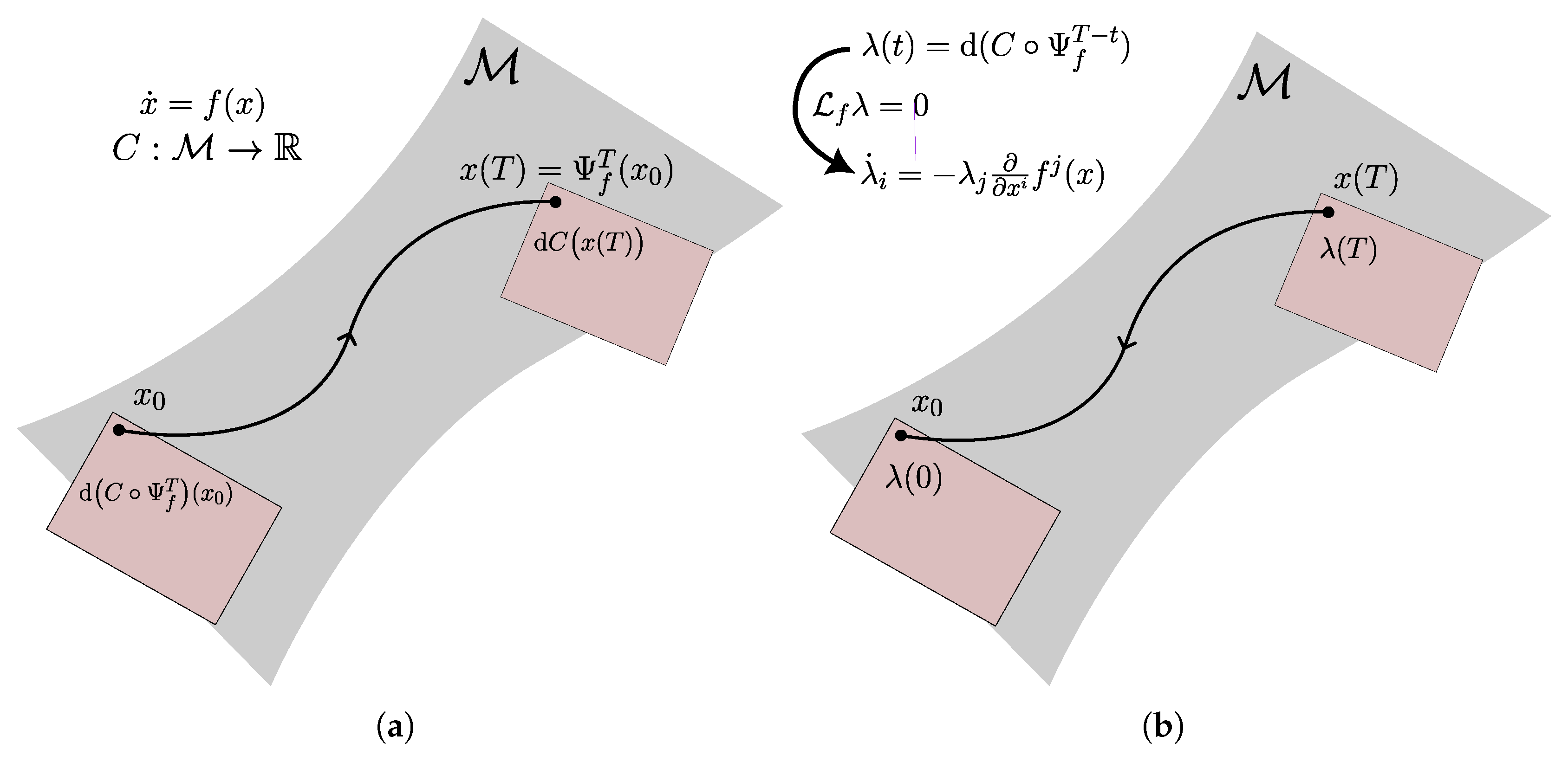

Table 1.
Summary of neural ODEs on manifolds and Lie groups presented in this article
| Name of Neural ODE | Subtype | Trajectory Cost | Subsection | Originally introduced in |
|---|---|---|---|---|
| Neural ODEs on manifolds (Section 3) | Extrinsic | Running and final cost | Section 3.1.1 | Final cost [22], running cost [21] |
| Intrinsic | Running and final cost , intermittent cost | Section 3.1.2 | Final cost [18], running cost [21], intermittent cost (this work) | |
| Augmented, time-dependent parameters | Final cost | Section 3.2.2 | Augmenting to [23], Augmenting to (this work) | |
| Neural ODEs on Lie groups (Section 4) | Extrinsic | Final cost and intermittent cost | Section 4.1 | In [20] |
| Intrinsic, dynamics in local charts | Running and final cost | Section 4.2 | In [21,24] | |
| Intrinsic, dynamics at Lie algebra | Running and final cost | Section 4.2 | In [21] |
1 Tables may have a footer.
Disclaimer/Publisher’s Note: The statements, opinions and data contained in all publications are solely those of the individual author(s) and contributor(s) and not of MDPI and/or the editor(s). MDPI and/or the editor(s) disclaim responsibility for any injury to people or property resulting from any ideas, methods, instructions or products referred to in the content. |
© 2025 by the authors. Licensee MDPI, Basel, Switzerland. This article is an open access article distributed under the terms and conditions of the Creative Commons Attribution (CC BY) license (https://creativecommons.org/licenses/by/4.0/).
Copyright: This open access article is published under a Creative Commons CC BY 4.0 license, which permit the free download, distribution, and reuse, provided that the author and preprint are cited in any reuse.


