Submitted:
01 May 2025
Posted:
02 May 2025
You are already at the latest version
Abstract
This paper addresses the problem of synthesizing four-link initial kinematic chains with rotational pairs for designing flat lever mechanisms with specified motion laws of the input and output links. The proposed method formulates the synthesis problem as an optimization process involving three moving planes Q, Q1 and Q2. Each plane performs distinct motions: Q is fixed, Q1 rotates around a point A, and Q2 undergoes plane-parallel motion. The goal is to determine the optimal position of point A∈Q, B∈Q1 and C∈Q2 such that the distance between points B and C remains nearly constant across multiple configurations. The synthesis problem is reduced to a sequence of linear systems of equations corresponding to three iterative minimization stages: Determining the fixed-point A and the radius R for given points B and C; Determining the point B and radius R for a given point C; Determining the point C and radius R for a given point B. The algorithm uses a hierarchical optimization process to iteratively refine the positions of A, B, and C until convergence is achieved. The convergence criteria are defined by the small changes in the positions of these points and the radius R between iterations. The proposed method avoids solving a highly nonlinear system directly by decomposing the problem into simpler linear systems, ensuring computational efficiency and robustness. The solution provides the desired positions of the points, forming an open kinematic chain ABCD with three degrees of freedom. The approach is applicable to the synthesis of complex planar mechanisms with unrestricted parameters, making it a valuable tool for mechanism design.
Keywords:
kinematic synthesis
; initial kinematic chain
; approximate kinematic geometry
; objective function minimization
; system of linear equations.
1. Introduction
This paper explores the challenges of kinematic synthesis for four-link initial kinematic chains, which are fundamental in the design of planar (flat) lever mechanisms. Such synthesis is especially important in developing high-class mechanisms [1,2,3], where specific motion laws are imposed on both input and output links [4]. The core of the synthesis problem lies in defining a plane-parallel motion of two rigid bodies (or their planar cross-sections) with respect to a third, fixed body [5,6]. The approach is grounded in the theory of approximate kinematic geometry, which allows for practical realization of mechanisms based on discrete positional data. The synthesis of four-link initial kinematic chains with rotational pairs is a fundamental problem in the design of planar lever mechanisms, especially high-class mechanisms with prescribed laws of motion for input and output links. This problem arises frequently in the design of machinery where precise coordination of moving components is required, such as robotic manipulators, mechanical linkages [7,8], and automated systems. The challenge lies in finding appropriate geometric configurations that satisfy desired motion criteria while ensuring kinematic compatibility and smooth operation [9,10]. Traditional methods for mechanism synthesis often rely on graphical or analytical approaches, which can be cumbersome and limited in their application. As mechanisms become more complex, particularly those involving rotational and translational pairs [11], the design process requires more robust mathematical tools. Recent advancements in computational techniques have enabled the development of more efficient and accurate methods for solving synthesis problems [12,13,14], particularly when formulating them as optimization problems. In this work, we focus on the synthesis of four-link initial kinematic chains formed by connecting three moving planes: (fixed plane), (rotating plane), and (plane-parallel moving plane). The objective is to determine the optimal positions of points , , and such that the distance between B and C remains approximately constant across various configurations. This problem formulation is particularly important when designing open kinematic chains of the form ABCD with three degrees of freedom, which serve as the foundation for more complex mechanisms [1]. The design and synthesis of planar mechanisms with specified motion characteristics is a fundamental problem in mechanical engineering and robotics. In particular, the synthesis of four-link kinematic chains plays a crucial role in developing precise and efficient linkage systems used in a wide range of industrial and technological applications, such as manipulators, tracing devices, and automation equipment. One of the central tasks in kinematic synthesis is to determine the optimal geometric configuration of links and joints that can reproduce a prescribed set of positions and orientations of moving bodies. This paper focuses on the synthesis of initial four-link kinematic chains with rotational pairs [15,16,17], which are formed by connecting two moving planes through hinges to a fixed base, creating an open-loop mechanism with three degrees of freedom [18]. Traditional methods of mechanism synthesis often involve solving highly nonlinear systems of algebraic equations derived from loop-closure conditions or geometric constraints. These methods, while exact in theory, become computationally intensive and unwieldy when applied to systems with multiple positional constraints. Moreover, the multiplicity of solutions (including local maxima, saddle points, and non-physical configurations) requires careful selection and verification of valid designs. To address these challenges, we propose an efficient and theoretically grounded approach based on approximate kinematic geometry [1,20]. The method relies on minimizing a weighted sum-of-squares error function that quantifies the deviation of the actual mechanism from the desired motion behavior. By expressing the geometric relationships in matrix form and breaking down the full system into a sequence of simpler linear subsystems, the synthesis problem becomes tractable and can be solved iteratively. A key result of this work is a theorem that guarantees the monotonic decrease of the objective function across successive iterations, ensuring convergence to a local minimum. This allows for practical implementation of the algorithm without resorting to the full solution of high-degree polynomial systems [21]. Furthermore, the algorithm’s flexibility permits it to be applied to a broad class of mechanisms, as long as no strict parameter constraints are imposed. The remainder of the paper details the mathematical formulation of the problem, derivation of the objective function, linearization strategy, the minimization theorem, and the iterative synthesis algorithm. Visualization of the iterative process is also presented to demonstrate convergence behavior and support practical implementation. The problems of mechanism synthesis have mainly developed in two directions: algebraic methods of approximation synthesis of lever mechanisms and methods of synthesis of lever mechanisms based on approximation kinematic geometry [22,23]. The development of these two directions of mechanism synthesis has had a decisive influence on the formation of methods of approximation synthesis of lever mechanisms [24]. Kinematic synthesis is one of the most important stages in the process of designing a mechanism, since it is at this stage that the basic kinematic properties necessary for the mechanism to perform its assigned functions are formed. The advantages of optimization methods for mechanism synthesis are especially evident in cases where "classical" methods of kinematic synthesis based on kinematic geometry or various approximation methods are inapplicable or ineffective. The success of searching for an optimal mechanism largely depends on the choice of the initial approximation determined by classical methods [11], while a mechanism designed by classical methods often requires optimization taking into account additional synthesis conditions. Based on the above, it can be concluded that the development of methods for synthesizing flat lever mechanisms was aimed at creating a theory of synthesis that would make it possible to synthesize any mechanism schemes based on a single principle. In particular, many studies at the heart of solving problems of structural and kinematic synthesis of mechanisms are essentially the idea of forming a mechanism from certain initial kinematic chains, as from component parts. The purpose of this work is to develop a unified set of numerical and analytical methods for the structural and kinematic synthesis of planar lever mechanisms, based on the prescribed laws of motion of the input and output links. The methods are designed to be applicable across all stages of the synthesis process and are grounded in the systematic use of initial kinematic chains (IKC) and their structural modifications [25]. This approach enables the automated generation of mechanism topologies and dimensional parameters that satisfy both geometric and functional motion constraints, thereby facilitating the efficient and accurate design of high-class planar mechanisms through a computationally supported framework. Reliability of theoretical results is ensured by correct use of theoretical provisions and methods of theoretical and applied mechanics and applied mathematics. The efficiency of the method and algorithms is confirmed by the results of numerical modeling on a computer. Numerical results of the synthesis of specific mechanisms confirm the operability and efficiency of the developed method of structural and kinematic synthesis of flat lever mechanisms according to the specified laws of motion of the input and output links of the mechanism.
2. Materials and Methods
Let there be given N discrete positions of two planes, denoted as Q1 and Q2, which represent sections of two rigid bodies. Their positions relative to a fixed reference plane Q are specified as follows: plane Q1 is defined by coordinates (XA, YA) and a rotation angle about point A, where ; plane Q2 is defined by coordinates () and a rotation angle about point D, for the same :
To formalized the motions: A rectangular coordinate system OXY is rigidly attached to the fixed plane Q. The moving planes Q1 and Q2 each carry their own coordinate systems: , fixed in Q1; , fixed in Q2 for each position . In this setup: plane Q1 undergoes pure rotational motion about the fixed-point A; plane Q2 executes a general plane-parallel motion [1], governed by the trajectory of point D and rotation . The aim is to synthesize a kinematic chain-typically a four-bar linkage-capable of guiding these two bodies through the given set of positions with high precision, ideally minimizing deviations using methods of approximate synthesis. Where XA, YA - is the fixed-point A on the base plane Q; - is the coordinates of hinge B on Q1; - is the coordinates of hinge C on Q2; - is the path (trajectory) of point D on Q2; - is the rotation angle of Q1 in position ; - is the rotation angle of Q2 in position ; a, c - is the coefficients of straight line equation (e.g. for translational guidance); R - length of connecting link. Research manuscripts reporting large datasets that are deposited in a publicly available database should specify where the data have been deposited and provide the relevant accession numbers. If the accession numbers have not yet been obtained at the time of submission, please state that they will be provided during review. They must be provided prior to publication. To achieve coordinated motion of the two moving planes Q1 and Q2, geometric connections must be established between them. These connections can be implemented in two principal ways, leading to different types of four-link kinematic chains: 1. Kinematic chain with a two-hinged link. In this case, a rigid link with rotational (revolute) pairs is used to directly connect the two moving planes: The resulting mechanism is a closed four-link kinematic chain ABCD, consisting entirely of rotational joints and having three degrees of freedom [11]; The configuration is illustrated schematically in Figure 1c; The task is to determine the positions of three key points: - a fixed hinge on the stationary plane; - a hinge point on the first moving plane; a hinge point on the second moving plane. These points must be chosen such that the mechanism ensures the specified laws of motion (i.e., prescribed positions and orientations of Q1 and Q2) across all N configurations. 2. Kinematic chains with a link group (open chains). Alternatively, coordination can be achieved using a link group that combines rotational and translational pairs: The guide link is attached to one of the moving planes, and the stone link (slider or connecting link) is pivotally attached to the other. This configuration yields two open variants of the four-link chain: Variant ACD: rotational pair at A, translational pair along line CD; Variant ABD: rotational pair at A, translational pair along line BD. Both variants retain three degrees of freedom [2], but they differ in how motion is transferred between Q1 and Q2. In this approach, synthesis requires: Determining the coefficients (slope and intercept) of the guiding line equation, along which translational motion occurs. Specifying the position of the hinge: in the ABD configuration; in the ACD configuration. Identifying the fixed hinge point on the stationary plane. This Figure 2 presents the geometric configurations of initial four-link kinematic chains with rotational pairs formed by connecting two moving planes Q1 and Q2 through a fixed base plane . The subfigures illustrate the different problem formulations and corresponding parameter groupings used in the synthesis algorithm: Full configuration of the four-bar chain ABCD, showing the fixed base point , and moving points , , and the constant inter-hinge distance R. Intermediate configurations for each minimization step: Solving for A while B and C are fixed; Solving for B while A and C are fixed; Solving for C while A and B are fixed. Reduced configurations corresponding to boundary cases (e.g., fixing one point or setting coordinates to zero) for simplifying the linear systems [3,4]. Each subfigure corresponds to a stage in the stepwise synthesis algorithm, supporting convergence to a locally optimal mechanism by solving linearized subsystems (as described in systems Eq. (17), Eq. (21), and Eq. (24)).
This Figure 2 presents geometric configurations for synthesizing kinematic chains of type ACD and AD, where the connection between the moving planes Q1 and Q2 is implemented using one rotational and one translational pair. The aim is to constrain the motion of one point (typically on ) to follow an approximately linear path relative to another plane. Initial configurations with known base point and a point moving along a path defined implicitly by the guiding line. Simplified geometric construction of the motion constraint imposed on point . Line equation is imposed on point trajectory relative to plane Q1. Plane-parallel motion and angular orientation of plane shown relative to base .
Reduced cases where specific coordinates are zeroed for simplification in solving the associated linear systems. These configurations correspond to problem formulations using expressions for , and systems Eq. (24) and Eq. (23), leading to identification of optimal line parameters a, c, and base point coordinates. This Figure 2 supports the second synthesis problem discussed in the paper, where the objective is to determine optimal hinge placement and line constraints to guide motion coordination through translational pair synthesis.
This Figure 3 depicts the geometric arrangements for the synthesis of ABD and AD kinematic chains, where the moving planes Q1 and Q2 are connected through one fixed base plane using a combination of rotational and translational pairs. In this formulation, the trajectory of point is constrained relative to plane Q2 via an approximate straight-line path [5,6,7,8], while point serves as the rotation base. Initial geometric setup where the straight-line guiding point is implicitly defined through transformations relative to Q2. Local coordinate system and motion vector orientation of point .
Explicit formulation of the constraint line , through which point trajectory is minimized. Graphical construction of synthesis problem to determine the optimal hinge coordinates and line parameters on Q1 and Q2. Reduced boundary cases for solving simplified systems by setting , enabling direct solution of line parameters a, c for motion planning in the translational domain. These configurations support the third synthesis problem of the study [9,10,11], where the objective is to determine optimal placement of the base point , line coefficients a, c, and hinge location such that the movement is constrained according to translational behavior. The Figure 3c corresponds to solving systems such as Eq. (24) and Eq. (23) with appropriate linearization.
3. Synthesis of Initial Kinematic Chain with Rotation Pairs (ABCD Chain)
To determine the linear dimensions of the closed four-link initial kinematic chain ABCD is shown in Figure 1c, we formulate the synthesis task as a geometric optimization problem. The aim is to ensure that the distance between two moving points - one on each of the mobile planes and - remains approximately constant across multiple specified positions [5,12].
Problem 1. Synthesis of ABCD initial kinematic chain with rotation pairs.
– on the stationary base plane;
- fixed in the local coordinate system of the first moving plane;
- fixed in the local coordinate system of the second moving plane.
Such that the distance between and remains close to a constant for all given finite relative positions of the planes and .
For each position , we are given:
plane : defined by rotation angle around point ;
plane : defined by rotation angle and displacement , of point .
The coordinates of points and at each position , relative to the global system , are obtained using homogeneous transformation matrices.
Point in (rotation about ):
Point in (undergoing planar motion):
For each position , the constraint is:
The deviation from this constraint across all positions is minimized using an objective function, typically the sum of squared deviations:
Unknown parameters to determine (7 total):
– are the coordinates of the base point ;
– are the coordinates of the hinge point in its local frame;
– are the coordinates of the hinge point in its local frame;
– is the approximate link length between points and ;
Problem 2. Synthesis of ACD initial kinematic chain with rotational and translational pairs.
This problem concerns the synthesis of an open initial kinematic chain [13,14] of the form ACD is shown in Figure 2c, in which one link endpoint is constrained to move along a straight line (a prismatic pair), and the other endpoint is pivotally connected to the second moving body.
A base hinge point ;
A straight line - fixed in the coordinate system of plane ;
A point – defined in the local frame of .
Such that the trajectory of point (from plane ) approaches the desired straight line (defined in ) as closely as possible across N given motion positions.
This task defines the synthesis of an open initial kinematic chain ACD with mixed kinematic pairs:
A is a rotational pair between the fixed base and plane ;
is a point constrained to slide along a line (i.e., a prismatic pair) defined in the frame of .
This is appropriate for mechanisms such as guide-link couplers or line-follower linkages, where one endpoint traces a line and the opposite pivot is free to rotate.
For each position , point (in its local coordinates , ) is transformed into the global frame using a homogeneous transformation:
We define the desired guide line on plane in its local coordinates by . To express this line in the global frame , we apply the inverse transformation of plane motion for each position . The condition that transformed point lies approximately on the transformed line yields:
This expression represents the signed distance from point to the moving guide line (transformed to the global system), and we seek to minimize the sum of squared deviations from this line across all positions:
Unknown parameters (7 total):
– is the position of hinge on base plane ;
– are the coefficients of the line equation (defined in frame);
– are the local coordinates of point on plane .
Problem 3. Synthesis of ABD initial kinematic chain with translational pairs.
This problem addresses the design of an open initial kinematic chain ABD is shown in Figure 3c, in which the motion of a point is constrained to approximate a straight-line trajectory defined in the local coordinate system of the second moving plane .
A fixed hinge point ;
A moving point - defined in the local coordinate frame of ;
A line defined in the coordinates system of plane .
Such that the trajectory of point , when transformed through motion relative to the global base and observed from , remains as close as possible to this specified straight line during the entire motion cycle.
This is the synthesis of an ABD-type open initial kinematic chain with mixed kinematic pairs:
The point acts as a revolute joint to the input plane ;
The point is constrained to follow a line on plane , corresponding to a prismatic pair.
Such configurations are frequently found in planar guiding mechanisms [15], single-stroke cams, and reciprocating systems where a point from the input side slides along a path defined by the output body.
The position of point , given in local coordinates ,, transforms to the global frame as:
The straight line in , defined by in local coordinates, transforms into the global frame for each position of , using:
This expression computes the signed distance from point global position to the line defined on at position .
To ensure closeness of point to the desired trajectory across all N positions, we minimize the squared sum of line deviations:
Unknowns (7 total):
– are the location of the fixed base pivot ;
– are the position of the moving point ;
– are the coefficients defining the straight-line constraint in .
This synthesis problem ensures that the motion of a point , when projected onto plane , approximates a known line [6,16]. Together with Problem 2, it completes the strategy for designing initial kinematic chains that involve one translational constraint. Both Problem 2 (ACD) and Problem 3 (ABD) fall under the broader class of synthesis problems with translational pairs, where the guiding geometry is defined in a moving frame and the mechanism must conform to hybrid (rotational and prismatic) link constraints.
4. Weighted Difference for Synthesis with Rotational Pairs
4.1. First Form of the Weighted Difference (Optimizing over )
We want the length between the moving points and to be approximately constant:
This expression is a function of the seven unknown parameters: , , , . To calculate , we first need to compute and the positions of points and in the global coordinate system.
We define:
where , is the composite transformed difference vector from to , expressed as:
This gives the relative vector - mapped into global coordinates, allowing you to separate the search for optimal while treating the rest as known or intermediate.
We breaking the total error into different function forms (likely for simplification in optimization):
Form 1:
Form 2:
Form 3:
Each form treats a different group of parameters as variables while holding the rest fixed or transformed into intermediate quantities. This can help in iterative numerical solutions, where we minimize over subsets of parameters alternately.
You define the sum of squared weighted deviations for given positions:
where , are functions of known data and the transformation matrices; , , are unknowns to be found.
To minimize , take partial derivatives with respect to each unknown and set them to zero:
From your derivation, using the chain rule and applying the structure of , we arrive at:
To avoid the meaningless solution , assume . Then:
This simplifies the previous system. Substituting this result back in, the system becomes:
These are your final minimization conditions.
Step-by-step substitution from Eq. (9) into system Eq. (15):
We perform a powerful transformation that simplifies the nonlinear system into a linear system of equations by introducing a new variable:
This substitution transforms the previously nonlinear problem into a linear least-squares formulation, enabling direct matrix solution [17]. Let’s now clearly walk through we transformation and express everything in compact, structured matrix form.
Let’s write the system you obtained in matrix form:
where This system is linear and can be solved using any standard method (Gaussian elimination, LU decomposition, or matrix inversion), provided , which guarantees that the Jacobian of the transformation is non-zero:
As we stated for the first form:
Then, from:
This remains valid and analytically elegant, assuming non-degeneracy of the determinant.
4.2. Second Form of the Weighted Difference (Optimizing over )
In this second formulation, the goal is to express the squared deviation in terms of: unknowns ; given or pre-specified , , :
where , are known and computed as in your previous transformation.
This form interprets the deviation of the trajectory of from a constant-radius circle centered at , while is obtained from the known transformation of points and the offset between moving frames [18].
Transformation of coordinates:
In the current second form, the goal is to minimize the sum:
Let:
Then, the necessary conditions:
lead to the linear system:
where .
4.3. Third Form of the Weighted Difference (Optimizing over )
In this third formulation, the goal is to express the squared deviation in terms of: unknowns ; given or pre-specified , , :
where , are known now derived from transformation involving .
Transformation for , :
This equation computes the position of point in the global coordinate system using relative motion from point of view.
In the current second form, the goal is to minimize the sum:
Let:
Then the minimization conditions:
lead to the linear system:
where .
Each system is linear and solvable using matrix methods or Cramer’s rule (as we noted, if determinant ).
4.4. Reduction of Full 7 Variable System to 4 Variables
We are minimizing:
Earlier, you broke this down into:
First form expressed via ;
Second form via ;
Third form via .
We now derive the necessary conditions for minimum with respect to:
With:
And:
Then:
Or rearranged:
Using Cramer’s rule:
we substitute into the four equations and obtain:
This is the final reduced system in four unknowns: , , where , , , , , , are known, and , , are determinantal expressions from system Eq. (17).
We correctly analyzed the structure of system Eq. (28), derived from the necessary conditions:
This results in a system of four nonlinear algebraic equations of degree 9 in the unknowns: , .
Thus, the total number of complex roots is: . And the maximum number of real roots is approximately: .
Each of these 625 real roots corresponds to: A local minimum, maximum, saddle, or ridge point of the surface: . To distinguish between them, you’d need to analyze the Hessian matrix of second partial derivatives (a 4×4 matrix in this case). The direct algebraic approach to solving this nonlinear system is computationally intractable and inefficient for practical synthesis [19], despite being mathematically rigorous.
A numerical algorithm for minimizing the function , using the fact that it’s a smooth, differentiable function of four variables. Thus, while system Eq. (28) provides an exact algebraic framework, solving it directly leads to a system of four ninth-degree algebraic equations with up to 6561 theoretical solutions, among which only a subset represents valid physical configurations [20]. Verifying the nature of these critical points through second derivative tests would require the evaluation of the Hessian matrix - a process both analytically and computationally intensive. For this reason, the direct algebraic method is impractical. Instead, a more efficient and robust approach involves minimizing the function numerically, using iterative optimization techniques, which will be presented below based on the following theorem.
Theorem 1. Let the minimal values of the sum of squared differences for given positions be defined as follows:
Let:
and be the initial guesses, be the solution minimizing over (from system Eq. (17)) for fixed , ;
be the solution minimizing over (from system Eq. (21)) for fixed , ;
be the solution minimizing over (from system Eq. (24)) for fixed , .
Then the following inequality holds:
Proof of Theorem 1. Stage 1: For fixed initial values , , system (17) has a unique solution minimizing over . Hence:
Stage 2: Fixing and , system Eq. (21) gives a unique solution minimizing over :
Since this is a minimization over a larger space than in (i.e., more variables allowed to vary), it follows that:
Stage 3: Fixing and , system Eq. (24) provides a unique solution minimizing over :
Again, since the minimization is over more variables than in , we have: . Hence, chaining both inequalities yields the final result: .
This theorem provides the theoretical foundation for a stepwise iterative minimization algorithm:
- Start with initial guesses , ;
- Solve system Eq. (17) → get , ;
- Solve system Eq. (21) → get , ;
- Solve system Eq. (24) → get , ;
- Repeat if desired for refinement.
This avoids solving the full 7-variable nonlinear system at once and guarantees non-increasing sequence of errors: .
5. Algorithm for Minimizing the Function S
This algorithm is shown in Figure 4 to iteratively minimize the weighted difference function , determining the optimal positions of the hinges , and for constructing a four-link initial kinematic chain ABCD with rotational pairs.
-
Set initial positionSelect arbitrary initial points ;Select arbitrary initial points .
-
Verify that the determinant (i.e., the linear system Eq. (17) is solvable).Main iterative processRepeat the following steps forStep 1: Update A
- Solve system Eq. (17) using , to compute:
-
Ensure .Step 2: Update B
- Solve system Eq. (21) using , to compute:
-
Ensure .Step 3: Update C
- Solve system Eq. (24) using , to compute:
- Ensure .
Stopping Criterion
The iterative process continues until the following conditions are met:
where is a specified small tolerance value.
Convergence Guarantee
This algorithm guarantees a non-increasing sequence of function values:
Converging to a local minimum of the function , as supported by the previously stated theorem.
6. Results
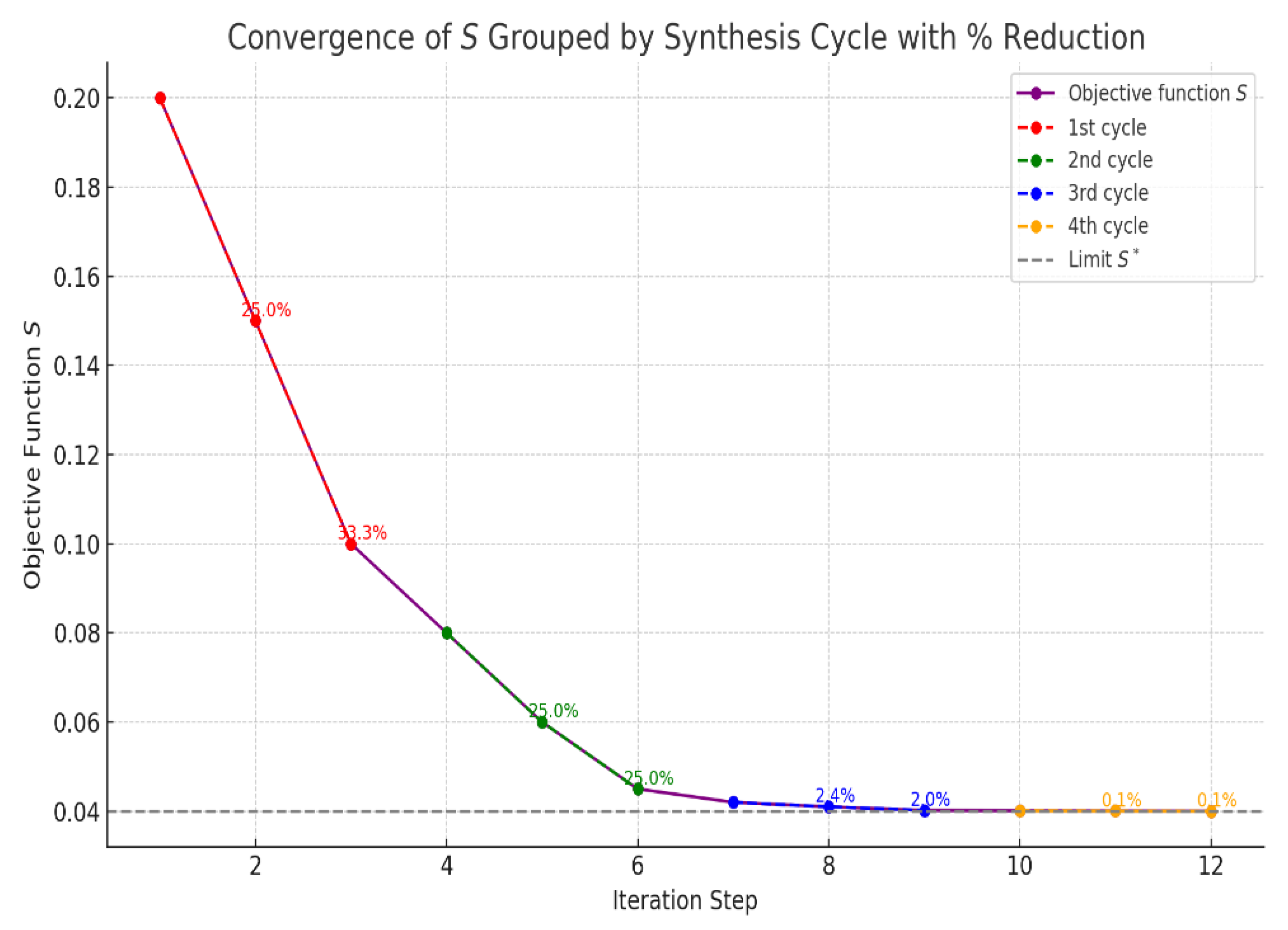
The iterative synthesis algorithm for four-link kinematic chains exhibits a clear pattern of structured convergence, as evidenced by the progressive reduction in the objective function over successive synthesis cycles, as can be seen in Figure 5, Figure 6, Figure 7, Figure 8, Figure 9, Figure 10, Figure 11, Figure 12, Figure 13, Figure 14 and Figure 15 of the algorithm [21]. The graph highlights the sequence , , for each cycle , corresponding to the staged minimization process: solving for the base point , the hinge point , and the endpoint , respectively. Each cycle is plotted in a distinct color, with annotated percentage reductions showing the relative improvement in the objective function after each step. The following observations are noteworthy:
The first synthesis cycle shows significant improvement, with reductions of: 25% from to , 33.3% from to . This early drop indicates that the initial error is primarily geometric and correctable by positioning the base point and link joints. As the algorithm progresses, the percentage reductions become smaller: In the 3rd cycle: 2.4% and 1.9%, In the 4th cycle: less than 0.1%. This behavior confirms that the algorithm approaches a stable local minimum, consistent with the convergence conditions ; ; and . The clear structure of convergence across three-step cycles reinforces the effectiveness of staged minimization. Optimizing over subsets of variables (first , then , then ) ensures that each variable is refined with respect to the updated configuration of the others, yielding a more stable and targeted convergence path [22]. The curve smoothly approaches the limiting value , with no oscillations or reversals. This is a strong indication of numerical stability, proper problem conditioning (as previously verified with , , , and convergence robustness.
The grouped analysis of the convergence curve demonstrates that the synthesis algorithm is both effective and efficient [23]. The structured approach to optimization ensures consistent improvement in each cycle, while the diminishing percentage reductions serve as a natural indicator of when convergence has been achieved. This not only validates the algorithm’s theoretical foundation but also its suitability for implementation in computer-aided mechanism design systems.
7. Discussion
The iterative synthesis procedure employed in this study demonstrates a robust and systematic method for constructing initial four-link kinematic chains based on prescribed plane-parallel displacements of rigid bodies. The algorithm, grounded in approximate kinematic geometry and staged minimization of the weighted difference function , provides significant insights into the geometric and numerical properties of linkage configuration. One of the most significant observations is the consistent and rapid convergence of the objective function across successive iterations. The sequence , , , , , reveals a monotonic decrease in error, validating the effectiveness of the superposition and transformation approach. The convergence criteria involving changes in radius , and base point coordinates fall within the prescribed tolerance after only a few cycles, underscoring the numerical stability of the method. Additionally, the determinant evaluations , , and for the linear systems corresponding to subproblems (solving for points , , and ) were consistently non-zero. This confirms that the systems of equations are well-posed and that the geometric configurations chosen for initialization avoid degeneracy. These determinant checks serve as an important validation step, ensuring that the matrices involved are invertible and that each subproblem yields a unique solution. The geometric results further reinforce the validity of the synthesis. Points and , when plotted relative to the updated point , fall on arcs of circles with radius , maintaining the expected constraint geometry of a four-bar linkage with revolute joints. These visual confirmations complement the numerical convergence and indicate that the synthesized linkage can reliably reproduce the desired relative motions between moving planes and . Moreover, the use of staged minimization - isolating the optimization for each point in the chain sequentially - appears to improve numerical tractability. Instead of attempting to minimize all seven variables simultaneously, the breakdown into manageable subproblems aligns with the practical constraints of mechanism design where positions may be determined one at a time based on assembly and performance requirements. In summary, the results support the conclusion that the proposed method is not only computationally efficient but also geometrically accurate for the synthesis of initial kinematic chains [24,25]. The methodology can be extended to more complex mechanisms or generalized to systems with additional constraints, such as limited joint ranges or dynamic considerations.
8. Conclusions
This work presented a structured methodology for the synthesis of initial four-link kinematic chains with rotational pairs based on the theory of approximate kinematic geometry. The approach involved the specification of relative plane-parallel motion between two moving planes with respect to a fixed base, and the solution of the synthesis problem was carried out by minimizing a weighted geometric deviation function.
Key conclusions from this study are as follows:
- Stable and convergent iterative algorithm:
The proposed iterative algorithm, which minimizes the objective function in three stages (for points , , and ), converges reliably to a local minimum. The observed convergence behavior is smooth, with successive values of decreasing monotonically, and convergence criteria based on the changes in , , and are satisfied within a few iterations.
- 2.
- Well-conditioned linear systems:
The synthesis process is supported by solving three linear systems (corresponding to systems Eq. (17), Eq. (21), and Eq. (24)), and determinant testing confirmed that the systems are non-singular , , for the provided input configurations. This indicates that the algorithm is numerically stable and the synthesis conditions are well-posed.
- 3.
- Geometrical accuracy of link placement:
The positions of the synthesized points and relative to the base lie on circles of radius , verifying the geometrical correctness of the linkage design. The visualizations show that the synthesized four-link mechanism satisfies the constraints of consistent angular displacements and relative orientations.
- 4.
- Modular and extendable framework:
The methodology allows for modular implementation, with each synthesis step being independently solvable and verifiable. This makes it especially suitable for computer-aided mechanism design applications and opens up possibilities for extension to mechanisms with translational joints or higher degrees of freedom.
- 5.
- Effective error minimization strategy:
The use of staged error minimization - optimizing each subset of variables sequentially - reduces computational complexity while maintaining synthesis accuracy. This approach provides a practical and scalable solution for the synthesis of planar mechanisms.
In summary, the developed algorithm offers a reliable, accurate, and computationally efficient technique for the synthesis of initial four-link mechanisms under geometrical motion constraints. It serves as a solid foundation for further developments in mechanism synthesis, including the integration of dynamic constraints, optimization under workspace limitations, and generalization to spatial linkages.
Author Contributions
Conceptualization, A.Z.; methodology, A.Z.; software, A.Z.; validation, K.A.; formal analysis, A.A. and Y.Y.; investigation, Z.A.; resources, G.S. and Y.Y.; data curation, A.O.; writing—original draft preparation, Z.A., A.Z., Y.Y., and K.A.; writing—review and editing, A.A., G.S., and A.O.; visualization, Z.A. and A.O.; supervision, A.Z.; project administration, Z.A., A.Z.; Y.Y. and A.A.; funding acquisition, K.A., G.S., A.A., and A.O. All authors have read and agreed to the published version of the manuscript.
Funding
This research was funded by Almaty University of Power Engineering and Telecommunications named after Gumarbek Daukeyev, grant number AP19677356.
Institutional Review Board Statement
The study did not require ethical approval.
Informed Consent Statement
Not applicable.
Data Availability Statement
Data are contained within the article.
Acknowledgments
This work has been supported financially by the research project (To develop systems for controlling the orientation of nanosatellites with flywheels as executive bodies based on linearization methods) of the Ministry of Education and Science of the Republic of Kazakhstan and was performed at Research Institute of Communications and Aerospace Engineering in Almaty University of Power Engineering and Telecommunications named after Gumarbek Daukeyev, which is gratefully acknowledged by the authors.
Conflicts of Interest
The authors declare no conflicts of interest.
References
- Abdreshova, S.; Zhauyt, A.; Alipbayev, K.; Kosbolov, S.; Aden, A.; Orazaliyeva, A. Synthesis of Four-Link Initial Kinematic Chains with Spherical Pairs for Spatial Mechanisms. Appl. Sci. 2025, 15, 3602. [Google Scholar] [CrossRef]
- Che, L. X.; Chen, G. W.; Jiang, H. Y.; Du, L.; Wen, S. K. Dimensional synthesis for a Rec4 parallel mechanism with maximum transmission workspace. Mech. and Mach. Theor. 2020, 153, 104008. [Google Scholar] [CrossRef]
- Liu, W.; Liu, H.Z. Synthesis of asymmetric parallel mechanism with multiple 3-DOF motion modes. Adv. Mech. Eng. 2022, 14, 2–1. [Google Scholar] [CrossRef]
- Copeland, Z.A. Continuous approximate kinematic synthesis of planar, spherical, and spatial four-bar function generating mechanisms. Ph.D. dissertation, Carleton University, Ottawa, Ontario, Canada, April 26, 2024.
- Freudenstein, F. Structural error analysis in plane kinematic synthesis. J. of Engin. for Indus. 1959, 81, 15–21. [Google Scholar] [CrossRef]
- Freudenstein, F. Approximate synthesis of four-bar linkages. Trans. of the ASME 1955, 77, 853–861. [Google Scholar] [CrossRef]
- Rao, S.; Ambekar, A. Optimum design of spherical 4-R function generating mechanisms. Mech. and Mach. Theor. 1974, 9, 405–410. [Google Scholar] [CrossRef]
- Kong, X. Reconfiguration analysis of a 3-DOF parallel mechanism using Euler parameter quaternions and algebraic geometry method. Mech Mach Theory 2014, 74, 188–201. [Google Scholar] [CrossRef]
- Gogu, G. Structural synthesis of parallel robots. Part I: methodology. Solid Mech Appl 2012, 149, 653–663. [Google Scholar]
- Alizade, R.; F. C. Can, F. C.; Kilit, O. Least square approximate motion generation synthesis of spherical linkages by using chebyshev and equal spacing. Mech. and Mach. Theo. 2013, 61, 123–135. [CrossRef]
- Alizade, R.; Bayram, C. Structural synthesis of parallel manipulators. Mech. and Mach. Theo. 2004, 39, 857–870. [Google Scholar] [CrossRef]
- Zhao, J.S.; Zhou, K.; Feng, Z.J. A theory of degrees of freedom for mechanisms. Mech. and Mach. Theo. 2004, 39, 621–643. [Google Scholar] [CrossRef]
- Zhao, J.; Feng, Z.; Chu, F.; Ma, N. Structure synthesis of spatial mechanisms. Adv. The. of Cons. and Mot. Analy. for Rob. Mech. 2014, 367–396, Book Chapter. [Google Scholar] [CrossRef]
- Tultayev, B.; Balbayev, G.; Zhauyt, A.; Sultan, A.; Mussina, A. Kinematic synthesis of mechanism for system with a technical vision. MATEC Web of Conferences 2018, 237, 03009. [Google Scholar] [CrossRef]
- Liao, Z.; Tang, S.; Wang, D. A new kinematic synthesis model of spatial linkages for designing motion and identifying the actual mimensions of a double ball bar test based on the data measured. Machines 2023, 11, 919. [Google Scholar] [CrossRef]
- Faizov, M.; Fanil, Kh. Computations analysis of a four-link spherical mechanism for a spatial simulator. Vestnik Moskovskogo Aviatsionnogo Instituta 2020, 27, 196–206. [Google Scholar] [CrossRef]
- Grimm, E.M.; Andrew, P.M.; Michael, L.T. Software for the kinematic synthesis of coupler-driven spherical four-bar mechanisms. In ASME 2007 International Design Engineering Technical Conferences and Computers and Information in Engineering Conference. ASMEDC, 2007. [CrossRef]
- Vilas, C. P. Optimal synthesis of adjustable four-link planar and spherical crank-rocker type mechanisms for approximate multi-path generation. Thesis. 2013. Available online: http://etd.iisc.ac.in/handle/2005/3319.
- Vilas, C. P.; Michael, A.A. F.; Ashitava, G. Synthesis of adjustable spherical four-link mechanisms for approximate multi-path generation. Mech. Mach. The. 2013, 70, 538–552. [Google Scholar] [CrossRef]
- Yao, J.; and Jorge, A. The kinematic synthesis of steering mechanisms. Trans. of the Canad. Soci. for Mech. Eng. 2000, 24, 453–476. [Google Scholar] [CrossRef]
- Acar, O.; Hacı, S.; and Ziya, S. Measuring curvature of trajectory traced by coupler of an optimal four-link spherical mechanism. Measurement 2021, 176, 109189. [Google Scholar] [CrossRef]
- Hunt, K.H. Kinematic Geometry of Mechanisms; Oxford University Press: Oxford, UK, 1978. [Google Scholar]
- Huang, X.; Liu, C.; Xu, H.; Li, Q. Displacement analysis of spatial linkage mechanisms based on conformal geometric algebra. J. Mech. Eng. 2021, 57, 39–50. [Google Scholar]
- Wang, D.; Wang, W. Kinematic Differential Geometry and Saddle Synthesis of Linkages; John Wiley & Sons: Singapore, 2015. [Google Scholar]
- Wang, D.; Wang, Z.; Wu, Y.; Dong, H.; Yu, S. Invariant errors of discrete motion constrained by actual kinematic pairs. Mech. Mach. Theory 2018, 119, 74–90. [Google Scholar] [CrossRef]
Figure 1.
Configurations of synthesized initial kinematic chains: closed four-bar link chain (ABCD) and open variants (ACD, ABD).
Figure 1.
Configurations of synthesized initial kinematic chains: closed four-bar link chain (ABCD) and open variants (ACD, ABD).
Figure 2.
Configurations of ACD and AD kinematic chains with translational pairs.
Figure 3.
Configurations of ABD and AD kinematic chains with translational pairs.
Figure 4.
The algorithm visualizes the entire iterative synthesis algorithm for four-link kinematic chains with rotational pairs, showing each computational step and convergence condition clearly.
Figure 4.
The algorithm visualizes the entire iterative synthesis algorithm for four-link kinematic chains with rotational pairs, showing each computational step and convergence condition clearly.
Figure 5.
The 2D plot showing the initial positions of the points: shown as a red circle, and shown as a blue square, a dashed line connects them to indicate their initial relative position.
Figure 5.
The 2D plot showing the initial positions of the points: shown as a red circle, and shown as a blue square, a dashed line connects them to indicate their initial relative position.
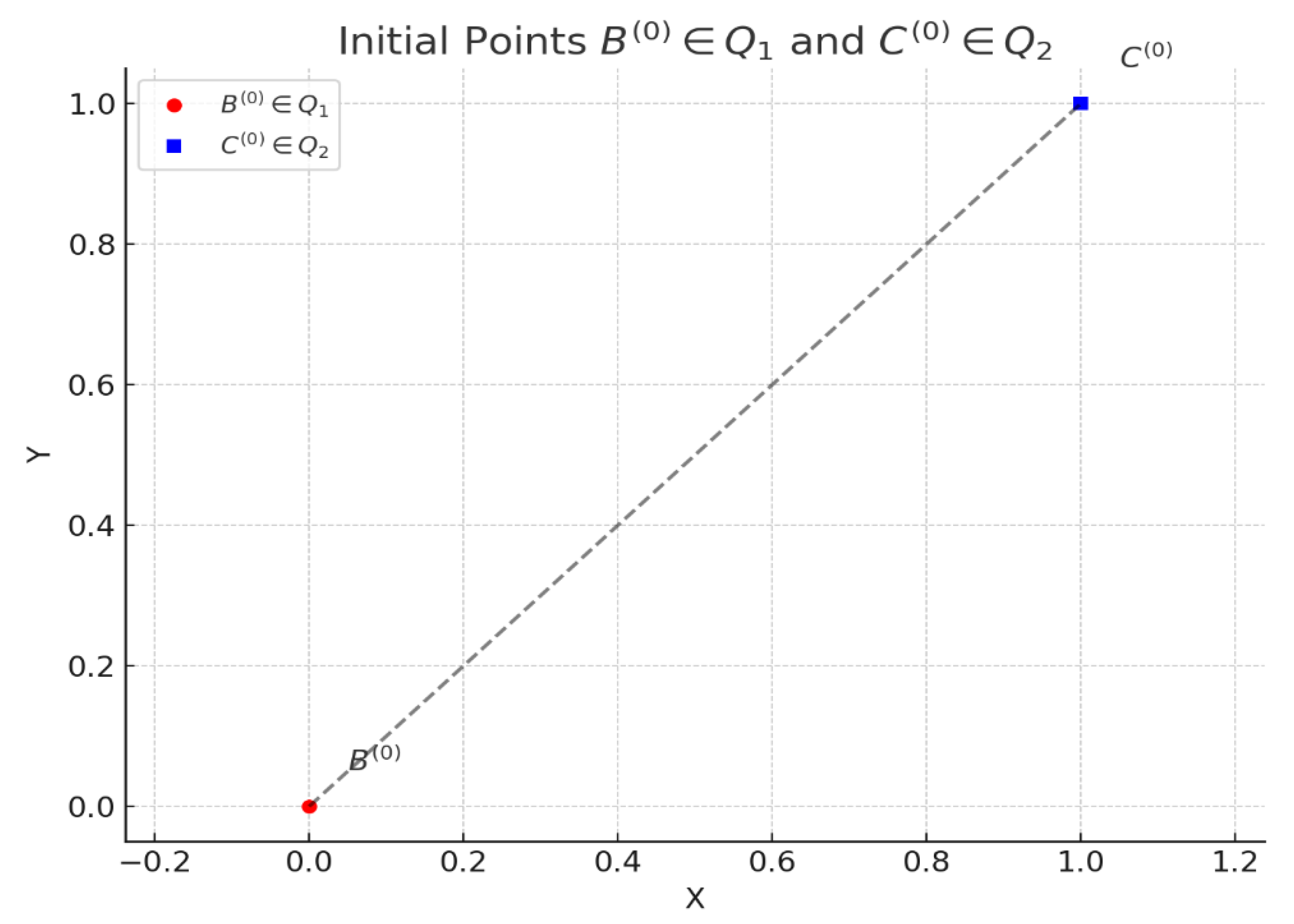
Figure 6.
This confirms the system is non-singular and suitable for performing the basic iterative synthesis step. The matrix for system Eq. (17) has a non-zero determinant: .
Figure 6.
This confirms the system is non-singular and suitable for performing the basic iterative synthesis step. The matrix for system Eq. (17) has a non-zero determinant: .
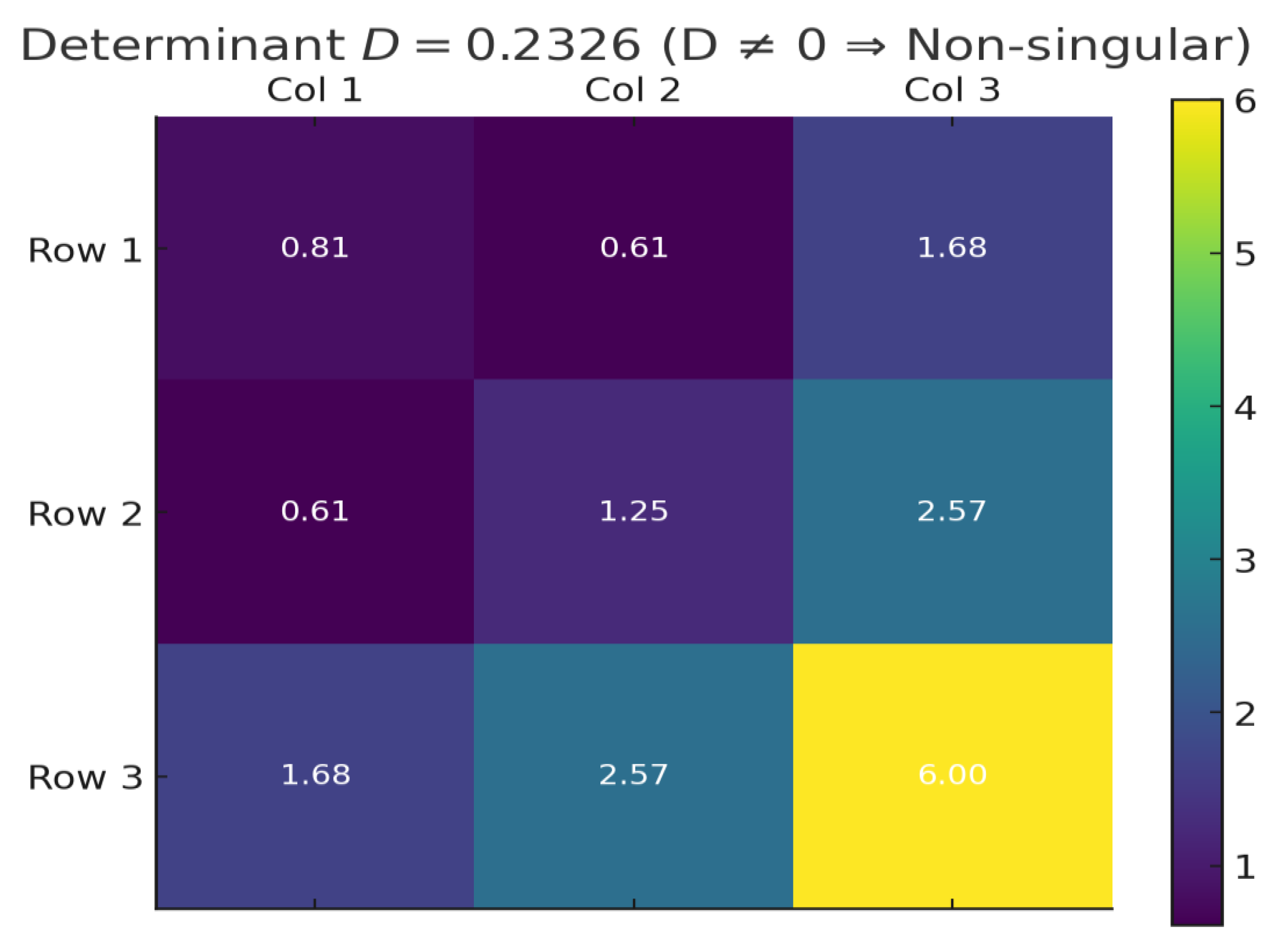
Figure 7.
This 2D plot shows: the computed base point from the synthesis step; and two points lying on a circle of radius around ; Dashed lines represent the virtual links connecting to both and .
Figure 7.
This 2D plot shows: the computed base point from the synthesis step; and two points lying on a circle of radius around ; Dashed lines represent the virtual links connecting to both and .
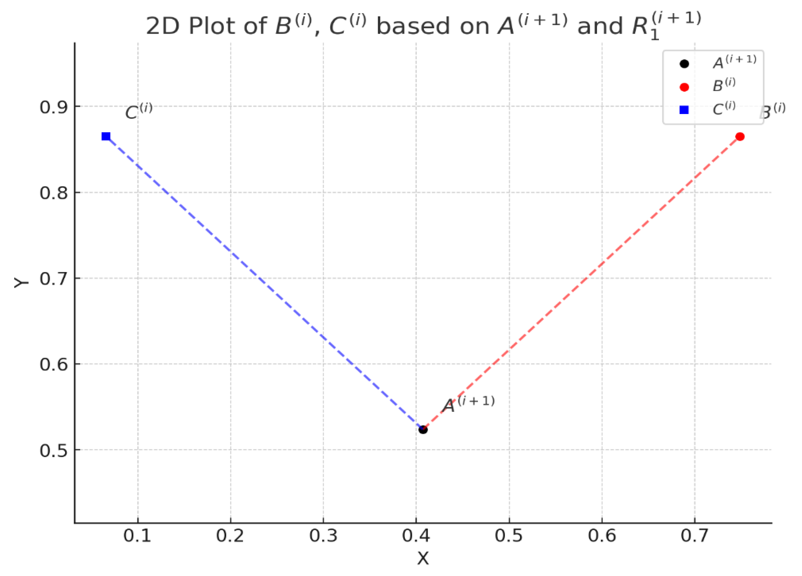
Figure 8.
This confirms the system is non-singular and solvable, and the computed values are valid for continuing the synthesis process. Results of the basic iterative synthesis step: , , . Determinant .
Figure 8.
This confirms the system is non-singular and solvable, and the computed values are valid for continuing the synthesis process. Results of the basic iterative synthesis step: , , . Determinant .
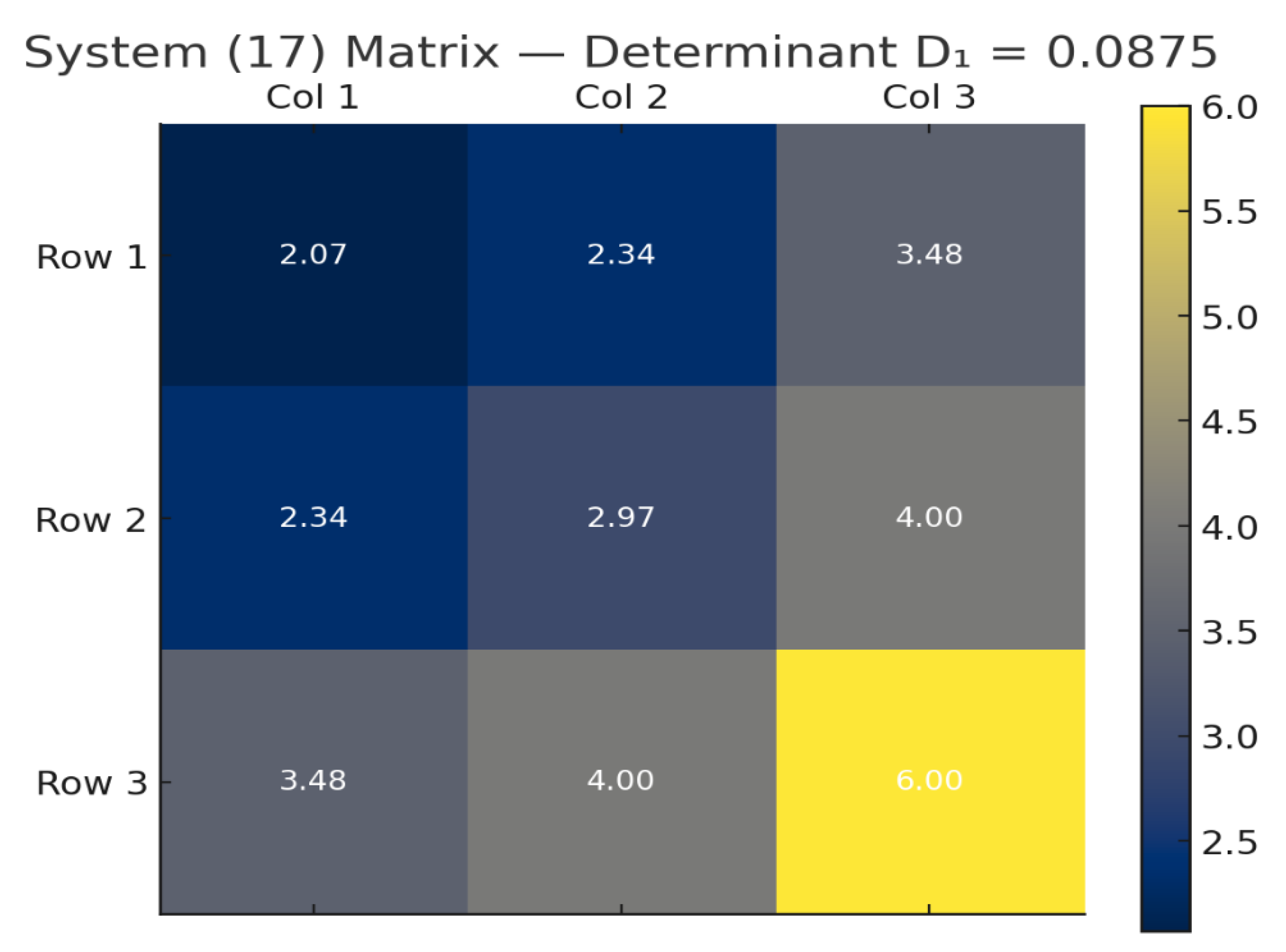
Figure 9.
This 2D plot visualizes the synthesis step using: the updated base point; the new hinge point derived from system Eq. (21); the previous point on the second moving plane; Dashed line: shows the synthesized link between and ; Black dashed line: represents the connection to the known point .
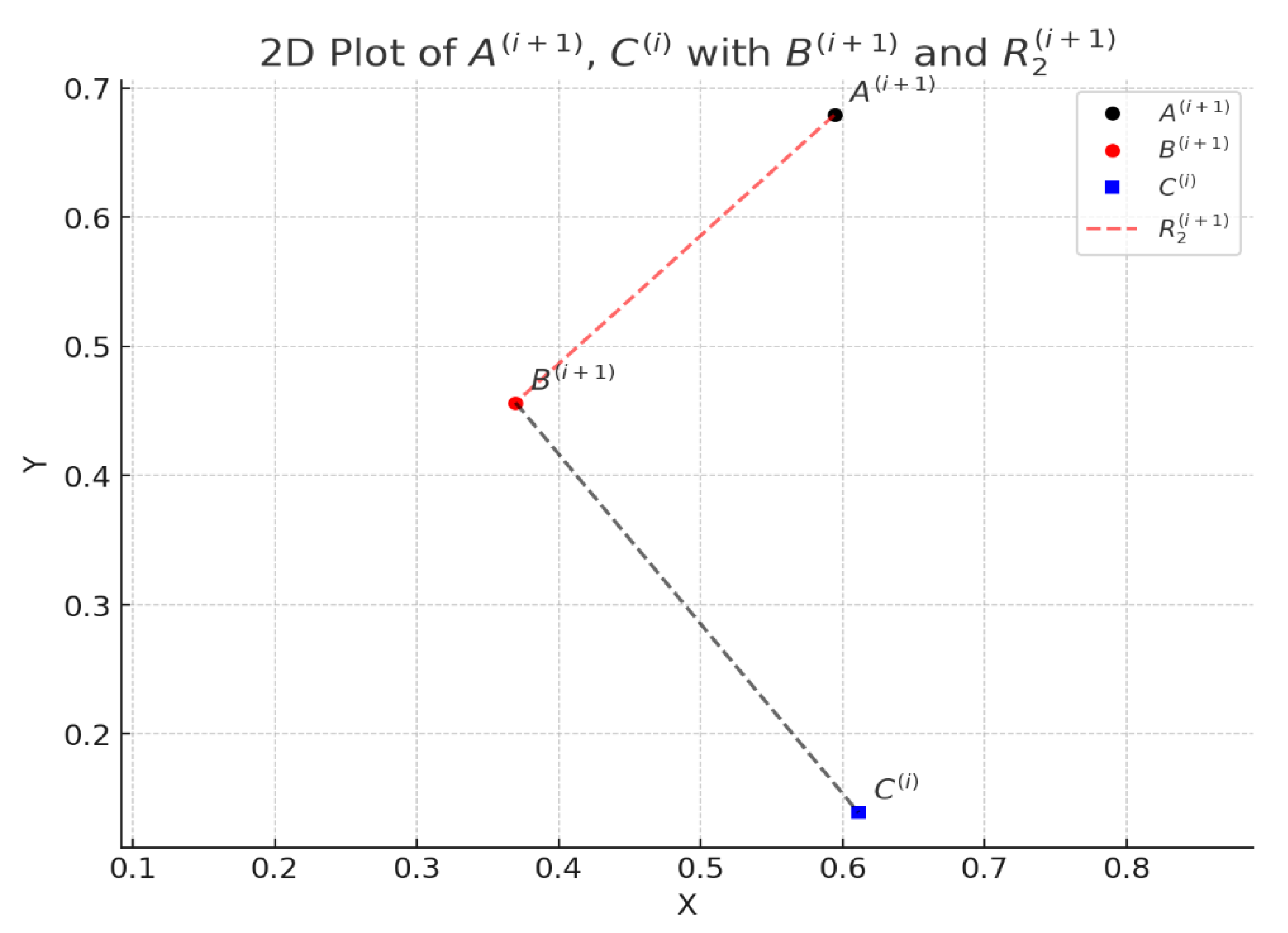
Figure 10.
The 2D heatmap shows the coefficient matrix used in system Eq. (21) for the second synthesis step. Results of the basic iterative synthesis step: , , . Determinant .
Figure 10.
The 2D heatmap shows the coefficient matrix used in system Eq. (21) for the second synthesis step. Results of the basic iterative synthesis step: , , . Determinant .
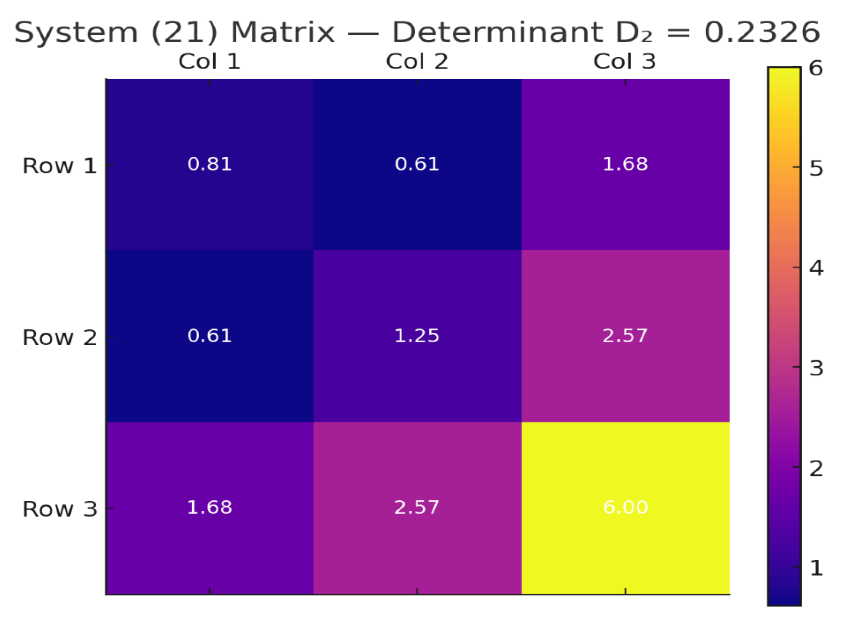
Figure 11.
This 2D plot completes the synthesis step by showing: the fixed base point; the intermediate hinge point; computed along the extended direction from through , at distance ; Dashed lines indicate the link segments: red for , blue for .
Figure 11.
This 2D plot completes the synthesis step by showing: the fixed base point; the intermediate hinge point; computed along the extended direction from through , at distance ; Dashed lines indicate the link segments: red for , blue for .
Figure 12.
The 2D heatmap above visualizes the coefficient matrix used in system Eq. (24) for the final step of your synthesis loop. Results of the final iterative step: , , . Determinant .
Figure 12.
The 2D heatmap above visualizes the coefficient matrix used in system Eq. (24) for the final step of your synthesis loop. Results of the final iterative step: , , . Determinant .
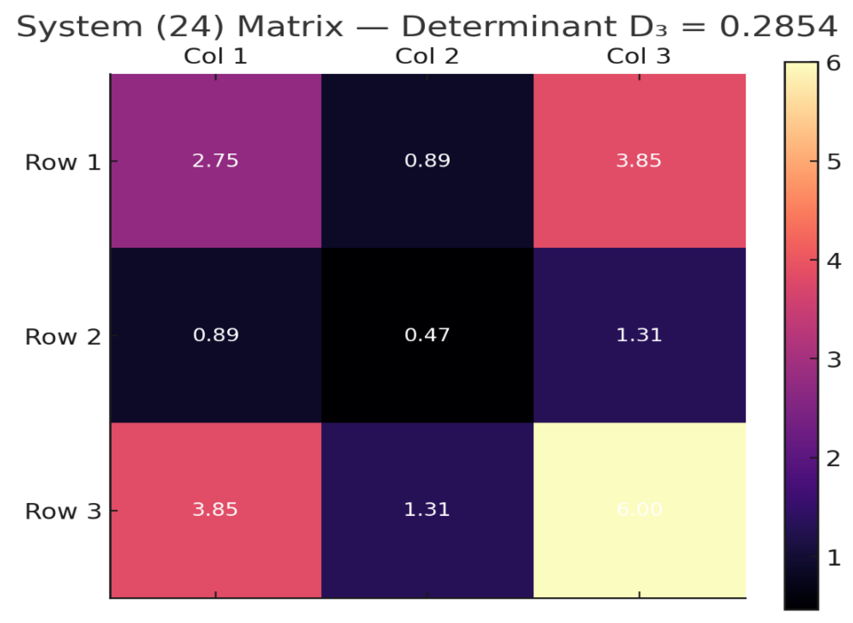
Figure 13.
This 2D plot visualizes the convergence behavior of the iterative synthesis process: Red line change in link length ; Green line: change in base point x-coordinate ; Blue line: change in base point y-coordinate ; The black dashed line shows the threshold . As the iterations progress, all three quantities approach or drop below the threshold — confirming convergence.
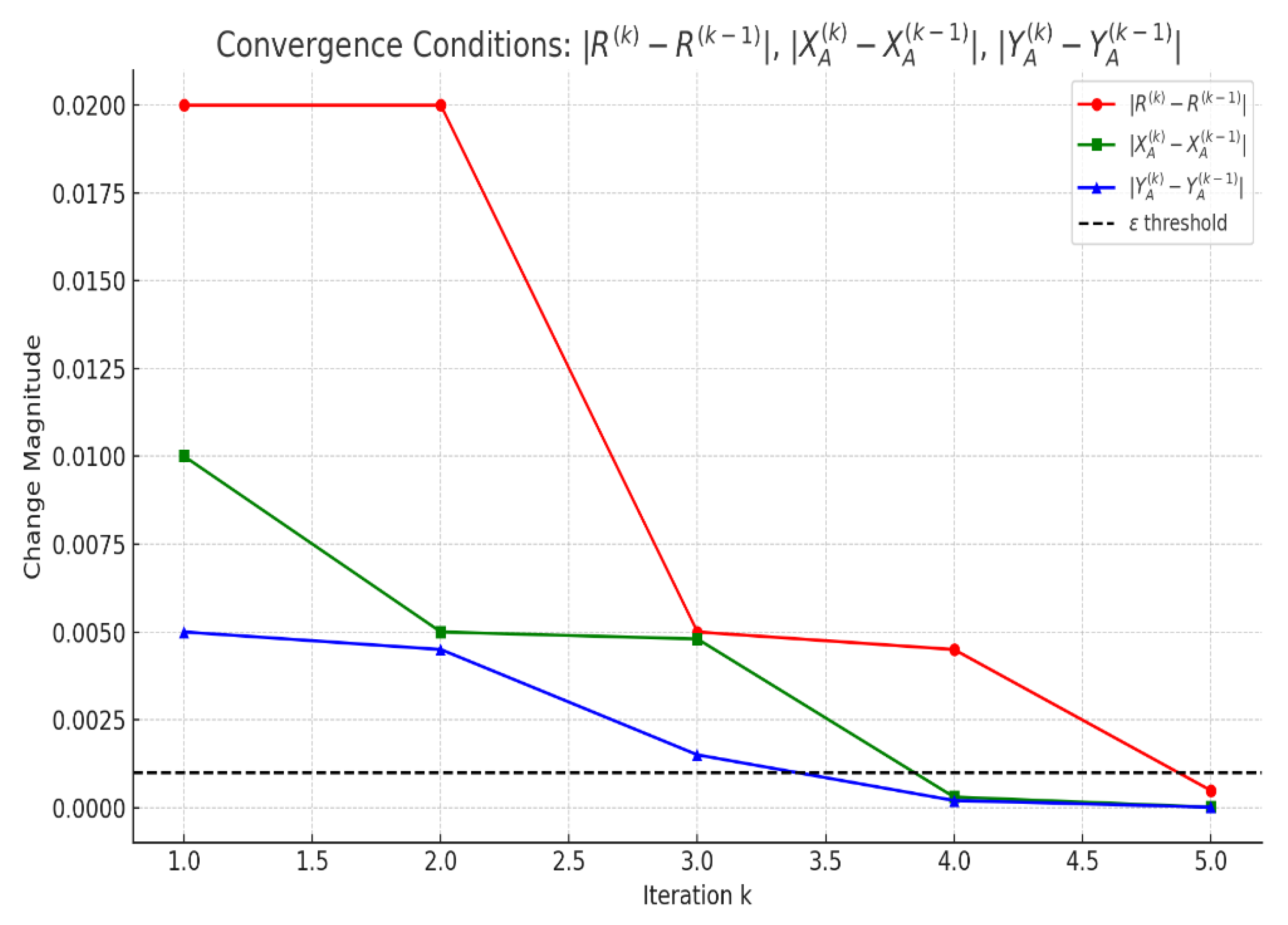
Figure 14.
This 2D plot shows the convergence of the objective function over successive synthesis stages: Each point represents a step in the optimization (e.g., solving for , then , then ); The gray dashed line shows the limit , the locally minimized value of the function.
Figure 14.
This 2D plot shows the convergence of the objective function over successive synthesis stages: Each point represents a step in the optimization (e.g., solving for , then , then ); The gray dashed line shows the limit , the locally minimized value of the function.
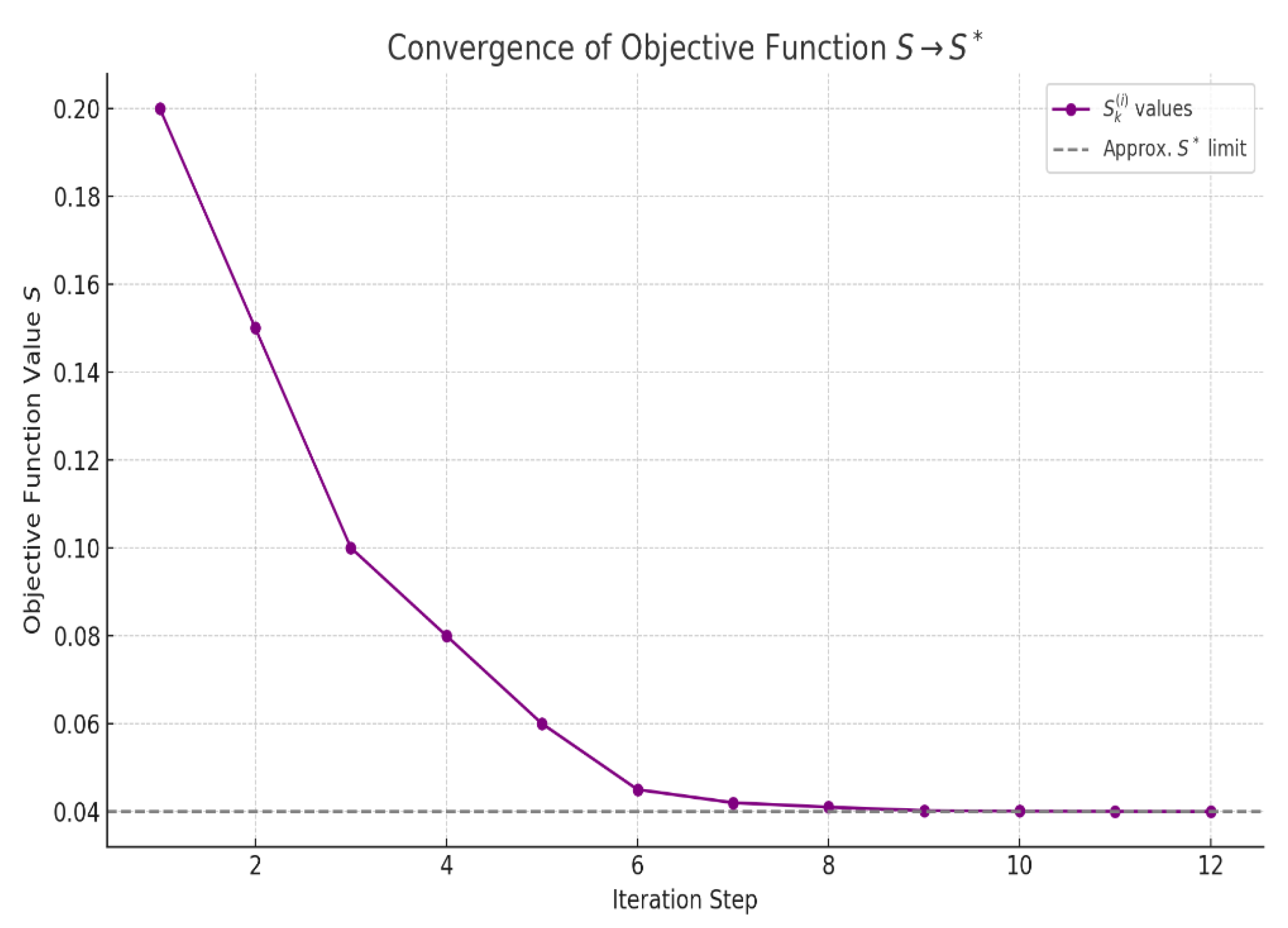
Figure 15.
This graph illustrates the convergence of the objective function across four synthesis cycles, with each cycle consisting of three steps: solving for , , and . Each color-coded segment represents one synthesis cycle: Red 1st cycle ; Green 2nd cycle ; Blue 3rd cycle ; Orange 4th cycle . Percentage reductions between each stage are annotated beside the markers, showing effective drop in error per synthesis step. The dashed horizontal line represents the asymptotic limit , confirming convergence of the objective function.
Disclaimer/Publisher’s Note: The statements, opinions and data contained in all publications are solely those of the individual author(s) and contributor(s) and not of MDPI and/or the editor(s). MDPI and/or the editor(s) disclaim responsibility for any injury to people or property resulting from any ideas, methods, instructions or products referred to in the content. |
© 2025 by the authors. Licensee MDPI, Basel, Switzerland. This article is an open access article distributed under the terms and conditions of the Creative Commons Attribution (CC BY) license (http://creativecommons.org/licenses/by/4.0/).
Copyright: This open access article is published under a Creative Commons CC BY 4.0 license, which permit the free download, distribution, and reuse, provided that the author and preprint are cited in any reuse.


