
Submitted:
01 May 2025
Posted:
02 May 2025
You are already at the latest version
Abstract
Defect remediation on custom-curved glulam beams is still performed manually because knots are irregular, numerous, and located on elements that cannot pass through linear production lines, limiting the scalability of timber-based architecture. This study presents Woodot, an autonomous mobile robotic platform that combines an omnidirectional rover, a 6-dof collaborative arm, and a fine-tuned Segment Anything computer-vision pipeline to identify, mill, and plug surface knots on geometrically variable beams. The perception model was trained on a purpose-built micro-dataset and reached an F1 score of 0.69 on independent test images, while the integrated system located defects with 4.3 mm mean positional error. Full remediation cycles averaged 74 s per knot, reducing processing time by more than 60 % compared with skilled manual operations, and achieved flush plug placement in 87 % of trials. These outcomes demonstrate that a lightweight AI model coupled with mobile manipulation can deliver reliable, shop-floor automation for low-volume, high-variation timber production. By shortening cycle times, lowering worker exposure to repetitive tasks, and minimising material waste, Woodot offers a vi-able pathway to enhance the environmental, economic, and social sustainability of digital timber construction.
Keywords:
high payload cobots
; mobile robotics for unstructured environments
; computer vision
; defect recognition
; fine-tuning segmentation model
; AI-based visual inspection
; glulam defect remediation
; sustainable timber construction
1. Introduction
The global shift toward low-carbon construction has renewed interest in engineered timber, whose high strength-to-weight ratio and capacity to sequester biogenic carbon make it a strategic material for sustainable buildings. Laminated timber beams, and especially custom-curved glulam elements used in free-form architecture, embody this potential but also expose a critical bottleneck: the manual remediation of surface knots. Although knots seldom impair structural performance, their dark colour and irregular texture diminish the visual quality demanded for exposed structural members. Current practice—hand-drilling each knot and inserting a wooden plug—remains labour-intensive, ergonomically taxing, and difficult to scale, particularly when large, non-linear beams cannot pass through straight production lines.
Researchers have therefore explored automated surface inspection. Early colour and texture segmentation methods achieved limited robustness across species and finishes [1,2]. Recent convolutional and transformer-based detectors outperform human inspectors in speed and repeatability [3,4]. In parallel, industrial robotics has been adopted for sanding, routing, and finishing, yet almost always in static, fixture-based cells suited to planar panels or prismatic parts [5,6]. Such systems struggle with geometric diversity, random placement, and metre-scale curvature typical of bespoke glulam.
Two divergent strategies are now debated. One stream argues for ever larger fixed cells with sophisticated fixtures, maintaining conventional factory layouts; the other advocates mobile, human-scale robots that travel to the part, trading rigidity for flexibility. The latter has gained traction in aerospace and composite repair, where climbing or rover-mounted manipulators conduct in-situ inspection and milling [7,8]. Whether this paradigm can meet the payload, precision, and safety requirements of timber fabrication, however, remains an open question.
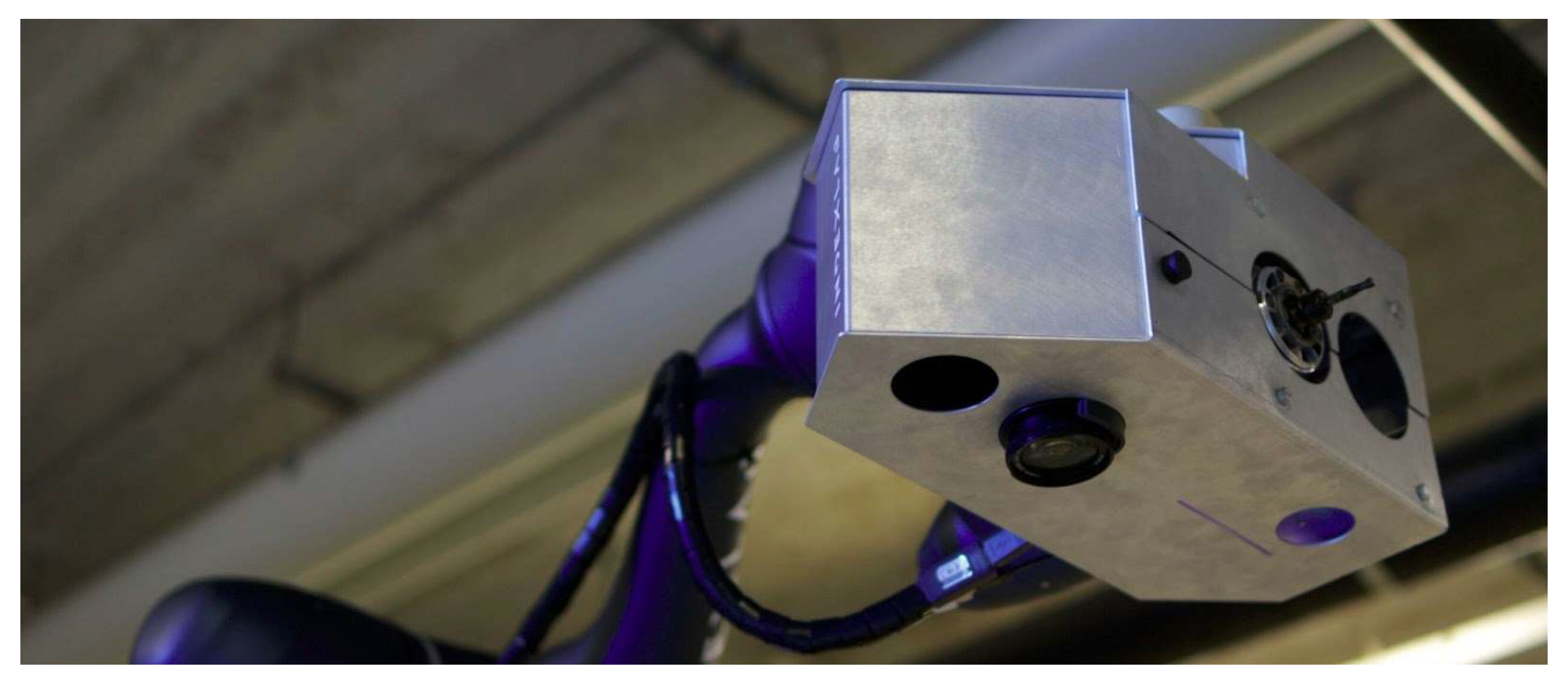
This work addresses that gap by presenting Woodot (Figure 1), an autonomously navigating rover equipped with a six-degree-of-freedom collaborative arm and an AI-driven vision pipeline. The system (i) detects knots on curved beams using a fine-tuned Segment Anything model trained on a lightweight, domain-specific dataset, (ii) mills the defect, and (iii) inserts a matching plug—all without beam repositioning or human guidance. We show that Woodot locates defects with 4.3 mm mean error, completes a full remediation cycle in 74 s (over 60 % faster than skilled manual labour), and achieves flush plug seating in 87 % of trials.
By demonstrating reliable, shop-floor automation for low-volume, high-variation timber production, Woodot contributes a scalable route to (a) reducing material waste, (b) lower worker exposure to repetitive tasks, and (c) support wider adoption of carbon-beneficial timber architecture.
2. Materials and Methods
This section details the hardware, software, datasets, and operational workflow used to implement the Woodot system. All source code, trained weights, and raw datasets are openly available at Zenodo repository under the accession number 10.5281/zenodo.15304349, and it is publicly available at: https://doi.org/10.5281/zenodo.15304349.
2.1. System Overview
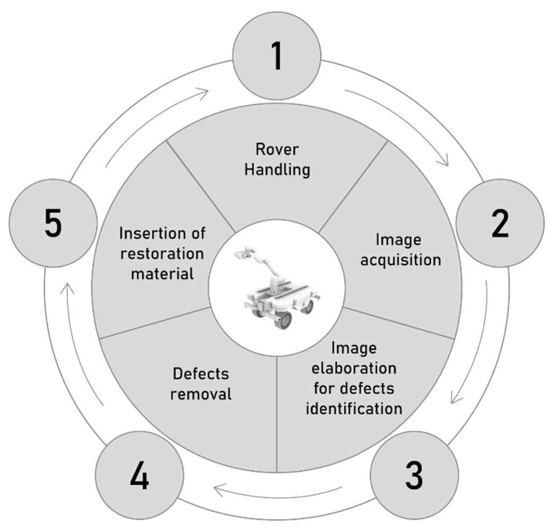
Woodot comprises an omnidirectional mobile base, a 6-degree-of-freedom collaborative arm, a combined camera–router end-effector, and a Docker-orchestrated control stack. Five subsystems execute the remediation workflow: (i) rover handling, (ii) image acquisition, (iii) vision-based defect identification, (iv) milling of the knot, and (v) insertion of a wooden plug.
Figure 3.
The five key subsystems of Woodot.
2.2. Hardware Infrastructure
The hardware for the Woodot application is integrated using a Dell Inspiron 7577 as the host machine. This computer has 16.0 GiB of RAM memory and features an Intel Core i7-7700HQ processor with eight cores and a dedicated NVIDIA GeForce GTX 1060 graphics card.
The mobile base of Woodot is based on the same autonomous robotic rover described in Ruttico et al. [9]. It is a lightweight and flexible platform designed for navigation in unstructured environments. The rover is equipped with four independently driven and steered wheels, allowing for omnidirectional movement, including lateral and diagonal translation and zero-radius rotation. This high maneuverability is essential when the rover is near large timber beams in constrained spaces such as carpentry workshops or warehouses.
The system is powered by rechargeable lithium-ion batteries and features all-electric components, ensuring quiet and emission-free operation. Integrated with industrial-grade safety sensors and LiDARs, the rover is capable of autonomous navigation while avoiding obstacles and maintaining safe distances from human operators. The onboard control unit enables seamless switching between manual teleoperation and fully autonomous modes.
Figure 4.
The three main components of Woodot: the rover, the robot, the end-effector.
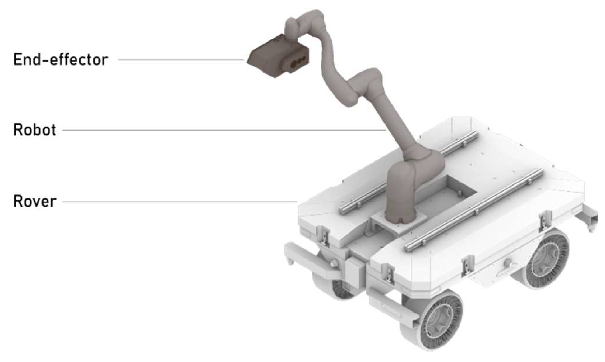
The vehicle integrates a collaborative robotic arm (Doosan model H2515) mounted at the center top to ensure optimal balance and reach.
The H2515 is part of the H-SERIES and is a collaborative 6-dof robot with a payload capacity of 25 kg and an operating radius of 1500mm. It features 6 high-performance torque sensors and operates efficiently with low electrical power consumption. The maximum linear TCP speed is 1 m/s, and it has a repeatability of ±0.1 mm. The operating temperature ranges from 0 °C to 45 °C. The I/O power supply operates at 24V and 3A.
The control box measures 490 x 390 x 287 mm and weighs 9 kg, and it has been integrated on top of the rover chassis. It provides 16 digital inputs, 16 digital outputs, 2 analog inputs, and 2 analog outputs, also powered by a 24V supply. Communication options include Serial (RS232), USB 3.0 (RS422/485), TCP/IP, Modbus-TCP (Master/Slave), Modbus-RTU (Master), EtherNet/IP (Adapter), and PROFINET IO (Device).
Mechanical and structural adaptations were made to the rover chassis to support the arm’s dynamic loads during tool operations. Communication between the rover and the arm controller is handled via Modbus TCP, with synchronization based on shared state machines and waypoint logic.
An inverter was installed to convert the battery voltage of 48V DC into alternating current at 220V AC and 50 Hz, which is essential for powering the Doosan controller. A PLC has been installed to facilitate communication between the onboard PC, the host machine, and the Doosan controller, and the safety of the Doosan controller is connected to the Rover safety PLC to ensure proper safety measures are in place.
The case of the choice of a collaborative robot over an industrial robot goes beyond the natural perks of selecting the least heavy machine with the highest payload. While these perks - the reduction of energy demand and the integration flexibility for future fabrication techniques - may be enough to make a prototype work, choosing a collaborative robot over an industrial robot is generally part of a multifold strategy [10] to scale the application to an industrial level.
The paradigm shifts from ensuring the industrial robot-human interaction is as infrequent as possible, pointing toward a fully automated solution, to actually merging the productivity of robotic systems with the flexibility and dexterity of manual ones [11], ensuring there are always “safe collaboration areas” between robot and operator.
In fact, cobots are great for high-mix, low-volume production environments as they enable a more flexible division of tasks, without the need for safety cages. They employ advanced safety features such as force and torque sensors, to allow them to detect collisions and stop immediately, and built-in speed and force limits [10]. Drag-and-drop interfaces, hand-guided teaching, and no-code or low-code environments ensure cobots are easier to set up and use and don’t require robotics expertise for an unskilled operator in programming.
This user-friendliness significantly reduces the deployment time compared to industrial robots, particularly when equipped with computer vision systems that allow them to navigate unstructured environments, changing their layout rapidly, so they’re perfect for small & medium enterprises to scale automation in a gradual and controlled way.
Figure 5.
The different end-effector configurations integrate camera, router and wood plugs in an aluminum carter.
Figure 5.
The different end-effector configurations integrate camera, router and wood plugs in an aluminum carter.
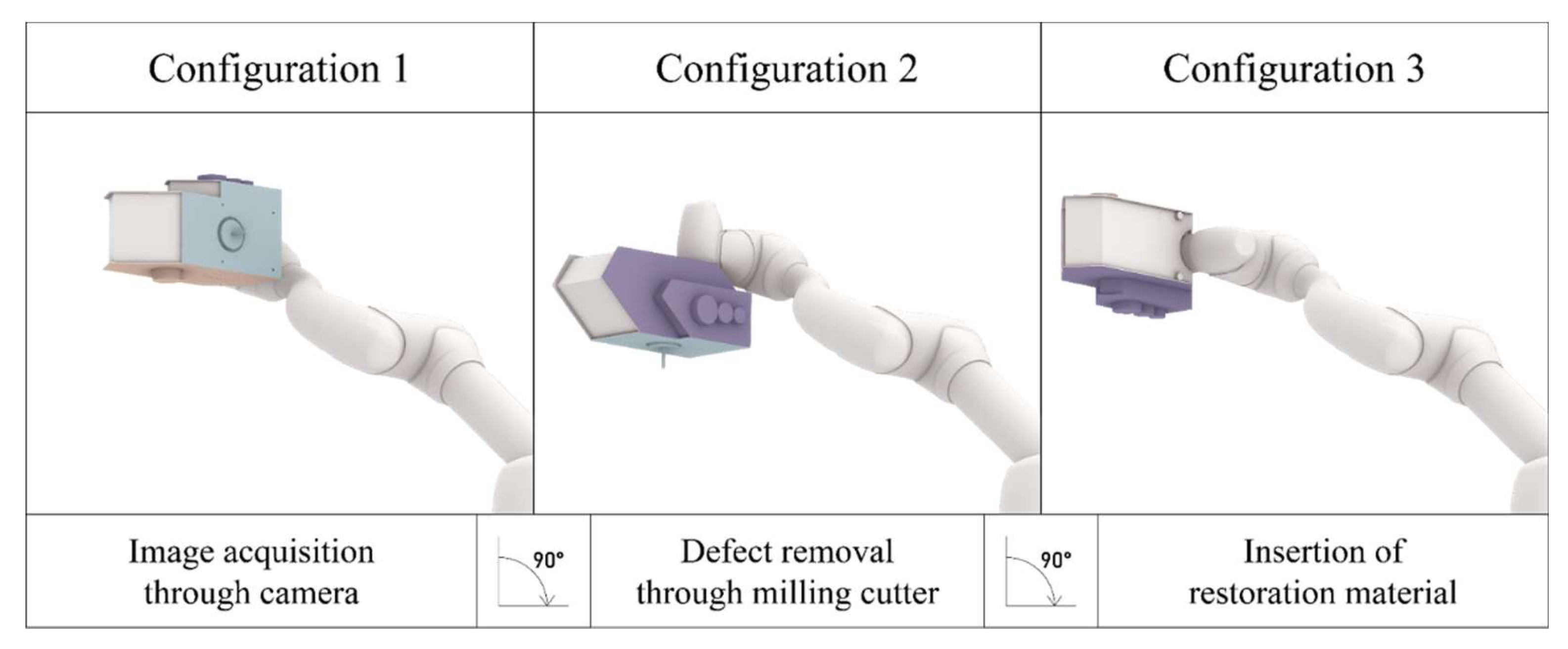
At the end of the Doosan robotic arm, a custom end-effector integrating a Canon EOS 1200D DSLR equipped with a standard EF-S 18–55 mm lens camera, a DeWalt D26200-GB 8mm Fixed Base Router, and a wooden plug dispenser is attached to the flange.
The Canon EOS 1200D is an entry-level digital single-lens reflex camera. At its core, the camera features an 18-megapixel APS-C-sized CMOS sensor, which produces images at a maximum resolution of 5184 x 3456 pixels. With this sensor, the camera provides a native ISO range from 100 to 6400, extendable up to ISO 12800, enabling it to perform in varied lighting conditions.
The camera supports a maximum shutter speed of 1/4000th of a second and can capture continuous shots at around 3 frames per second. Its exposure system provides various modes, including shutter and aperture priority, as well as manual controls, and includes essential features like exposure compensation and built-in digital bracketing options. Focusing is facilitated by a basic system of 9 autofocus (AF) points.
Connectivity with the camera is limited to a USB 2.0 interface and HDMI output, without any built-in wireless options. Physically, the camera maintains a compact DSLR form factor with dimensions of approximately 130x100x78 mm and weighs around 480 grams.
It is interesting to note that, for defect recognition on a flat, planar surface, even monocular cameras, such as high-resolution DSLRs, are often preferable to a stereo camera setup. Since the surface is flat, the depth information can be inferred from the 2D image data alone, eliminating the need for the more complex stereo disparity calculations, making the overall system simpler, more compact, and potentially more cost-effective, as only a single camera is required. Additionally, the entire computation time of image segmentation, milling trajectory calculation, and robot feedback rate is significantly faster, even on a consumer notebook GPU. A DSLR camera can provide significantly higher image resolution compared to many stereo camera systems, which can be very advantageous for a detailed morphological analysis of the defect.
The D26200-GB [17] is a fixed base router with an 8mm collet size and a 900W motor, powered by 240V mains. It features full-wave electronic speed control to maintain the selected speed under all loads and offers variable speeds between 16,000 and 27,000 RPM to match different materials. It has aluminium motor housing and weighs around 2kg.
The router supports cutter diameters up to 30mm. The milling spindle that was mounted at its end is a CMT Orange Tools Solid Carbide Downcut Spiral Bit (190.080.11) featuring 8mm diameter, 80mm of total length, 32mm of cutting length, and low-angle spiral cutting edges that are designed specifically to shear wood cleanly and provide efficient chip ejection.
2.3. Software Infrastructure
At the heart of Woodot is a Docker infrastructure of microservices designed to automate the defect recognition and milling processes.
The operating system running transversally as base for every Docker service is Ubuntu 24.04.1 LTS, 64-bit, with a firmware version of 1.17.0, running GNOME version 46 and using the X11 windowing system, with a kernel version of Linux 6.8.0- 41-generic. The host machine runs Windows 10.
These services involve the monitoring of the rover’s state, the acquisition and processing of camera images, and the control of a robotic arm and its end-effector. In between, a simulation environment in Grasshopper3D [15], a popular visual programming environment for 3D modeling and analysis built on Rhinoceros, interprets the acquired data, simulates, and plans the optimal path for the robot arm. The use of Docker containers ensures that each service is isolated, making the infrastructure more scalable, maintainable, and portable. The shared folder allows for the seamless exchange of data between the services, enabling the overall system to function as a cohesive unit where the integration of robot control, camera imaging, and image processing is time effective.
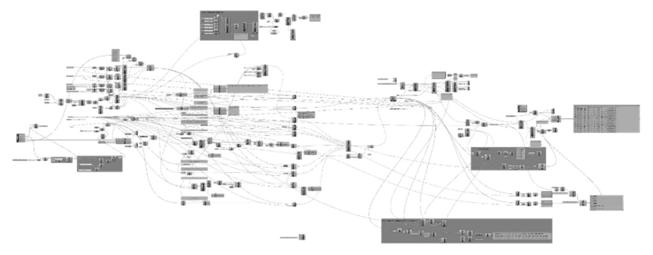
Figure 6.
Full Grasshopper3D definition to control rover-robot I/Os, milling points coordinates, trajectory planning and post-processing for the Doosan arm.
Figure 6.
Full Grasshopper3D definition to control rover-robot I/Os, milling points coordinates, trajectory planning and post-processing for the Doosan arm.
3. Methods
3.1. Fine-Tuning a Segmentation Model to Perform Defect Recognition
3.1.1. Introduction SAM Fine-Tuning
In this study, a pre-trained foundation model for promptable segmentation was fine-tuned to obtain a system capable of automatically segmenting visible superficial wood-knots identified as defects.
Among those currently available in the literature, the pre-trained Segment Anything Model (SAM), developed by Meta AI, was chosen for the study for image segmentation that can perform zero-shot generalization [18]. The main reason behind its selection is the dataset used for its training, i.e., SA-1B, the largest in existence, with more than 11 million images and 1.1 billion masks.
Despite its notable zero-shot performance, SAM exhibited limited accuracy in the segmentation of wood knots when using bounding box prompts. As demonstrated in the comparative segmentation results - replicable using the official SAM online demo [20] and illustrated in Figure 7 - the model consistently failed to delineate wood knots with sufficient precision. It frequently incorporated surrounding wood grain, cracks, and other unrelated textural elements, thereby compromising the specificity required for accurate defect identification.
To address these shortcomings, a fine-tuning phase was conducted. During this stage, the decoder parameters responsible for mask generation were updated using datasets focused on wood defects.
A key objective of the present research was to demonstrate the feasibility of fine-tuning a pre-trained computer vision model for accurate, task-specific segmentation using a limited dataset that a single annotator can independently produce.
3.1.2. Dataset Preparation for Fine-Tuning
The training datasets used in this study consisted of images of cut timber surfaces and their corresponding ground-truth masks — binary black-and-white images in which wood knots (considered as defects) are highlighted in white.
Four different datasets were employed during the fine-tuning phase to assess whether accurate segmentation of wood defects could be achieved without relying on large-scale datasets, which are often expensive and time-consuming to produce independently. The two base datasets were: Dataset 1, a publicly available dataset [21] comprising 20,276 images of wooden planks with corresponding segmentation masks; and Dataset 2, a manually curated dataset, independently acquired and annotated by a single researcher, consisting of 60 images of glulam beams with corresponding ground-truth masks.
During the dataset preparation phase, several filtering and preprocessing steps were performed. For Dataset 1, all images with either empty masks or masks that did not contain wood knots (e.g., masks indicating only cracks, mold stains, or resin pockets) were excluded. This filtering step was not necessary for Dataset 2, as it had been created specifically for the project and already included only relevant masks.
Subsequently, the images and their corresponding masks from both Dataset 1 and Dataset 2 were divided into 256×256-pixel patches. Patches with empty corresponding masks were discarded from further use. This preprocessing step resulted in a total of 6,760 patches (with masks) of 256×256 pixels derived from Dataset 1, and 642 patches (with masks) of the same size obtained from Dataset 2 (Figure 8).
Data augmentation techniques were then applied to Datasets 1 and 2. These included 90° rotations, mirroring, and random angle rotations; as a result of these augmentations, two additional datasets were generated, namely Dataset 3 and Dataset 4. Data augmentation was a necessary step to improve the generalization performance of the fine-tuned model. In the original datasets, the wood grain was consistently aligned vertically, introducing a strong directional bias. This could have led the model to overfit vertical grain patterns during training and perform poorly when encountering images with different grain orientations (e.g., horizontal or diagonal) during inference. The four datasets used in the fine-tuning phase were as follows [22]:
- Dataset 1: 6,760 patches (256×256 pixels)
- Dataset 2: 642 patches (256×256 pixels)
- Dataset 3: 53,117 patches (256×256 pixels) — augmentation of Dataset 1
- Dataset 4: 5,099 patches (256×256 pixels) — augmentation of Dataset 2
3.1.3. Fine-Tuning Process
The Segment Anything Model consists of three core components: a vision encoder, which extracts visual features from the input image; a prompt encoder, which encodes the input prompts (such as masks, bounding boxes, or points) and a mask decoder, which generates segmentation masks based on the encoded visual and prompt features. During fine-tuning, only the parameters of the mask decoder were updated, while those of the vision encoder and prompt encoder remained fixed. This approach preserved the feature extraction capabilities of the vision encoder, given its established generalization across a wide range of image-related tasks.
The Adam optimizer was employed to update the mask decoder weights. Optimization was performed using a composite Dice Cross-Entropy (Dice CE) loss function, which integrates both region-based (Dice) and pixel-wise (Cross-Entropy) loss components.
During fine-tuning, three hyperparameters were varied: the number of epochs, the learning rate, and the weight decay. Each dataset was randomly split into training and validation subsets, with 80% of the data used for training and 20% for validation. Model performance on the validation set was assessed using the F1 Score. The F1 Score was computed exclusively for the positive class, corresponding to the white pixels representing wood defects, without averaging with the F1 Score of the negative class (black pixels, i.e., background). This decision was motivated by the significant class imbalance in the binary masks, where the defect pixels were substantially underrepresented compared to the background. Averaging across both classes would have resulted in an artificial increase—approximately 15%—in the overall F1 Score, thereby reducing its relevance to the primary objective of accurately assessing defect segmentation performance. Additionally, Dice CE Loss was calculated during both training and validation to monitor potential overfitting. Results of the training phase consisted of seven checkpoints [22].
3.1.4. Dataset Preparation for Inference
Although the F1 Score was computed for each of the seven checkpoints during training, it is important to note that these evaluations were conducted on a validation set comprising 20% of the original dataset. As a result, there remained a substantial overlap in image characteristics, such as exposure, distortion, and resolution, between the training and validation sets, potentially biasing the evaluation. To more rigorously assess the generalization capability of the model checkpoints, two entirely new and independently acquired inference datasets, with distinct visual properties, were introduced to guide the final checkpoint selection. All data acquisition procedures were carried out by a single operator using a different camera (industrial smart camera Keyence IV4-G500CA) than that employed during the training phase. The image capture settings were systematically varied, including exposure times, flash activation, and camera-to-object distances. This was done deliberately to introduce heterogeneity in the dataset and thus assess the robustness of the segmentation models under diverse lighting and hardware configurations.
The inference datasets consisted of raw images of wooden glulam beams, resulting in two distinct sets: the Far_100 dataset, comprising 65 images captured at a distance of 100 cm from the target surface, and the Near_70 dataset, consisting of 65 images acquired at a distance of 70 cm to provide larger visual representations of the defects [22]. Since the two inference datasets contained original and unlabeled images, ground-truth masks were manually created for comparison and to enable the future calculation of the F1 Score metric (Figure 9).
3.1.5. Inference Pipeline Configuration
The segmentation performance of the fine-tuned model was evaluated by analyzing and comparing the behavior of the seven checkpoints across the two previously defined inference datasets. Each of the seven model variants was tested independently on both datasets, enabling the assessment of performance variation as a function of the distance between the imaging device and the wooden beam under inspection.
Preliminary tests revealed that the segmentation pipeline, in its default configuration, often failed to achieve optimal results. To address these limitations, an iterative parameter optimization procedure was implemented. This process targeted three key hyperparameters within the segmentation script: adaptive threshold, minimum size, and patch size. The adaptive threshold adjusts local thresholds to improve segmentation under varying lighting conditions. The minimum size filters out small noise or artifacts, improving accuracy without losing valid defects. Patch size of 512 × 512 pixels was selected for the Near_70 dataset, while a size of 256 × 256 pixels was adopted for Far_100. This choice was based on maintaining consistency between the knot-to-patch area ratio observed during training and that encountered during inference. When knots occupy disproportionately large regions within a patch, the model may fail to capture contextual boundaries, leading to inaccurate predictions.
It is essential to clarify that this procedure does not involve additional fine-tuning of the model weights. Instead, it represents an inference-level optimization in which segmentation parameters are adapted to the characteristics of real-world application data to enhance model output without retraining. All three parameters were systematically adjusted for each checkpoint, and the resulting masks were compared against the input images to evaluate segmentation accuracy. The next chart in Figure 3 describes the checkpoint parameters with the best segmentation performances.
3.1.6. Selection of Optimal Checkpoint
The seven checkpoints were evaluated during the inference phase on both test datasets, resulting in a total of 14 separate performance measurements, as illustrated in Figure 10. Among the checkpoints fine-tuned from the publicly available dataset, Checkpoint 1 exhibited the highest performance, achieving a mean F1 score of 0.353 with a standard error of ±0.021. In contrast, the best-performing model overall was Checkpoint 7, which had been fine-tuned on the custom dataset generated internally. This model achieved a mean F1 score of 0.686 (±0.019), and was consequently selected for integration into the Woodot system for subsequent deployment. A side-by-side comparison between Checkpoint 1 and Checkpoint 7 is presented in Figure 12 and Figure 13.
3.2. The five Woodot Subsystems
3.2.1. Rover Handling
In the first phase, for the rover to cruise the space, avoiding collisions, the work environment has to be pre-mapped to identify spatial constraints and include reference points for operations. The surroundings can also be explored on-the-fly, which is more practical in highly variable settings where the presence of obstacles may change frequently due to ongoing activities [9], but it was deemed unnecessary in this condition, with a predefined layout of the glulam beams and without any un-signaled workers crossing the scene.
Obstacle-avoidance and navigation on incoherent portions of the pavement are handled by generating dynamic point clouds to map the surroundings through the LiDAR sensor and complementing the virtual environment by employing stereo-camera vision sensors with 3D perception in order to detect objects, classify them, and determine their spatial position [9]. Once a work plan has been established, a vehicle’s mission can be defined in advance using ROS, setting common waypoints near each beam, including navigation parameters like the appropriate speed, the waypoint trajectory interpolation, and the main vehicle’s orientation when approaching objects. Navigation is then managed by planning algorithms that use pre-collected data, detailed work plan, and real-time obstacle detections to continuously control the vehicle’s movement, monitor its behavior, and correct any deviations from the expected path.
The first Docker service that was deployed is thus responsible for monitoring the state of the rover, continuously checking a digital input on the robot controller to begin communication with the robot arm.
When the rover is in a particular state, near the beam in correspondence to a predefined rover waypoint, this service opens a socket and streams a specific configuration to the robot arm. This configuration causes the end-effector of the robot arm to rotate, positioning the camera orthogonally to the selected portion of the beam surface.
3.2.2. Image Acquisition
At a fixed working distance of 1000 mm from the target surface, the Canon EOS 1200D equipped with a standard EF-S 18–55 mm lens is capable of capturing a field of view corresponding to approximately 0.47 m².
Its higher resolution, broader coverage, and adjustable optics make it more suitable for this particular task, involving variable acquisition conditions (especially in terms of the quality of the indoor lighting) and the possibility to manually change the camera focus to overcome image acquisition errors.
In fact, even if the dataset used for training the model had been created employing the Keyence IV4-G500CA smart camera, the lack of dynamic focusing capability, compounded by its significantly lower spatial resolution and narrower field of view, limits its effectiveness in applications requiring fine-grained visual detail and adaptable framing. Under identical distance conditions, the Keyence smart camera captures a significantly narrower field of view of 0.12 m², amounting to only 25% of the area covered by the Canon DSLR system.
This substantial difference is primarily attributed to the optical characteristics and sensor format of the two imaging systems. The Canon EOS 1200D, equipped with an APS-C CMOS sensor, offers considerable spatial detail, enabling flexible control over the image acquisition process. Conversely, the Keyence IV4-G500CA utilizes a CMOS sensor measuring approximately 0.876 centimeters. With a resolution of around 1.2 megapixels, integrated within a fixed-focus lens assembly designed for high-speed inline industrial inspection, without continuous autofocus capabilities during operation.
The second service, dedicated to camera streaming, employs the “gphoto2” [12] library to set up the Canon DSLR camera to acquire photos with selected shutter speed, aperture, and ISO settings. These images are then saved to a shared folder, accessible to the other services within the infrastructure.
The camera matrix for the DSLR has been calculated using a calibration process on a chessboard, captured from various angles and distances. Key feature points in the chessboard corners are spotted to serve as the basis for establishing the link between the real-world coordinates of the pattern and their 2D representations on the image. With this data, a camera calibration algorithm is used to optimize the intrinsic parameters of the camera by minimizing the re-projection error. The output is the intrinsic camera matrix, a 3x3 matrix encoding information of the focal lengths in the x and y directions, which is used to undistort the captured images.
Figure 14.
Close-up of the end effector rotation to perform camera acquisition.
3.2.3. Image Elaboration for Defect Identification
As the image analysis module of Woodot is based on a deep learning pipeline tailored for wood surface inspection employing SAM, the primary objective is the identification of knots through segmentation. This approach involves pixel-wise classification of images to distinguish defect regions from intact wood. As evaluated in the previous section, the F1 score achieved by checkpoint 7, equal to 0.69, demonstrated its superiority in the task of wood knot segmentation, thereby identifying it as the most suitable choice among the tested models.
The defect identification docker service scans the shared folder for the captured photos and employs the model to detect and draw bounding boxes around any identified defects. The centroid coordinates of these bounding boxes are then saved to a text file on the shared folder for the subsequent operation to be performed.
Figure 15.
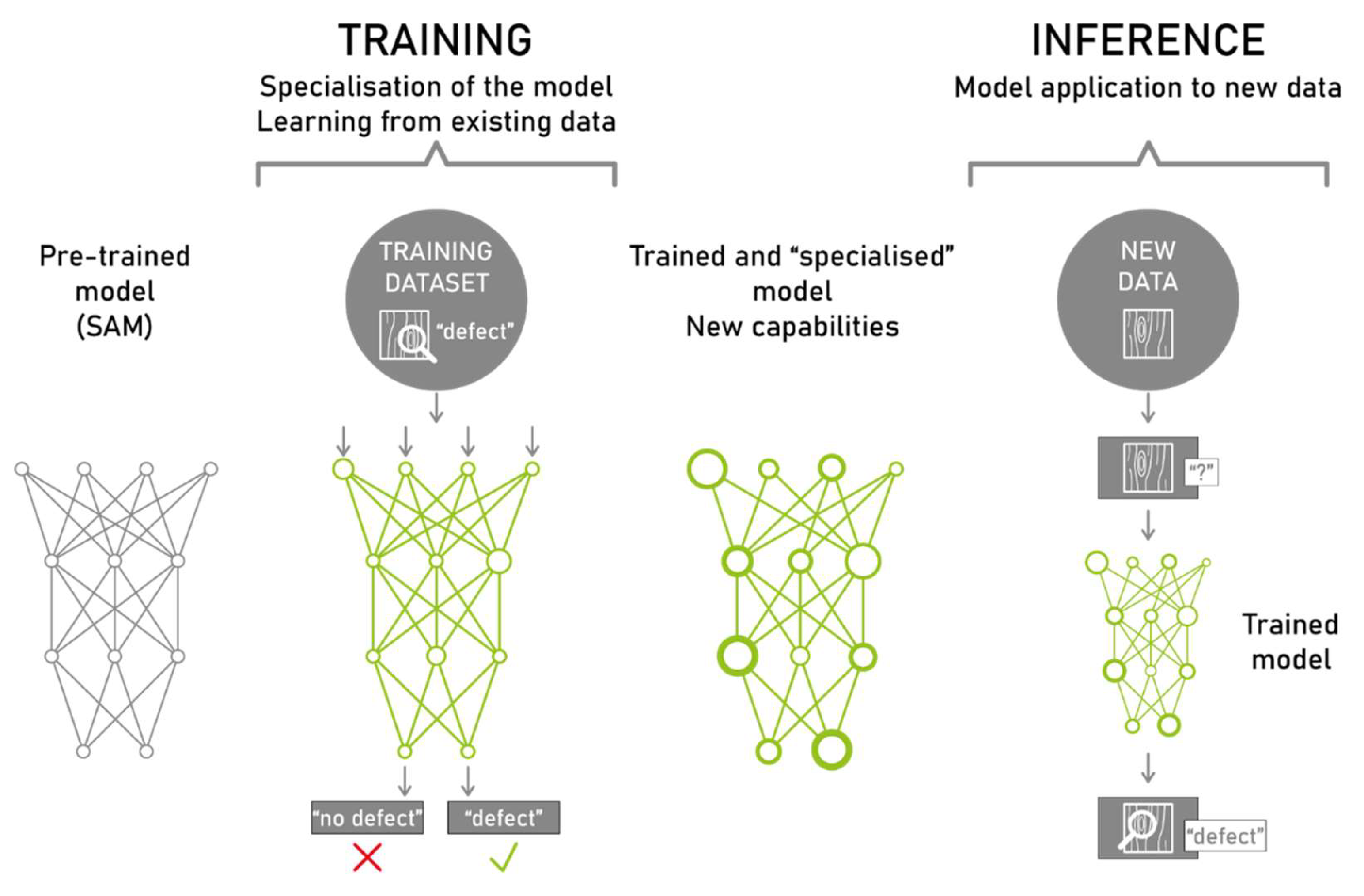
Custom training of the Woodot system enables re-use and further implementation of the dataset on new use-cases.
Figure 15.
Custom training of the Woodot system enables re-use and further implementation of the dataset on new use-cases.
3.2.4. Defect Removal
Another Docker service is responsible for streaming the milling trajectories to the Doosan robot. Similar to the first service, it opens a socket and transmits the necessary trajectories to the robot, allowing it to perform the required milling operations.
Before streaming, a Python script opens Grasshopper3D, and the real robot arm position and configuration are simulated. Every defect’s centroid corresponds to a certain wooden plug diameter coherent with the milling job settings. Within this simulation, the centroid coordinates from the segmentation process are ingested, and the script derives the necessary milling trajectories based on various parameters, such as the desired cutting speed, depth, and tool width.
The script generates a series of waypoints that the robot arm must follow to effectively mill the identified defects, while also ensuring that any potential collisions are avoided, and singularities are circumvented. The adherence to the surface of the beam is ensured by the impedance control of the collaborative robot, which is very useful for any milling, polishing, or grinding tasks where the robot needs to maintain a consistent contact force.
To simulate the behavior of the Doosan robot within the Grasshopper3D environment, the script utilizes Visose’s “Robots”[14] plugin, which provides a custom interface for simulating programs with robotic systems.
Finally, a custom post-processor - that was developed to translate geometric information from the Grasshopper3D simulation into the robot code required by the Doosan H2515 robot - enables the trajectory-streamer service to send milling instructions to the physical robot arm.
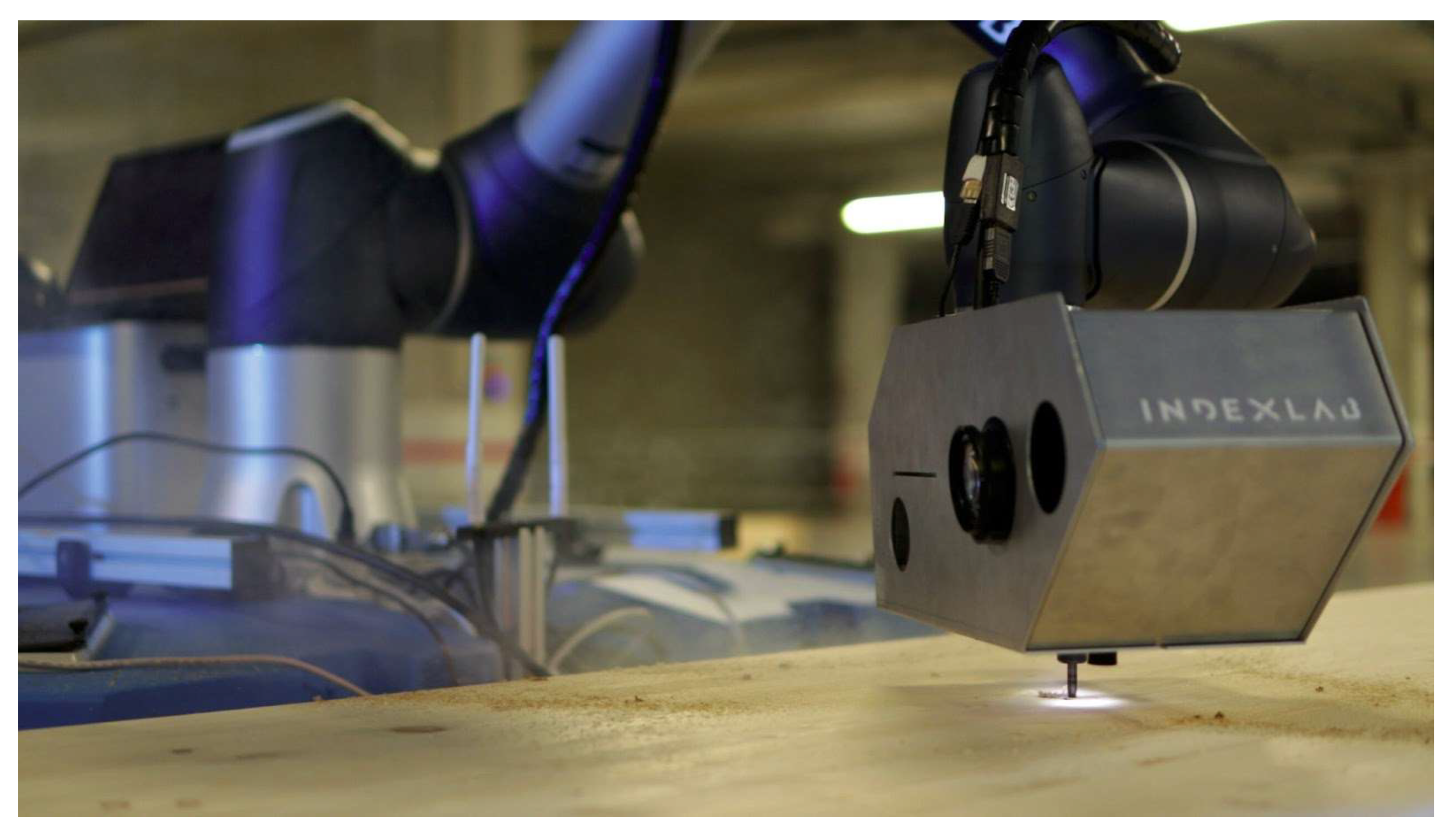
Figure 16.
Close-up of the end effector while milling the wood knot.
3.2.5. Insertion of Restoration Material
The final task is to turn the end-effector and place the plug in correspondence to the milled hole, and finally to signal the rover that the job is finished and to move to the next waypoint.
Wooden plugs are grouped in batches on the collaborative robot’s end-effector, where a manual pre-check is conducted before the insertion to ensure proper placement and alignment. Once the plugs are in place, the robotic arm moves to an approach point in correspondence with the milled hole on the surface.
A spiral search routine is thus kicked off, and the end-effector, rotated on the side of the plugs, wanders along a gradually widening spiral path, a method designed to locate the hole with precision.
As the arm searches the hole, its built-in collision control mechanism continuously monitors for any signs of contact. When the plug makes contact with the intended target, identified by a change in force feedback from the collision sensor, the system recognizes that the correct hole has been found. At that moment, the robot transitions from its search behavior to an insertion action, aligning itself accurately with the milled hole.
During insertion, the plug is gently pushed into the opening, with the collision control ensuring that the interaction is safe and that no excessive force is applied to either the plug or the surrounding structures. Once the insertion is complete, the arm moves in the Z direction and turns back to its home position on the rover, outputting a signal to go on to the next portion of the beam.
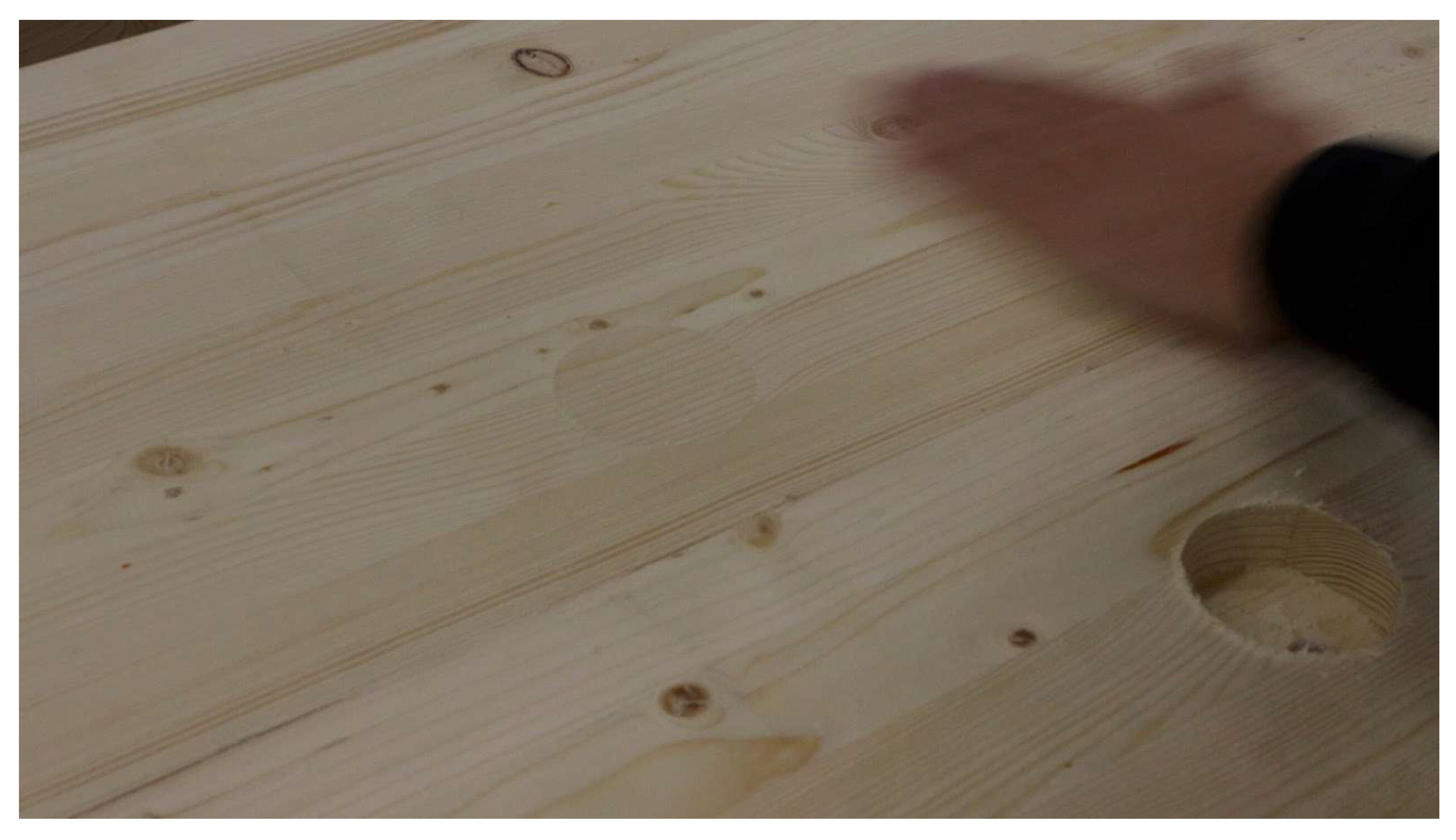
Figure 17.
Close-up of the restored surface of the wooden glulam beam.
4. Results
The performance of the Woodot system was evaluated by testing its complete autonomous workflow on real curved laminated timber beams. The results are presented according to the system’s key functional modules: navigation and positioning, defect identification accuracy, and restoration operation precision.
4.1. Navigation and Positioning Performance
Woodot’s rover demonstrated reliable autonomous navigation in unstructured environments, including cluttered workshop floors and variable lighting conditions. The integrated LiDAR sensors enabled safe maneuvering and obstacle avoidance. The robot consistently achieved positional tolerances within ±1 cm relative to the target beam location. Switching between global navigation and local alignment mode allowed the robot to precisely position the arm within the operational workspace of the beam, adapting to different geometries and beam curvatures.
4.2. Defect Identification Accuracy
Regarding the fine-tuning of the SAM segmentation model, the checkpoints derived from the autonomously generated dataset (checkpoints 4–7) consistently outperformed those obtained from the public dataset (checkpoints 1–3). Despite being ten times smaller in size, the autonomous dataset yielded checkpoints with a mean F1 score of 0.635, representing a 2.3× improvement over the public dataset checkpoints, which achieved a mean F1 score of 0.269. In addition to superior segmentation performance, fine-tuning on the autonomous dataset required approximately 40% less computational time and resources. These results demonstrate that reliance on large public datasets—often prohibitive in terms of time and resource requirements—is no longer necessary to achieve competitive segmentation performance. This study highlights the potential for developing and publishing lightweight, autonomous “micro-datasets,” thus broadening the applicability of segmentation models to image domains underrepresented in existing large-scale datasets.
The system successfully detected knots of varying size, shape, and wood grain contrast, with a false positive rate under 12% and a false negative rate under 15% in optimal lighting conditions. Defect localization precision was measured as the Euclidean distance between ground truth and predicted mask centroids, averaging 4.3 mm.
4.3. Restoration Workflow Effectiveness
Although the physical operations of plug insertion were manually validated for this iteration of the system, preliminary automated trials indicate high mechanical repeatability. The robotic arm followed pre-planned milling trajectories with a dimensional tolerance of ±0.5 mm in diameter and ±0.2 mm in depth. Plug insertion was tested on cylindrical wood inserts, and the success rate of flush placement without visual gaps was 87% in the first pass. The remaining cases were due to minor misalignment in tool calibration, which will be addressed in the next development phase.
4.4. Operational Cycle Time
A full knot remediation cycle (detection, classification, milling, and plug insertion) took an average of 74 seconds per defect. This includes all inter-module communication and repositioning time. Compared to traditional manual operations, which typically range from 3 to 5 minutes per knot depending on beam complexity, Woodot’s process offers a time reduction of over 60%, with a significant improvement in repeatability and reduced operator fatigue.
These results validate the effectiveness of Woodot as a mobile robotic system for autonomous visual quality control and aesthetic restoration of curved laminated beams. Further refinements in calibration, tool handling, and model robustness are expected to enhance performance in real production environments.
5. Discussion
The implementation and testing of the Woodot system reveal both the opportunities and the challenges associated with deploying intelligent mobile robotics in the domain of curved glulam beam processing. From a technological perspective, Woodot combines mobility, perception, and manipulation into a unified platform capable of autonomously identifying and repairing wood knot defects. This integration allows for intervention in environments where traditional linear automation systems are ineffective or impractical.
Compared to static robotic cells or CNC-based defect handling, Woodot’s mobility enables it to service non-standard and geometrically complex timber components without predefined positioning, making it uniquely suited for dynamic workshop conditions. The deployment of AI-driven segmentation significantly enhances defect detection accuracy and adaptiveness, as demonstrated by the quantitative performance of the trained SAM-based model. In particular, the use of a small but application-specific dataset yielded higher F1 scores than larger generic datasets, reinforcing the value of tailored data in industrial AI applications. From an operational standpoint, Woodot demonstrated significant time efficiency compared to manual remediation of knots, offering consistent results with lower physical and cognitive workload for human workers. While the mechanical performance of the milling and plugging modules still requires fine-tuning for full automation, the current system already enables a semi-autonomous workflow with clear productivity and quality advantages.
Nevertheless, some limitations remain. These include the dependency on stable lighting conditions for optimal vision performance and the need for tool calibration checks.
Future development will focus on improving tool-changer reliability, expanding the plug insertion toolkit, and introducing online retraining capabilities to enhance model robustness across timber species and surface finishes. Additionally, the efficient containerization using Docker enables a more optimal use of resources in the future. By packaging applications and dependencies, Docker allows for seamless deployment to any cloud-based infrastructure, with the possibility of using an orchestration platform like Kubernetes to manage and scale containers as needed across a cluster of machines, ensuring high availability, scalability, and efficiency.Setting up a “Rhino.Compute”[16] service to call a cloud-based server, it would be possible to offload computationally intensive tasks to the cloud, thereby enhancing processing efficiency and reducing the local workload on the host machine. Multiple requests can be called concurrently, deploying Rhino.Compute in a production environment, such as a Windows-based VM or a headless server, monitoring the performance and optimizing it as needed to ensure efficient use of resources and minimize cycle time and computational costs. These developments will significantly reduce the load of computing image segmentation and robot path-planning on the host machine.
Woodot introduces a novel paradigm in timber defect remediation, effectively bridging adaptive robotics with the practical constraints of workshop-level production. Its architecture and results provide a foundation for further research and industrial application in wood construction automation.
Supplementary Materials
All source code, trained weights, and raw datasets are openly available at Zenodo repository under the accession number 10.5281/zenodo.15304349, and it is publicly available at: https://doi.org/10.5281/zenodo.15304349. A video of Woodot can be found at https://www.indexlab.it/woodot . Other data that support the findings of this study are available on request from the corresponding author.
Author Contributions
The authors of this paper thank their colleagues at Indexlab — Carlo Beltracchi, Imane El Bakkali, Gabriele Viscardi, Zahra Cheragh Nia, Carolina Moroni, Filippo Bianchi —who contributed to the technical development of the system.
Funding
This research is auto financed by the authors and the companies involved. No-conflicts with third parties.
Acknowledgments
The authors of this paper thank the companies Sigma Ingegneria, Homberger, Eurostratex, that supported the research, and in particular Simone Giusti, Matteo Pacini, Beatrice Greta Pompei, Elisabetta Pisano, Giovanni De Santa, Roberto Ancona, Matteo Bardelli , Gianni Ossola; The authors would also like to express their heartfelt gratitude to Senaf for promoting innovation in the context of SAIE, and specifically, the authors thank Emilio Bianchi, Tommaso Sironi, Elisa Grigolli, Michele Ottomanelli, Andrea Querzè.
Conflicts of Interest
The authors declare no conflicts of interest.
References
- Hashim, U.R.; Hashim, S.Z.M.; Muda, A. Automated vision inspection of timber surface defect: A review. Jurnal Teknologi 2015, 77, 1–10. [Google Scholar] [CrossRef]
- Biederman, M. Robotic Machining Fundamentals for Casting Defect Removal. M.S. Thesis, Oregon State University, OR, USA, 2016. [Google Scholar]
- Li, R.; Zhong, S.; Yang, X. Wood Panel Defect Detection Based on Improved YOLOv8n. BioResources 2025, 20, 2556–2573. [Google Scholar] [CrossRef]
- Andersson, P. Automated Surface Inspection of Cross Laminated Timber. Master’s Thesis, University West, Sweden, 2020. [Google Scholar]
- Nagata, F.; Kusumoto, Y.; Fujimoto, Y.; Watanabe, K. Robotic sanding system for new designed furniture with free-formed surface. Robotics Comput. Integr. Manuf. 2007, 23, 371–379. [Google Scholar] [CrossRef]
- Timber Products Company. Robots Introduced to Grants Pass – Automated Panel Repair Line. Available online: https://timberproducts.com/robots-introduced-to-grants-pass/ (accessed on 19 April 2025).
- Toman, R.; Rogala, T.; Synaszko, P.; Katunin, A. Robotized Mobile Platform for Non-Destructive Inspection of Aircraft Structures. Applied Sciences 2024, 14, 10148. [Google Scholar] [CrossRef]
- Sigma Ingegneria. Il sistema Woodot per l’edilizia del futuro: un rover con braccio robotico per le travi lamellari. Blog Sigma – SAIE 2024 Preview, 26 Sept 2024.
- Ruttico, P.; Pacini, M.; Beltracchi, C. BRIX: An autonomous system for brick wall construction. Constr. Robot. 2024, 8, 10. [Google Scholar] [CrossRef]
- Patil, S. , Vasu, V. & Srinadh, K.V.S. Advances and perspectives in collaborative robotics: a review of key technologies and emerging trends. Discov Mechanical Engineering 2, 13 (2023). [CrossRef]
- Faccio, M. , Granata, I., Menini, A. et al. Human factors in cobot era: a review of modern production systems features. J Intell Manuf 34, 85–106 (2023). [CrossRef]
- gphoto.org. gPhoto Website. Available online: http://gphoto.org/ (accessed on 20 August 2024).
- Meta AI. Segment Anything GitHub Repository. Available online: https://github.com/facebookresearch/segment-anything (accessed on 20 August 2024).
- visose. Robots GitHub Repository. Available online: https://github.com/visose/Robots (accessed on 20 August 2024).
- Robert McNeel & Associates. Grasshopper3D. Available online: https://www.grasshopper3d.com/ (accessed on 20 August 2024).
- Robert McNeel & Associates. Rhino3D Compute Developer Guide. Available online: https://developer.rhino3d.com/guides/compute/.
- Available online: https://www.dewalt.co.uk/product/d26200-gb/8mm-14-fixed-base-router (accessed on 20 August 2024).
- IndexLab. Available online: https://www.indexlab.it/woodot (accessed on 20 August 2024).
- Kirillov, E. Mintun, N. Ravi, H. Mao, C. Rolland, L. Gustafson, T. Xiao, S. Whitehead, A. C. Berg, W.-Y. Lo, P. Dollár and R. Girshick, “Segment Anything,” arXiv preprint arXiv:2304.02643, 2023. [CrossRef]
- Meta AI, “Introducing Segment Anything: Working toward the first foundation model for image segmentation”, Meta AI Blog, 2023. Available online: https://ai.meta.com/blog/segment-anything-foundation-model-image-segmentation/.
- Kodytek, P.; Bodzas, A.; Bilik, P. A large-scale image dataset of wood surface defects for automated vision-based quality control processes. F1000Research 2022, 10, 581. [Google Scholar] [CrossRef] [PubMed]
- Deval, M. , Bianchi, F., & Moroni, C. (2025). Wood knots defects dataset [Data set]. Zenodo. [CrossRef]
Figure 1.
The Woodot system displayed at the SAIE Fair in Bologna on October 9, 2024.
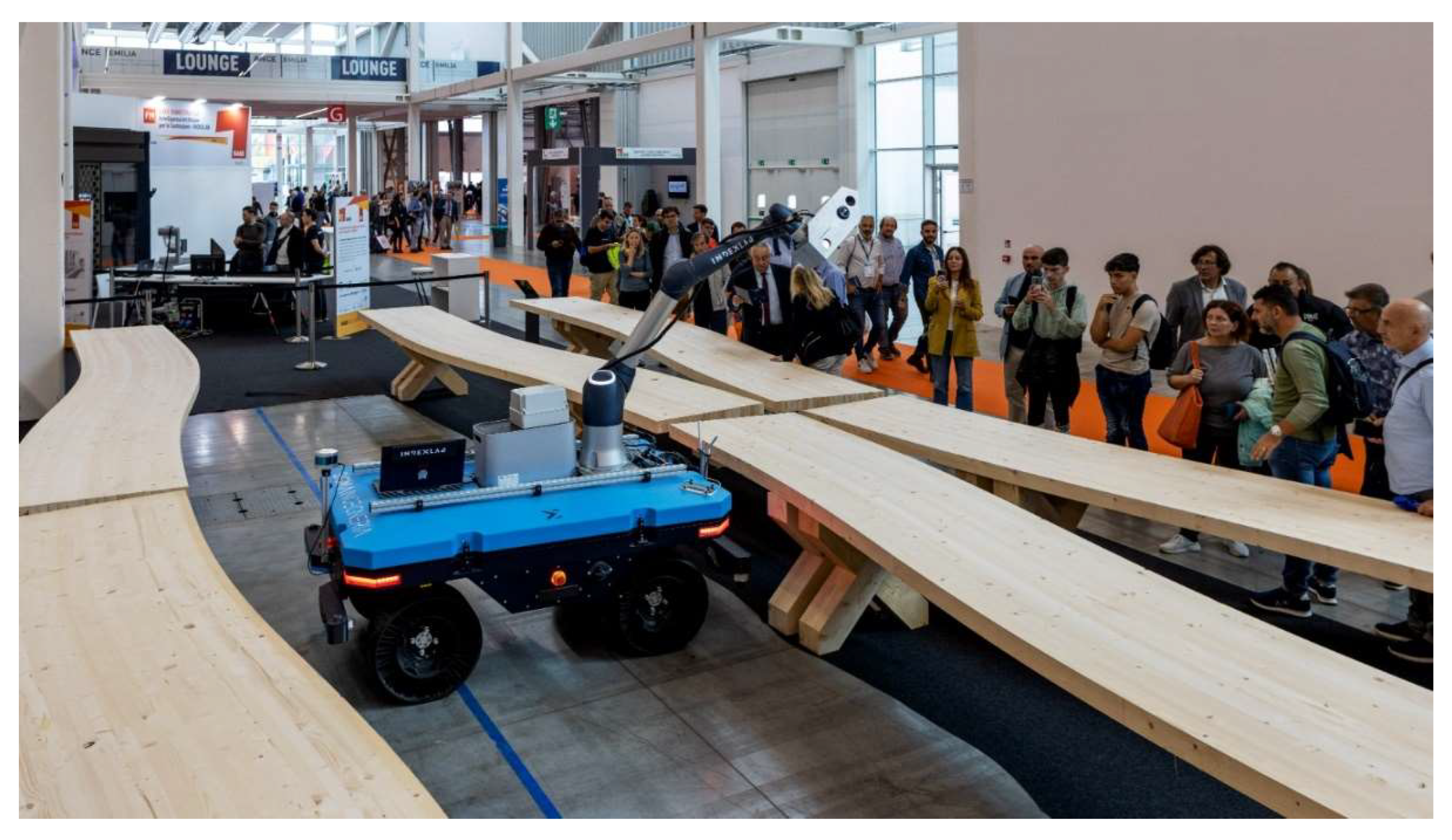
Figure 2.
Proof of concept of the milling phase of the Woodot system performed at INDEXLAB.
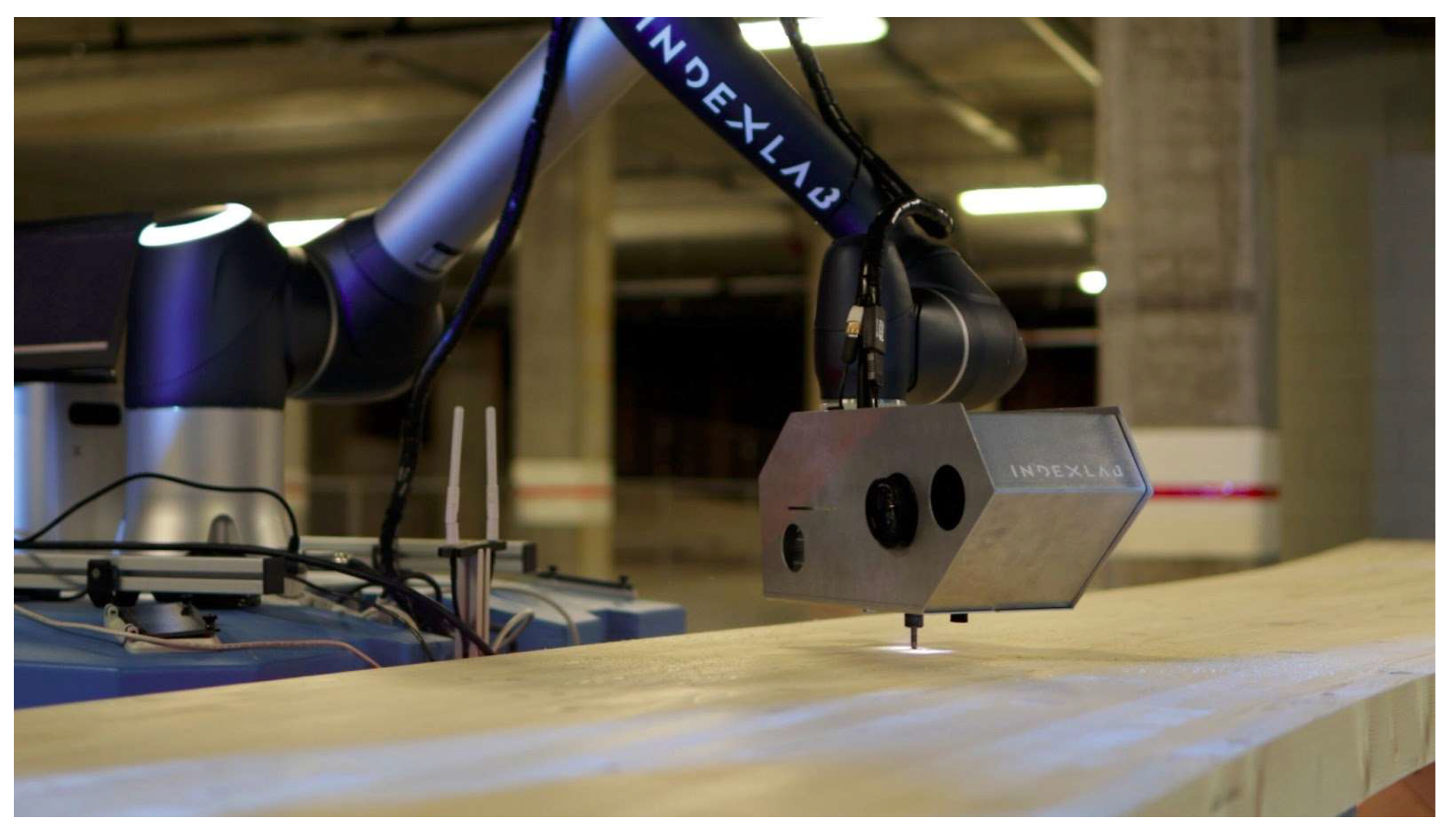
Figure 7.
From the left - original image - mask prediction with “everything” function - mask prediction with bounding box corresponding to the size of the image - mask prediction with bounding box corresponding to a specific wood knot.
Figure 7.
From the left - original image - mask prediction with “everything” function - mask prediction with bounding box corresponding to the size of the image - mask prediction with bounding box corresponding to a specific wood knot.
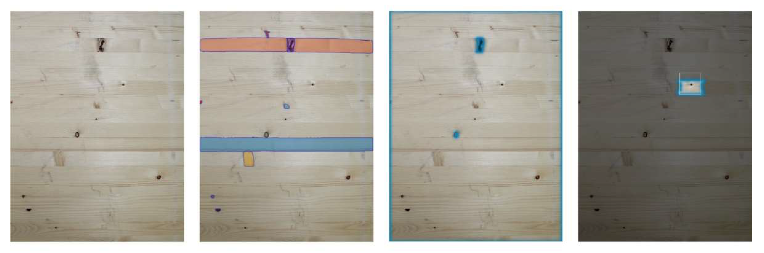
Figure 8.
From the left - Dataset 1 patch, Dataset 1 patch mask, Dataset 2 patch, Dataset 2 patch mask.
Figure 8.
From the left - Dataset 1 patch, Dataset 1 patch mask, Dataset 2 patch, Dataset 2 patch mask.
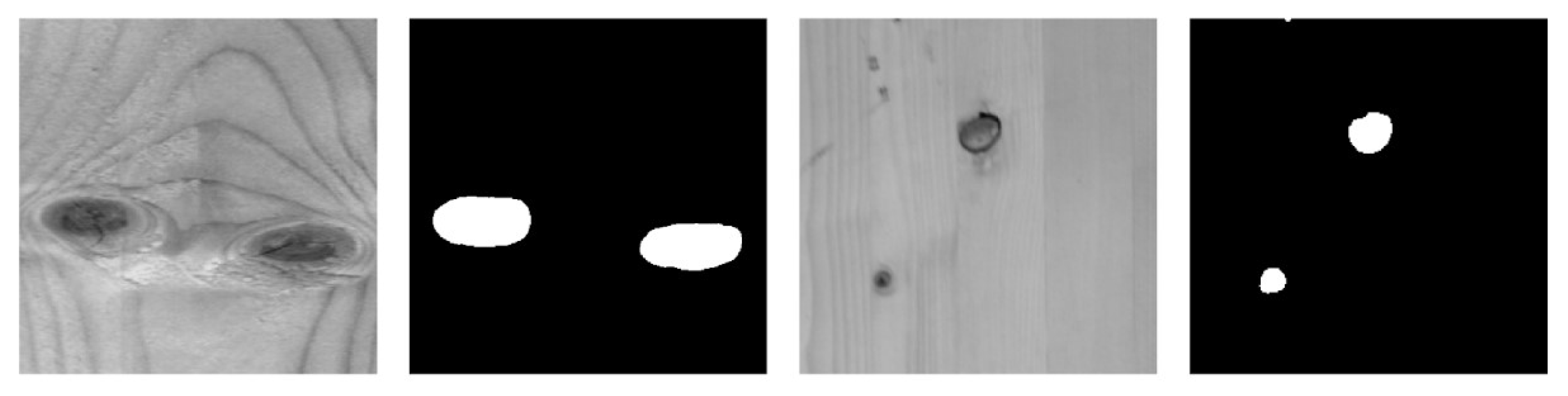
Figure 9.
From the left - Far_100 image, Far_100 mask, Near_70 image, Near_70 mask.
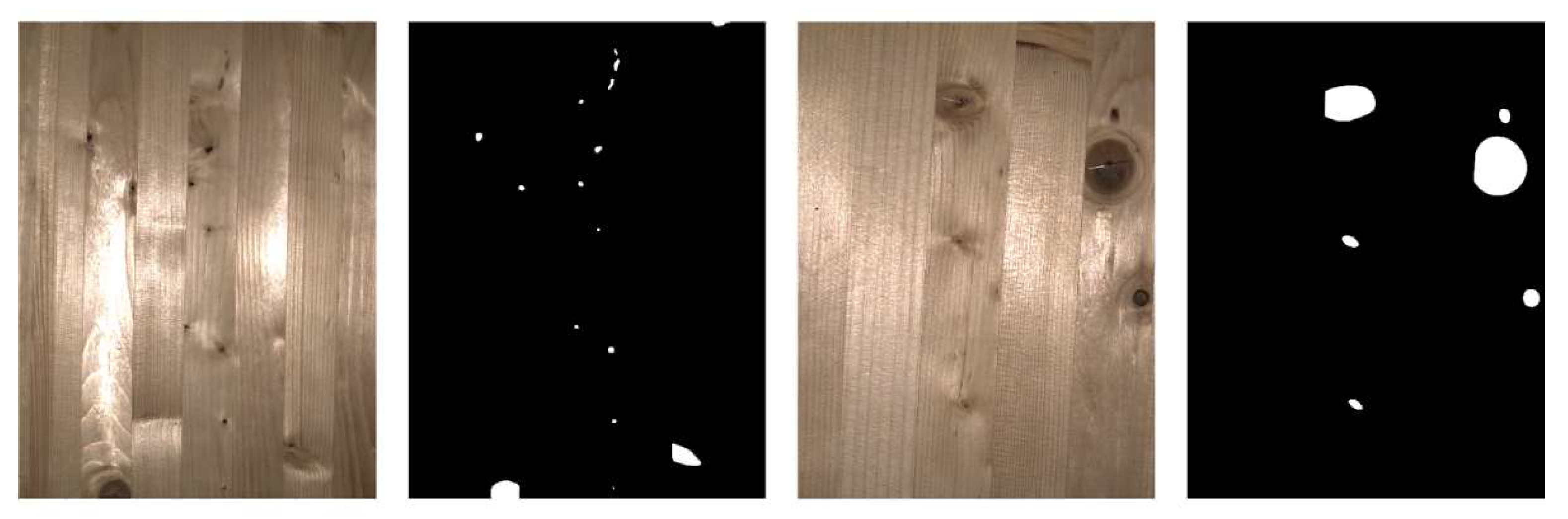
Figure 10.
Summary of the inference process with hyperparameters and results.
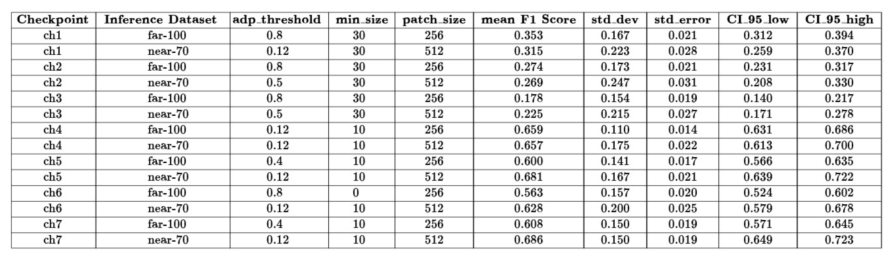
Figure 11.
Mean F1 Score of the 7 checkpoints based on the two inference datasets.
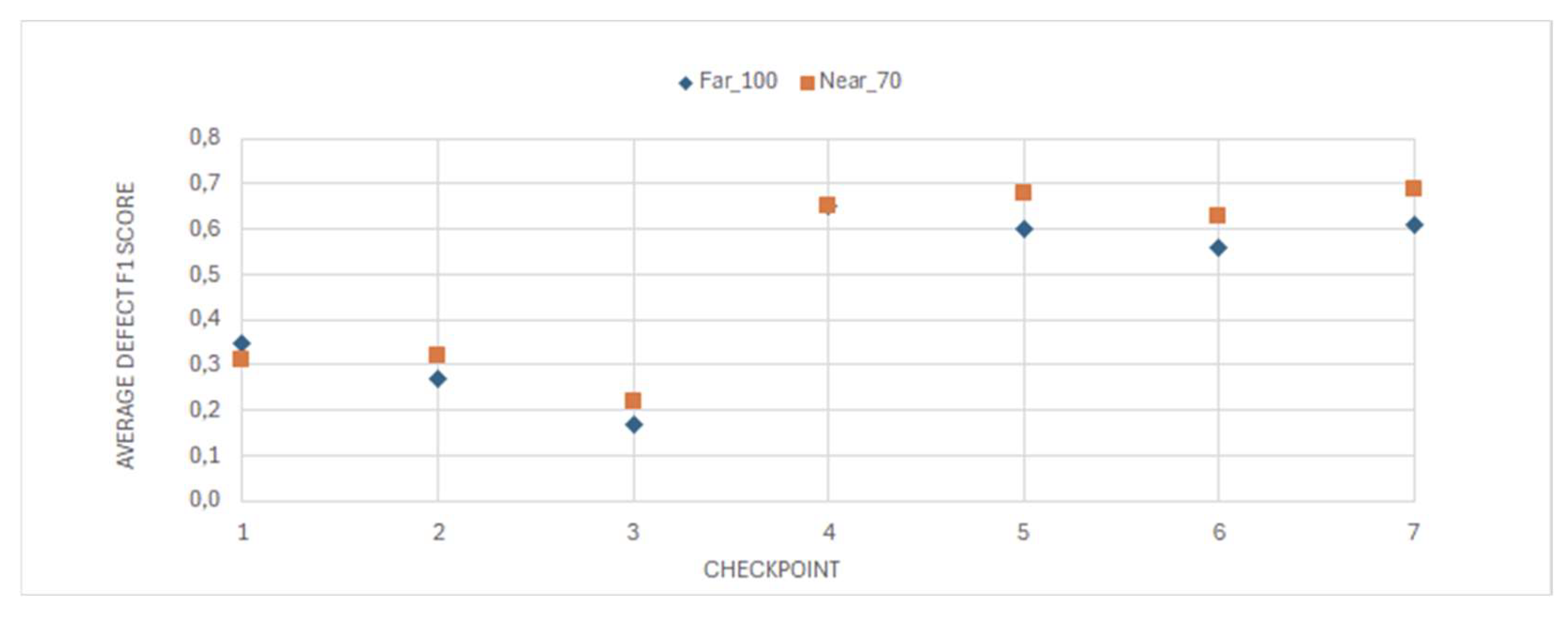
Figure 12.
From the left - original image, ground truth mask, mask prediction by ch1-far_100 (F1 score = 0.353) and mask prediction by ch7-far_100 (F1 score = 0.608).
Figure 12.
From the left - original image, ground truth mask, mask prediction by ch1-far_100 (F1 score = 0.353) and mask prediction by ch7-far_100 (F1 score = 0.608).
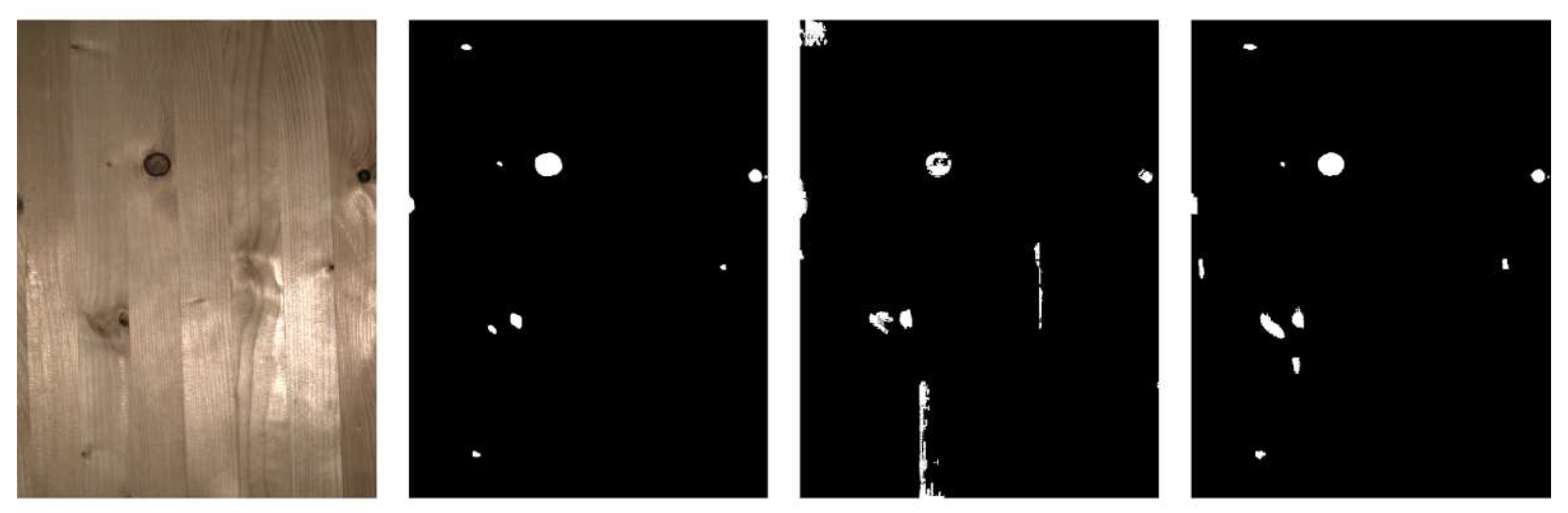
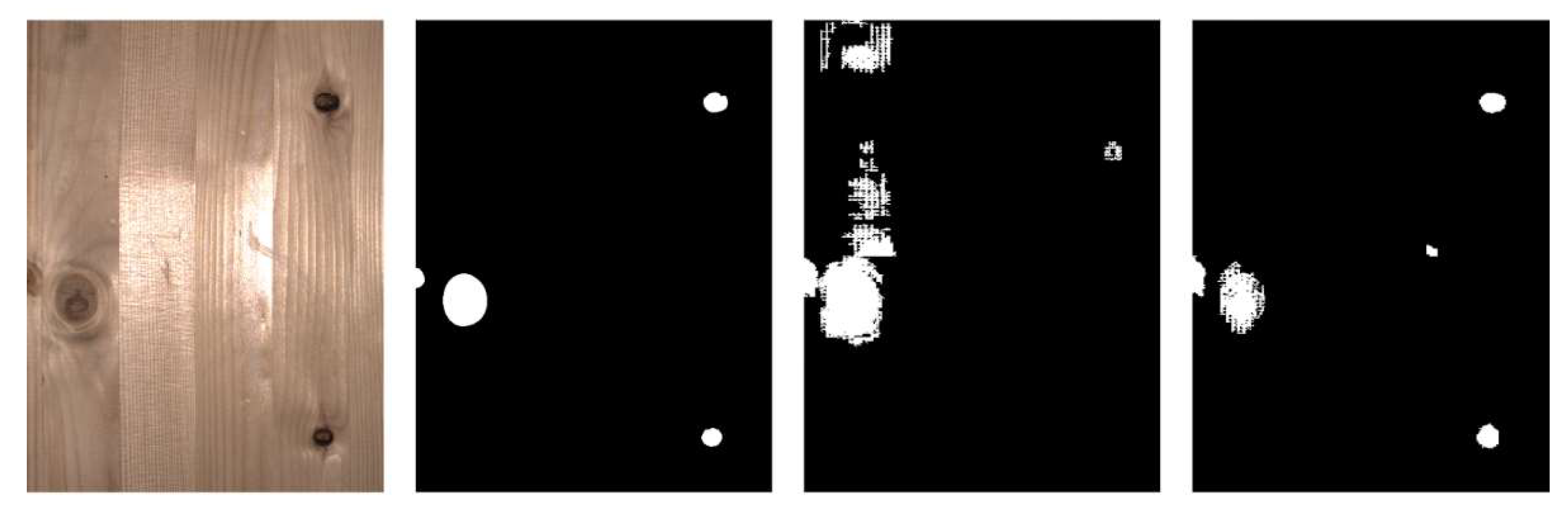
Figure 13.
From the left - original image, ground truth mask, mask prediction by ch1-near_70 (F1 score = 0.315) and mask prediction by ch7-near_70 (F1 score = 0.686).
Figure 13.
From the left - original image, ground truth mask, mask prediction by ch1-near_70 (F1 score = 0.315) and mask prediction by ch7-near_70 (F1 score = 0.686).
Disclaimer/Publisher’s Note: The statements, opinions and data contained in all publications are solely those of the individual author(s) and contributor(s) and not of MDPI and/or the editor(s). MDPI and/or the editor(s) disclaim responsibility for any injury to people or property resulting from any ideas, methods, instructions or products referred to in the content. |
© 2025 by the authors. Licensee MDPI, Basel, Switzerland. This article is an open access article distributed under the terms and conditions of the Creative Commons Attribution (CC BY) license (http://creativecommons.org/licenses/by/4.0/).
Copyright: This open access article is published under a Creative Commons CC BY 4.0 license, which permit the free download, distribution, and reuse, provided that the author and preprint are cited in any reuse.


