Submitted:
03 May 2025
Posted:
06 May 2025
Read the latest preprint version here
Abstract
Since the year 2001 and after decades of steady Magnitude ≥ 3 earthquake rate in the United States, the number of annual earthquakes have been increasing, deviating to up to 188 events in 2011. This is suspected to be human-induced. Although historical understanding of earthquakes have roots in classical mechanics and relatively slow motion of classical systems (e.g. plate tectonics), modern tools of physics such as statistical mechanics and complexity can shed light on processes which trigger seismicity, anthropogenic and otherwise. In this study, after introducing the methods of analysis, I have particularly examined anthropogenic processes such as wastewater and CO2 injections which can trigger seismicity. The San Andreas Fault (SAF) and the lake-fillings nearby (Salton Sea) is chosen as a complex system of interest. Bayesian Hypothesis testing is used to better understand fault behaviors. As a case study, the SAF single-fault model with RMSE of 1.4 was improved to a two-fault model with RMSE of 1. Furthermore, anthropogenic effects on SAF itself are examined using tools of complexity.
Keywords:
Bayesian
; Geophysical Data Analysis
; Seismicity
; Data Assimilation
; Anthropogenic Seismicity
; Complex Systems
1. Introduction
Geophysicists do not yet understand the exact physical processes that cause earthquakes and this is evident in the fact that earthquakes often come as a surprise. Deformation of Earth’s crusts which translate into earthquakes involve many-body problems and hence the emergence of a complex system. As an alternative approach to earthquake mechanics, Turcotte and Malamud have proposed that the tools of complexity rooted in statistical physics are capable of describing faults as a self-organizing complex system [1].
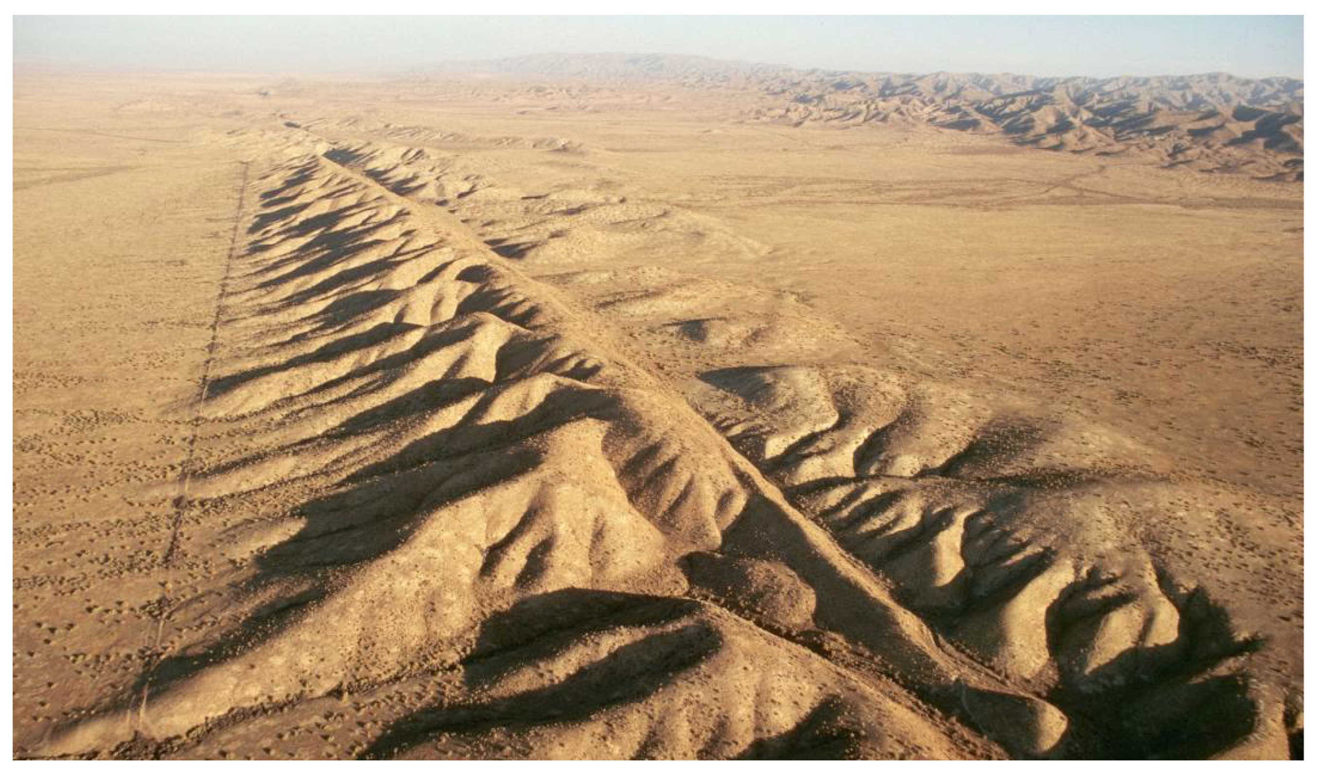
The San Andreas Fault is an example of such complex system in seismology, extending about 750 miles across central California (Figure 2.) Radiocarbon dating methods performed on this fault reveal the history of at least 10 episodes of large earthquakes on average every 132 years, ranging from the year 671 to January 9 1857 (with an estimated magnitude of 8.25) [2]. The absence of large earthquake episodes since, is explained using the theory that the fault-zone material do not heal after each de-formation and they lack strength needed to cause more destructive movements [3].
Tectonic faults behavior analysis is the central problem to geophysics and seismology [4,5,6] and therefore probabilistic hazard assessments require data assimilation and careful geophysical data analysis, which extend beyond the tools of complexity alone. Modern computational approaches to address fault analysis, such as Monte Carlo Markov Chain and Bayesian Inference are also rooted in statistical physics. In this study, these tools will be used to analyze fault behaviors in the presence of external factors such as hydrologic loads and anthropogenic activities (ranging from wastewater disposal to CO2 induced seismicity, which are known to trigger earthquakes [7], in an attempt to guide better policy recommendations.
1.1. The Carbonate-Silicate Cycle
1.1.1. Earth
Walker et. al. in 1981 argued that the atmospheric CO2 level on earth is controlled by the carbonate–silicate geochemical cycle [8] over geological timescales (Gyr). On a shorter timescale (yrs 1959-2020), the increasing CO2 trend is shown in Figure 1. Silicate weathering also impacts the Earth’s climate and carbon cycle [9], which is a key process for removing anthropogenic fossil fuel emissions over the next 10-100 Kyr in the absence of any human interventions [10,11,12,13].
1.1.2. Mars
On Mars, however, these cycles are not as well understood, given fewer experimental verifications which would require space missions for the purpose of Mars explorations (in the footsteps of NASA’s Mariner 9 and Viking Missions). Nevertheless, the carbonate-silicate cycle (by a () greenhouse gas is proposed to be the primary mechanism of Mars warming, with each cycle lasting up to 10 Myr, followed by extended periods of glaciation [18].
2. Bayesian Inference: The San Andreas Fault
Markov chain Monte Carlo (MCMC) has been widely used in Earth and Environmental sciences [19,20,21,22] and even in Cosmology and Materials Science [23,24,25]. Liu et. al. [26] have also shown that Bayesian inference can be used in inverse modeling of contaminants and air quality modeling and they used Bayesian analysis for Inverse modeling for Chernobyl and Fukushima Daiichi accidental releases of radionuclide. This author will use Bayesian Inference and MCMC to determine fault parameters from geophysical data, given a geophysical model, improving our understanding of fault mechanisms which lead to seismicity (for instance to study the relative motion of the American and Pacific plates across the San Andreas fault system, as shown in Figure 2). Next, the model will be validated against the collected data and the corresponding RMSEs for each model will be calculated.
Figure 2.
n aerial view of the San Andreas Fault System in Central California. It extends roughly 750 miles. Photo: [27].
Figure 2.
n aerial view of the San Andreas Fault System in Central California. It extends roughly 750 miles. Photo: [27].
2.1. The Inverse Problem: Why MCMC?
An inverse problem in science is the process (or processes) of calculating from a set of observations the causal factor(s) that produce(s) those observations [28].
That is to arrive at model parameters (The M Matrix), given data (The d Matrix). The complexity of this task increases with the model complexity and uncertainty. Meaning regular fitting methods would fail to produce satisfactory model parameters. Also, simple fittings do not use prior knowledge 1 whereas MCMC as a tool in Bayesian Inference updates beliefs about model parameters based on data [28,29].
It is noteworthy that unlike the frequentist approaches that take errors as a flaw in measurements, the Bayesian approach sees error as a feature and not a flaw. This touches on the fundamental philosophy behind using such approaches in applications such as data assimilation.
2.2. Single Fault Model
The velocity function describing fault slip is given by [30]:
Where is the fault slip rate, D is the locking depth, is the fault location, and x is the spatial coordinate.
The validity of this model when applied to the San Andreas fualt, will be examined using Bayesian Inference and will be compared to the values reported in the literature. However, it is noteworthy that to date, there are several theories about whether this fault might pose risks of larger earthquakes to the surrounding areas. Smaller earthquakes experienced are explained using the theory that the fault-zone material do not heal after each deformation and they lack strength needed to cause more destructive movements [3].
2.3. Data
The creep rate GPS and InSAR data [31] is plotted and shown in Figure 3. It is noteworthy that the creep rate peaks between , and a maximum of (mm/year) appears at . For a better visualization of the creep rate, it is plotted against latitude and is shown in Figure 4.
The Line Of Sight (LOS) velocity data [32] is assumed to have a variance of 1.
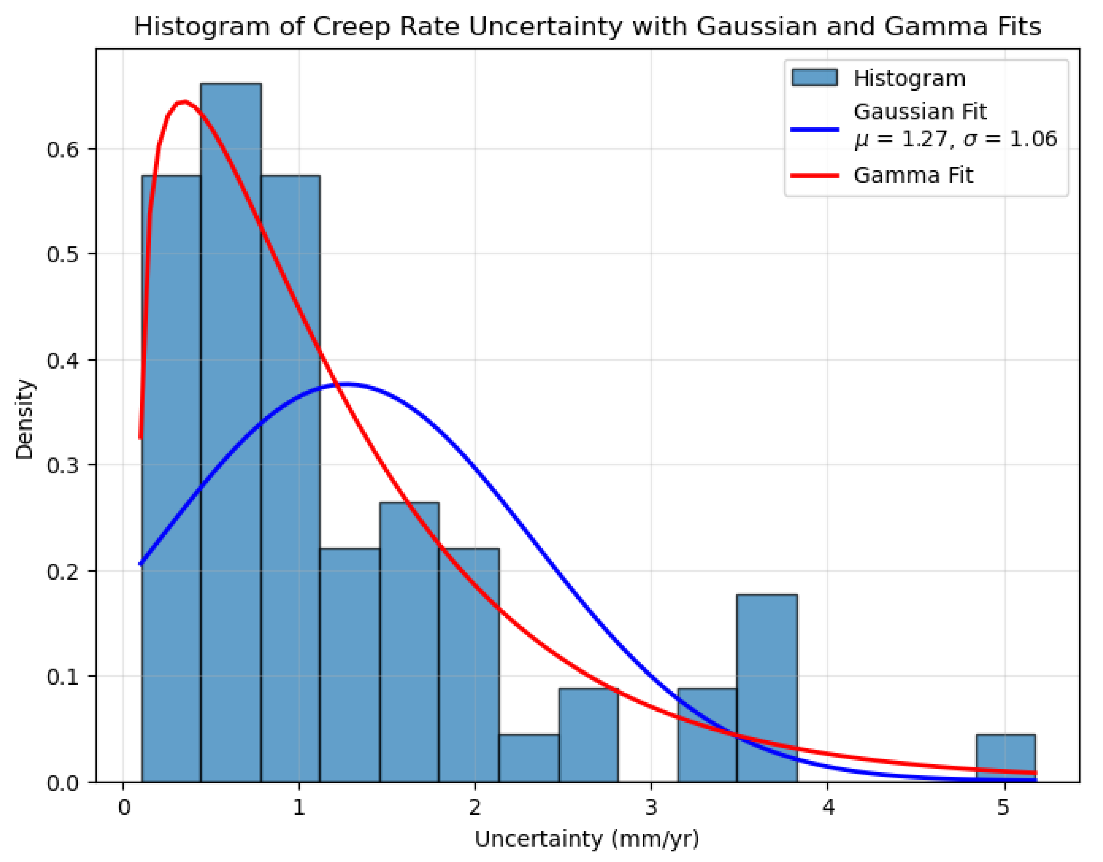
Creep rate uncertainty as suggested in [31] is 1.2 ± 1 (mm/year). The distribution of this uncertainty in measurement of the creep rate is shown in Figure 5. The data is loaded from a file (available in the GitHub repository for this project), assuming a two column structure separated by commas. First column is assumed to be the x(positions) and the second is the velocities . We also assume the the observational errors follow a Normal distribution, Where and STD with respect to the model equation given in eq. 3.
Figure 5.
Creep rate uncertainty distribution plotted for San Andreas fault based on high resolution GPS and InSAR data from Ref. [31]. The Gaussian fit shows a of 1.27, however, given the existence of heavy tails, a Gamma fit might be a better choice to fit the uncertainty data than just using a normal distribution. Gaussian peaks around 1.27 while Gamma peaks around 0.5. In Gamma fits, the average doesn’t represent the data.
2.4. Defining Log-Likelihood and Log-Prior
We want to know how well the model fits the data.
When taking the Log-Likelihhood, the product becomes a sum. Given , it simplifies to
Where A is a constant throughout the MCMC process.
2.5. Bayesian Context
In Bayesian Context, the Posterior distribution of the parameters given the data , which is our goal, is given as:
is the likelihood (How probable the observed data is under specific parameter values). is our initial beliefs about the parameters. is the Evidence, which is a normalizing constant, which can be ignored in MCMC since we are sampling ratios. So in order to find the posterior, we need to compute the likelihood, which determines how well a given set of parameters explains the data y.
2.6. Log-Prior, Single Fault
We have a uniform prior, where is a constant if within bounds, and if not, zero. So log prior would be 0 if valid and if not. The purpose of this is to constrain parameter ranges. For instance, and D both range between 0 and 80 while ranges from -50 to 50.
2.7. Random Walk Metropolis Sampler : Markov Chain Monte Carlo (MCMC)
This algorithm implements the Metropolis-Hastings MCMC algorithm. Starting at an initial guess, we propose a new point with S being the step scale. We then compute the log-posterior by taking the log of eq. 7, we arrive at:
The outputs are chain of samples, log-posterior values and acceptance rate.
2.8. Applying MCMC: Single Fault Model Analysis
The mean and STD of , D, are our posterior stats. The posterior distribution and correlations are plotted in Figure 6.
The MCMC model run over 30,000 samples burn-in of 5,000, step size 1.0:
2.9. Posterior Samples VS Data
Plot of the posterior samples vs Data is shown in Figure 8.
2.10. RMSE and the Two-Fault Model
The RMSE is defined as
where are the observations of the velocity, are the standard deviations of the model errors and is the velocity at location , using parameters . The RMSE for single-fault model is approximately . This is not disastrous, but not ideal either. To improve this, we consider a modified version of this model, namely "Two-Fault" model and see if we can arrive at a better RMSE.
2.11. The Two-Fault Model
In this model, instead of one fault, we consider two faults. We start by two-fault velocity, generalizing equation 3. , arriving at
The MCMC analysis is similar to that of single-fault model. The Two Fault Model Parameters are calculated and shown in Table 1.
It is noteworthy that there is a negative correlation between the two velocities and and these are exclusively shown in Figure 7.
For model validation, posterior samples are directly compared to experimental data. The error bars are not graphically displayed since they are relatively small and the points in Figure 8 overlap in representing the data and the corresponding uncertainty.
Figure 8.
Posterior Samples VS Experimental Data for the geophysical single-fault model. The model fits well, but it is not ideal, given a relatively large RMSE of 1.4.
Figure 8.
Posterior Samples VS Experimental Data for the geophysical single-fault model. The model fits well, but it is not ideal, given a relatively large RMSE of 1.4.
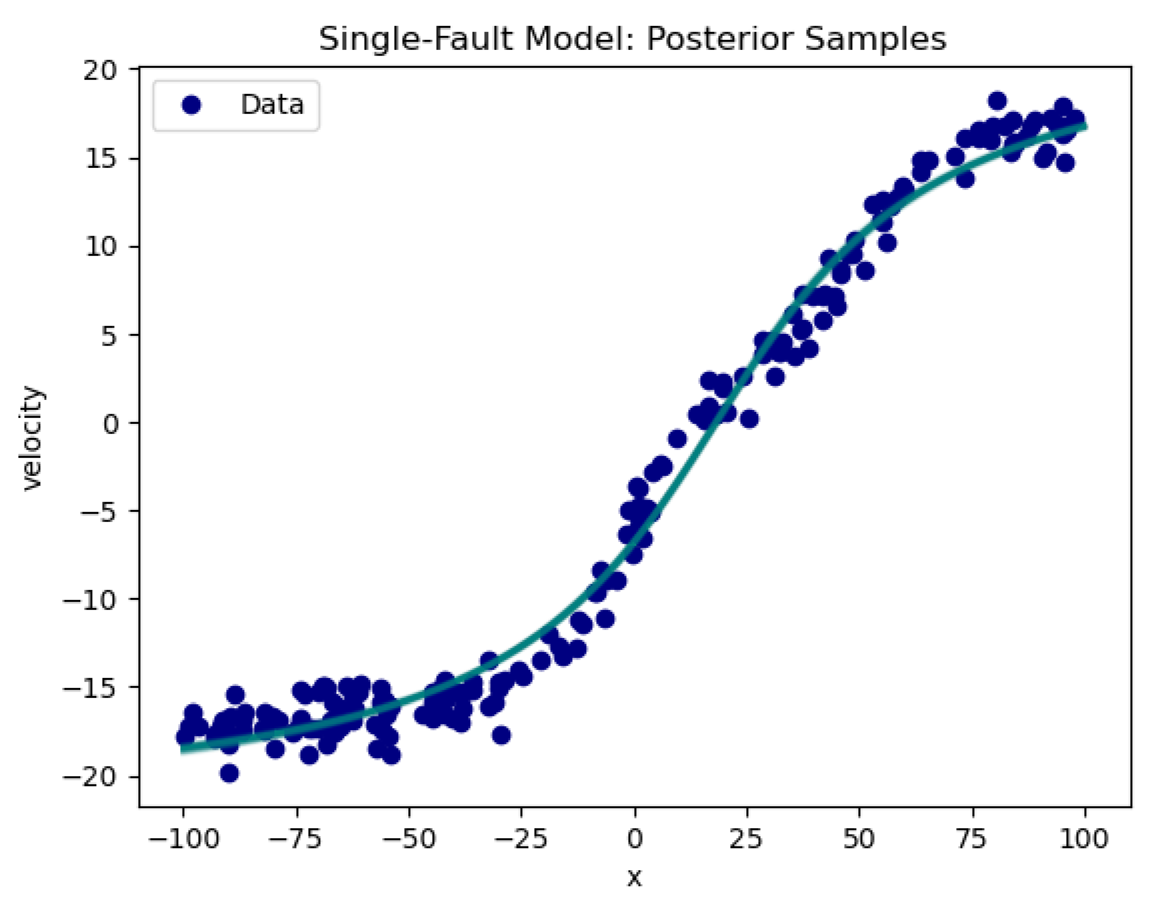
Although not very far from 1, the value of 1.4 for the RMSE is not ideal. Particularly around the origin (see fig. Figure 8), the deviation of data from model become more obvious.
Figure 9.
Two Fault Model Posterior VS Experimental Data. The RMSE is ≈ 1.
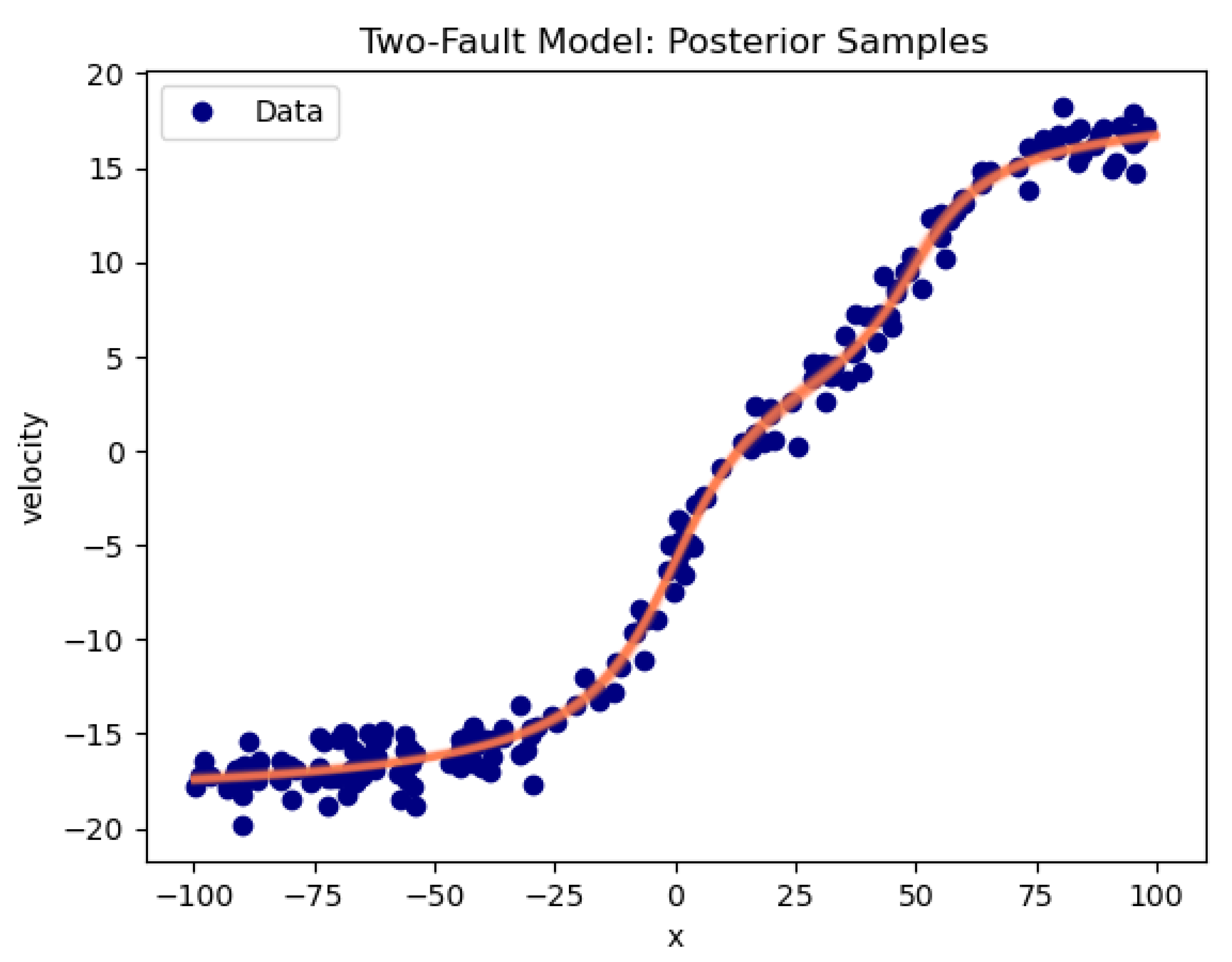
Figure 10.
Two-Fault Model RMSE distribution.
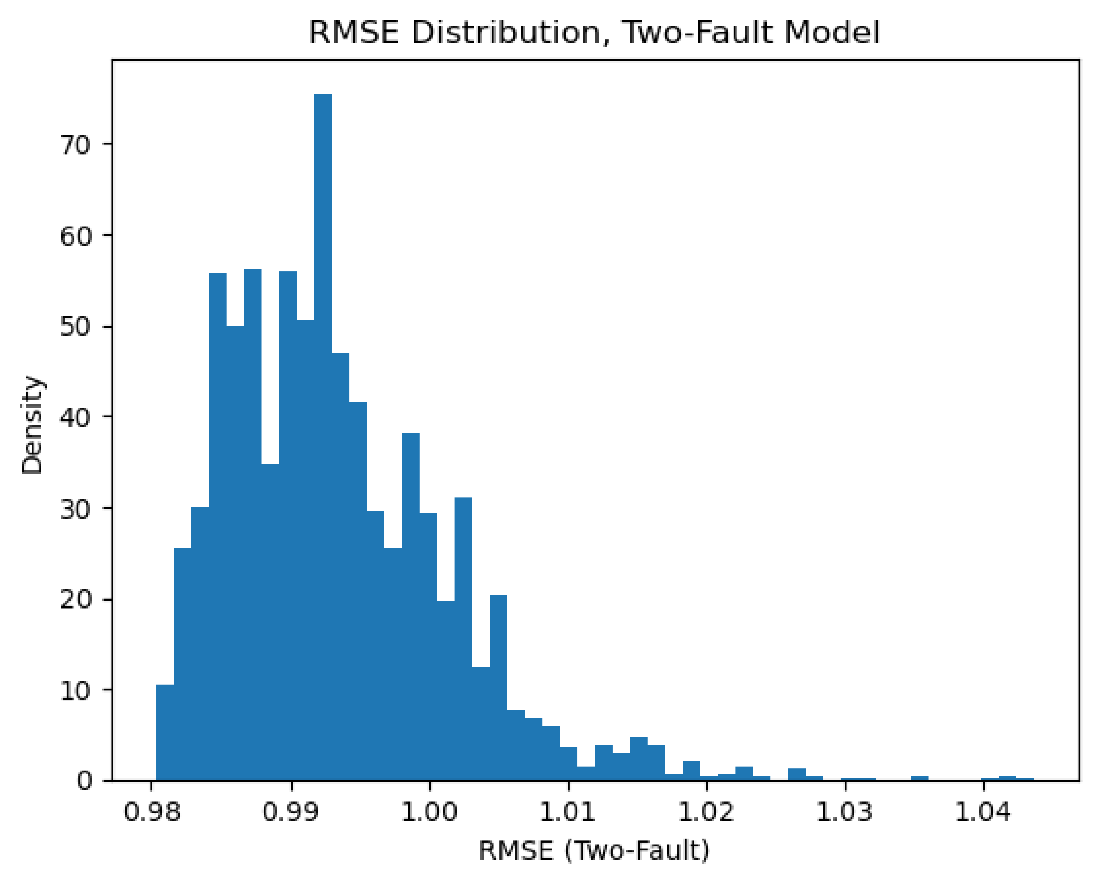
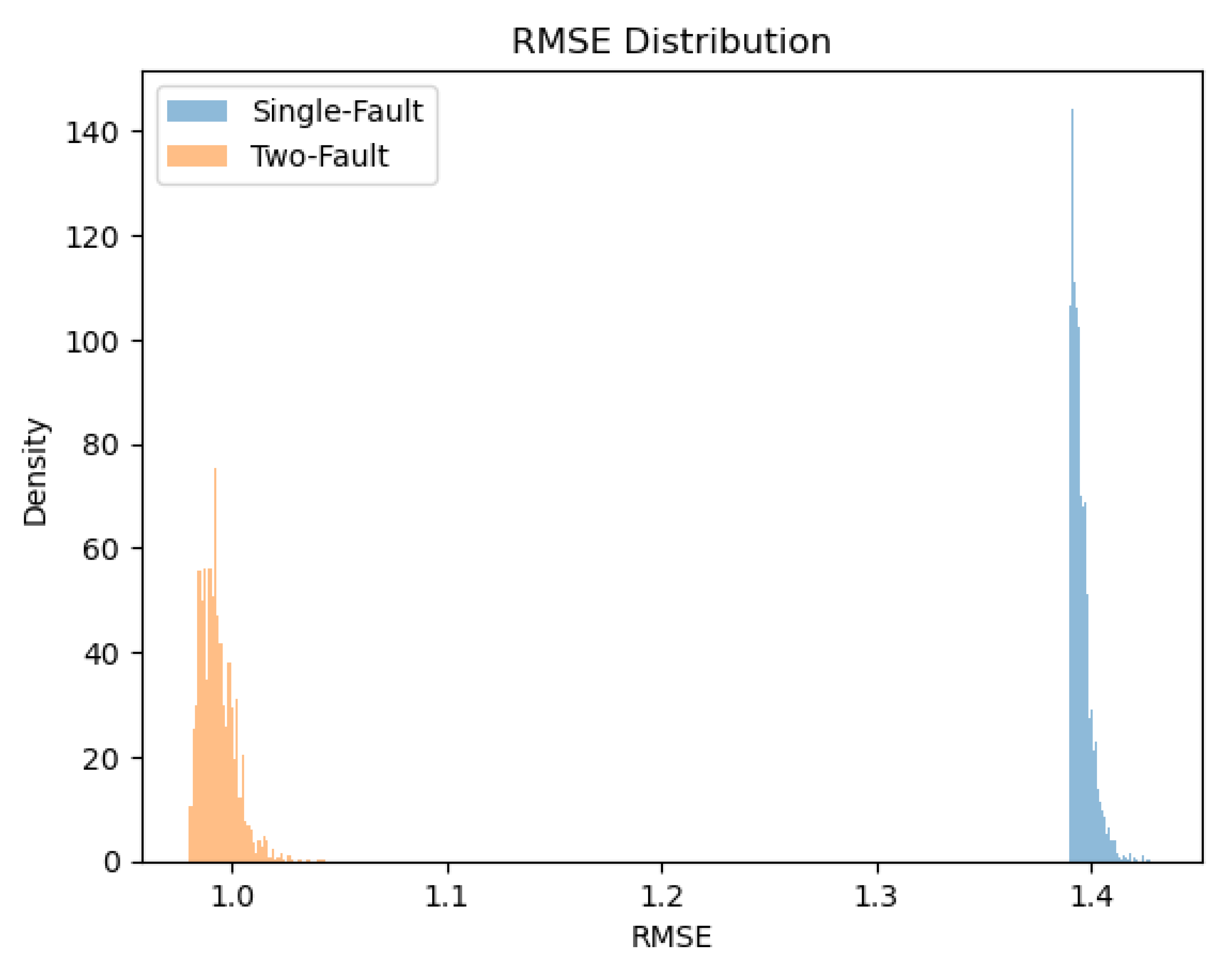
Figure 11.
Two Fault Model RMSE distribution ≈ 1 (Left) VS Single Fault RMSE ≈ 1.4 (Right).
2.12. Fault Analysis: Discussion
Markov Chain Monte Carlo is a powerful method for Data Analysis. In this study, it was used as a tool in Inverse Problem, fitting model parameters to data. This geophysical model elegantly fit to data of 200 points. Using a single-fault model, the parameters were obtained, however with a RMSE of 1.4, which was not ideal. Therefore a Two-fault model was examined, arriving at a RMSE of 1.
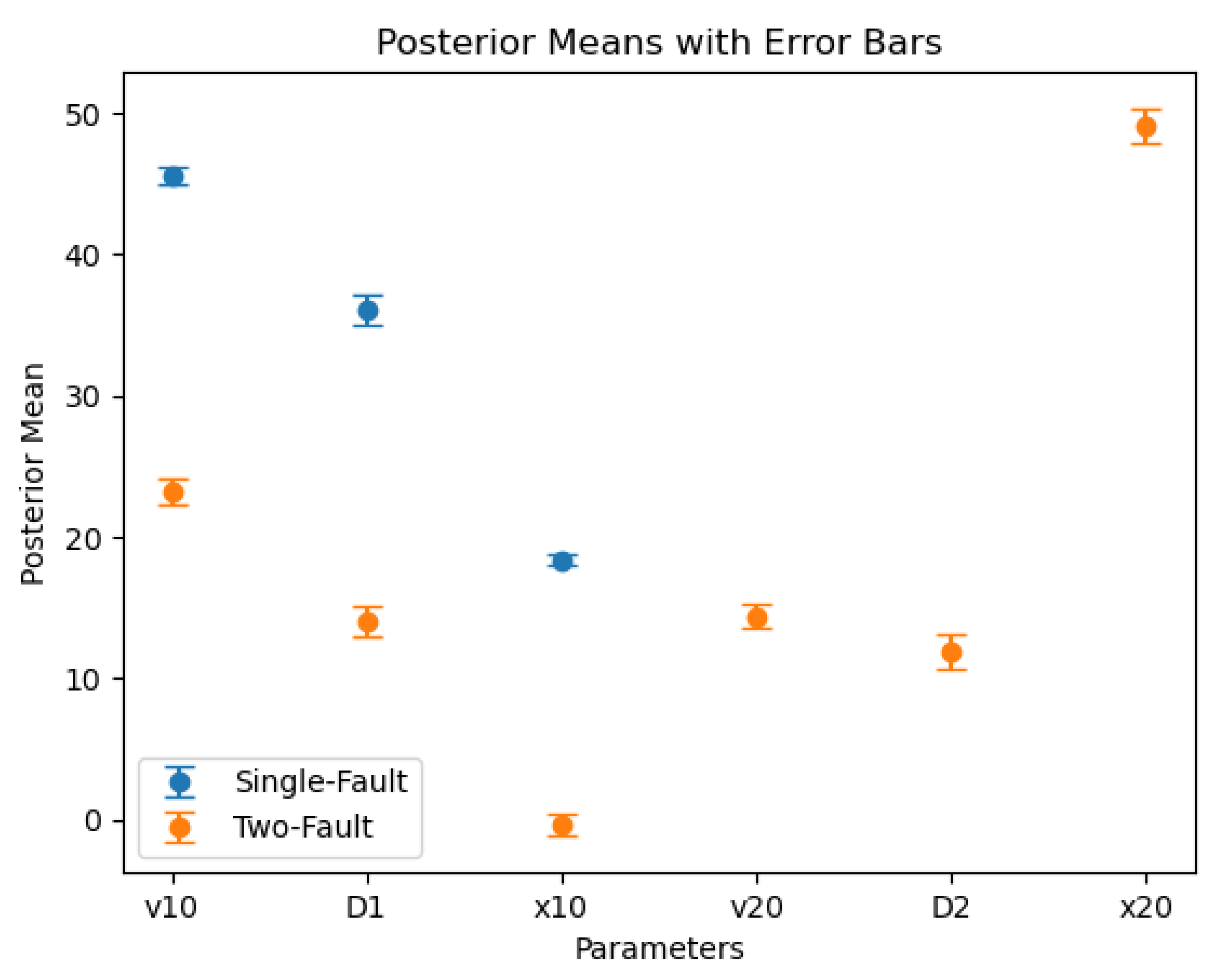
Single Fault Model Parameters are displayed in Table 2.
Which all are within 95 % confidence intervals. These parameters and their error bars are plotted and presented in Figure 12. It can be readily observed that the two models produce two different worldviews for the tectonic movements. The two-fault hypothesis which indicates that the two faults were formed at different times, is also backed by straightforward extrapolation of the record on the ocean floor [34].
Figure 12.
Model Parameter Values and their corresponding uncertainties, within 95 % Confidence Interval
Figure 12.
Model Parameter Values and their corresponding uncertainties, within 95 % Confidence Interval
2.13. Bayesian Hypothesis Testing
Based on new evidence, one can use Bayes’s theorem to update the belief in a hypothesis. It is a powerful method which can be used to improve otherwise non-conclusive tests. The RMSE was already improved to the level of background noise and this can be easily seen comparing Figure 5 and Figure 11, however, Bayesian Hypothesis testing can further improve this. Widely Applicable Information Criterion (WAIC) and Bayesian Information Criterion were both applied. The result, which overwhelmingly favors the Two-fault model is plotted in Figure 13.
3. Anthropogenic Seismicity
Under load, soil does not instantaneously deflect, but changes gradually and at a variable rate. This phenomenon is called consolidation and is mathematically formulated by Biot in 1940 [35]. Hill et. al.[36] argue that stress perturbations in the order of 0.5 MPa are sufficient to trigger seismicity. These perturbations are dominated by pore pressure changes. They furthermore correlated the past 6 major earthquake events on the San Andreas Fault with high-stands of the ancient Lake Cahuilla, which its remnant is known today as the Salton Sea. Using Finite Element Methods (FEM) to arrive at such correlations, their model seems to be applicable to other regions where hydrologic loading is associated with seismicity, anthropogenic or not.
The anthropogenic seismicity risk factor, which I will define as here, (With the physical units of action per unit volume), generally follows an uncertainty relationship:
Where represents the change in pressure and is the time period, with resembling the system’s minimized action per unit volume. This is due to the fact that higher pressures of fluid injections are usually carried out over shorter periods of time and lower pressures are carried out over a larger period of time. In other words, there is a tradeoff. For instance, a larger pressure of wastewater is injected over a short period of time while a smaller pressure of CO2 is associated with CCS operations over longer periods of time. When examined as a complex system, this resembles a path which constraints the system’s evolution in which soil consolidation undergoes dissipation.
A breakdown of these operations and their corresponding share of caused anthropogenic seismicity can be found in Figure 14.
The probability of reservoir-seismicity to be widespread and deeper for a large reservoir is higher than that of a small one [38]. Elevated seismicity in Texas attributed to oil and gas extraction and fluid injections has also been observed [39], which is thought to be caused by pore pressure changes.
CO2 also stimulates plate tectonics due to mechanical pressure excreted by the injected fluids. In the past few years, as part of broader mitigation efforts, CO2 has been injected into the earth. It is postulated that the injected CO2 stays underground for decades. The pressure excreted by this gas can however threaten the integrity of the seals at injection sites. This requires further analysis on the operations as well as more simulations which could shed light on anthropogenic seismicity caused by geological injections.
It is noteworthy that the Los Angeles Oil Field produces about 3.5 barrels of oil per day and also faster than 1 LOS movement on the fault [40].
4. Discussions
Bayesian Inference certainly helps us better understand anthropogenic risks. Modern analysis tools such as the MCMC are therefore certainly useful in shedding light on contemporary problems in Earth Science and particularly inverse problems in geophysics.
Bayesian inference, however, is not a magic black box that could be used for compensating for poorly designed experiments and if information is primarily missing from data, no data analysis tools can reveal information out of thin air. That said, Bayesian inference could be used to better arrange for experimental setups to hunt for information that otherwise could not be captured [41]. This approach can even further improve geophysics experiments which could contribute to the understanding of Earth and planetary processes and anthropogenic risk factors in seismicity.
References
- Turcotte, D.L.; Malamud, B.D. Earthquakes as a complex system. In International Geophysics; Elsevier, 2002; Vol. 81, pp. 209–cp1.
- Sieh, K.; Stuiver, M.; Brillinger, D. A more precise chronology of earthquakes produced by the San Andreas fault in southern California. Journal of Geophysical Research: Solid Earth 1989, 94, 603–623. [Google Scholar] [CrossRef]
- Carpenter, B.; Marone, C.; Saffer, D. Weakness of the San Andreas Fault revealed by samples from the active fault zone. Nature Geoscience 2011, 4, 251–254. [Google Scholar] [CrossRef]
- Collettini, C.; Niemeijer, A.; Viti, C.; Marone, C. Fault zone fabric and fault weakness. Nature 2009, 462, 907–910. [Google Scholar] [CrossRef]
- Moore, D.E.; Rymer, M.J. Talc-bearing serpentinite and the creeping section of the San Andreas Fault. Nature 2007, 448, 795–797. [Google Scholar] [CrossRef] [PubMed]
- Scholz, C.H. Evidence for a strong San Andreas Fault. Geology 2000, 28, 163–166. [Google Scholar] [CrossRef]
- Vilarrasa, V.; Carrera, J.; Olivella, S.; Rutqvist, J.; Laloui, L. Induced seismicity in geologic carbon storage. Solid Earth 2019, 10, 871–892. [Google Scholar] [CrossRef]
- Walker, J.C.; Hays, P.; Kasting, J.F. A negative feedback mechanism for the long-term stabilization of Earth’s surface temperature. Journal of Geophysical Research: Oceans 1981, 86, 9776–9782. [Google Scholar] [CrossRef]
- Penman, D.E.; Caves Rugenstein, J.K.; Ibarra, D.E.; Winnick, M.J. Silicate weathering as a feedback and forcing in Earth’s climate and carbon cycle. Earth-Science Reviews 2020, 209, 103298. [Google Scholar] [CrossRef]
- Archer, D. Fate of fossil fuel CO2 in geologic time. Journal of geophysical research: Oceans 2005, 110. [Google Scholar] [CrossRef]
- Archer, D.; Eby, M.; Brovkin, V.; Ridgwell, A.; Cao, L.; Mikolajewicz, U.; Caldeira, K.; Matsumoto, K.; Munhoven, G.; Montenegro, A.; et al. Atmospheric lifetime of fossil fuel carbon dioxide. Annual review of earth and planetary sciences 2009, 37, 117–134. [Google Scholar] [CrossRef]
- Colbourn, G.; Ridgwell, A.; Lenton, T. The time scale of the silicate weathering negative feedback on atmospheric CO2. Global Biogeochemical Cycles 2015, 29, 583–596. [Google Scholar] [CrossRef]
- Meissner, K.J.; McNeil, B.I.; Eby, M.; Wiebe, E.C. The importance of the terrestrial weathering feedback for multimillennial coral reef habitat recovery. Global Biogeochemical Cycles 2012, 26. [Google Scholar] [CrossRef]
- Keeling, C.D.; Piper, S.C.; Bacastow, R.B.; Wahlen, M.; Whorf, T.P.; Heimann, M.; Meijer, H.A. Exchanges of atmospheric CO2 and 13CO2 with the terrestrial biosphere and oceans from 1978 to 2000. I. Global aspects. SIO Reference Series 01-06, Scripps Institution of Oceanography, San Diego, 2001.
- Church, J.A.; White, N.J.; Konikow, L.F.; Domingues, C.M.; Cogley, J.G.; Rignot, E.; Gregory, J.M.; van den Broeke, M.R.; Monaghan, A.J.; Velicogna, I. Revisiting the Earth’s sea-level and energy budgets from 1961 to 2008. Geophysical Research Letters 2011, 38. [Google Scholar] [CrossRef]
- University of Hawaii Sea Level Center. UHSLC – University of Hawaii Sea Level Center, 2025. Accessed: 2025-04-27.
- Met Office Hadley Centre and Climatic Research Unit. HadCRUT5: Global historical surface temperature anomalies dataset, 2025. Version HadCRUT.5.0.2.0, Accessed: 2025-04-27.
- Batalha, N.E.; Kopparapu, R.K.; Haqq-Misra, J.; Kasting, J.F. Climate cycling on early Mars caused by the carbonate–silicate cycle. Earth and Planetary Science Letters 2016, 455, 7–13. [Google Scholar] [CrossRef]
- Laine, M. Adaptive MCMC methods with applications in environmental and geophysical models; Finnish Meteorological Institute, 2008.
- Malinverno, A. Parsimonious Bayesian Markov chain Monte Carlo inversion in a nonlinear geophysical problem. Geophysical Journal International 2002, 151, 675–688. [Google Scholar] [CrossRef]
- Menke, W. Geophysical data analysis: Discrete inverse theory; Academic Press, 2018.
- Sambridge, M.; Mosegaard, K. Monte Carlo methods in geophysical inverse problems. Reviews of Geophysics 2002, 40, 3–1. [Google Scholar] [CrossRef]
- Trotta, R. Bayes in the sky: Bayesian inference and model selection in cosmology. Contemporary Physics 2008, 49, 71–104. [Google Scholar] [CrossRef]
- Rahemi, R. Variation in electron work function with temperature and its effect on the Young’s modulus of metals. Scripta materialia 2015, 99, 41–44. [Google Scholar] [CrossRef]
- Chang, J.; Nikolaev, P.; Carpena-Núñez, J.; Rao, R.; Decker, K.; Islam, A.E.; Kim, J.; Pitt, M.A.; Myung, J.I.; Maruyama, B. Efficient closed-loop maximization of carbon nanotube growth rate using Bayesian optimization. Scientific reports 2020, 10, 9040. [Google Scholar] [CrossRef]
- Uncertainty quantification of pollutant source retrieval: comparison of Bayesian methods with application to the Chernobyl and Fukushima Daiichi accidental releases of radionuclides 2017. 143, 2886–2901.
- Cluff, L. Photo Credit. Getty Images.
- Menke, W. Geophysical data analysis: Discrete inverse theory; Academic Press, 2018.
- Li, A. Topics In Data Science: Data Analysis In Physics Lectures; Halıcıoğlu Data Science Institute: La Jolla, California, 2025. [Google Scholar]
- Savage, J.C.; Burford, R.O. Geodetic determination of relative plate motion in central California. Journal of Geophysical Research 1973, 78, 832–845. [Google Scholar] [CrossRef]
- Tong, X.; Sandwell, D.; Smith-Konter, B. High-resolution interseismic velocity data along the San Andreas Fault from GPS and InSAR. Journal of Geophysical Research: Solid Earth 2013, 118, 369–389. [Google Scholar] [CrossRef]
- IGPP. Instituge Of Geophysics and Planatary Physics; 2024.
- MORZFELD, M. Geophysical Data Analysis SIOG223- Class Notes; 2024.
- Anderson, D.L. The San Andreas fault. Scientific American 1971, 225, 52–71. [Google Scholar] [CrossRef]
- Biot, M.A. General theory of three-dimensional consolidation. Journal of applied physics 1941, 12, 155–164. [Google Scholar] [CrossRef]
- Hill, R.G.; Weingarten, M.; Rockwell, T.K.; Fialko, Y. Major southern San Andreas earthquakes modulated by lake-filling events. Nature 2023, 618, 761–766. [Google Scholar] [CrossRef] [PubMed]
- Human-Induced Earthquake Database (HiQuake). Induced Earthquakes, 2025. Accessed: 2025-04-27.
- Talwani, P. On the nature of reservoir-induced seismicity. Pure and applied Geophysics 1997, 150, 473–492. [Google Scholar] [CrossRef]
- Deng, F.; Dixon, T.H.; Xie, S. Surface deformation and induced seismicity due to fluid injection and oil and gas extraction in western Texas. Journal of Geophysical Research: Solid Earth 2020, 125, e2019JB018962. [Google Scholar] [CrossRef]
- Argus, D.F.; Heflin, M.B.; Peltzer, G.; Crampé, F.; Webb, F.H. Interseismic strain accumulation and anthropogenic motion in metropolitan Los Angeles. Journal of Geophysical Research: Solid Earth 2005, 110. [Google Scholar] [CrossRef]
- Von Toussaint, U. Bayesian inference in physics. Reviews of Modern Physics 2011, 83, 943–999. [Google Scholar] [CrossRef]
| 1 | Prior Knowledge, or simply the prior: Initial probability distribution assigned to a parameter or hypothesis before observing new data |
Figure 1.
The correlation between variables of concern on Earth, over a few decades (1959-2020) with each data point corresponding to one year, with CO2 as a hue, increasing every year. Higher CO2 concentrations (Filtered annual data from Keeling et. al. [14]) are correlated with higher Sea Levels (As reported by Church 2011 and University Of Hawaii Sea Level Center) [15,16] and higher temperature anomalies (Data from: Met Office H. C. [17]).
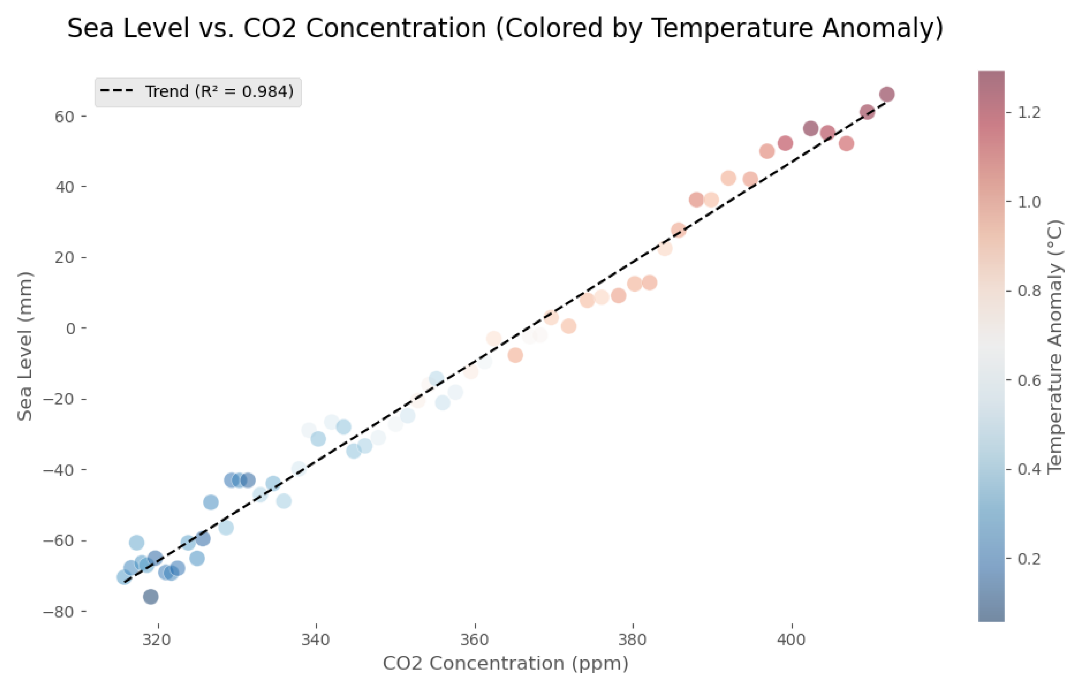
Figure 3.
Location vs Creep rate data is visualized in Cartopy projection using Python. Raw data can be found in ref. [31]. The creep rate peaks between , with a maximum of (mm/year) appearing at .
Figure 3.
Location vs Creep rate data is visualized in Cartopy projection using Python. Raw data can be found in ref. [31]. The creep rate peaks between , with a maximum of (mm/year) appearing at .
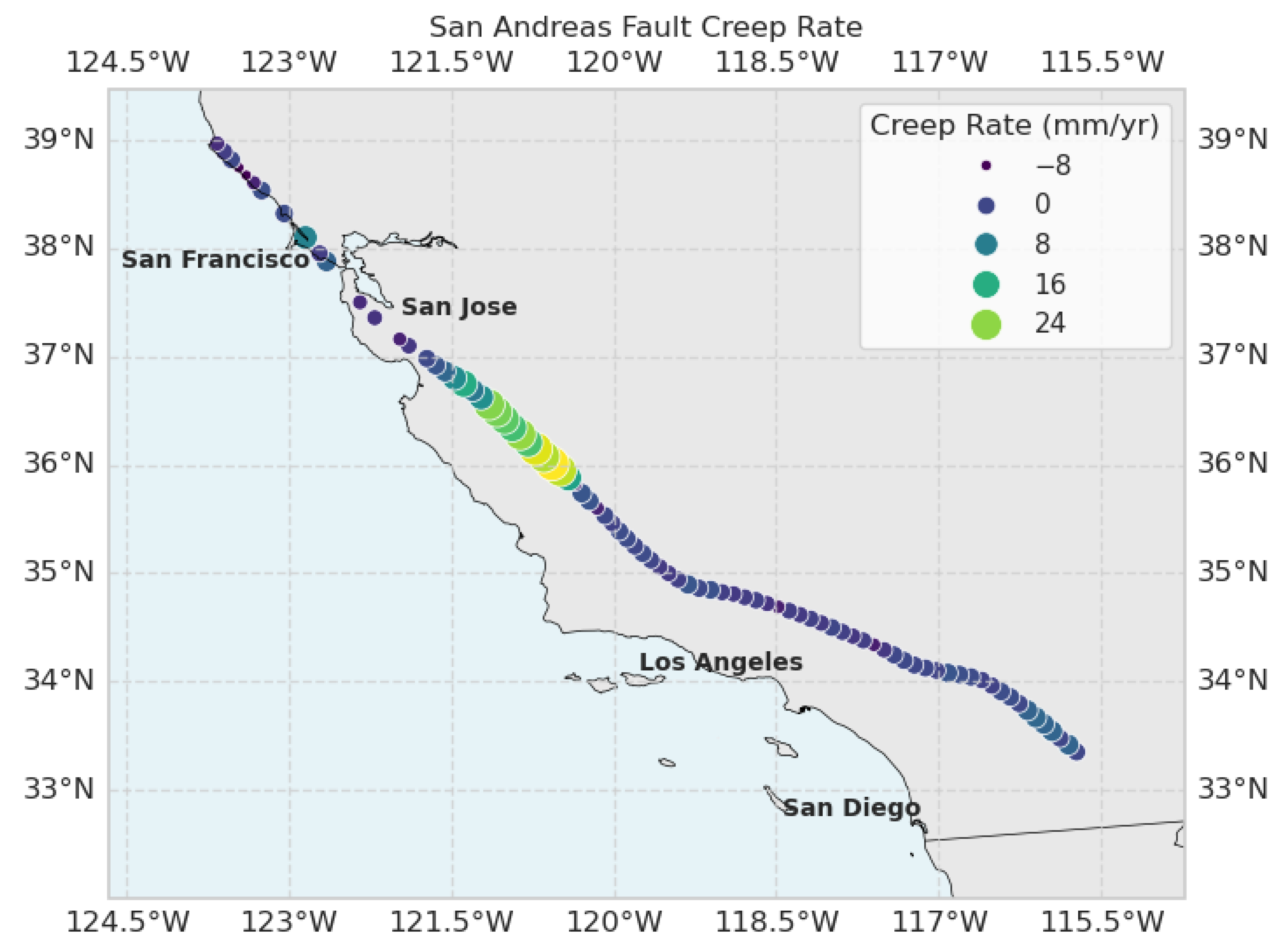
Figure 4.
Creep rate vs Latitude and the corresponding uncertainties. Distributions of the uncertainties are plotted and shown in Figure 5.
Figure 4.
Creep rate vs Latitude and the corresponding uncertainties. Distributions of the uncertainties are plotted and shown in Figure 5.

Figure 6.
Posterior Plot: Visualizing the posterior distribution and correlations. Plotting data and 100 random posterior model curves. First few x values: [-97.922 41.985 95.654 -60.534 -86.19 ] First few v values: [-16.41 7.0886 14.671 -14.797 -16.455 ] Single-fault acceptance rate: . Single-fault posterior means: [45.53 36.05 18.34] Single-fault posterior stds: [0.61 1.13 0.35]
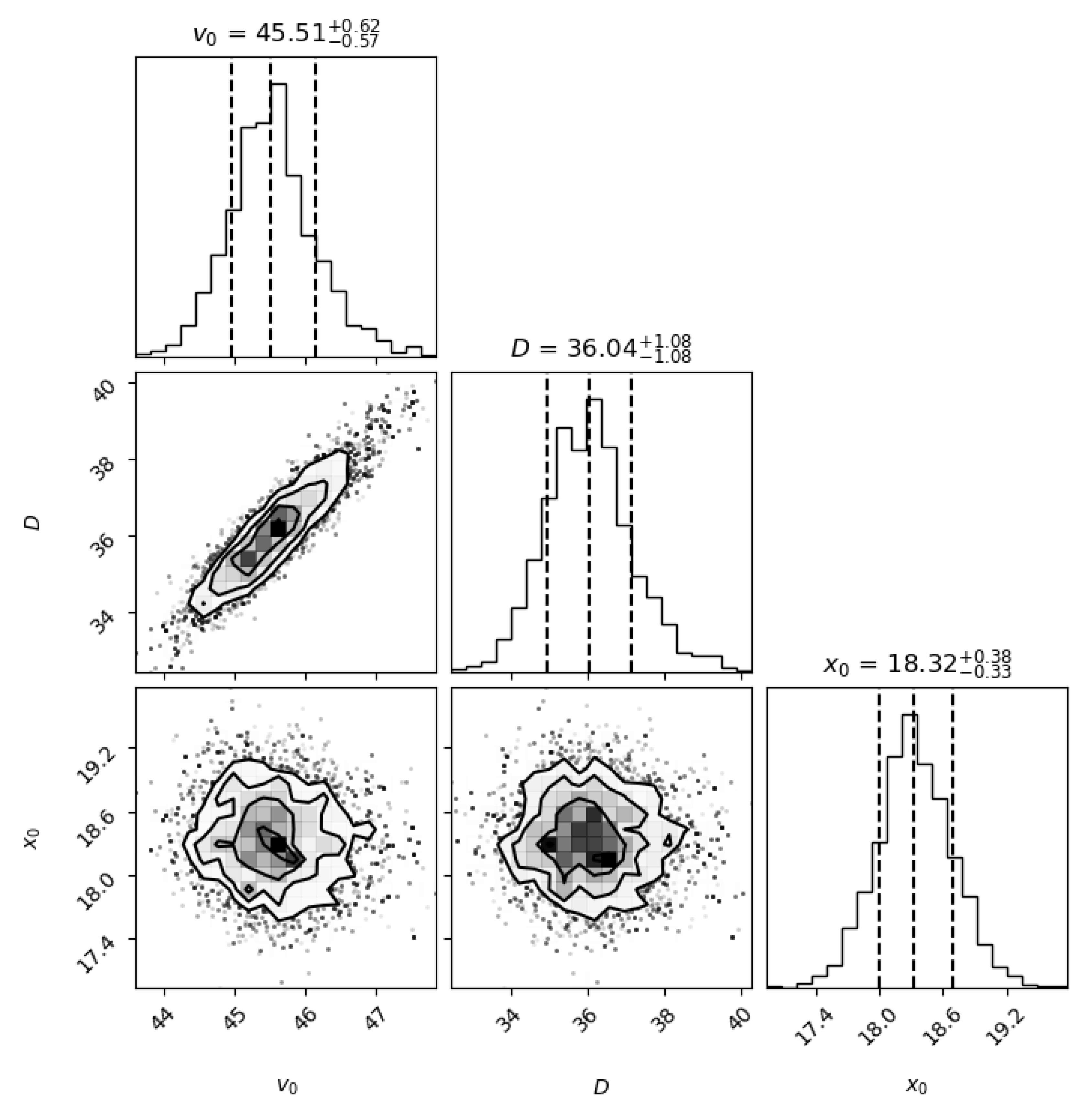
Figure 7.
The negative correlation between the two velocities and are shown here.
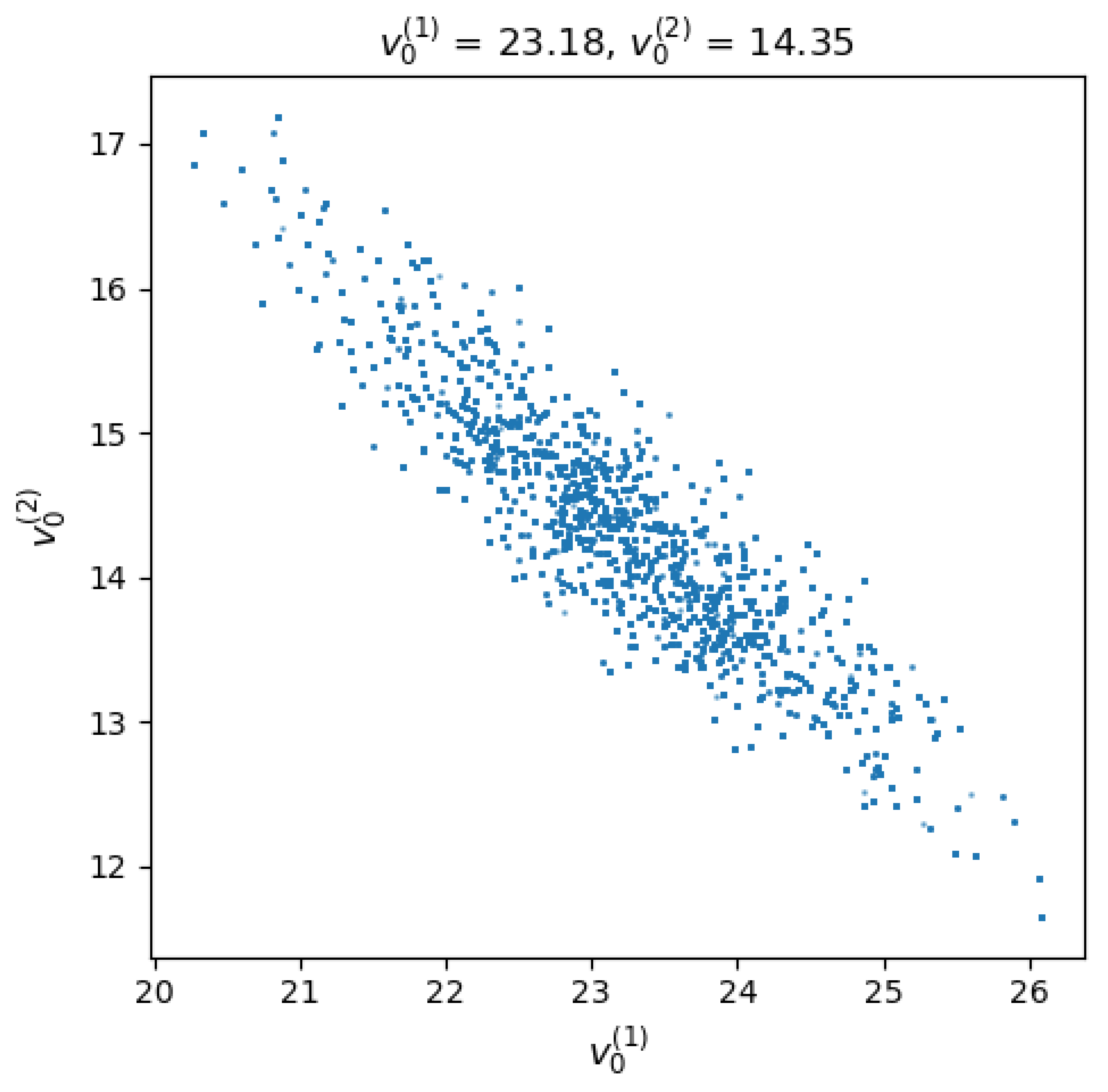
Figure 13.
Comparison of the two models WAIC and BIC, which both favor the Two-Fault model. With lower values in the two methods in favor of the two-faults model.
Figure 13.
Comparison of the two models WAIC and BIC, which both favor the Two-Fault model. With lower values in the two methods in favor of the two-faults model.
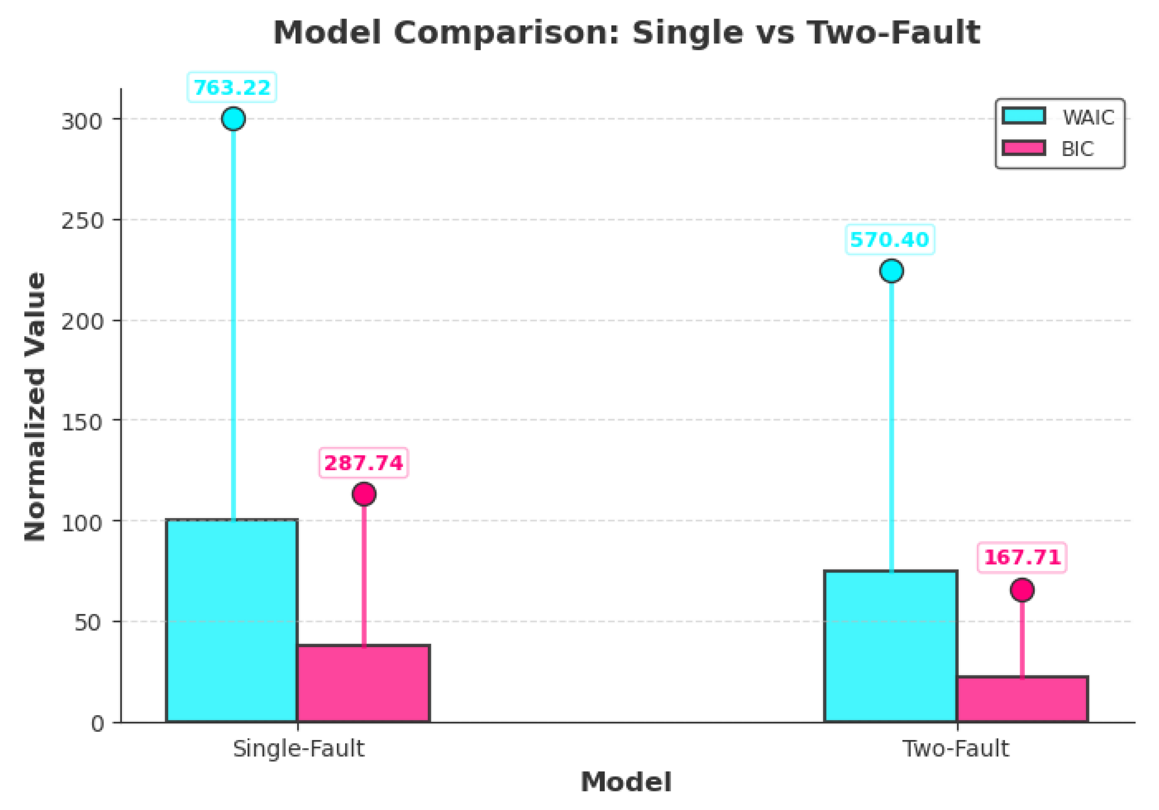
Figure 14.
The share and recorded causes of anthropogenic earthquakes according to the Human Induced Earthquake Database (Hiquake) [37].
Figure 14.
The share and recorded causes of anthropogenic earthquakes according to the Human Induced Earthquake Database (Hiquake) [37].
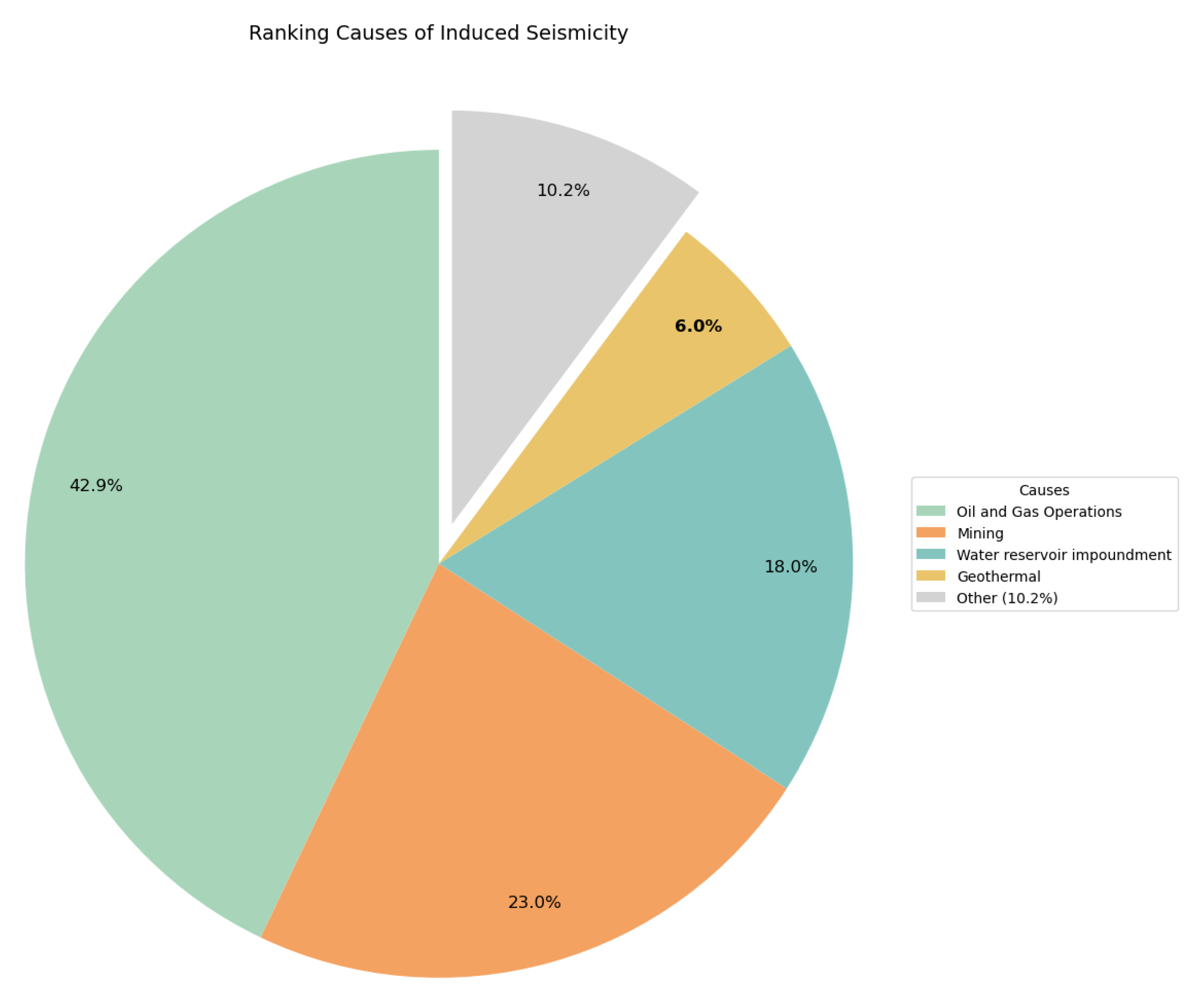

Table 1.
Two Fault Model Parameters.
| 23 ± 1 | |
| 14 ± 1 | |
| - | 0.4 ± 0.8 |
| 49 ± 1 | |
| 14 ± 1 | |
| 12 ± 1 |
Table 2.
Single Fault Model Parameters
| 45.5 ± 0.6 | |
| 18.3 ± 0.4 | |
| D | 36 ± 1.1 |
Disclaimer/Publisher’s Note: The statements, opinions and data contained in all publications are solely those of the individual author(s) and contributor(s) and not of MDPI and/or the editor(s). MDPI and/or the editor(s) disclaim responsibility for any injury to people or property resulting from any ideas, methods, instructions or products referred to in the content. |
© 2025 by the authors. Licensee MDPI, Basel, Switzerland. This article is an open access article distributed under the terms and conditions of the Creative Commons Attribution (CC BY) license (http://creativecommons.org/licenses/by/4.0/).
Copyright: This open access article is published under a Creative Commons CC BY 4.0 license, which permit the free download, distribution, and reuse, provided that the author and preprint are cited in any reuse.


