
Submitted:
29 April 2025
Posted:
29 April 2025
You are already at the latest version
Abstract
The traditional reliance on compressed mathematical notation in machine learning, particularly in calculus-intensive domains such as optimization, presents significant cognitive barriers for both practitioners and students. Core methodologies, such as the Adam optimizer, are widely used in applied settings but are often introduced through dense symbolic expressions that obscure foundational intuitions and hinder practical comprehension. This work proposes a rearticulation of foundational machine learning concepts—including derivatives, gradients, and optimization algorithms, using an intuitive, Pythonic pseudocode paradigm, supported by annotated visual exemplars. By replacing abstract mathematical formalism with code-oriented, formula, inspired explanations, the proposed framework enhances conceptual transparency, operational clarity, and pedagogical accessibility. The overarching goal is to empower developers—particularly those without formal training in advanced mathematics—to internalize, implement, and extend key machine learning constructs with confidence and rigor. In democratizing theoretical understanding, this work seeks to broaden participation in machine learning research and development, fostering a more diverse and interdisciplinary technical community.
Keywords:
Machine Learning education
; Pythonic pseudocode
; accessible machine learning
; optimization algorithms
; gradient descent
; computational thinking
; conceptual understanding
1. Introduction
Mathematics, at its core, constitutes a formal language, an abstract system developed to represent, generalize, and communicate universal patterns and phenomena. Within the field of machine learning, this language is predominantly instantiated through the framework of calculus. Foundational machine learning algorithms are frequently expressed as calculus-based formulations, reflecting a mathematical tradition originating in the 17th century to model continuous and dynamic systems.
In contemporary practice, however, machine learning is primarily instantiated through programming. This evolution has introduced a pronounced disjunction: while many practitioners possess substantial expertise in software engineering and systems design, comparatively few have received formal instruction in the calculus underpinning the algorithms they implement. As a result, the mathematical logic foundational to machine learning often remains opaque, inhibiting developers, even those with advanced technical proficiency, from meaningfully engaging with, modifying, or innovating upon algorithmic structures.
More broadly, this disconnect exacerbates systemic inequities in technical education. A substantial cohort of students, particularly those from under, resourced educational environments, may develop exceptional programming skills yet lack exposure to advanced mathematics. Consequently, access to the deeper strata of machine learning research and development remains uneven, constraining individual opportunity and diminishing the diversity of perspectives essential to innovation in the field.
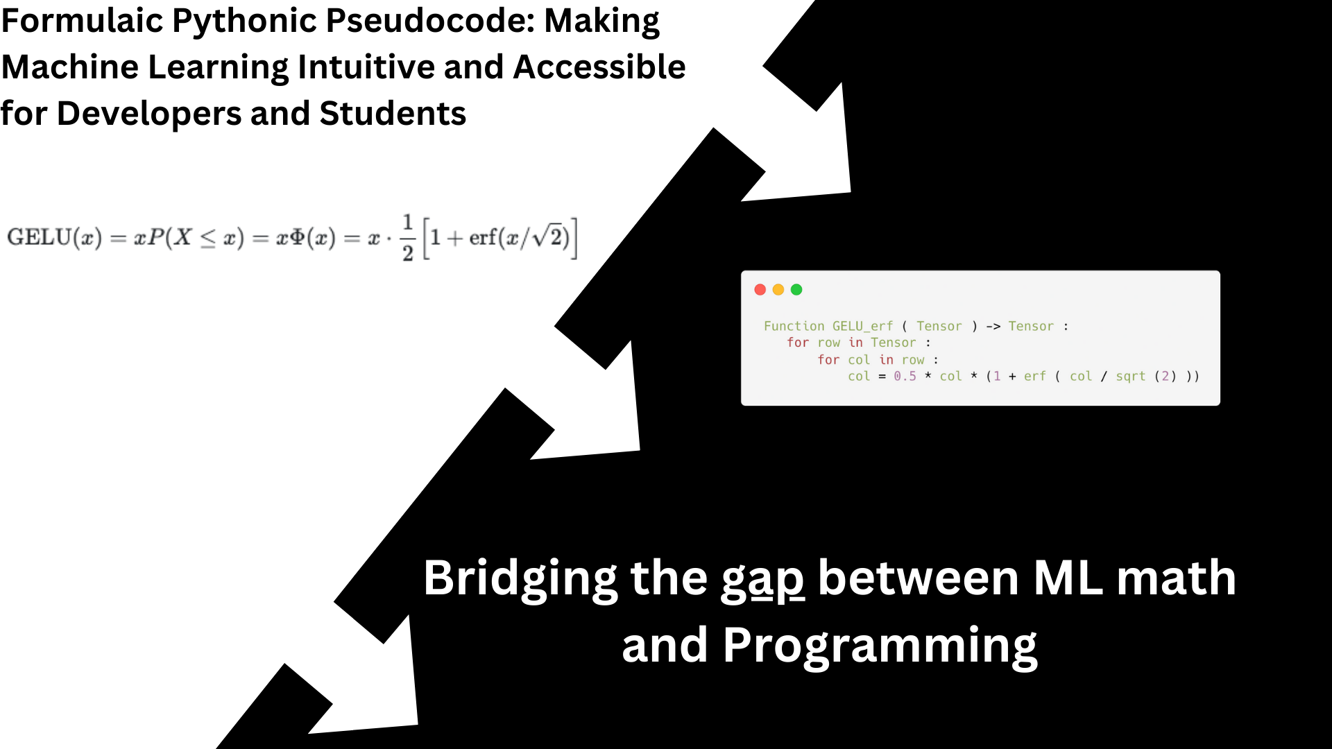
While calculus remains indispensable for theoretical advancements in machine learning, there is a critical need to construct more inclusive and operationally transparent bridges between mathematical theory and computational practice. To this end, this paper introduces Formulaic Pythonic Pseudocode: a structured notation system designed to translate complex calculus, based formulations into accessible, code-oriented representations. This approach preserves mathematical rigor while mitigating the cognitive overhead associated with simultaneously navigating distinct formal systems.
Importantly, the proposed framework is grounded not in ephemeral syntactic conventions, which vary across programming languages, but rather in enduring computational paradigms, such as iterative loops, that mirror fundamental mathematical constructs, including the summation operator (). As such, Formulaic Pythonic Pseudocode constitutes a robust, durable bridge between mathematical abstraction and practical implementation, rendering machine learning theory more transparent, intuitive, and accessible to a broader and more diverse community of developers.
2. Motivation and Background
The development of a machine learning framework in the Rust programming language constituted a significant undertaking in my trajectory as a student researcher. This project necessitated not only the construction of computationally efficient algorithms but also sustained engagement with the advanced mathematical formalism underpinning contemporary machine learning methodologies. The process of translating theoretical formulations into executable systems revealed a series of critical challenges, particularly in navigating the dense and abstract notation prevalent throughout the existing literature.
A focal point of this experience was the implementation of foundational optimization algorithms, such as Adam. The canonical formulations of such algorithms often employ compact symbolic representations that, while mathematically elegant, present formidable barriers to interpretation, even among students with considerable mathematical training. In particular, the standard expression of the Adam optimizer exemplifies this opacity, with many constituent symbols, assumptions, and implied computational steps remaining inaccessible without extensive auxiliary investigation. Through a methodical process of independent research, critical analysis, and iterative refinement, I ultimately derived a fully operational implementation of Adam in Rust, comprising approximately thirty-five lines of source code. The choice of Rust was deliberate, given its capacity to deliver performance comparable to C-based environments while preserving memory safety guarantees and offering a robust ecosystem for build and dependency management.
This experience illuminated a broader structural phenomenon: the persistent disconnect between theoretical macdetailshine learning research and practical software engineering. Although pseudocode is frequently included in academic publications, such representations often approximate condensed calculus more than they resemble executable algorithmic specifications. Essential details, explicit control flow structures, data handling strategies, and operational semantics, are frequently omitted or under-specified, rendering direct translation into code nontrivial and error-prone.
Motivated by these observations, this work seeks to contribute toward narrowing the gap between theoretical exposition and practical implementation. By offering rigorously validated yet accessible algorithmic translations, the project aspires to facilitate deeper engagement with machine learning methodologies among students, software developers, and early-career researchers. It is hoped that these contributions will foster a more integrative understanding of machine learning as both a mathematical discipline and an engineering practice.
The overarching goal is to construct a more inclusive and operationally transparent pathway into the field, beginning with my own contributions.
3. Core Principles
In the development of this work, several core principles were adopted to ensure the accessibility, transparency, and pedagogical rigor of complex Machine Learning concepts. These guiding methodologies are intended to promote a deeper and more intuitive understanding before engaging with formal mathematical expressions.
- Precise Definitions of Foundational Terms: All critical terminology (e.g., weights, gradients) is clearly and systematically defined to establish a consistent conceptual framework.
- Graphical and Diagrammatic Representation: Visual aids, including graphs and diagrams, are utilized extensively to illustrate data flow, transformations, and algorithmic processes, thereby enhancing conceptual clarity.
- Formulaic Pseudocode as a Bridging Mechanism: Pseudocode formulations are employed to systematically bridge abstract mathematical expressions and practical programming logic, facilitating a more intuitive transition from theory to implementation.
- Prioritization of Intuitive Explanations: Initial emphasis is placed on cultivating intuitive understanding before introducing formal mathematical structures, with the goal of reducing cognitive barriers and promoting more effective knowledge transfer.
These principles collectively inform the structure of the paper and reflect a commitment to making Machine Learning education more accessible, particularly for students and practitioners without an extensive background in advanced mathematics.
4. Target Audience
This work is intended for a diverse audience committed to advancing their understanding of Machine Learning, regardless of prior formal exposure to advanced mathematics. The target readership includes:
- High school students embarking on the study of Machine Learning, particularly those seeking accessible and intuitive learning resources.
- Coding bootcamp graduates aiming to deepen their conceptual and practical grasp of Machine Learning beyond standard curricula.
- Software developers and practitioners who possess limited exposure to calculus or higher-level mathematics, yet aspire to implement and innovate within Machine Learning systems.
- Individuals who have encountered challenges with traditional Machine Learning literature, often characterized by excessive formalism and limited pedagogical accessibility.
- Current and future educators interested in re-envisioning Machine Learning instruction models, with an emphasis on enhancing accessibility, transparency, and engagement for emerging generations of developers and researchers.
By explicitly addressing the needs of these groups, this work seeks to bridge existing educational gaps and promote a more inclusive and effective approach to Machine Learning education.
It is not intended for those already fluent in math-heavy Machine Learning theory, rather, it fills the gap for coders who want to go deeper without waiting for university-level math.
5. Vision for the Future of Machine Learning Education
The traditional paradigm for teaching machine learning has historically privileged abstract mathematical formalism, often at the expense of accessibility and inclusivity. While mathematical rigor remains indispensable for the theoretical advancement of the field, an overreliance on abstraction risks alienating a substantial cohort of capable students, practitioners, and developers who might otherwise contribute meaningfully to the discipline.
This work advocates for an alternative educational framework: prioritizing intuition-driven, structured pseudocode alongside annotated visual representations to convey complex machine learning concepts. Such an approach seeks to preserve theoretical depth while significantly enhancing accessibility and conceptual clarity.
I envision a future in which educators, curriculum designers, and self-directed learners adopt intuition-first pedagogical models that lower barriers to entry without sacrificing mathematical integrity. By explicitly bridging the domains of computational logic and mathematical abstraction, it becomes possible to cultivate educational environments wherein intuitive understanding and formal reasoning reinforce one another rather than stand in opposition.
This paper aspires to serve both as a practical resource for learners and as a call to action for educators committed to reimagining the future of machine learning education. A shift toward more inclusive, intuitively structured pedagogy promises not only to democratize access to machine learning expertise but also to accelerate innovation and diversify contributions across the field.
6. Contribution Summary
This paper presents a novel approach to enhancing machine learning accessibility by systematically translating complex, calculus-based concepts into code-oriented pseudocode, designed to mirror real-world programming logic. Central to this contribution is the introduction of Formulaic Pythonic Pseudocode, a notation system specifically engineered to render traditional mathematical formulations accessible to developers without advanced calculus backgrounds by leveraging conventions recognizable across modern programming languages.
Unlike prevailing practices, where pseudocode often mirrors mathematical formalism rather than executable logic, this approach emphasizes programmer-readable structures, enabling comprehension and practical implementation. By facilitating earlier engagement among high school students, coding bootcamp graduates, and early-career developers, the framework aims to expand participation in machine learning model development and foster a more inclusive talent pipeline.
Additionally, this work seeks to establish a new pedagogical standard for machine learning education resources. The proposed framework systematically organizes core machine learning concepts, providing simplified linguistic descriptions, visual representations (such as graphs), detailed breakdowns of constants and hyperparameters, and corresponding Formulaic Pseudocode exemplars. The practical viability of the framework has been demonstrated through its successful application within an independently developed Rust-based machine learning library.
Through these contributions, this paper endeavors to bridge the gap between theoretical exposition and practical engineering, thereby broadening the accessibility, transparency, and operational clarity of machine learning education.
7. Fundations to Machine Learning
Machine Learning is a subfield of artificial intelligence (AI) that focuses on enabling computational systems to automatically identify patterns and structures within large datasets. The core principle of machine learning involves the development of algorithms that allow machines to learn from data, adapt to new information, and make predictions or decisions without being explicitly programmed for every task. In this context, the patterns discovered by the machine are considered a form of intelligence, wherein the system demonstrates the ability to infer relationships, make generalizations, and apply learned knowledge to novel situations.
Machine learning models, often referred to as networks, are typically structured as complex systems of interconnected components. These components, such as neurons and layers, are arranged in various architectures, depending on the specific learning task and algorithm used. The learning process involves a sequence of computational steps, where the system iteratively adjusts internal parameters based on the input data to minimize errors in its predictions or classifications. This process, commonly referred to as training, is essential for the model’s ability to generalize from the training data to unseen data, ensuring its applicability in real-world scenarios.
- Gradient: Refers to a tensor or scalar value that represents the rate of change of a function with respect to its inputs, typically used in optimization algorithms to adjust parameters during training.
- Scalar: A scalar is a tensor with a single parameter or value, often representing a simple quantity such as a real number or a single element within a dataset.
- Vector: A vector is a one-dimensional tensor, typically represented as an array or list of numbers, each corresponding to a distinct quantity within a multi-dimensional space.
- Tensor: A tensor is a multi-dimensional array that generalizes the concept of scalars (zero-dimensional tensors) and vectors (one-dimensional tensors) to higher dimensions, used to represent and store multi-dimensional data structures.
- Target: The target refers to the desired gradient or output value that the model aims to approximate or predict, typically specified in the output layer of a neural network during the training process.
- Output: The output refers to the gradient or value that is produced by the network’s final layer, commonly referred to as the output layer. This value represents the model’s prediction after processing the input through all preceding layers
- Weights, and Bias: Weights and biases are the parameters of each layer within a neural network. Weights represent the strength of the connections between neurons, while biases provide additional offsets to the activation functions. Together, these parameters define the transformation applied to input data as it propagates through the network. Analogous to synapses in the human brain, they control the flow of information within the model.
- Underfitting and Overfitting: Underfitting occurs when a model fails to capture the underlying patterns within the training data, often due to insufficient complexity or inadequate training. Conversely, overfitting arises when a model excessively memorizes the training data, capturing noise and irrelevant details instead of generalizable patterns. This often results in poor performance on unseen data.
- Further sections of this paper provide a more in-depth exploration of these concepts and their implications in the context of neural network training and optimization.
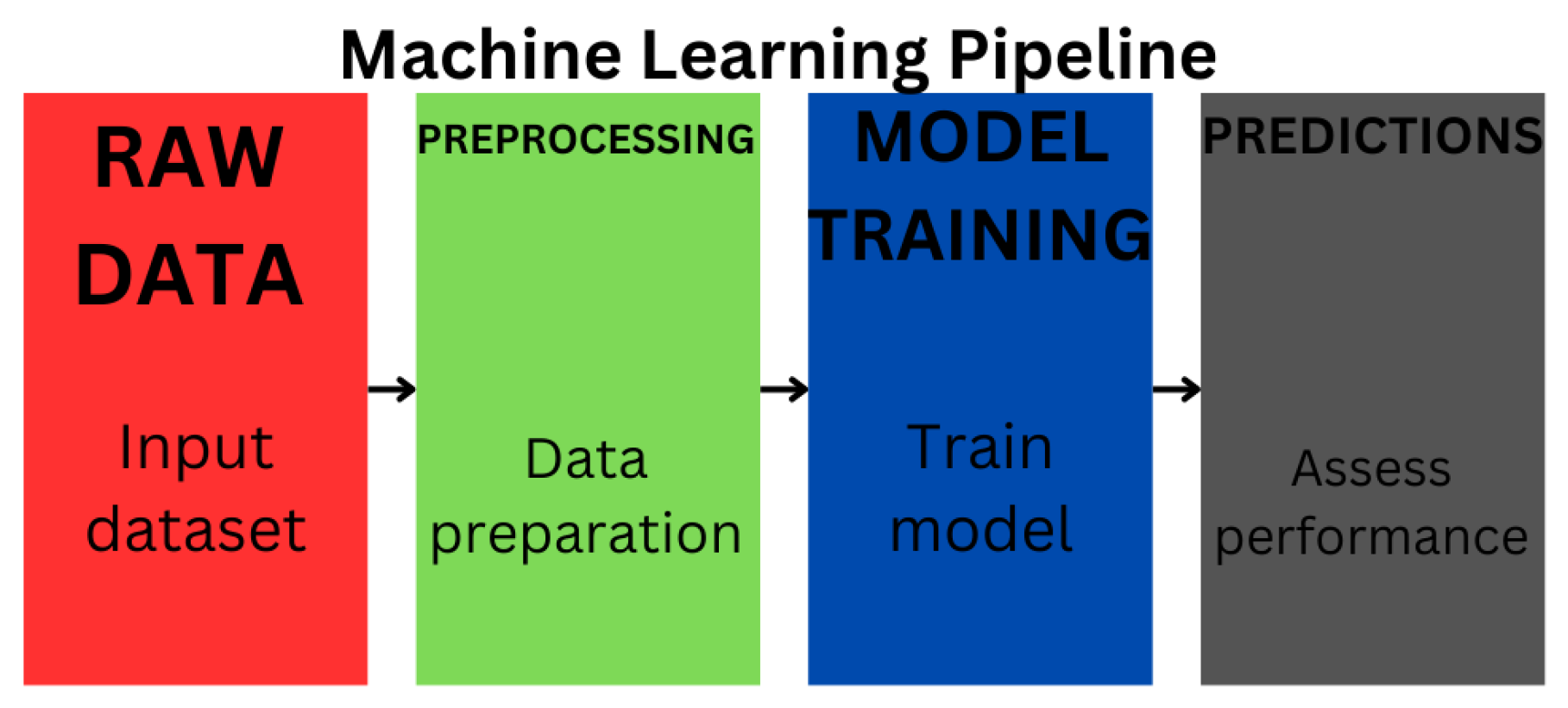
Figure 1.
Neural networks follow the standard Machine Learning pipeline:starting with data collection and preprocessing, followed by model training, validation, and testing, in order to iteratively learn patterns and improve performance over time.
Figure 1.
Neural networks follow the standard Machine Learning pipeline:starting with data collection and preprocessing, followed by model training, validation, and testing, in order to iteratively learn patterns and improve performance over time.
7.1. What can a Tensor store
Tensors can be conceptualized as multi-dimensional arrays that generalize matrices to higher dimensions. Specifically, in the case of two-dimensional tensors, they can be represented as matrices defined by an X and Y axis, effectively forming a grid structure composed of values. In the context of machine learning, it is common to utilize 32-bit floating point representations (float32 or f32) for tensor storage. In certain cases, even lower-precision formats such as half-precision (e.g., float16) may be employed, as the increased precision provided by 64-bit floating point formats (float64 or f64) is often deemed unnecessary for the majority of tasks. The adoption of lower-precision formats offers a significant advantage in reducing memory consumption and computational overhead, while maintaining the performance of the model in most practical applications. This trade-off between precision and efficiency is a critical consideration in the design and implementation of machine learning models, especially when scaling to large datasets or complex architectures.
7.2. Layer in a Machine Learning Context
A neural network is inherently composed of multiple layers, each playing a critical role in the transformation and processing of input data. Within each layer, there exist two fundamental components: the weight tensor and the bias tensor. The weight tensor governs the scaling of input signals, determining the strength and direction of the connections between neurons. Conversely, the bias tensor facilitates the network’s ability to model complex, non-linear relationships, enabling the network to capture patterns that cannot be represented through weighted inputs alone. Together, these components allow the network to approximate highly intricate functions, making it capable of learning from data in a manner that transcends simple linear transformations.
7.3. Neural Network
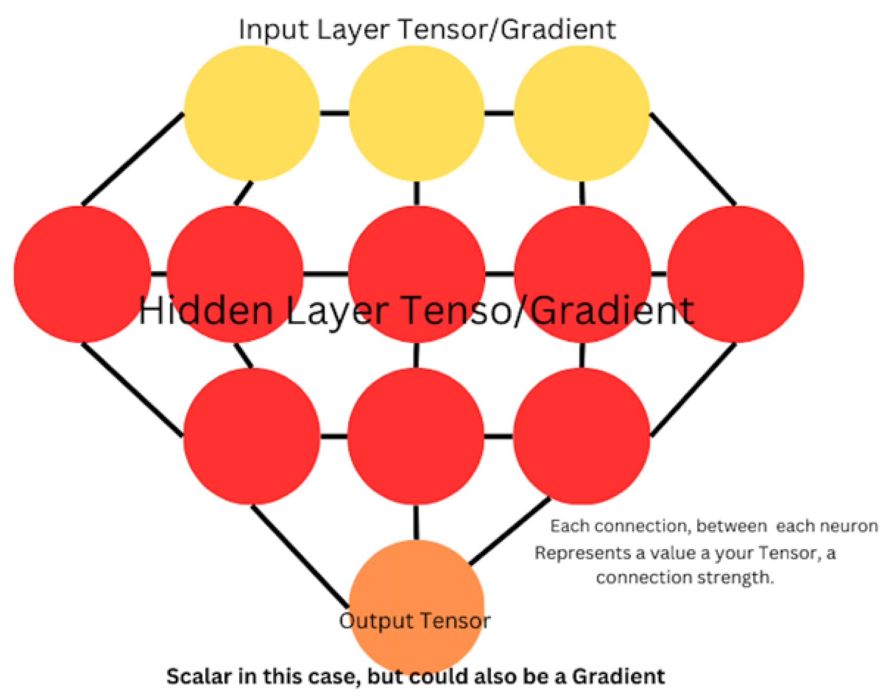
Figure 2.
Basic structure of a fully connected neural network, comprising the Input, Hidden, and Output layers. Each layer is represented as a set of neurons, with each neuron in one layer being connected to every neuron in the subsequent layer.
Figure 2.
Basic structure of a fully connected neural network, comprising the Input, Hidden, and Output layers. Each layer is represented as a set of neurons, with each neuron in one layer being connected to every neuron in the subsequent layer.
7.3.1. Understanding the Neural Network
Notice how each weight/neuron within the network is connected to nearby neurons in the adjacent top and bottom layers.
- Input: Accepts raw data, which can be normalized to prevent gradient issues.
- Hidden: Applies matrix multiplication to propagate signal strengths throughout the network.
- Output: Produces the final prediction, which can be compared to the target to compute the network error.
Training Steps Overview: The training of neural networks involves a systematic procedure that ensures the model learns effectively from the data. The steps outlined below describe the critical stages in this process:
- Data Collection and Preprocessing: A fundamental prerequisite for training a neural network is the acquisition of a clean, well-prepared dataset. This involves identifying and removing significant outliers and ensuring that the input features are correctly paired with their corresponding target values. The integrity of the data must be preserved to avoid introducing noise that could impair model performance.
- Model Architecture Definition: The next step is to design the architecture of the neural network. This includes the selection of layer types (such as Dense, Convolutional, or Recurrent layers), determining the number of layers, and specifying the number of units within each layer. Additionally, appropriate activation functions must be chosen for each layer to enable the model to learn complex relationships within the data.
- Loss Function Selection: The choice of a loss function is crucial for quantifying the error between the predicted outputs and the actual target values. Common loss functions include Mean Squared Error (MSE) for regression tasks and Mean Absolute Error (MAE), among others. The loss function serves as the objective that the network aims to minimize during training.
- Optimizer Selection: To optimize the learning process, an optimizer must be chosen to adjust the network’s weights. Algorithms such as Adam are commonly used due to their adaptive learning rates and effective convergence properties. The optimizer adjusts the learning rate dynamically to ensure efficient convergence based on the gradients computed during backpropagation.
- Foward Pass: During the forward pass, input data is propagated through the network. Each layer computes an activation function, transforming the input data at each stage. The final layer produces the predicted output, which is compared to the true labels or target values.
- Loss Computation: Once the forward pass is complete, the predicted output is evaluated against the true target values using the selected loss function. This step quantifies the difference between the predicted and actual values, providing a measure of the model’s performance.
- Backward Pass (Backpropagation): The backward pass involves calculating the gradients of the loss function with respect to the network’s weights. This is achieved by applying the Chain Rule of calculus to propagate the error backward through the network, layer by layer, to compute the necessary gradients.
- Weight Update: The optimizer is then used to update the network’s weights and biases based on the gradients computed during the backward pass. This iterative process continues until the model converges to a solution that minimizes the loss function.
This work provides dedicated sections that systematically examine each of these processes in greater detail. The Forward Pass, Loss Computation, and Backward Pass are presented as essential phases within the broader Backpropagation framework, which constitutes the core mechanism enabling neural networks to iteratively refine their parameters and thereby learn from data.
8. Tensors
In the context of Machine Learning, tensors serve as a foundational mathematical structure for representing and manipulating data across multiple dimensions. Although tensors are frequently utilized to encode gradients the derivatives of functions with respect to their parameters their utility extends far beyond this application. More generally, tensors provide a unified and systematic framework for modeling multi-dimensional data arrays, irrespective of dimensional complexity.
This intrinsic versatility enables tensors to facilitate the efficient storage, transformation, and computation of complex datasets within modern computational models. As such, tensors are indispensable not only for the theoretical formulation of Machine Learning algorithms but also for their practical implementation across a wide range of applications. Their role as a bridge between abstract mathematical formalism and applied algorithmic processes underscores their centrality in contemporary Machine Learning research and practice.
- Constituent Components of Tensors: Tensors are composed of several interrelated structural elements that define their behavior and application within computational frameworks.
- Dimension: In most Machine Learning contexts, tensors are utilized in their two-dimensional (2D) form. This paper primarily focuses on two-dimensional tensors; however, the conceptual principles discussed are extensible to tensors of higher dimensions.
- Shape: The shape of a two-dimensional tensor (matrix) is characterized by two parameters: the number of rows (X-axis) and the number of columns (Y-axis). This structure determines the organizational layout of the data within the tensor.
- Parameters: The total number of parameters within a tensor is defined as the product of its dimensions, calculated as rows × columns. This quantity corresponds to the total number of individual elements or connections represented.
- Weights: In neural network architectures, the primary tensor associated with each layer is referred to as the weights tensor. These tensors encode the learnable parameters that are updated during the training process.
- Bias: Complementing the weights tensor, the bias tensor is introduced at each layer to enable additional model complexity and flexibility, allowing the network to better capture patterns in the data.
- Scalar vs. Gradient: A tensor consisting of a single element with a shape of is classified as a scalar. In contrast, gradients tensors representing derivatives with respect to model parameters generally possess higher-dimensional shapes and necessitate iteration mechanisms (e.g., loops) for computation across their elements.
- Logits: Logits refer to the raw, unnormalized output values produced by a neural network layer, typically represented within tensors prior to the application of activation functions such as softmax or sigmoid.
- Element: An element denotes a single numerical value contained within a tensor, identified by its unique position according to the tensor’s dimensional structure.
Certain tensor operations necessitate the use of broadcasting, a process by which tensor shapes are automatically expanded to ensure compatibility for element-wise computations. Broadcasting is particularly critical for operations such as matrix multiplication, where the participating tensors must conform to specific dimensional requirements to permit valid arithmetic operations.
The type and complexity of tensor operations applied—ranging from scalar interactions to vector and matrix (two-dimensional tensor) manipulations are determined by both the architectural design of the network and the underlying computational objectives. Careful management of tensor shapes and operations is therefore essential to maintaining the mathematical integrity and efficiency of Machine Learning models.
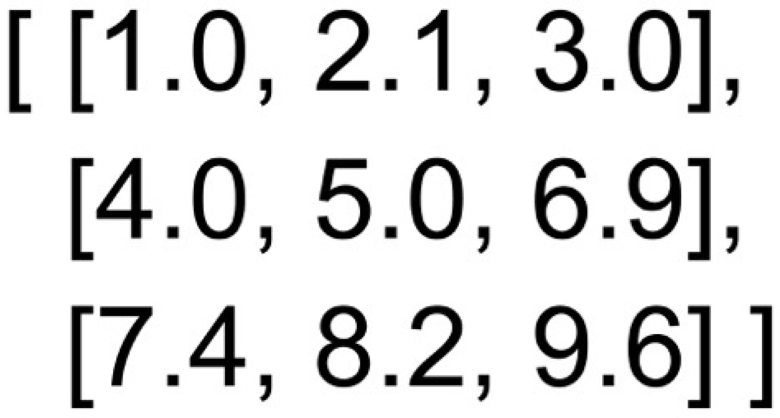
Figure 3.
Example: Tensor/Matrix/Gradient, with shape: (3,3), Parameters: 9, Sum: 47.2.
8.1. Key Gradient Pathologies
During the Machine Learning training pipeline, gradients are subjected to repeated multiplication across multiple layers and operations. As a consequence, their magnitudes can either grow uncontrollably or diminish to near-zero values, leading to severe numerical instabilities. Two primary types of gradient pathologies are typically observed:
- Exploding Gradients: This phenomenon occurs when the magnitudes of tensor elements increase exponentially during backpropagation, potentially exceeding the representational limits of the specified data type and causing numerical overflow or instability.
- Vanishing Gradients: Conversely, vanishing gradients arise when the magnitudes of tensor elements diminish exponentially, approaching zero and resulting in numerical underflow. This leads to stagnation in learning, as weight updates become negligibly small.
Mitigating these issues is crucial for ensuring stable and effective neural network training, and various architectural and optimization strategies have been developed to address them.
8.2. Tensor Rank Versus Tensor Shape
Although often colloquially interchanged, the concepts of rank and shape possess distinct meanings within the context of Machine Learning and tensor operations:
- Rank (Order): The rank of a tensor refers to the number of dimensions it possesses. For example, a scalar has rank 0, a vector has rank 1, and a matrix has rank 2.
- Shape: The shape of a tensor specifies the explicit size of each dimension. For instance, a tensor with a shape of has three rows and five columns in its two-dimensional representation.
A clear understanding of the distinction between rank and shape is essential for designing and debugging Machine Learning models, as errors in dimensional reasoning frequently underlie operational failures.
8.3. Axis Operations
In tensor algebra, operations along Axis 0 are performed row-wise, whereas operations along Axis 1 are performed column-wise. For tensors of higher dimensionality (i.e., rank greater than two), subsequent axes correspond to progressively deeper structural layers, following the same organizational pattern. A clear understanding of axis conventions is critical for correctly implementing tensor manipulations and avoiding shape-related computational errors.
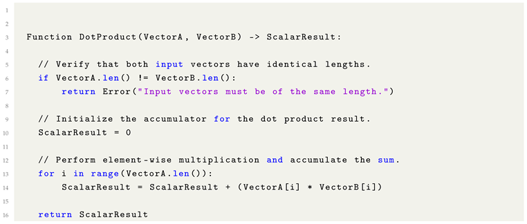
8.4. Dot Product
The dot product is a fundamental operation in linear algebra, particularly relevant to Machine Learning applications involving vector and matrix computations. It is defined as the sum of the element-wise products of two vectors occupying parallel positions within their respective structures.
| Listing 1. Formulaic Pythonic Pseudocode for Dot Product Computation. |
 |
Use Cases of the Dot Product
- Aggregating features within neural network architectures, particularly in fully connected (dense) layers.
- Computing the angle between two vectors, which provides insights into their directional alignment.
- Serving as the basis for cosine similarity, a common metric for comparing vector representations in tasks such as information retrieval and recommendation systems.
Interpreting the Results
- A large positive result indicates strong agreement between the vectors (i.e., vectors oriented in similar directions).
- A negative result reflects opposing directions, suggesting that the vectors are substantially misaligned.
- A result close to zero indicates orthogonality (perpendicularity) between the vectors, implying the absence of linear correlation.
A thorough understanding of the dot product is foundational for operations such as fully connected layers, similarity-based retrieval methods, and various forms of vector space modeling within Machine Learning.
Figure 4.
Tensor Addition.
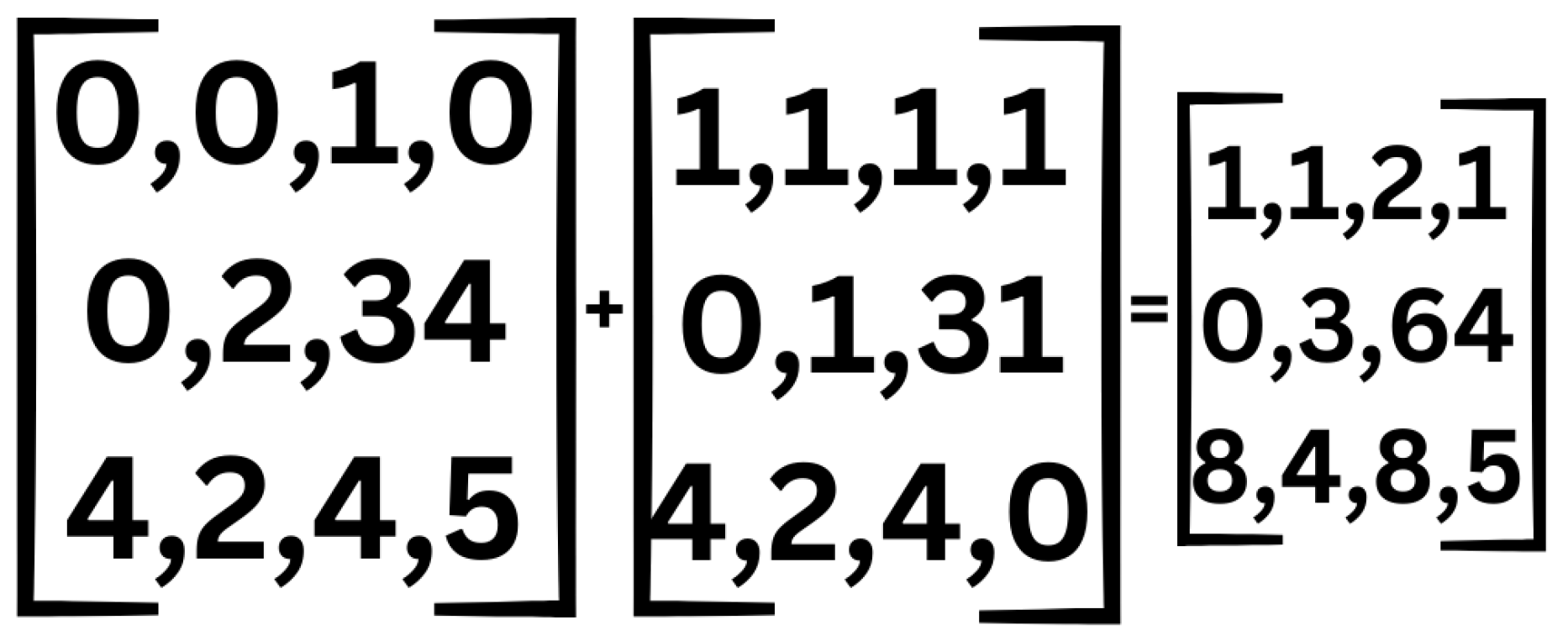
8.5. Tensor Addition
Tensor addition is a fundamental operation wherein two tensors are combined through element-wise summation. Given two tensors of compatible shapes, the addition operation is performed by adding corresponding elements from each tensor.
Unlike tensor multiplication and division, which impose stricter constraints on dimensional compatibility, tensor addition can be applied between tensors of different shapes through broadcasting, provided that the shapes align according to broadcasting rules. This flexibility makes tensor addition particularly useful for constructing and manipulating complex computational structures within Machine Learning models.
| Listing 2. Formulaic Pythonic Pseudocode for Tensor Addition. |
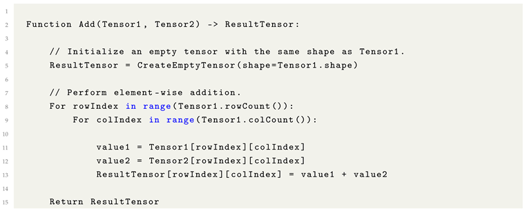 |
Tensor addition is widely utilized in Machine Learning workflows for a variety of purposes. It can be employed to merge gradients or feature representations during training, as well as to incorporate bias vectors into the outputs of neural network layers.
Additionally, tensor addition plays a critical role in broadcasting operations, enabling tensors of differing shapes to be expanded to a common shape. This alignment is essential for performing matrix-wise operations that require shape compatibility between operands.
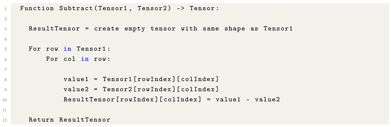
8.6. Tensor Subtraction
Tensor subtraction constitutes an element-wise operation wherein corresponding elements from two tensors are subtracted. Structurally, it mirrors the process of tensor addition, differing only in the arithmetic operation applied.
Given two tensors of compatible shapes, subtraction is performed by subtracting each element of the second tensor from the corresponding element of the first tensor. This operation maintains dimensional consistency and is fundamental in a variety of Machine Learning contexts, such as calculating residuals, adjusting feature maps, or implementing optimization updates.
| Listing 3. Formulaic Pythonic Code for Tensor Subtraction. |
 |
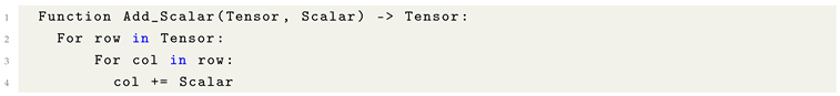
8.7. Scalar Addition
Scalar addition in the context of tensors typically involves an element-wise operation, where a scalar value is added individually to each element of the tensor. This approach results in a uniform transformation across all entries, preserving the relative structure of the original tensor while uniformly shifting its values.
Alternatively, scalar addition can be implemented via tensor broadcasting, wherein the scalar is implicitly expanded to match the shape of the tensor. While broadcasting enables computational efficiency, the scalar’s impact may be perceived as minimal, particularly at specific coordinates (e.g., ), where its relative contribution may be diminished by the broader dimensional context.
| Listing 4. Formulaic Pythonic Code for Scalar Addition. |
 |
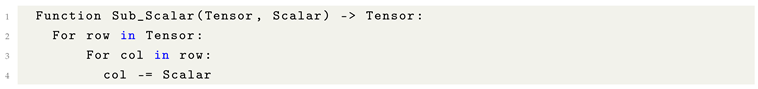
8.8. Scalar Subtraction
One common way to perform Scalar Subtraction is through element-wise operations across an entire tensor, with the result updating the element. In this approach, the scalar value is substracted individually to each element of the tensor. This ensures a uniform transformation throughout the tensor. Alternatively, a scalar can be subtracted using tensor broadcasting during tensor subtraction, but this often results in the scalar having minimal impact, especially at specific coordinates like (x1, y2), where its effect may be diluted by the dimensional context.
| Listing 5. Formulaic Pythonic Code for Scalar Subtraction. |
 |
8.9. Scalar Multiplication
Scalar multiplication constitutes an element-wise operation in which a scalar value is multiplied with each individual element of a tensor. Structurally, it mirrors tensor addition and subtraction in that the operation is applied uniformly across all tensor indices; however, the arithmetic operation performed is multiplication.
This technique enables uniform scaling of tensor values and is fundamental in a variety of Machine Learning applications, including feature normalization, gradient scaling, and adjusting activation outputs.
| Listing 6. Formulaic Pythonic Pseudocode for Scalar Multiplication. |
 |
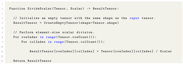
8.10. Scalar Division
Scalar division constitutes an element-wise operation analogous to scalar multiplication, differing only in the arithmetic operation applied. Instead of multiplying each element of a tensor by a scalar, each element is divided by the scalar value.
This operation is commonly employed for normalization tasks, scaling tensor values to a desired range, and adjusting model parameters during optimization procedures.
| Listing 7. Formulaic Pythonic Pseudocode for Scalar Division. |
 |
8.11. Use Cases of Tensor-Scalar Operations
Tensor-scalar operations are critical components in Machine Learning workflows, serving to reduce complex multi-dimensional structures into singular, interpretable scalar values. These operations underpin several fundamental aspects of modern computational models, including:
- Loss Functions: Quantifying prediction errors by aggregating differences between predicted and actual outputs into a single optimization target.
- Evaluation Metrics: Assessing model performance through scalar scores such as accuracy, precision, recall, or F1 score.
- Regularization Terms: Penalizing model complexity by incorporating scalar-valued norms (regularization) into the loss function to encourage simpler models.
- Gradient Aggregation: Summarizing parameter updates across batches or layers to stabilize and guide the optimization process.
- State Monitoring: Tracking statistical properties of tensors, such as mean, variance, or norm, to facilitate model diagnostics and performance tuning.
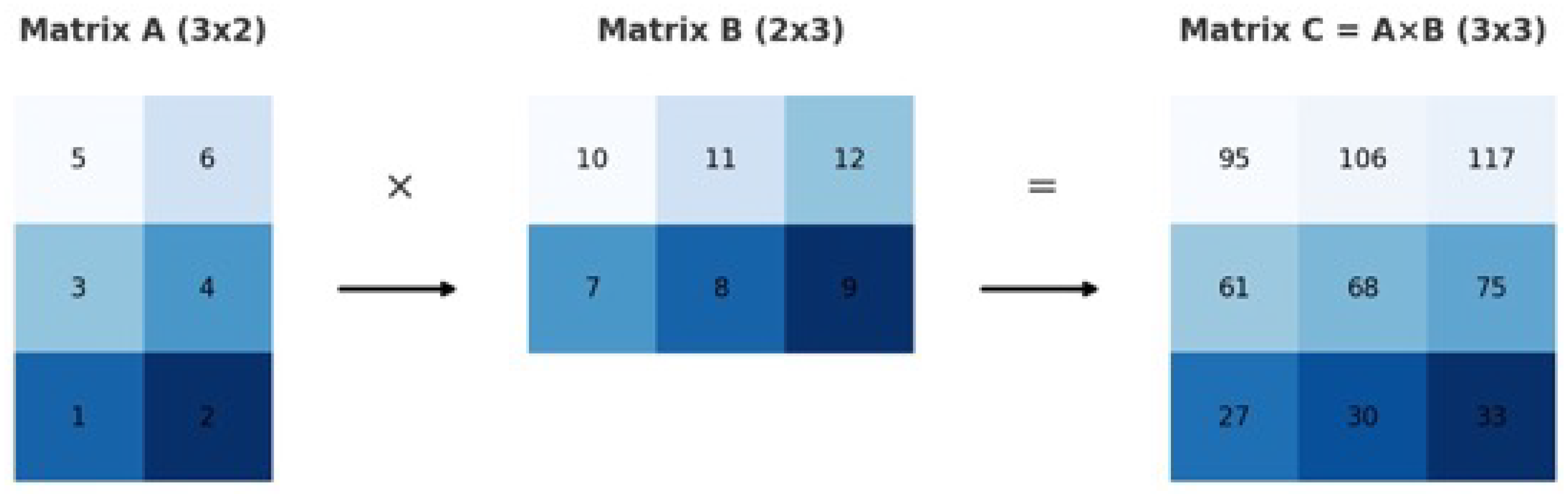
Figure 5.
Example of Matrix Multiplication.
The ability to seamlessly transition between tensorial representations and scalar summaries is foundational for both the theoretical formulation and the practical implementation of Machine Learning systems.
8.12. Matrix Multiplication
Matrix multiplication constitutes one of the more computationally intricate operations performed on tensors. In biological systems, such as the human brain, neurons operate in parallel, dynamically adjusting the strengths of their connections to facilitate learning and adaptation. This dynamic behavior can be abstractly modeled in Machine Learning through matrix multiplication (MatMul), enabling the simulation of neural activity in a form amenable to the linear and deterministic processing style of digital computing hardware.
In formal terms, matrix multiplication involves the systematic combination of two matrices by multiplying corresponding elements and summing the results across aligned dimensions. Crucially, for matrix multiplication to be well-defined, the number of columns in the first matrix must equal the number of rows in the second matrix. Furthermore, efficient computation of matrix multiplication relies on optimized access patterns to large, contiguous sections of memory, underscoring its centrality to both the mathematical formulation and the hardware acceleration of Machine Learning algorithms.
| Listing 8. Formulaic Pythonic Pseudocode for Matrix Multiplication. |
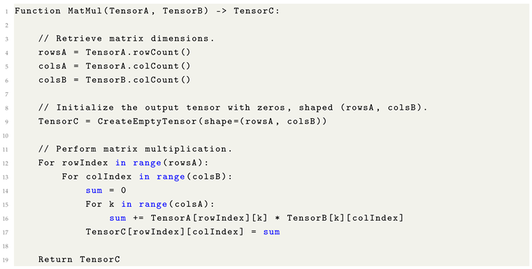 |
It is important to note that the index k represents the shared dimension between the two matrices being multiplied. During the matrix multiplication process, k iterates over the corresponding elements of the first matrix’s row and the second matrix’s column, accumulating their products to compute each element of the resulting matrix. This structure constitutes the fundamental dot product operation underlying matrix multiplication and is critical for enabling efficient linear parallelization in modern computational implementations.
8.12.1. Misconception: Matrix Division?
There is no Matrix Division, while Scalars could apply division to a whole Tensor, a Matrix applyig division, is not a defined general operation. As reverse transformations is too computational expansive.
8.13. Broadcasting
Broadcasting is a fundamental mechanism that enables element-wise operations between tensors of differing shapes by automatically expanding their dimensions to achieve compatibility. The Tensor Broadcasting Rules formally define the conditions under which such expansions are permissible, ensuring that operations can be applied without explicit replication of data.
By adhering to these rules, Machine Learning frameworks can efficiently perform arithmetic operations across tensors of varying ranks and shapes, facilitating flexible model design and reducing computational overhead.
- Broadcasting Rules for Two-Dimensional Tensors:
- Let Tensor A and Tensor B be the two tensors involved in the operation.
- Broadcasting is permissible along the row dimension if the number of rows in A equals the number of rows in B, or if one of the tensors has exactly one row.
- Broadcasting is permissible along the column dimension if the number of columns in A equals the number of columns in B, or if one of the tensors has exactly one column.
- If either the row or column dimension is 1 in one tensor, it is virtually expanded (broadcast) to match the corresponding dimension of the other tensor.
In basic terms, if a tensor dimension equals one, it can be broadcast by expanding that dimension to match the corresponding dimension of the other tensor. However, if the dimensions are neither equal nor one, additional techniques must be employed to achieve shape compatibility. These techniques include zero-padding, reshaping, unsqueezing, and transposition, each of which modifies the tensor’s structure to enable valid operations.
| Listing 9. Formulaic Pythonic Code for Tensor Subtraction. |
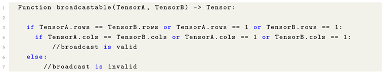 |
Figure 6.
Example of correct broadcasting.
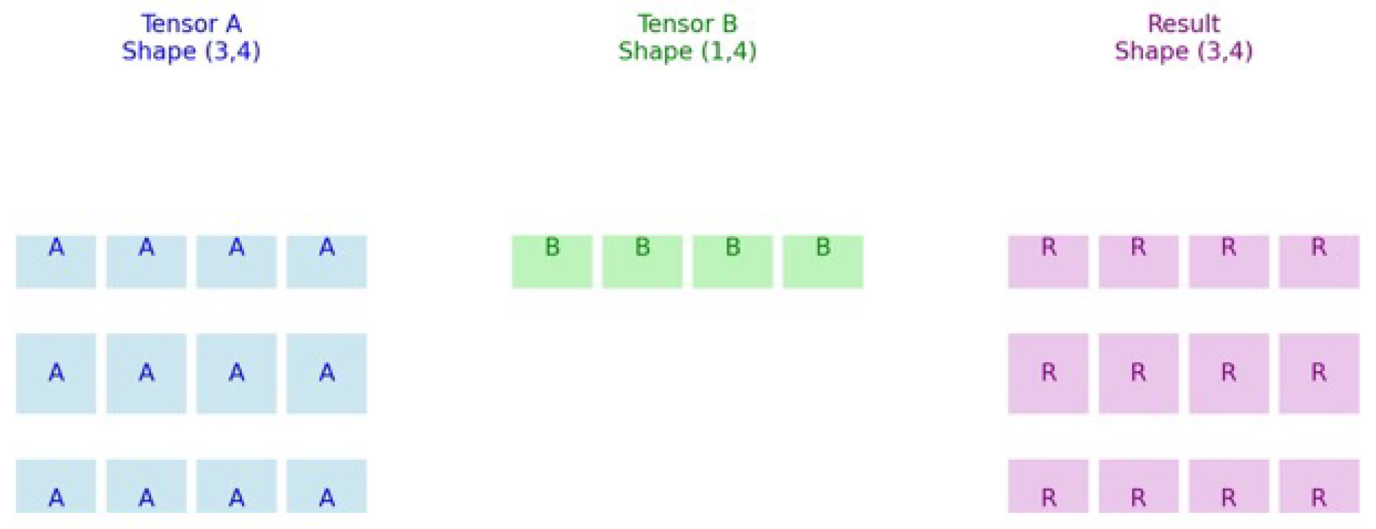
This verification step is particularly critical for matrix multiplication, as the shapes of the input tensors must either be inherently compatible or made compatible through broadcasting in order for the operation to be correctly applied.
8.14. Tensor Raised to a Scalar Power
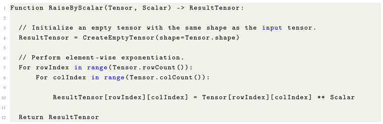
Raising a tensor to a scalar power constitutes an element-wise operation, wherein each individual element of the tensor is exponentiated independently by the scalar value. Unlike matrix multiplication, this operation does not involve any interaction between different elements or dimensions; each computation is performed locally at the element level.
| Listing 10. Formulaic Pythonic Pseudocode for Element-wise Tensor Exponentiation. |
 |
8.14.1. Use Cases
- Activation Functions: Certain activation functions involve raising tensor elements to a scalar power, particularly in custom or experimentally-derived non-linearities.
- Regularization: Element-wise exponentiation can be employed as part of regularization strategies to control model complexity and mitigate overfitting.
- Normalization Techniques: Several normalization methods involve squaring tensor elements, such as in variance normalization or RMS (Root Mean Square) computations.
- Probability Distributions: In probabilistic modeling, tensor elements are often raised to powers when computing likelihoods, especially in formulations involving exponential families or in certain Bayesian inference procedures.
8.14.2. Important Notes
- Element-wise Application: Exponentiation by a scalar applies strictly in an element-wise manner. It does not constitute matrix multiplication, even if the tensor is two-dimensional.
- Scalar Flexibility: The scalar exponent can be any real number, including negative values and fractions, provided that the base tensor elements support the operation (e.g., non-negative bases for real-valued outputs when using fractional exponents).
- Differentiability: Element-wise exponentiation is differentiable almost everywhere and is thus suitable for use in gradient-based optimization algorithms.
- Numerical Stability: The use of non-integer scalars in combination with zero or negative tensor elements may lead to undefined or unstable results, depending on the specific computational context.
- Nonlinear Transformation: Raising tensor elements to a scalar power constitutes a nonlinear transformation, significantly altering the data distribution and affecting downstream computations.
Figure 7.
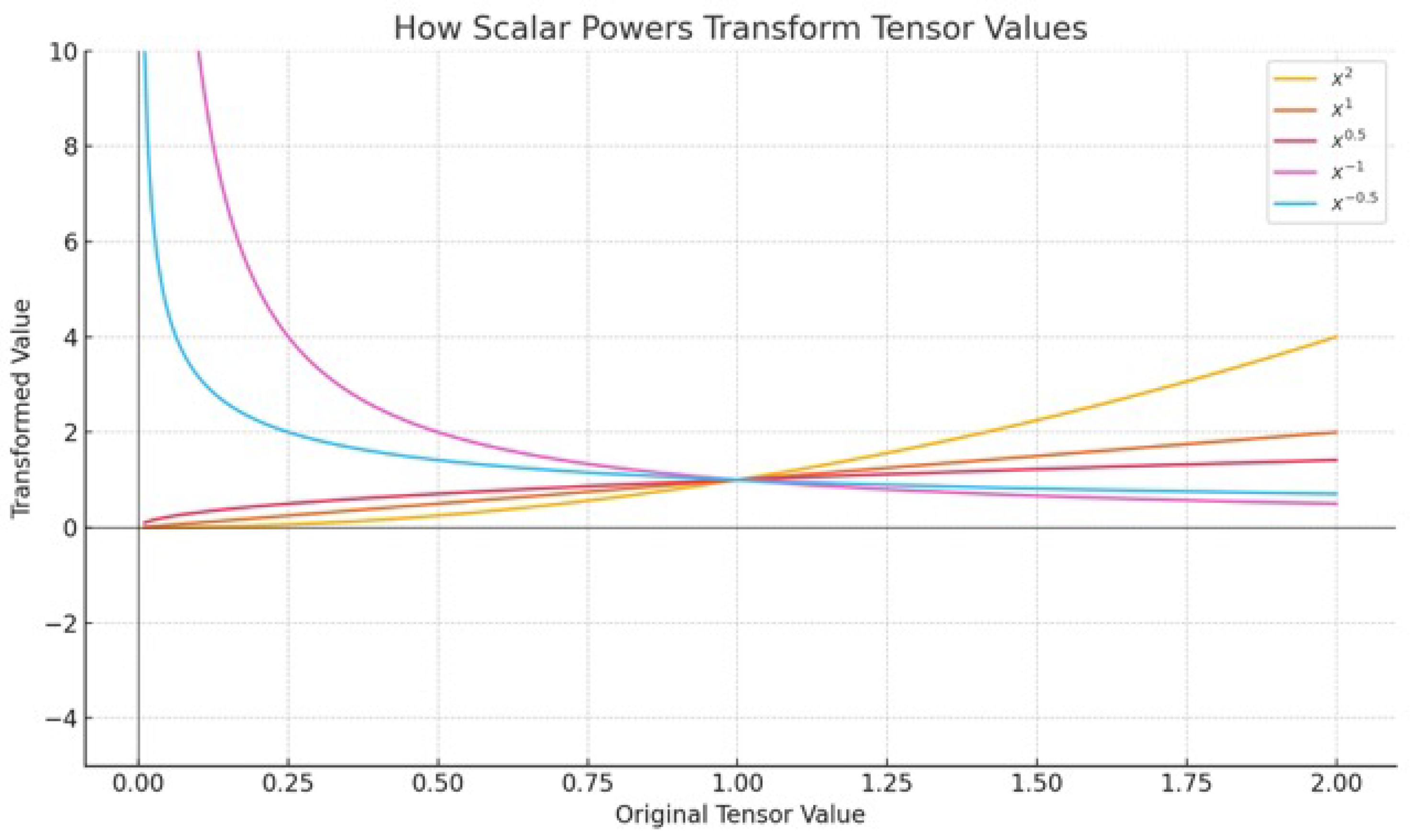
Illustration of how scalar exponentiation transforms tensor values in a non-linear fashion. The graph plots several power operations—specifically , , , , and —applied to an original input range of . While the linear function preserves proportionality, the other transformations introduce significant non-linear distortions: quadratic () expands larger magnitudes, square root () compresses them, and negative powers (, ) produce inverse relationships with rapid growth near zero. This behavior emphasizes that scalar exponentiation inherently constitutes a non-linear operation, often introducing asymmetries, discontinuities, or sensitivity to small inputs within tensor transformations.
Figure 7.
Illustration of how scalar exponentiation transforms tensor values in a non-linear fashion. The graph plots several power operations—specifically , , , , and —applied to an original input range of . While the linear function preserves proportionality, the other transformations introduce significant non-linear distortions: quadratic () expands larger magnitudes, square root () compresses them, and negative powers (, ) produce inverse relationships with rapid growth near zero. This behavior emphasizes that scalar exponentiation inherently constitutes a non-linear operation, often introducing asymmetries, discontinuities, or sensitivity to small inputs within tensor transformations.
9. Tensor Shaping and Broadcasting Operations
In Machine Learning, tensors frequently require structural transformations to ensure compatibility with model architectures. This section presents key tensor shaping and broadcasting operations that facilitate seamless data flow across different layers and model components, while preserving the integrity of the underlying data representations.
9.1. Transpose
The transpose operation enables tensors of differing shapes to achieve matrix-wise compatibility, particularly in contexts where broadcasting is insufficient. Transposition reorients a tensor by swapping its dimensions, effectively rotating the structure to align with the dimensional requirements of another tensor.
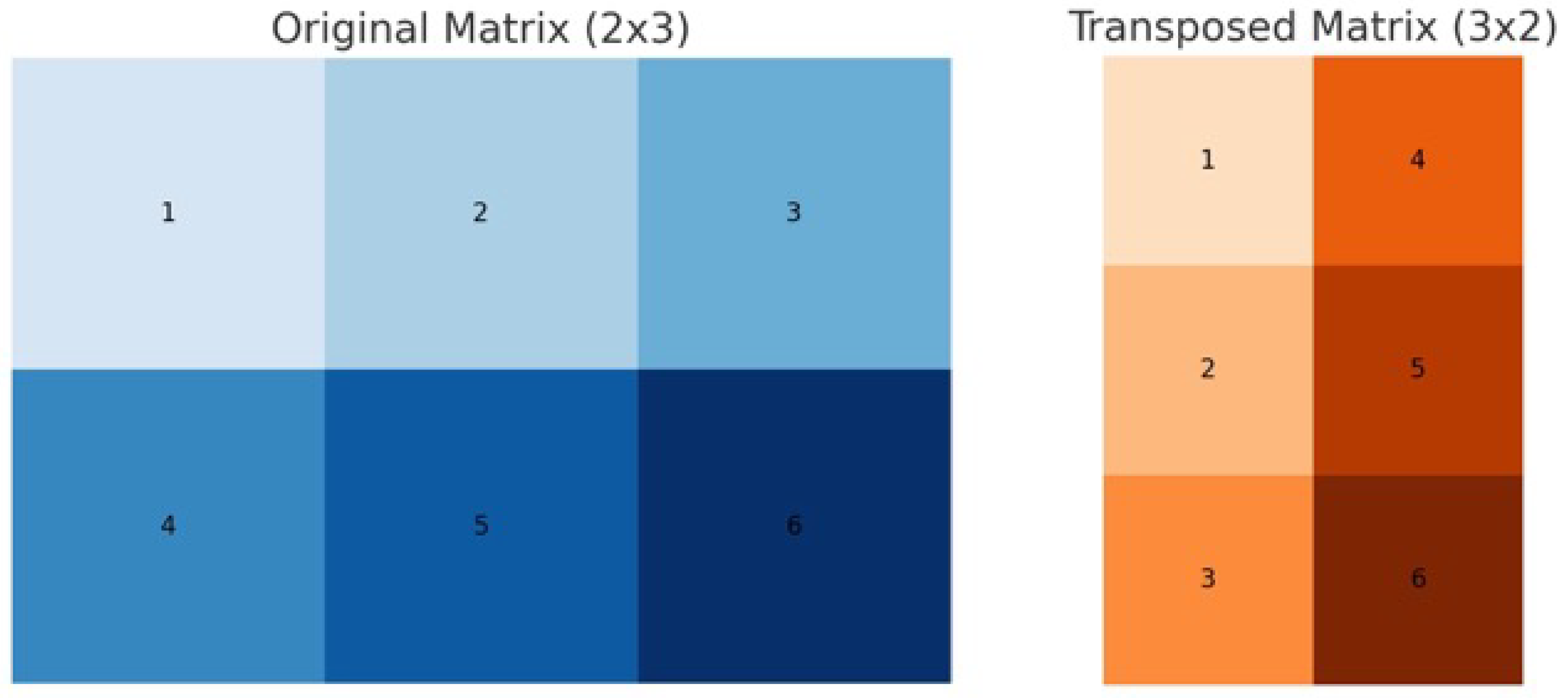
For example, a tensor with shape (5,1) can be transposed to shape (1,5), facilitating element-wise or matrix operations with tensors of compatible shapes.
Figure 8.
Diagram of a Tensor with Transposed applied, demonstrating the rotation.
| Listing 11. Formulaic Pythonic Pseudocode for Tensor Transposition. |
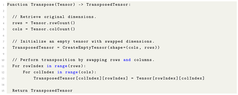 |
This operation is particularly useful for aligning tensor shapes to enable compatibility in operations such as matrix multiplication.
9.2. Padding (Zero Padding)
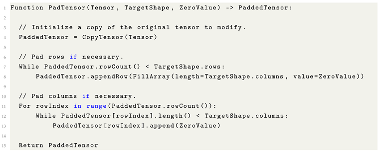
When tensors do not possess the required dimensions for a given operation, padding can be applied to adjust their shapes accordingly. Padding typically operates in two modes: either by appending zero-valued elements to extend rows or columns, or by trimming excess elements to align the tensor with the desired target shape.
Zero padding is particularly common in Machine Learning applications where maintaining spatial or dimensional consistency across layers is critical, such as in convolutional neural networks (CNNs) and structured input pipelines.
| Listing 12. Formulaic Pythonic Pseudocode for Tensor Padding. |
 |
9.3. Flatten
In Machine Learning, particularly within neural network architectures, the flatten operation is used to convert multi-dimensional data structures (e.g., two-dimensional images or three-dimensional feature maps) into a one-dimensional vector.
This transformation is essential because fully connected (dense) layers require one-dimensional input for processing. Flattening serves as a critical bridge between feature extraction layers—such as convolutional or pooling layers—and subsequent classification or output layers, enabling the network to transition from complex spatial representations to scalar predictions or decisions.
| Listing 13. Formulaic Pythonic Pseudocode for Tensor Flattening. |
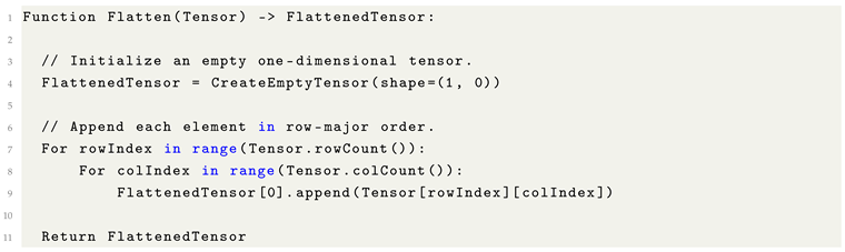 |
Flattening preserves the original element order in a row-major sequence, which is essential for maintaining the structural consistency of features within Machine Learning models.
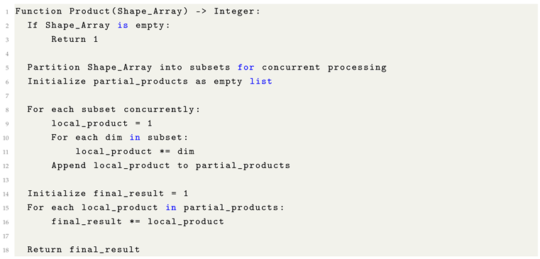
9.4. Dimensional Products
In tensor analysis, the dimensional product corresponds to the total number of discrete elements instantiated within a tensor structure. It is formally derived as the product of the cardinalities along each axis of the tensor’s shape tuple. This invariant is paramount in validating reshape operations, as the conservation of element cardinality is a necessary condition for the consistency and reversibility of tensor transformations.
| Listing 14. Concurrent Formulaic Pythonic Code for Dimensional Product Calculation. |
 |
9.5. Reshape and Resize Operations
During the construction and execution of neural network architectures, it is often encountered that a tensor’s intrinsic shape does not conform to the dimensional requirements of specific operations, notably matrix multiplication and related algebraic transformations. In such instances, it becomes necessary to perform reshape or resize operations, wherein the tensor’s structure is reconfigured to align with the expected dimensionalities of subsequent computational stages. Crucially, these transformations must preserve the total cardinality of the tensor elements, thereby maintaining data integrity while ensuring compatibility across computational layers.
| Listing 15. Concurrent Formulaic Pythonic Code for Tensor Reshape/Resize. |
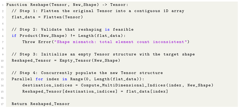 |
Reshape operations reconfigure the memory layout of tensors while preserving the total cardinality of elements. Crucially, reshaping is a valid and safe transformation only when the product of the target dimensions exactly equals the original tensor’s element count. Failure to satisfy this invariant results in structural inconsistency and must be guarded against to avoid runtime violations. Concurrent reshape implementations utilize independent index mappings to facilitate parallel population of the target tensor without contention.
10. Fundamental Mathematical Concepts for Machine Learning
A common misconception among aspiring practitioners is that effective engagement with Machine Learning (ML) requires a comprehensive background in advanced calculus or higher mathematics. While such knowledge may enrich one’s theoretical understanding, the foundational practices of ML rely primarily on a small subset of core mathematical principles. This section delineates those essential constructs, providing both conceptual clarity and pedagogical accessibility.
10.1. Calculus: A Descriptive Framework, Not a Barrier
Calculus serves as a formal mathematical framework for describing continuous change, and historically underpins the derivation of many algorithmic foundations in Machine Learning, including gradient descent, optimization, and activation dynamics. In essence, it provides the language in which many core ML operations were originally formulated. However, for practical implementation, these expressions are routinely translated into discrete algorithmic procedures—what we term *formulaic pseudocode*—rendering deep calculus fluency unnecessary for initial engagement. Practitioners can thus implement state-of-the-art models by understanding the intuition behind derivatives and gradients, even without engaging in symbolic manipulation.
10.2. Non-Linearity: The Essential Break from Linearity
In the context of Machine Learning, non-linearity refers to transformations wherein the output is not a direct proportional mapping of the input. Mathematically, this property manifests in functions whose graphs are not straight lines—such as polynomials, exponentials, or activation functions like ReLU and GELU. The introduction of non-linear transformations within models is critical, as it enables neural networks to approximate complex, non-trivial patterns in high-dimensional data. Without non-linearity, models would be restricted to learning only affine transformations, severely limiting their expressive capacity.
10.3. Euler’s Number: A Fundamental Limit in Continuous Growth
Euler’s number, denoted as , emerges as a foundational constant in both calculus and Machine Learning. It characterizes the asymptotic behavior of processes involving continuous exponential growth and decay, as well as the natural logarithmic base in optimization landscapes. Formally, Euler’s number may be defined as the infinite limit of either a summation or a compounding product. The most common series representation is given by:
This identity expresses e as the sum of the reciprocals of factorials—a rapidly converging series foundational to both exponential function approximations and gradient-based methods involving activation functions such as softmax.
The following pseudocode outlines an iterative approach to approximate e using its factorial series expansion:
| Listing 16. Formulaic Pythonic Code for Euler’s Number Approximation. |
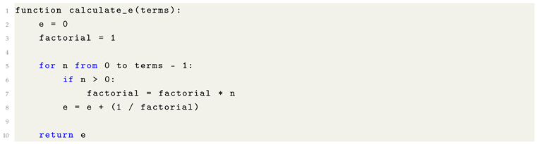 |
Most modern programming languages provide Euler’s number as a built-in constant within their standard mathematical libraries (e.g., math.e in Python, std::numbers::e in C++20). However, explicit calculation via factorial expansion serves as a valuable pedagogical exercise for understanding its convergence behavior and underlying mathematical structure.
10.4. Mean of a Tensor: A Measure of Central Tendency
In Machine Learning, the mean—or arithmetic average—of a tensor’s elements provides a fundamental measure of central tendency. This scalar value summarizes the overall distribution of the data and is frequently employed in normalization schemes, statistical analyses, and loss function diagnostics. For a tensor , the mean is defined as:
where denotes the total number of elements in the tensor, and represents the i-th flattened element.
The operation is both commutative and associative, enabling safe concurrent or parallelized computation. The following pseudocode illustrates a basic implementation:
| Listing 17. Formulaic Pythonic Code for Tensor Mean. |
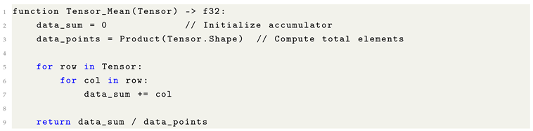 |
In practice, most numerical computing libraries (e.g., NumPy, TensorFlow, PyTorch) provide optimized implementations that support high-dimensional tensors and exploit vectorized operations or GPU acceleration. Nevertheless, the explicit formulation serves as an instructive model for understanding the mechanics of aggregation in tensor algebra.
10.5. Median of a Tensor: A Robust Measure of Central Tendency
In statistical analysis of tensor data, the median serves as a robust estimator of central tendency, particularly effective in scenarios involving skewed distributions or the presence of outliers. Unlike the mean, which aggregates all values and may be influenced by extreme values, the median captures the central value of the dataset after ordering the elements by magnitude.
Formally, given a tensor T of arbitrary rank with n total elements, the median is defined by first flattening the tensor into a one-dimensional array and then sorting its entries in non-decreasing order. The median value m is then determined as follows:
where denotes the i-th smallest element in the sorted array.
This procedure ensures that 50% of the data lies below and above the computed median. The median is particularly advantageous in Machine Learning workflows for tasks such as feature scaling, distributional normalization, and robust data imputation.
| Listing 18. Formulaic Pythonic Code for Tensor Median. |
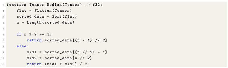 |
While computationally more expensive than the mean, the median offers resilience against noisy data and extreme values, making it a preferred choice in adversarial or corrupted input environments. Optimized implementations often leverage partial sorting or selection algorithms (e.g., QuickSelect) to achieve linear-time complexity in practice.
10.6. Element-wise Absolute Value of a Tensor
The element-wise absolute value operation is a fundamental transformation in numerical computing and Machine Learning, frequently employed in contexts such as error computation, signal processing, and gradient stabilization. For a given tensor , the absolute value operator is defined as:
where denotes the scalar absolute value. This operation ensures that all resulting elements are non-negative, as it transforms each negative entry into its positive counterpart while preserving non-negative values.
In vectorized frameworks, this transformation is typically applied in a fully parallelized manner, operating independently on each tensor element. Its utility spans across applications such as the L1 norm, absolute error metrics (e.g., MAE), and robust loss functions that penalize deviations symmetrically regardless of sign.
| Listing 19. Formulaic Pythonic Code for Element-wise Tensor Absolute Value. |
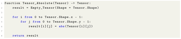 |
Most high-performance libraries provide optimized implementations of this operation using SIMD instructions or GPU kernels. Nonetheless, the conceptual clarity of the element-wise absolute function makes it a foundational operation in both algorithm design and educational formulations.
10.7. Tensor Standard Deviation (std): A Measure of Dispersion
The standard deviation is a fundamental statistical metric used to quantify the dispersion or spread of data relative to its mean. Within the context of Machine Learning, computing the standard deviation of a tensor is essential for normalization techniques, statistical diagnostics, and sensitivity analysis in gradient-based optimization.
Formally, given a tensor T of n elements, with mean , the population standard deviation is defined as:
In practice, the sample standard deviation may be used instead, where the denominator is to provide an unbiased estimator of variance when working with sample data:
The standard deviation thus captures the average magnitude of deviation from the mean and provides insight into the distributional shape of tensor values.
The following pseudocode outlines a generalized computation of standard deviation for a flattened tensor:
| Listing 20. Formulaic Pythonic Code for Tensor Standard Deviation. |
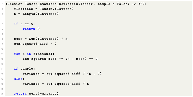 |
This operation is numerically stable and can be parallelized across elements, particularly when computing in GPU-accelerated environments. Most tensor libraries (e.g., PyTorch, TensorFlow, NumPy) offer optimized implementations that leverage fused operations to compute the mean and variance with minimal passes over memory.
10.8. Hyperparameters: Configurable Variables in Model Design and Optimization
In the architecture and training of Machine Learning models, hyperparameters are external configuration variables whose values are not learned from data but are instead set prior to the training process. These values govern both the structural properties of the model and the dynamics of the optimization procedure. Unlike parameters (e.g., weights and biases), which are optimized via backpropagation, hyperparameters are tuned manually or through meta-optimization strategies.
Hyperparameters can be broadly classified into the following categories:
-
(1) Model Architecture Hyperparameters define the structural configuration of the neural network:
- Number of layers: The depth of the network, affecting its representational capacity.
- Neurons per layer: The dimensionality of each transformation, controlling expressive power.
- Activation functions: Non-linear transformations (e.g., ReLU, Sigmoid, GELU) applied to neurons, introducing model non-linearity.
-
(2) Optimization Hyperparameters govern how the model is trained using gradient descent:
- Learning rate: The step size at each iteration of optimization; critical for convergence behavior.
- Batch size: Number of training samples processed per update; affects memory usage and gradient stability.
- Epochs: The number of complete passes over the training dataset.
- Optimizer: Algorithm used to update weights (e.g., SGD, Adam, RMSProp), each with its own internal dynamics.
-
(3) Regularization Hyperparameters mitigate overfitting and improve generalization:
- Dropout rate: Fraction of neurons randomly deactivated during training to prevent co-adaptation.
- L1/L2 regularization coefficients: Penalize large weights to encourage sparsity or smoothness.
- Non-linearity inclusion: The use of activation functions contributes indirectly to regularization by introducing model flexibility.
-
(4) Hyperparameter Tuning Strategies determine how hyperparameters are selected:
- Grid search: Exhaustive evaluation across a Cartesian product of predefined hyperparameter values.
- Random search: Random sampling from defined distributions over hyperparameter values.
- Bayesian optimization: Model-based approach that builds a probabilistic surrogate function to efficiently explore the search space.
- Advanced methods: Includes algorithms like Hyperband, Optuna, and Population-Based Training (PBT) for scalable and adaptive tuning.
Hyperparameter tuning remains a central component of model performance optimization and generalization. Automated hyperparameter search frameworks are increasingly integrated into modern ML workflows to streamline this process while balancing exploration and computational cost.
10.9. Function Hyperparameters: Tunable Modifiers of Algorithmic Behavior
In the formulation of many mathematical functions used within Machine Learning algorithms, certain parameters—termed function hyperparameters—are introduced to modulate the function’s internal dynamics. These hyperparameters are not learned from data, but are manually specified or tuned to adapt the function’s behavior to the characteristics of a given task.
Function hyperparameters often control properties such as smoothing, weighting, or curvature, and are integral to operations including optimization, regularization, and activation. Although many such functions provide empirically derived default values, adjusting these hyperparameters can significantly impact model convergence, performance, and stability.
- Example: Exponential Moving Averages in the Adam Optimizer
The Adam optimizer, widely used for stochastic gradient-based training, maintains exponential moving averages of past gradients and squared gradients. It introduces two key hyperparameters:
- Beta1 controls the decay rate of the moving average of the first moment (gradient). A typical default is , meaning recent gradients are weighted more heavily than earlier ones.
- Beta2 governs the second moment (squared gradients), often set to to ensure long-term memory of variance.
These hyperparameters effectively shape the optimizer’s sensitivity to recent versus historical gradient information, influencing convergence speed and stability. Improper tuning can lead to oscillation or stagnation, particularly in the presence of noisy gradients or sparse features.
Function hyperparameters appear across the Machine Learning pipeline, including:
- Dropout rate in regularization functions
- Alpha in leaky ReLU or ELU activations
- Temperature in softmax-based sampling
- Kernel width in Gaussian functions or RBF kernels
Understanding and tuning these hyperparameters is crucial for aligning theoretical function behavior with empirical model dynamics.
10.10. Derivatives: Quantifying Change in Continuous Functions
The derivative is a foundational concept in calculus that quantifies the instantaneous rate of change of a function with respect to one of its input variables. In the context of Machine Learning, derivatives are central to optimization procedures such as gradient descent, where model parameters are iteratively updated based on the slope of the loss function.
Formally, the derivative of a scalar-valued function with respect to its input x is defined as the limit:
This expression captures the rate at which changes as x varies, and provides the tangent slope of the function at a given point. For differentiable functions, this allows local linear approximations and facilitates analytical optimization.
- Example: Power Function Derivative
Consider the function:
Its derivative, computed using standard calculus rules, is:
This indicates that the rate of change of the function at any point x is proportional to x itself. Evaluating the derivative at , we obtain:
Thus, at , the function is increasing at a rate of 6 units for every unit increase in x.
In Machine Learning, derivatives are used to compute gradients—vector-valued generalizations of partial derivatives across multivariate functions—which are instrumental in parameter updates. The efficient computation of such derivatives, often via automatic differentiation, is critical to the scalability of modern deep learning frameworks.
10.11. Epsilon (): Thresholds for Numerical Stability and Convergence
In numerical analysis and Machine Learning algorithms, the symbol (epsilon) conventionally denotes a small positive quantity used as a threshold for precision, stability, or convergence criteria. Unlike dynamic variables or learned parameters, epsilon is a manually specified hyperparameter that defines tolerable bounds for terminating iterative procedures or preventing division-by-zero instabilities.
Formally, in optimization algorithms such as gradient descent, an iteration may be halted once the magnitude of the gradient norm falls below a predefined threshold , indicating that further progress is negligible:
Similarly, in algorithms involving floating-point divisions, epsilon is often added to denominators to avoid undefined behavior:
- Illustrative Example: Iterative Stopping Criterion
Consider an iterative optimization algorithm where updates continue until:
This ensures that the relative change between successive iterations is sufficiently small, implying convergence to a (local) optimum within acceptable tolerance.
- Important Clarification
Epsilon () should not be confused with Euler’s number (), which is a mathematical constant describing natural exponential growth. While e is fundamental to continuous mathematical modeling, serves as a practical device for managing numerical precision and algorithmic termination.
10.12. Geometric Symbols and Mathematical Constants in Machine Learning
Mathematical constants and geometric symbols play critical yet often understated roles in the formulation and analysis of Machine Learning algorithms. Although some constants, such as , are more prominent in pure mathematics and physics, they appear in subtle yet essential ways within statistical modeling, optimization theory, and loss function derivations.
- (1) The Constant
The constant arises primarily in Machine Learning through its connections to probability theory, particularly in the context of continuous probability distributions. For instance, the probability density function of the normal (Gaussian) distribution involves explicitly:
Here, ensures proper normalization of the distribution such that the total probability integrates to one. Applications of Gaussian distributions are ubiquitous in Machine Learning, including modeling noise, regularization (e.g., Gaussian priors), and understanding loss landscapes in stochastic optimization.
Moreover, occasionally appears in more advanced operations involving Fourier analysis, kernel methods, and information theory metrics, albeit less frequently than constants like e.
- (2) The Constant e
Euler’s number is far more central to Machine Learning, underpinning exponential functions, logarithmic transformations, and the softmax function. e governs the behavior of probability distributions, learning rate decays, and loss formulations involving cross-entropy.
- (3) The Symbol
The Greek letter is widely used to denote model parameters, particularly in optimization and learning contexts. Conceptually, may represent:
- The parameter vector in linear models (e.g., in logistic regression, encapsulates weights and biases).
- The orientation or slope of a function with respect to its gradient during optimization.
In gradient-based methods such as Adam, SGD, or RMSprop, evolves iteratively via update rules of the form:
where denotes the learning rate and the loss function. Here, the gradient provides the direction and rate of steepest ascent, and updates to occur in the opposite direction to minimize loss.
While originally symbolizes angular quantities in geometry and trigonometry, its usage in Machine Learning reflects a broader abstraction: the idea of navigating parameter spaces and controlling optimization trajectories.
In summary, geometric constants and symbols, although sometimes subtle in appearance, are deeply embedded within the theoretical infrastructure of modern Machine Learning. Their understanding facilitates deeper insights into algorithmic behavior, statistical assumptions, and optimization landscapes.
10.13. The Error Function (): A Fundamental Link to Gaussian Distributions
The error function, denoted as , is a special function of fundamental importance in probability theory, numerical analysis, and Machine Learning. It quantifies the probability that a random variable from a standard normal distribution falls within a given symmetric interval around the mean.
Formally, the error function is defined as:
This expression describes the normalized integral of the Gaussian function from 0 to x, scaled appropriately to map asymptotically to as x tends toward .
- Applications in Machine Learning
The function arises in several contexts within Machine Learning and related disciplines:
- Activation functions: The Gaussian Error Linear Unit (GELU) activation function, used prominently in Transformer architectures, incorporates for smooth non-linear transformations.
- Optimization algorithms: Some adaptive optimizers and smoothing functions leverage for stabilizing updates or defining soft thresholds.
- Probabilistic modeling: In Gaussian processes, diffusion models, and statistical physics-inspired ML methods, naturally emerges due to its relation to cumulative Gaussian distributions.
- Numerical Approximation
Given that the error function has no closed-form expression in terms of elementary functions, numerical approximations are often employed. The following pseudocode illustrates a basic numerical integration approach using the trapezoidal rule:
| Listing 21. Formulaic Pythonic Code for Numerical Approximation of erf. |
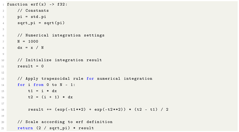 |
Most modern programming environments, such as Python (math.erf), C++ (std::erf), and numerical libraries (e.g., SciPy), provide highly optimized native implementations of the error function. When available, these should be preferred for computational efficiency and numerical stability.
11. Activation Functions: Modeling Complex Neuronal Dynamics
11.1. Meaning of Activation
In the context of artificial neural networks, an activation refers to the output response of a neuron given its input signal. Conceptually, it quantifies the extent to which a neuron “fires” based on the strength and characteristics of incoming information. Mathematically, activation functions determine whether a neuron transmits its signal onward within the network architecture.
11.2. Purpose and Biological Motivation
Biological neurons are interconnected through synapses—specialized junctions where chemical and electrical signals determine whether the post-synaptic neuron becomes activated. The decision to fire is influenced not only by the magnitude of incoming signals but also by complex, nonlinear biochemical processes occurring within the synaptic cleft.
Simulating these intricate processes at a molecular level is computationally intractable for large-scale models. Consequently, artificial neural networks approximate neuronal dynamics through the use of mathematically defined activation functions. These functions capture the essence of biological activation by introducing nonlinear transformations that allow networks to approximate complex, high-dimensional mappings between inputs and outputs.
- Mathematical Role of Activation Functions
Activation functions serve two primary roles:
- Non-linearity introduction: Without non-linear activations, a network composed solely of affine transformations (matrix multiplications and bias additions) would collapse into a single equivalent linear transformation, severely limiting representational capacity. Non-linear activations (e.g., ReLU, sigmoid, GELU) enable networks to approximate arbitrary continuous functions, a property formally guaranteed by the Universal Approximation Theorem.
- Information shaping: Activations modulate the flow of information through the network layers, allowing selective amplification, suppression, or transformation of learned features. This shaping mechanism is crucial for the emergence of hierarchical feature representations in deep architectures.
Thus, activation functions are indispensable both biologically and computationally. They enable artificial systems to mirror key principles of biological cognition while simultaneously expanding their mathematical expressive power beyond that of simple linear models.
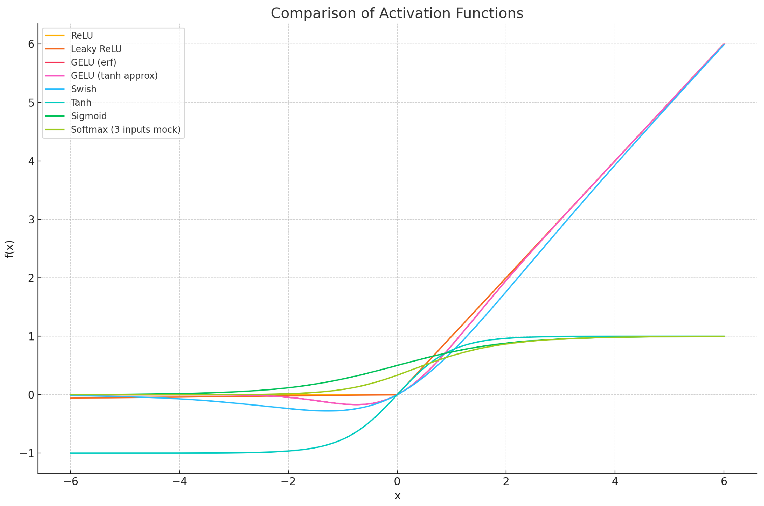
Figure 9.
Comparison of common activation functions (ReLU, Leaky ReLU, GELU, Swish, Tanh, Sigmoid, Softmax).
Figure 9.
Comparison of common activation functions (ReLU, Leaky ReLU, GELU, Swish, Tanh, Sigmoid, Softmax).
11.3. Activation Function Progression and Comparative Analysis
The selection and ordering of activation functions in this section is designed to introduce increasingly sophisticated transformations, beginning with foundational piecewise-linear functions and progressing toward smooth, probabilistic activations optimized for modern deep learning architectures. The sequence culminates with the Gaussian Error Linear Unit (GELU), widely adopted in Transformer-based models.
11.3.1. Comparative Overview of Activation Functions

Table 1.
Summary Comparison of Activation Functions.
| Activation | Range | Non-linearity | Key Notes |
|---|---|---|---|
| ReLU | Sharp | Simple, sparse activation; efficient for deep convolutional networks. | |
| Leaky ReLU | Sharp | Introduces a small negative slope to address neuron inactivity. | |
| Swish | Smooth | Self-gating; improves performance, especially in very deep networks. | |
| GELU (erf) | Smooth | Probabilistic activation; superior performance in Transformer architectures. | |
| tanh | Smooth | Zero-centered; common in recurrent neural networks. | |
| GELU (tanh) | Smooth | Computationally efficient approximation of GELU. |
11.3.2. Expanded Insights on Activation Functions
Table 2.
Detailed Observations on Activation Functions.
| Activation | Additional Insights |
|---|---|
| ReLU | Prone to the “dying ReLU” phenomenon, where neurons output zero for all inputs. Dominant in CNNs due to computational simplicity. |
| Leaky ReLU | Commonly uses a negative slope coefficient ; mitigates dying neuron problems without introducing significant complexity. |
| Swish | Developed by Google researchers; exhibits non-monotonicity, enabling richer feature representations. |
| GELU (erf) | Softly gates inputs based on magnitude; combines ReLU’s sparsity with smoothness near the origin. |
| tanh | Saturates at the extremes, leading to vanishing gradients; more stable than sigmoid for zero-centered outputs. |
| GELU (tanh) | Provides a near-equivalent functional behavior to GELU with reduced computational overhead. |
11.3.3. Practical Tips and Cautions
Table 3.
Practical Guidelines for Activation Function Selection.
| Activation | Usage Tips and Warnings |
|---|---|
| ReLU | Recommended as a default; monitor for neuron death, especially under aggressive learning rates. |
| Leaky ReLU | Useful when ReLU leads to stagnant training; helps maintain gradient flow even for negative inputs. |
| Swish | Yields marginally better performance in deep architectures at the cost of slightly increased computational burden. |
| GELU (erf) | Preferred for Transformer-based architectures (e.g., BERT, GPT) due to its smooth probabilistic gating behavior. |
| tanh | Best suited for recurrent architectures where centered activations improve gradient dynamics. |
| GELU (tanh) | Ideal for hardware-constrained environments seeking GELU-like performance with faster evaluation. |
11.4. Rectified Linear Unit (ReLU): Definition, Properties, and Practical Considerations
11.4.1. Intuitive Overview
The Rectified Linear Unit (ReLU) activation function introduces non-linearity by transforming all negative inputs to zero while preserving positive values. Conceptually, ReLU “filters” input signals, suppressing negative activations and allowing positive signals to propagate. This operation enhances the expressivity of neural networks without introducing significant computational overhead.
11.4.2. Mathematical Definition
Formally, ReLU is defined as an element-wise transformation:
for each input x. This operation is applied independently to each element in the input tensor, requiring no global context or inter-element dependencies.
- Formulaic Pseudocode Implementation:
| Listing 22. Formulaic Pythonic Code for ReLU Activation. |
 |
This element-wise independence allows efficient parallelization on modern hardware architectures, such as GPUs and TPUs.
11.4.3. Advantages and Use Cases
ReLU activation is widely adopted in deep learning due to the following properties:
- Introduction of Non-linearity: ReLU introduces non-linear transformations while retaining simplicity.
- Computational Efficiency: It requires only a simple thresholding operation, making it extremely fast to compute.
- Alleviation of Vanishing Gradient Problem: Unlike saturating activations (e.g., sigmoid, tanh), ReLU maintains stronger gradient magnitudes, improving optimization in deep networks.
- Sparsity Induction: ReLU naturally produces sparse activations by zeroing out negative values, reducing the effective computational burden and promoting representational efficiency.
- Positive Constraint: By filtering out negative values, ReLU enforces non-negative activations, which can be advantageous in certain architectures and regularization schemes.
- Faster Convergence: Empirically, networks employing ReLU converge faster during training compared to those using traditional saturating activations.
11.4.4. Limitations and Cautions
Despite its advantages, ReLU presents certain limitations:
- Limited Representational Scope: By entirely discarding negative activations, ReLU can hinder the model’s ability to learn functions where negative outputs are semantically meaningful.
- Dying ReLU Phenomenon: Neurons can become permanently inactive if their inputs consistently yield negative values during training, resulting in zero gradients and loss of learning capacity for those neurons.
- Suitability for Complex Relationships: For highly intricate or symmetric data patterns involving negative domains, alternative activations such as Leaky ReLU, ELU, or GELU may offer superior performance.
11.4.5. Why is it faster to train?
You’re trying to capture a simpler relationship, with a very efficient computation formula.
11.4.6. Alternative for ReLU, Leaky ReLU
- Solves the Negative relationship to keep neurons out of the inactive state.
- Able to calculate a tiny bit more relationships.
Figure 10.
ReLU graphed mainly to show the curve.
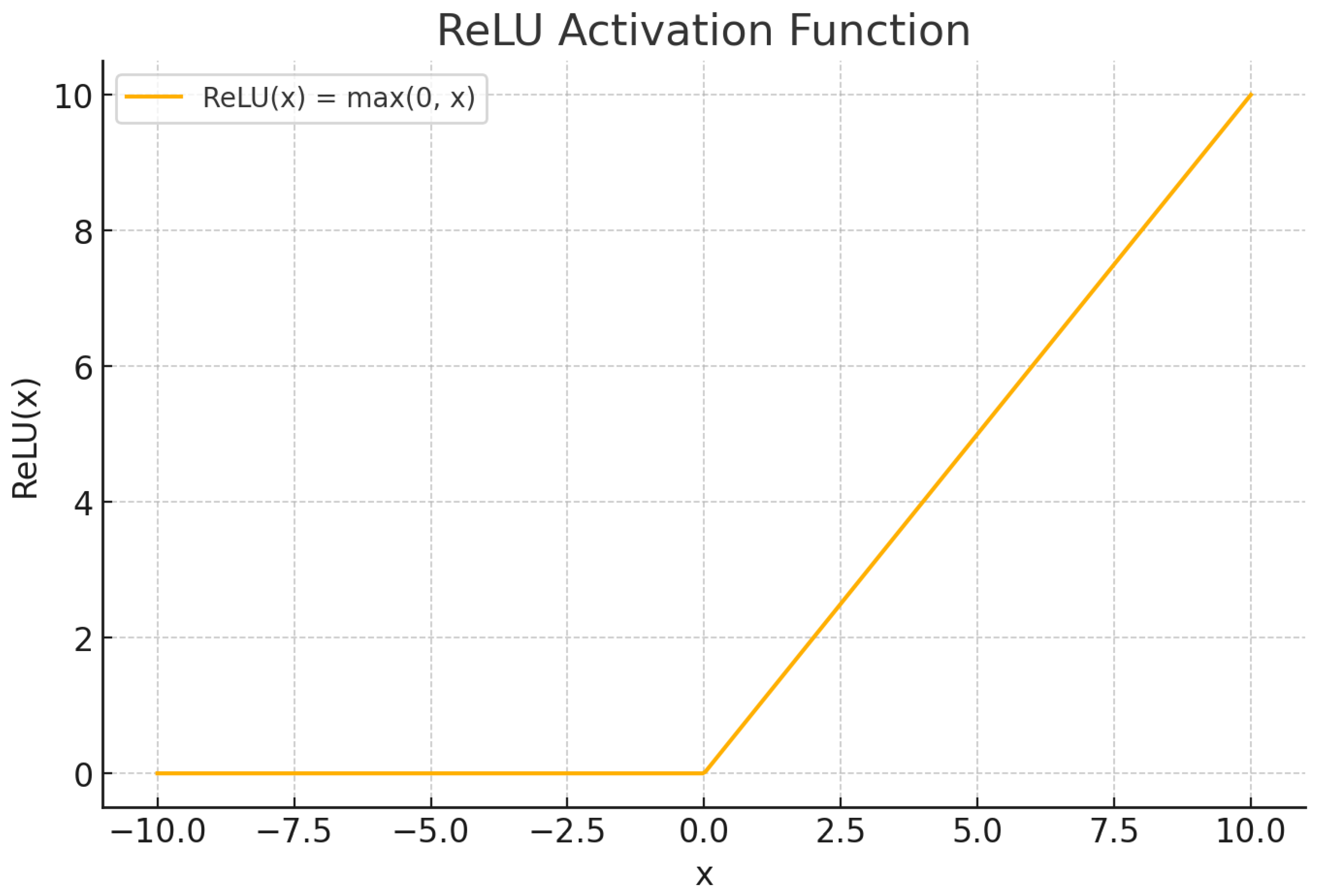
11.4.7. ReLU graph
Notice how the graph remains flat and then abruptly shifts at a sharp angle. This discontinuity in slope is a hallmark of a non-smooth function. For example, ReLU exhibits this behavior with a sharp kink at zero. In contrast, smooth activation functions like GELU produce a more gradual polynomial-like curve with continuous derivatives. This smoothness allows the model to capture more nuanced patterns and learn more complex relationships in data, whereas non-smooth functions may limit expressiveness in certain cases.
- Slope, less than 0 region: Remain at 0
- Slope, greater than 0 region: Regular linear increase
11.5. Leaky Rectified Linear Unit (Leaky ReLU, LReLU): Definition, Properties, and Applications
11.5.1. Intuitive Overview
The Leaky Rectified Linear Unit (Leaky ReLU or LReLU) extends the standard ReLU activation by allowing a small, non-zero gradient when the input is negative. Instead of mapping all negative values to zero, LReLU scales them by a small constant factor, thereby maintaining a minimal signal flow even for negative activations.
11.5.2. Mathematical Definition
Formally, the Leaky ReLU function is defined as:
where is a small positive hyperparameter (commonly set to ) that controls the slope for negative inputs.
11.5.3. Formulaic Pseudocode Implementation
| Listing 23. Formulaic Pythonic Code for Leaky ReLU Activation. |
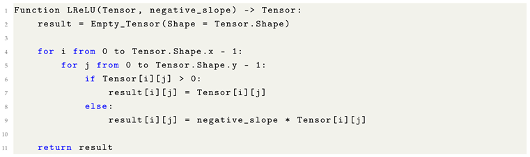 |
Like ReLU, LReLU is an element-wise operation, enabling efficient parallelization on modern hardware architectures.
11.5.4. Advantages and Use Cases
Leaky ReLU offers several practical benefits:
- Introduction of Non-linearity: Similar to ReLU, LReLU introduces essential non-linear transformations into the network.
- Mitigation of Vanishing Gradients: By maintaining a non-zero gradient for negative inputs, LReLU reduces the risk of gradient vanishing compared to saturating functions like sigmoid or tanh.
- Neuron Survival: Allows neurons to maintain small gradients even when weights initially result in negative pre-activations, preventing complete neuron inactivity ("dying ReLU" problem).
- Efficient Computation: Simple to implement and computationally inexpensive, making it suitable for real-time or resource-constrained applications.
- Improved Convergence Speed: Networks employing LReLU often converge faster than those using pure ReLU in scenarios where data distributions produce many negative activations.
- Alternative to ReLU in Hidden Layers: Particularly beneficial in architectures where ReLU leads to excessive neuron death or sparse representations become detrimental.
11.5.5. Limitations and Cautions
Despite its improvements over ReLU, LReLU presents specific limitations:
- Limited Expressivity for Complex Patterns: While suitable for basic feature extraction, LReLU may not sufficiently capture highly intricate or symmetric relationships that require more sophisticated activations.
- Retention of Negative Values: Although small, the leakage of negative signals may not always align with tasks that benefit from strict non-negative representations.
11.5.6. Training Efficiency Considerations
LReLU accelerates training primarily by preserving gradient flow throughout the network, even when activations are negative. This ensures that learning signals are not entirely extinguished, facilitating more stable and faster convergence compared to ReLU in challenging data regimes.
11.5.7. Graphical Interpretation of Leaky ReLU
As illustrated in Figure 11, the behavior of LReLU can be characterized as:
- Negative Region: For inputs , the function exhibits a slight downward tilt determined by the negative slope , allowing a small gradient (leak) to persist.
- Positive Region: For inputs , the function behaves as a standard identity mapping (), identical to ReLU behavior.
11.6. Swish Activation Function: Definition, Properties, and Practical Considerations
11.6.1. Intuitive Overview
The Swish activation function introduces a smooth, non-monotonic transformation that enhances the representational capacity of neural networks. Unlike ReLU, which abruptly zeroes out negative inputs, Swish softly suppresses negative values without completely discarding them. This property enables networks to learn more nuanced and complex patterns across the input domain.
11.6.2. Mathematical Definition
Formally, the Swish activation function is defined as:
where denotes the sigmoid function:
Thus, the Swish function smoothly gates input values based on their own magnitude, combining linear and non-linear behaviors adaptively.
11.6.3. Formulaic Pseudocode Implementation
| Listing 24. Formulaic Pythonic Code for Swish Activation. |
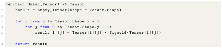 |
The operation is element-wise and inherently parallelizable, making it suitable for large-scale tensor computations.
11.6.4. Advantages and Use Cases
Swish activation offers several compelling properties:
- Non-linearity Introduction: Provides a smooth, non-monotonic mapping that enhances feature expressivity.
- Preservation of Negative Information: Unlike ReLU, Swish retains small negative values, facilitating richer learning dynamics.
- Improved Gradient Flow: The continuous derivative of Swish helps mitigate both vanishing and exploding gradient problems during backpropagation.
- Superior Performance: Empirical studies show that Swish often outperforms ReLU on deep convolutional networks (CNNs), Transformer architectures, and large-scale classification tasks.
- Suitability for Deep Architectures: Particularly effective in very deep models where smooth transitions improve optimization dynamics.
- Alternative to Sigmoid: Provides smoothness without suffering from the severe saturation issues of pure sigmoid activations.
11.6.5. Limitations and Practical Considerations
Despite its advantages, Swish has certain drawbacks:
- Increased Computational Cost: Evaluation of the sigmoid function adds overhead compared to simpler activations like ReLU.
- Training Latency: Networks utilizing Swish may exhibit slower per-epoch training times relative to ReLU.
- Compatibility Limitations: Some machine learning frameworks may not natively support Swish, requiring custom implementation.
- Tradeoff with Simplicity: In some scenarios, the benefits of Swish may be marginal relative to its additional complexity and computational burden.
11.6.6. Graphical Interpretation of Swish
As shown in Figure 12, the behavior of Swish can be characterized as follows:
- Negative Region (): For negative inputs, Swish exhibits a small positive slope, allowing modest signal flow. Unlike ReLU, which zeroes negative inputs, Swish softly attenuates them, preserving some gradient and information flow during training.
- Positive Region (): For positive inputs, Swish behaves increasingly like the identity function, with the slope approaching 1 for large positive values. This ensures that strong activations pass through with minimal distortion, similar to ReLU but with smoother transitions.
11.7. Sigmoid Activation Function: Definition, Properties, and Practical Considerations
11.7.1. Intuitive Overview
The Sigmoid activation function transforms input values into a bounded range between 0 and 1, introducing smooth non-linearity into the network. This mapping is particularly useful for interpreting outputs as probabilities or confidence scores in binary classification tasks. Sigmoid activation ensures that the output is easily interpretable while compressing extreme input values toward asymptotic limits.
11.7.2. Mathematical Definition
Formally, the Sigmoid function is defined as:
where e denotes Euler’s number (). As x tends toward positive infinity, approaches 1; as x tends toward negative infinity, approaches 0. The function is continuous, differentiable, and monotonic.
11.7.3. Formulaic Pseudocode Implementation
| Listing 25. Formulaic Pythonic Code for Sigmoid Activation. |
 |
The Sigmoid operation is element-wise and highly parallelizable, enabling efficient implementation on modern computational hardware.
11.7.4. Advantages and Use Cases
Sigmoid activation provides several practical benefits:
- Smooth Non-linearity: Introduces a continuous and differentiable mapping, essential for gradient-based optimization methods.
- Probabilistic Interpretation: Outputs can be directly interpreted as probabilities, facilitating binary classification tasks.
- Output Layer in Binary Classification: Commonly used in the final layer of binary classifiers to squash raw model outputs into interpretable confidence scores.
- Computer Vision and Signal Processing: Used when outputs need to represent bounded, normalized measurements (e.g., pixel brightness).
11.7.5. Limitations and Practical Considerations
Despite its usefulness, Sigmoid presents several challenges:
- Vanishing Gradient Problem: Gradients diminish near the asymptotic regions ( or ), hindering learning in deep networks.
- Computational Overhead: Evaluation of the exponential function incurs higher computational cost relative to piecewise-linear activations like ReLU.
- Non-zero-centered Output: Since outputs are strictly positive, sigmoid activations can introduce bias in gradient updates, slowing convergence.
- Poor Suitability for Hidden Layers: Using sigmoid in hidden layers can severely impair training efficiency; modern practice favors ReLU, GELU, or tanh for intermediate layers.
11.7.6. Graphical Interpretation and Application in Binary Classification
As depicted in Figure 13, the Sigmoid function:
- Compresses input values into the interval.
- Exhibits near-linear behavior around , enhancing sensitivity to small input changes.
- Flattens for large positive or negative inputs, where gradient magnitudes shrink dramatically.
Example Application:
When applied to the output layer of a neural network for binary classification:
- An output close to 1 indicates high confidence in the positive class.
- An output close to 0 indicates high confidence in the negative class.
11.8. Gaussian Error Linear Unit (GELU, erf-based): Definition, Properties, and Practical Applications
11.8.1. Intuitive Overview
The Gaussian Error Linear Unit (GELU) activation function introduces smooth, stochastic-like non-linearity by blending input information based on a probabilistic model. Instead of deterministically zeroing or scaling inputs, as in ReLU or Leaky ReLU, GELU softly gates them using the Gaussian error function (). This property enables networks to learn more nuanced, expressive representations, especially in large-scale architectures.
11.8.2. Mathematical Definition
The original GELU activation, based on the error function, is defined as:
where is the Gauss error function:
This formulation approximates the cumulative distribution function (CDF) of a standard normal distribution, blending the input magnitude with its probability of being positive under Gaussian assumptions.
11.8.3. Formulaic Pseudocode Implementation
| Listing 26. Formulaic Pythonic Code for GELU (erf) Activation. |
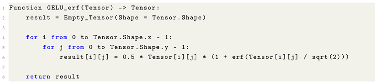 |
As with other activation functions, GELU is applied in an element-wise fashion, facilitating efficient parallelization.
11.8.4. Advantages and Use Cases
GELU (erf-based) provides several critical advantages:
- Smooth Non-linearity: Balances the sparsity introduced by ReLU with the smoothness of sigmoid-like activations.
- Superior Performance in Deep Networks: Empirically shown to improve training stability and accuracy, particularly in Transformer-based architectures.
- Stable Gradient Flow: The smooth, differentiable structure ensures robust gradient propagation even across very deep layers.
- Model Expressiveness: Enables the capture of subtle relationships in high-dimensional data spaces.
- High Performance-to-Complexity Ratio: Especially effective in scaling models to billions of parameters (e.g., BERT, GPT architectures).
11.8.5. Limitations and Practical Considerations
Despite its advantages, GELU (erf-based) introduces specific computational tradeoffs:
- Increased Computational Complexity: Evaluation of the error function is significantly more expensive than basic ReLU or even Swish activations.
- Hardware Efficiency: Less suited for deployment on edge devices or real-time applications due to the higher evaluation cost.
- Potential Overfitting Risk: Due to its ability to closely model complex data patterns, GELU may overfit small or noisy datasets.
- Training Latency: Slower per-epoch training times compared to simpler activations.
- Alternative Approximations: Faster approximations, such as GELU(tanh), are often preferred in production environments to reduce inference time.
11.8.6. Graphical Interpretation of GELU (erf)
As illustrated in Figure 14, the behavior of GELU can be interpreted as:
- Negative Region (): For negative inputs, the output decays smoothly toward zero without abrupt cutoffs. This soft suppression enables minor negative information to contribute to feature learning, while preserving stable gradient flow.
- Positive Region (): For positive inputs, the activation increases approximately linearly, asymptotically approaching the identity line. This behavior maintains strong gradient magnitudes for positive signals, supporting efficient learning.
11.9. Hyperbolic Tangent (tanh): Definition, Properties, and Practical Applications
11.9.1. Intuitive Overview
The hyperbolic tangent (tanh) activation function introduces smooth, zero-centered non-linearity by mapping real-valued inputs into a bounded range between and 1. Conceptually, tanh compresses inputs while preserving their sign and relative magnitude, enabling neural networks to learn balanced representations where both positive and negative activations are meaningful.
11.9.2. Mathematical Definition
Formally, the tanh function is defined as:
where e denotes Euler’s number (). As x approaches positive infinity, ; as x approaches negative infinity, . The function is smooth, continuous, and differentiable everywhere.
11.9.3. Formulaic Pseudocode Implementation
| Listing 27. Formulaic Pythonic Code for tanh Activation. |
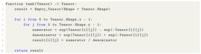 |
As with other activations discussed, tanh operates element-wise, enabling straightforward parallelization in high-dimensional tensor computations.
11.9.4. Advantages and Use Cases
The tanh activation function remains relevant in various Machine Learning applications due to the following properties:
- Zero-centered Output: Unlike sigmoid, tanh outputs are centered around zero, facilitating more balanced gradient updates during optimization.
- Smooth Non-linearity: Provides smooth, continuous gradients conducive to stable learning.
- Use in Recurrent Architectures: Commonly employed in Recurrent Neural Networks (RNNs) where controlling positive and negative signal propagation is beneficial.
- Legacy Neural Architectures: Historically favored in early neural networks for its ability to handle both positive and negative data distributions.
11.9.5. Limitations and Practical Considerations
Despite its advantages, tanh presents certain challenges in deep learning applications:
- Vanishing Gradient Problem: Saturation at extreme input values leads to diminished gradients, impairing learning in deep networks.
- Slower Convergence: Networks using tanh may train slower compared to ReLU-based architectures.
- Limited Suitability for Deep CNNs and Transformers: In modern deep convolutional and Transformer models, activations like ReLU, GELU, or Swish are preferred due to better scaling properties.
- Higher Computational Cost Compared to Piecewise Activations: Requires exponential operations per evaluation.
11.9.6. Graphical Interpretation of tanh
As illustrated in Figure 15, the behavior of tanh can be interpreted as:
- Negative Region (): For negative inputs, smoothly approaches . As inputs become more negative, the function flattens, resulting in smaller gradients and weaker sensitivity to input variations.
- Positive Region (): For positive inputs, increases toward 1 with a similar flattening effect. Near the origin (), tanh behaves approximately linearly, providing strong sensitivity to small changes.
This characteristic “S-shaped” curve enables neural networks to suppress extreme input values while maintaining smooth, interpretable non-linearity, particularly valuable in recurrent learning settings.
11.10. Gaussian Error Linear Unit Approximation (GELU, tanh-based): Definition, Properties, and Practical Applications
11.10.1. Intuitive Overview
The Gaussian Error Linear Unit (GELU) activation function, when approximated using the hyperbolic tangent (tanh) function, provides a computationally efficient variant of the original GELU formulation based on the error function (). The tanh-based approximation introduces smooth non-linearity while maintaining a high-fidelity approximation of the probabilistic gating behavior of GELU, enabling deep networks to model complex patterns effectively with reduced computational overhead.
11.10.2. Mathematical Definition
The tanh-based approximation of GELU is defined as:
Here, the cubic term inside the tanh introduces mild curvature, aligning the approximation closely to the exact GELU curve while significantly accelerating computation.
11.10.3. Formulaic Pseudocode Implementation
| Listing 28. Formulaic Pythonic Code for GELU (tanh) Approximation. |
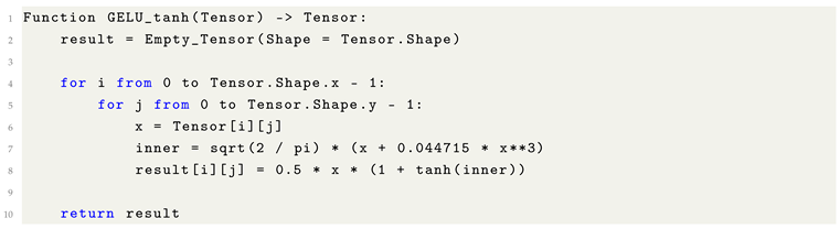 |
As with all activation functions discussed, GELU(tanh) is applied element-wise across the tensor.
11.10.4. Advantages and Use Cases
GELU(tanh) retains many of the core advantages of GELU while offering additional practical benefits:
- Smooth Non-linearity: Maintains smooth gradient flow critical for training deep networks.
- Efficient Computation: Significantly faster to evaluate than the -based GELU, making it suitable for large-scale deployments.
- High-Fidelity Approximation: Provides a close match to the probabilistic behavior of the original GELU formulation.
- Transformer Architectures: Frequently employed in Transformer-based models such as BERT and GPT to balance computational cost with model expressivity.
11.10.5. Limitations and Practical Considerations
Despite its efficiency, GELU(tanh) entails certain trade-offs:
- Approximation Error: Although close, GELU(tanh) is still an approximation and may introduce minor deviations from true probabilistic behavior.
- Higher Cost Compared to ReLU: Still computationally heavier than simple piecewise activations like ReLU or Leaky ReLU.
- Potential Overfitting Risk: As with the exact GELU, its fine-grained sensitivity to input variations can lead to overfitting on small or noisy datasets.
11.10.6. Graphical Interpretation of GELU (tanh)
As illustrated in Figure 16, the behavior of GELU(tanh) can be interpreted as:
- Negative Region (): For negative inputs, the output softly decays toward zero without abrupt cutoffs, preserving minor negative activations. This enables richer feature learning compared to ReLU-like activations.
- Positive Region (): For positive inputs, the function behaves almost linearly for large magnitudes, closely tracking the identity function while maintaining smooth differentiability.
The combination of these behaviors contributes to enhanced learning stability, improved optimization dynamics, and superior generalization in deep architectures.
11.11. Softmax Activation: Definition, Properties, and Practical Applications
11.11.1. Intuitive Overview
The Softmax function transforms a vector of arbitrary real-valued scores into a probability distribution over mutually exclusive classes. By applying exponentiation and normalization, Softmax ensures that each output value is non-negative and that the outputs collectively sum to one. This allows raw model outputs (logits) to be interpreted as human-readable confidence scores, making Softmax a crucial component in multi-class classification tasks.
11.11.2. Step-by-Step Breakdown
The Softmax transformation can be broken into the following conceptual stages, applied to each row or vector independently:
- Stabilization (Optional): To avoid numerical overflow during exponentiation, subtract the maximum value from each element in the vector.
- Exponentiation: Apply the exponential function to each stabilized value, emphasizing larger inputs.
- Summation: Compute the sum of all exponentiated values within the vector.
- Normalization: Divide each exponentiated value by the local sum to produce a normalized probability distribution.
11.11.3. Mathematical Definition
Given an input vector , the Softmax function outputs a vector where:
When stabilization is applied, the formula becomes:
which prevents overflow when values are large.
11.11.4. Formulaic Pseudocode Implementation
| Listing 29. Formulaic Pythonic Code for Softmax Activation. |
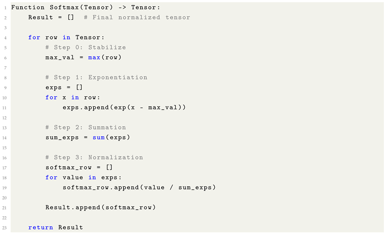 |
Unlike prior element-wise activations (e.g., ReLU, tanh), Softmax is a vector-wise operation—its output for a given element depends on all elements within the same row or vector.
11.11.5. Advantages and Use Cases
Softmax offers several crucial advantages:
- Probabilistic Interpretation: Outputs can be interpreted as class confidence scores.
- Compatibility with Cross-Entropy Loss: When combined with cross-entropy loss, Softmax enables efficient optimization for multi-class classification.
- Human-Readable Outputs: Converts complex logits into easily interpretable probability distributions.
- Multi-Class Decision Making: Facilitates decisions between mutually exclusive outcomes.
11.11.6. Limitations and Practical Considerations
Despite its utility, Softmax is not universally applicable:
- Binary Classification: For binary problems, the sigmoid activation is typically preferred over Softmax.
- Regression Tasks: In regression problems predicting continuous values, Softmax is inappropriate.
- Hidden Layers: Softmax is rarely used in hidden layers, as it constrains activations unnecessarily early in the network.
11.11.7. Application in Multi-Class Output Layers
When a model is tasked with choosing among multiple classes, applying Softmax at the output layer enables probabilistic interpretation:
- Each class receives a probability score between 0 and 1.
- All class scores collectively sum to 1.
- The class with the highest probability is typically selected as the predicted label.
This behavior contrasts with sigmoid activations, which are best suited for independent binary predictions rather than mutually exclusive classification tasks.
11.11.8. Graphical Interpretation of Softmax
As illustrated in Figure 17:
- Each curve corresponds to a different class output.
- As one input becomes dominant, its associated probability sharply rises toward 1, while the probabilities of competing classes decline toward 0.
- The resulting probability vectors remain normalized, ensuring interpretability and consistency.
Conceptually, Softmax generalizes the behavior of the sigmoid function to multi-class settings, offering a smooth and differentiable mapping from real-valued scores to probabilistic decisions.
12. Derivatives of Activation Functions for Backpropagation
In supervised learning with neural networks, the backpropagation algorithm relies fundamentally on the derivatives of activation functions, applying the chain rule of calculus to compute gradients with respect to model parameters. The derivative of an activation function quantifies the sensitivity of a neuron’s output to infinitesimal changes in its input, directly influencing the flow of learning signals during gradient descent optimization.
- Note: In all cases presented, it is assumed that the variable x refers to the input to the activation function during the forward pass, as required by the backpropagation procedure.
12.1. Derivative of the Rectified Linear Unit (ReLU)
The ReLU derivative is defined piecewise. During backpropagation:
- If the pre-activation input , the gradient flows unchanged (multiplied by 1).
- If , the gradient is zeroed out (multiplied by 0).
Formally:
- Formulaic Pseudocode for ReLU Derivative:
| Listing 30. Formulaic Pythonic Code for ReLU Derivative. |
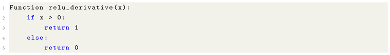 |
The behavior of the ReLU derivative is a major contributor to the “dying ReLU” phenomenon in deep networks, where neurons become permanently inactive.
12.2. Derivative of the Leaky ReLU
The Leaky ReLU derivative modifies the ReLU behavior by allowing a small, non-zero gradient when , controlled by a hyperparameter (e.g., ). During backpropagation:
- If , the derivative is 1.
- If , the derivative is .
Formally:
- Formulaic Pseudocode for Leaky ReLU Derivative:
| Listing 31. Formulaic Pythonic Code for Leaky ReLU Derivative. |
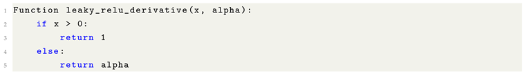 |
By preserving a small gradient for negative inputs, Leaky ReLU mitigates the vanishing gradient issues associated with standard ReLU, improving the robustness of learning dynamics, particularly in very deep or unbalanced networks.
12.3. Derivatives of Advanced Activation Functions
For effective training via backpropagation, the derivatives of activation functions are crucial. They govern the flow of gradients across layers and directly influence optimization dynamics. Below, we formalize the derivatives of Swish, Sigmoid, GELU (erf), and tanh activations.
- Note: All derivatives assume x refers to the input to the activation function unless otherwise specified.
12.3.1. Derivative of Swish Activation
The Swish activation, defined as , has a derivative:
where is the sigmoid function.
- Formulaic Pseudocode for Swish Derivative:
| Listing 32. Formulaic Pythonic Code for Swish Derivative. |
 |
Alternatively, if only computing is desired for efficiency:
| Listing 33. Sigmoid Helper Function for Swish Derivative. |
 |
12.3.2. Derivative of Sigmoid Activation
The derivative of the Sigmoid activation, , is:
where denotes the sigmoid output.
- Formulaic Pseudocode for Sigmoid Derivative:
| Listing 34. Formulaic Pythonic Code for Sigmoid Derivative. |
 |
This compact form allows reusing the forward-pass sigmoid result during backpropagation, improving computational efficiency.
12.3.3. Derivative of GELU (erf-based)
The GELU activation, defined via the Gaussian error function, has a derivative:
where is the error function.
- Formulaic Pseudocode for GELU (erf) Derivative:
| Listing 35. Formulaic Pythonic Code for GELU (erf) Derivative. |
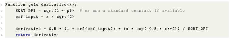 |
The derivative captures both the smoothness and the probabilistic gating effect inherent in GELU activations.
12.3.4. Derivative of tanh Activation
The derivative of the hyperbolic tangent activation, , is:
where is the forward activation output.
- Formulaic Pseudocode for tanh Derivative:
| Listing 36. Formulaic Pythonic Code for tanh Derivative. |
 |
This structure, similar to the sigmoid derivative, facilitates efficient computation during backpropagation by leveraging cached forward-pass outputs.
12.4. Derivative of GELU (tanh-based Approximation)
The tanh-based approximation of the Gaussian Error Linear Unit (GELU) is computationally efficient and widely used in Transformer-based architectures. Given the approximation:
its derivative with respect to x is:
This derivative smoothly modulates gradient flow and is more computationally tractable than the exact -based form.
- Formulaic Pseudocode for GELU(tanh) Derivative:
| Listing 37. Formulaic Pythonic Code for GELU (tanh) Derivative. |
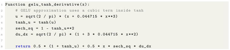 |
This form ensures compatibility with auto-differentiation frameworks and provides smooth, stable gradients during backpropagation.
12.5. Derivative of Softmax (and Its Practical Simplification)
The Softmax function is defined as:
Its derivative is formally given by the Jacobian matrix:
This results in a dense Jacobian matrix that is seldom computed directly in practice.
- Practical Note: In modern machine learning pipelines, Softmax is almost exclusively paired with cross-entropy loss. The gradient of their composition simplifies considerably:
Therefore, while the theoretical derivative of Softmax is well-defined, it is typically bypassed via this simplification in the context of supervised learning.
13. Loss Functions: Formal Definitions and Computational Structure
In supervised learning, loss functions quantify the divergence between a model’s predictions and the true target outputs. During training, the optimization algorithm—typically a gradient-based method—uses these loss values to iteratively adjust the model’s parameters with the goal of minimizing prediction error.
Loss is not to be confused with error itself. While error often refers to the raw difference between predicted and actual values, loss functions translate that discrepancy into a single scalar quantity optimized during learning.
- Note: Unless otherwise specified, all functions assume that input tensors are of equal shape and appropriately batched.
13.1. Mean Absolute Error (MAE)
MAE computes the mean of the absolute differences between predicted and actual values:
- Formulaic Pseudocode for MAE:
| Listing 38. Formulaic Pythonic Code for Mean Absolute Error (MAE). |
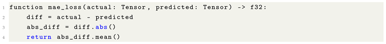 |
13.2. Mean Squared Error (MSE)
MSE penalizes larger deviations more strongly than MAE by squaring the errors:
- Formulaic Pseudocode for MSE:
| Listing 39. Formulaic Pythonic Code for Mean Squared Error (MSE). |
 |
13.3. Hinge Loss
Hinge loss is used primarily for binary classification with Support Vector Machines (SVMs). It encourages a decision boundary with a margin:
- Formulaic Pseudocode for Hinge Loss:
| Listing 40. Formulaic Pythonic Code for Hinge Loss. |
 |
13.4. Huber Loss
Huber loss combines the advantages of MAE and MSE. For small errors, it behaves quadratically (like MSE), while for large errors, it behaves linearly (like MAE), thus improving robustness to outliers:
- Formulaic Pseudocode for Huber Loss:
| Listing 41. Formulaic Pythonic Code for Huber Loss. |
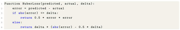 |
13.5. Binary Cross-Entropy (BCE)
BCE is commonly used in binary classification. It quantifies the divergence between predicted probabilities and actual binary labels:
To avoid logarithmic instability, predictions are typically clamped using a small constant .
- Formulaic Pseudocode for BCE:
| Listing 42. Formulaic Pythonic Code for Binary Cross-Entropy (BCE). |
 |
13.6. Categorical Cross-Entropy (CCE)
CCE generalizes BCE to multi-class settings. It penalizes incorrect class probabilities based on a one-hot encoded label:
- Formulaic Pseudocode for CCE:
| Listing 43. Formulaic Pythonic Code for Categorical Cross-Entropy (CCE). |
 |
Table 4.
Summary of Common Loss Functions and Their Behavior
| Loss Function | Key Behavior |
|---|---|
| Mean Absolute Error (MAE) | Treats all errors equally by measuring the absolute difference between actual and predicted values. |
| Mean Squared Error (MSE) | Penalizes larger errors more severely by squaring them, making the model more sensitive to outliers. |
| Hinge Loss | Builds a margin of safety around classes, encouraging confident classification boundaries (commonly used in Support Vector Machines). |
| Huber Loss | Smoothly combines MAE and MSE behavior: acts like MSE for small errors and MAE for large errors, making it robust to outliers. |
| Binary Cross Entropy (BCE) | Measures the difference between two probability distributions in binary classification tasks (two classes: 0 or 1). |
| Categorical Cross Entropy (CCE) | Extends Cross Entropy to multi-class classification problems, comparing predicted probability distributions over multiple categories. |
14. Optimizers: Theory and Role in Training Dynamics
In machine learning, particularly in gradient-based neural network training, an optimizer is an algorithm that governs how a model’s parameters are updated during learning. At the core of this process lies the concept of the learning rate—a hyperparameter that controls the size of the updates applied to model weights in response to the loss gradient.
Optimizers aim to minimize the loss function by iteratively adjusting the model’s parameters in the direction of steepest descent (or approximations thereof). While basic methods apply a fixed learning rate and simple updates, more advanced optimizers adaptively modify the learning rate over time, incorporate past gradients, and regularize the updates to improve convergence speed and stability.
The choice of optimizer plays a critical role in determining:
- The speed of convergence toward a solution.
- The stability of training across varying data distributions.
- The model’s ability to escape local minima or saddle points.
- Generalization performance on unseen data.
This section presents both classical and modern optimization algorithms, each accompanied by its update rule, key characteristics, and usage considerations.
Table 5.
Comparison of Adam and SGD Optimizers
| Aspect | Adam Optimizer | SGD Optimizer |
|---|---|---|
| Learning Rate Adjustment | Adaptive learning rate for each parameter | Fixed or manually decayed learning rate |
| Speed of Convergence | Faster convergence, especially early on | Slower convergence without momentum |
| Memory Usage | Higher (stores moment estimates) | Lower (only stores gradients) |
| Sensitivity to Learning Rate | Less sensitive to initial learning rate choice | Highly sensitive to learning rate choice |
| Use Case | Good for complex networks, sparse gradients | Good for simple or very large datasets |
| Mathematical Complexity | More complex (uses moving averages of gradients) | Simpler (straightforward gradient update) |
Traditional optimizers such as Stochastic Gradient Descent (SGD) update parameters by stepping proportionally to the negative gradient. However, more sophisticated optimizers like Adam introduce adaptive learning rates and momentum, greatly improving convergence speed and stability.
14.1. Adam Optimizer (Adaptive Moment Estimation)
The Adam optimizer is a first-order gradient-based optimization algorithm that adaptively adjusts the learning rate for each parameter based on estimates of the first and second moments of the gradients. Introduced by Kingma and Ba (2015), Adam merges the benefits of Momentum (smoothing using first moments) and RMSProp (normalization using second moments) into a single, robust method.
Formally, Adam maintains two exponentially decaying averages:
- – the exponentially weighted moving average of past gradients (first moment estimate)
- – the exponentially weighted moving average of squared gradients (second moment estimate)
To correct bias introduced during initialization, bias-corrected estimates are computed:
The parameter update rule becomes:
where:
- – current parameter value
- – learning rate (default: )
- – small constant for numerical stability (e.g., )
- – decay rates for the first and second moment estimates (typically , )
- Formulaic Pythonic Pseudocode for Adam Optimizer:
| Listing 44. Formulaic Pythonic Code for Adam Optimizer. |
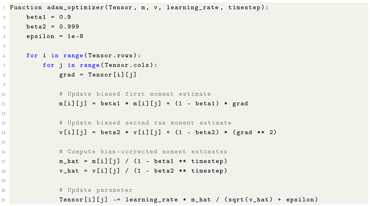 |
Advantages of Adam
- Adaptive learning rate per parameter
- Requires minimal tuning and is robust to sparse gradients
- Combines fast convergence with stability in non-stationary settings
- Well-suited for large models and noisy objective functions
Limitations and Practical Notes
- Adam may sometimes lead to overfitting or poor generalization compared to SGD with momentum in certain vision tasks.
- Learning rate warm-up, weight decay (AdamW), or switching to SGD mid-training are often employed for better results.
- Commentary: While basic stochastic gradient descent (SGD) is inherently integrated into the backpropagation update rule, optimizers like Adam offer substantial performance gains in training time and convergence speed—particularly in deep and high-dimensional architectures.
14.2. Stochastic Gradient Descent (SGD)
Stochastic Gradient Descent (SGD) is the most fundamental optimization algorithm in machine learning and serves as the theoretical basis for more advanced methods. SGD seeks to minimize a loss function by iteratively updating model parameters in the direction of the negative gradient.
Unlike full-batch gradient descent, which computes gradients over the entire training dataset at each step, SGD performs updates using a single sample (or mini-batch), defined as:
where:
- – learning rate
- – the training example or mini-batch
- – gradient of the loss with respect to model parameters
By introducing stochasticity through random sampling, SGD helps models escape shallow local minima and saddle points, particularly in high-dimensional, non-convex optimization landscapes.
- Formulaic Pseudocode for SGD:
| Listing 45. Formulaic Pythonic Code for SGD Optimizer. |
 |
Advantages of SGD
- Simple to implement and computationally efficient.
- Well-suited for very large datasets (via mini-batch training).
- Can generalize well when combined with regularization and proper learning rate scheduling.
Limitations and Practical Notes
- Convergence may be slow and noisy without momentum or learning rate decay.
- Requires careful tuning of the learning rate to avoid divergence or stagnation.
- Prone to getting stuck in sharp local minima or saddle points in complex loss surfaces.
- Note: SGD is essentially a direct implementation of the backpropagation update rule and is thus already integrated into the core mechanics of neural network training. Its simplicity makes it a standard benchmark and starting point for optimizer comparisons.
15. Normalization: Mitigating Gradient Instabilities in Deep Learning
One of the primary challenges in training deep neural networks is the instability of gradients—specifically, the phenomena of vanishing gradients and exploding gradients. These arise when the magnitude of gradients becomes excessively small or large, causing either stalled learning or numerical overflow, particularly in networks with many layers or poorly scaled inputs.
Normalization techniques are designed to mitigate these issues by rescaling data into numerically manageable ranges. This preserves essential distributional characteristics while reducing the risk of pathological gradients during backpropagation.
Two of the most common normalization strategies are:
- Min-Max Normalization rescales input features to a predefined range, usually , preserving relative proportions.
- Z-Score Standardization (Standard Scaling) centers the data around zero and scales it to unit variance, promoting symmetry in gradient flow.
- Comparison of Normalization Methods:
Table 6.
Comparison of Min-Max Normalization and Z-Score Standardization
| Feature | Min-Max Normalization | Z-Score Standardization |
|---|---|---|
| Range after scaling | Typically ; customizable bounds | Centered around 0 with unit variance |
| Sensitive to outliers? | Highly sensitive | More robust due to variance scaling |
| Use case examples | Pixel intensities, bounded sensors | ML models assuming Gaussian features |
| Effect on distribution | Linear rescaling; preserves original shape | Normalizes spread and location |
| When to use? | When known min/max bounds exist | When data is approximately normal |
- Practical Note: Normalization is not strictly required for all models, but it plays a pivotal role in stabilizing gradient-based training processes. For networks prone to exploding/vanishing gradients, appropriate normalization can dramatically improve convergence rates and model robustness.
15.1. Z-Score Normalization (Standardization)
Z-score normalization, also referred to as standardization, transforms data such that the resulting distribution has zero mean and unit variance. This technique is particularly effective when the underlying data distribution is approximately Gaussian.
Given a tensor X with elements , the standardized form is:
- Formulaic Pythonic Pseudocode for Standardization:
| Listing 46. Formulaic Pythonic Code for Z-Score Normalization. |
 |
Use Cases
- Effective when model assumptions include normally distributed features.
- Common in linear regression, logistic regression, SVMs, and neural networks.
15.2. Min-Max Normalization
Min-Max normalization rescales each element in the dataset to a fixed range, typically , by subtracting the minimum and dividing by the range. It preserves the shape of the original distribution and is highly interpretable but sensitive to outliers.
The transformation is defined as:
- Formulaic Pythonic Pseudocode for Min-Max Normalization:
| Listing 47. Formulaic Pythonic Code for Min-Max Normalization. |
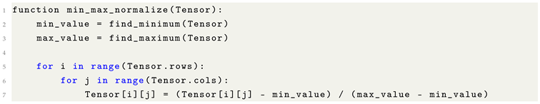 |
Use Cases
- Image pixel scaling (e.g., from to ).
- Features with known and bounded value ranges.
- Practical Note: Min-max normalization assumes a stable range. In the presence of outliers or shifting distributions (e.g., in online learning), Z-score standardization or robust scaling may be preferred.
16. Tensor/Weights and Biases Initialization
Proper initialization of weights and biases plays a pivotal role in stabilizing training dynamics and promoting efficient convergence in deep learning models. In particular, poor initialization can cause gradients to vanish or explode as they are propagated through layers—issues that severely hinder or prevent learning.
To address this, various initialization schemes have been developed to align the variance of activations and gradients across layers, depending on the choice of activation function and model architecture.
- General Principles of Initialization
- Variance Preservation: Maintaining activation variance across layers prevents gradient shrinkage or amplification.
- Activation Function Dependency: Initialization should match the non-linearity used (e.g., ReLU vs. tanh).
- Symmetry Breaking: All weights must be initialized independently to allow neurons to learn distinct features. Biases may be initialized to zero.
The following table summarizes widely adopted initialization strategies:
Table 7.
Summary of Common Weight Initialization Methods and Their Core Characteristics
| Initialization Method | Key Characteristics and Use Cases |
|---|---|
| Xavier (Glorot) |
|
| He (Kaiming) |
|
| Zero Initialization |
|
| Random Uniform |
|
- Practical Note
Weight initialization should always be selected in tandem with the activation function and network architecture. For deep networks using ReLU or GELU activations, He initialization is typically preferred. For sigmoid or tanh-based networks, Xavier initialization is more appropriate.
Biases, unless specifically tuned (e.g., for LSTMs or BatchNorm), are typically initialized to zero.
16.1. Zero Initialization
Zero initialization sets all weights in a neural network layer to zero. While this method is computationally efficient and trivial to implement, it introduces a fundamental flaw: all neurons in a given layer receive identical gradients during backpropagation and thus learn the same features. This symmetry prevents the network from effectively breaking degeneracy in weight space.
Key Drawbacks:
- Fails to break symmetry between neurons.
- Leads to vanishing gradients and stalled learning.
- Only suitable for initializing biases.
16.2. Pseudo-Random Initialization (Uniform)
Random uniform initialization generates weights using a uniform distribution within a specified range (e.g., ). While it avoids the symmetry problem seen in zero initialization, it does not scale based on network depth or activation function, and thus may lead to unstable training in deep architectures.
Formulaic Pythonic Pseudocode:
| Listing 48. Random Uniform Tensor Initialization. |
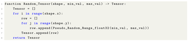 |
- Note: For uniform initialization, a common range is . This should be adjusted depending on layer size and depth.
16.3. Xavier (Glorot) Initialization
Xavier (or Glorot) initialization is designed to preserve the variance of activations across layers when using tanh or sigmoid activations. It draws weights from a uniform distribution with bounds based on the number of input and output units.
Formulaic Pythonic Pseudocode:
| Listing 49. Formulaic Pythonic Code for Xavier Initialization. |
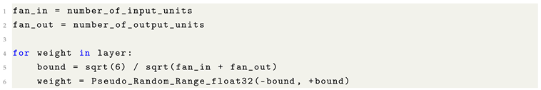 |
Best suited for: Activation functions such as sigmoid, tanh
16.4. He Initialization
He initialization (also called Kaiming initialization) is tailored for layers using ReLU or Leaky ReLU activations. It initializes weights by sampling from a normal distribution with zero mean and a standard deviation of:
Formulaic Pythonic Pseudocode:
| Listing 50. Formulaic Pythonic Code for He Initialization. |
 |
Best suited for: ReLU, Leaky ReLU, ELU, GELU
Advantages:
- Helps avoid vanishing gradients.
- Promotes stable signal propagation in deep networks.
- Generally converges faster in deep architectures with ReLU-based activations.
17. Backpropagation: The Core Learning Algorithm in Neural Networks
Backpropagation is the central algorithm responsible for training neural networks via supervised learning. It refines a model’s internal parameters—namely, weights and biases—by propagating the error signal backward through the network, layer by layer, and computing gradients that guide each parameter update.
This process is built upon the chain rule of calculus, which allows the computation of how the loss changes with respect to every parameter in the network, even deep within multiple layers. When paired with gradient-based optimization algorithms such as Stochastic Gradient Descent (SGD) or Adam, backpropagation enables neural networks to approximate complex, nonlinear functions from data.
The training process typically consists of four key stages:
- Forward Pass – Computes activations layer by layer using current weights and biases.
- Loss Function Evaluation – Measures the discrepancy between the model’s prediction and the true target.
- Backward Pass – Propagates the loss gradient backward through the network, computing parameter-wise gradients.
- Gradient Descent Step – Updates weights and biases using gradients and a selected optimization algorithm.
17.1. Key Computational Tools for Backpropagation
To implement backpropagation from first principles, the following computational primitives are essential:
- Matrix Multiplication – Enables dot products between weights and activations.
- Transposition – Required for aligning gradients across layer interfaces.
- Element-wise Operations – Applied to activation outputs and error signals.
- Activation Functions and Their Derivatives – Nonlinearities such as ReLU, tanh, or sigmoid must support differentiation.
17.2. Forward Pass
The forward pass processes inputs sequentially through the network’s layers. Each layer computes:
Where:
- is the pre-activation output of layer l,
- and are the weight matrix and bias vector,
- is the activation function (e.g., ReLU, tanh),
- is the post-activation output, passed to the next layer.
This process continues through all hidden layers and concludes at the output layer.
17.3. Loss Function
The loss function quantifies prediction error. Common examples include:
The choice of loss function depends on the task (e.g., regression vs. classification) and impacts gradient computation.
17.4. Backward Pass (Backpropagation)
The backward pass computes the gradient of the loss function with respect to each weight and bias in the network by traversing layers in reverse. This relies on repeated application of the chain rule:
-
Steps:
- Compute error gradient at the output layer.
- Propagate this error backwards through hidden layers.
- Multiply by activation function derivative.
- Use the gradients to update parameters.
- Formulaic Pythonic Pseudocode:
| Listing 51. Formulaic Pythonic Code for Backpropagation. |
 |
Figure 18.
Breakdown of the backward pass in formulaic pseudocode.
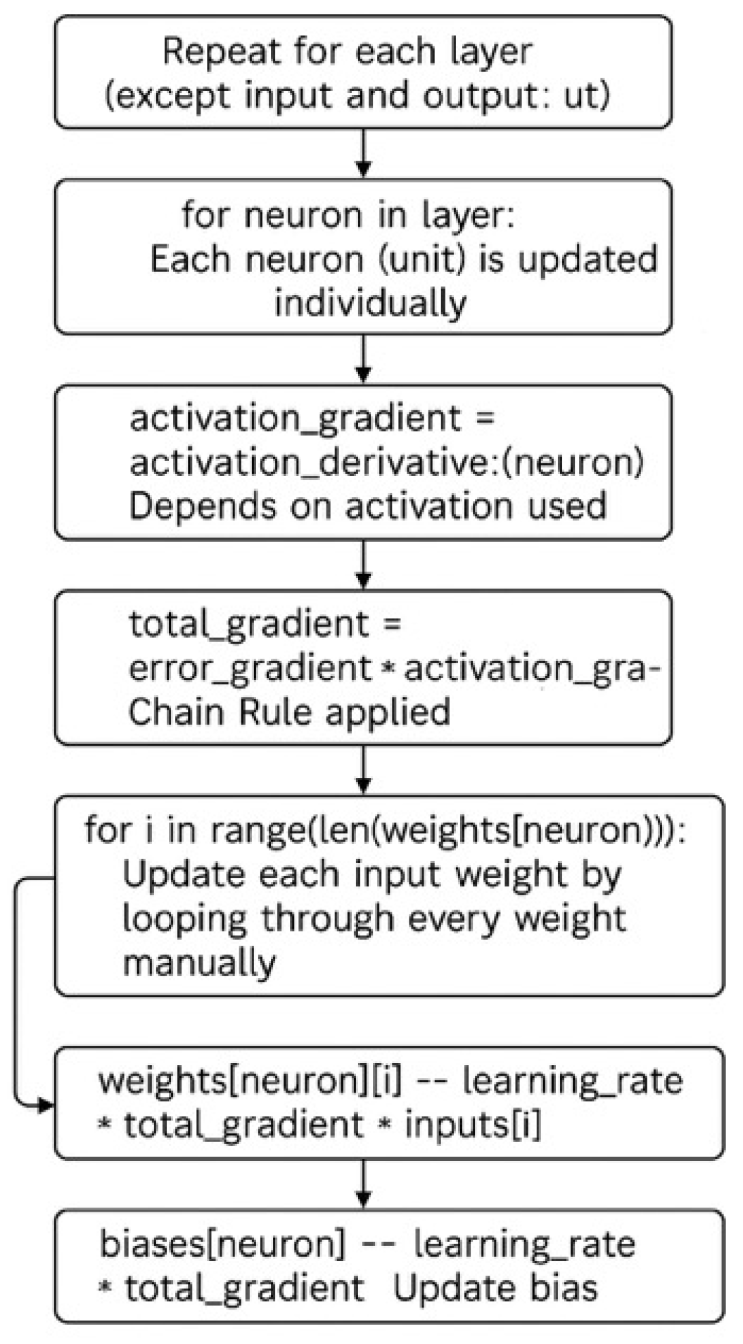
17.5. Gradient Descent Step
Once gradients are computed, they are used to update model parameters:
This step may be implemented using SGD or more sophisticated optimizers (e.g., Adam, RMSProp) discussed earlier.
17.6. Batch Training and Epochs
Training is typically performed in mini-batches for computational efficiency and generalization. A full dataset pass is called an epoch. The backpropagation cycle is repeated across batches and epochs to progressively reduce the loss.
17.7. Summary: The Backpropagation Pipeline
Backpropagation is the engine that drives learning in neural networks. It enables the network to systematically refine its parameters to minimize a loss function, translating gradient signals into corrective updates. The algorithm’s structure, forward pass, loss computation, backward pass, and parameter update, forms the training loop at the heart of nearly all modern deep learning architectures.
Mastering backpropagation offers both a practical and theoretical foundation for understanding how complex models generalize, optimize, and ultimately learn to represent abstract patterns in data.
Recent Advances
In recent years, substantial progress has been made in machine learning techniques, optimization methods, and model architectures. Innovations such as the Adam optimizer [1] and its improved variant AdamW [2] have reshaped training dynamics. Transformer architectures [3] introduced self-attention mechanisms that are now foundational across domains. Improvements in activation functions, including GELU [4] and Swish [5], have enhanced non-linearity handling. Regularization strategies like Cutout [6], Mixup [7], and RICAP [8] have strengthened model robustness.
New approaches to optimization such as RAdam [9], Lookahead [10], and AdaBelief [11] have emerged, refining convergence stability. Advances in normalization techniques like LayerNorm [12], GroupNorm [13], and EvoNorm [14] have further improved the training of deep models. Weight initialization strategies like He initialization [15] and Fixup initialization [16] addressed challenges in very deep networks.
Recent network architectures, such as EfficientNet [17], ResNeSt [18], and ConvNeXt [19], have pushed the frontier of computer vision benchmarks. Self-supervised learning techniques like SimCLR [20] and BYOL [21] have unlocked new paradigms for representation learning without extensive labels.
These developments reflect an active and rapidly evolving field, providing a strong foundation for further innovation and accessibility in machine learning education.
18. Conclusion
This work has aimed to demystify and recontextualize the mathematical foundations of Machine Learning (ML) in order to reduce the barriers that often exclude highly capable developers, particularly those without formal training in calculus or theoretical mathematics. By translating core ML concepts into formulaic pseudocode and structured algorithmic logic, we advocate for a more inclusive framework, one that recognizes programming expertise as an equally valid and powerful entry point into the field.
Many developers today possess extensive knowledge in low-level systems engineering, embedded computing, Linux kernel development, and WebAssembly. These skillsets are often disconnected from ML discourse due to the pervasive assumption that mastery in advanced calculus is a prerequisite for meaningful participation. This dual requirement, proficiency in both abstract mathematics and complex coding, creates what may be termed the double-genius barrier, which inhibits broader innovation.
By reducing this barrier through pedagogical reform and accessible explanations, we can accelerate cross-disciplinary collaboration and invite contributions from a much wider talent pool. In doing so, the Machine Learning community stands to benefit from a more diverse, global influx of ideas, tools, and methodologies.
18.1. Guidelines for Increasing Accessibility in Machine Learning Education
To support this vision, the following principles are proposed:
- Avoid exclusive reliance on calculus-based notation. While mathematically rigorous exposition remains vital for theoretical development, educational materials should accompany such expressions with structured pseudocode or executable logic wherever possible.
- Recognize programming fluency as foundational. ML is ultimately implemented through code. Prioritizing algorithmic clarity ensures that practitioners from software engineering and systems programming domains can meaningfully engage with and apply ML principles.
- Promote hybrid explanations. Ideal instructional content should bridge formal mathematics and operational intuition—using diagrams, modular code, and relatable metaphors.
Such approaches will empower self-taught programmers, bootcamp graduates, and systems engineers alike, unlocking contributions from communities historically sidelined by overly theoretical teaching methods.
18.2. Machine Learning Without Walls: A Vision for Global Innovation
Imagine a future in which:
- Mathematicians focus exclusively on developing faster and more biologically realistic activation functions, such as novel generalizations of the Hodgkin–Huxley model.
- Systems engineers embed neural inference directly into operating system kernels to achieve ultra-low-latency pattern recognition.
- Educators adopt accessible frameworks for teaching ML logic, allowing students to implement and experiment before ever seeing formal integrals.
Such a future is only possible if we stop requiring every contributor to split their energy equally between two orthogonal skill sets. Let mathematicians build better theory. Let programmers build faster, safer systems. Let educators build bridges between them. In combination, not in isolation, these communities can accelerate the future of Machine Learning far beyond what any single discipline could accomplish alone.
To the mathematicians: You do not have to carry the future of Machine Learning alone. To the programmers: Your intuition, structure, and systems thinking are just as vital. Together, we can dismantle the barriers that no one discipline can overcome in isolation.
To mathematicians: you don’t have to carry the future of Machine Learning alone. To programmers: your skills are just as vital. Together, we can break barriers that no single discipline could ever overcome.
18.3. A Complete Machine Learning Network Example
To demonstrate how the foundational principles discussed in this paper can be applied in practice, Figure 19 presents a complete example of a machine learning pipeline. This network is intentionally designed with transparency and educational clarity, enabling learners to follow each computational step.
| Listing 52. Formulaic Pythonic Code for Example Complete machine learning network flow. |
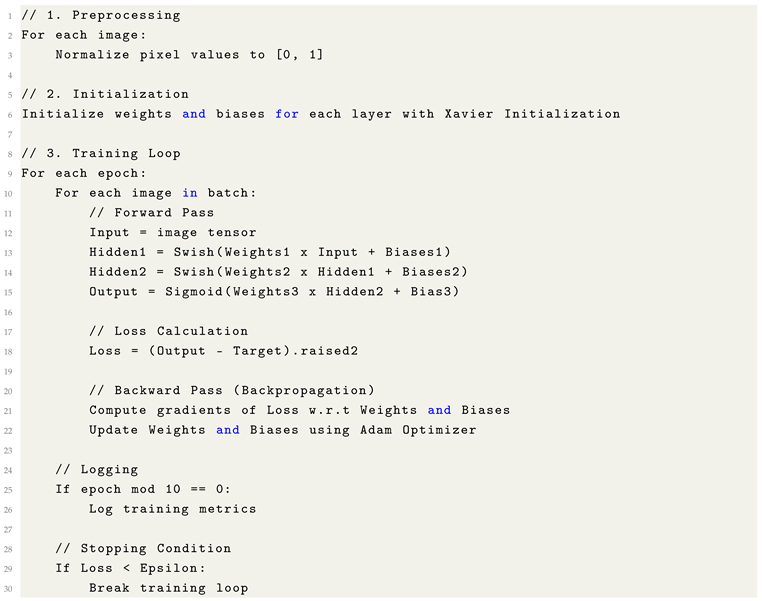 |
19. Final Reflection: The Power of Formulaic Thinking
To conclude, this example shows that the entire machine learning process can be captured cleanly through formulaic pseudocode, without hiding behind walls of pure math. From image preprocessing to network layer transitions, activations, optimization, and backpropagation, every step remains clear and accessible.
While mathematical notation like:
is powerful, it often skips the operational thinking that real-world engineering demands.
Formulaic pseudocode, however, preserves the logic path step-by-step, making it easier to bridge understanding between mathematics and practical implementation.
This bridge is crucial.
By empowering both mathematicians and programmers to see through each other’s worlds more clearly, we can push forward a future where neural networks are not only more powerful but also more understandable and accessible to all learners.
References
- Kingma, D.P.; Ba, J. Adam: A Method for Stochastic Optimization; ICLR, 2015. [Google Scholar]
- Loshchilov, I.; Hutter, F. Decoupled Weight Decay Regularization; ICLR, 2019. [Google Scholar]
- Vaswani, A.; et al. Attention Is All You Need; NeurIPS, 2017. [Google Scholar]
- Hendrycks, D.; Gimpel, K. Gaussian Error Linear Units (GELUs). 2016, arXiv:1606.08415. [Google Scholar]
- Ramachandran, P.; et al. Searching for Activation Functions. 2017, arXiv:1710.05941. [Google Scholar]
- De Vries, T.; Taylor, G.W. Improved Regularization of Convolutional Neural Networks with Cutout. 2017, arXiv:1708.04552. [Google Scholar]
- Zhang, H.; et al. mixup: Beyond Empirical Risk Minimization; ICLR, 2018. [Google Scholar]
- Takahashi, R.; Matsubara, T.; Yoshino, K. RICAP: Random Image Cropping and Patching Data Augmentation for Deep CNNs; ACML, 2018. [Google Scholar]
- Liu, L.; et al. On the Variance of the Adaptive Learning Rateand Beyond. 2019, arXiv:1908.03265. [Google Scholar]
- Zhang, M.R.; et al. Lookahead Optimizer: k steps forward, 1 step back; NeurIPS, 2019. [Google Scholar]
- Zhuang, J.; et al. AdaBelief Optimizer: Adapting Stepsizes by the Belief in Observed Gradients; NeurIPS, 2020. [Google Scholar]
- Ba, J.; Kiros, J.R.; Hinton, G. Layer Normalization. 2016, arXiv:1607.06450. [Google Scholar]
- Wu, Y.; He, K. Group Normalization; ECCV, 2018. [Google Scholar]
- Liu, Z.; et al. EvoNorm: Evolutionary Normalization for Deep Learning. 2020, arXiv:2004.02967. [Google Scholar]
- He, K.; et al. Delving Deep into Rectifiers: Surpassing Human-Level Performance; ICCV, 2015. [Google Scholar]
- Zhang, H.; et al. Fixup Initialization: Residual Learning Without Normalization; ICLR, 2019. [Google Scholar]
- Tan, M.; Le, Q.V. EfficientNet: Rethinking Model Scaling; ICML, 2019. [Google Scholar]
- Zhang, H.; et al. ResNeSt: Split-Attention Networks. 2020, arXiv:2004.08955. [Google Scholar]
- Liu, Z.; et al. A ConvNet for the 2020s; CVPR, 2022. [Google Scholar]
- Chen, T.; et al. A Simple Framework for Contrastive Learning; ICML, 2020. [Google Scholar]
- Grill, J.-B.; et al. Bootstrap Your Own Latent (BYOL); NeurIPS, 2020. [Google Scholar]
Figure 11.
Visualization of Leaky ReLU Activation Function.
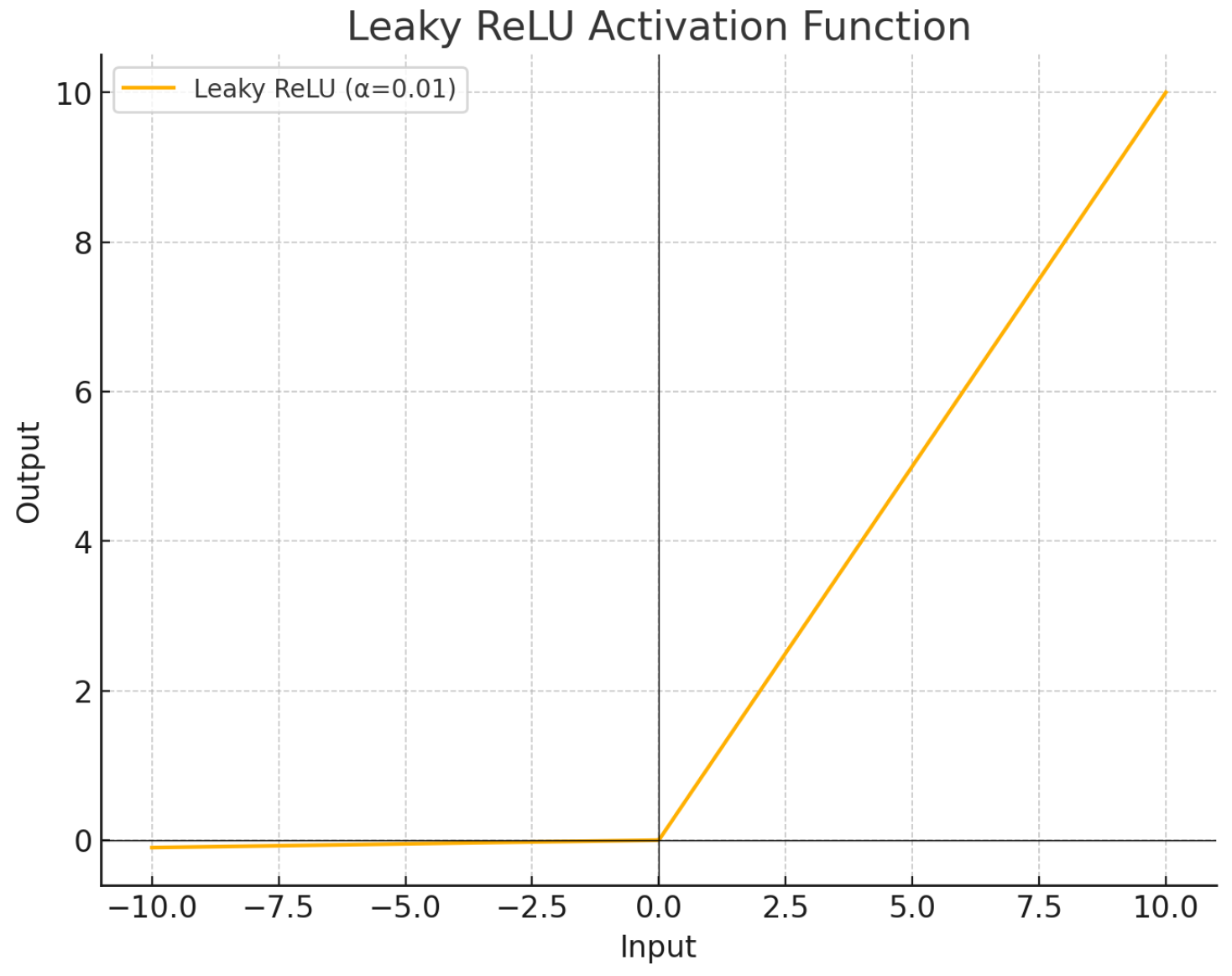
Figure 12.
Graph of the Swish activation function illustrating its behavior across input domains.
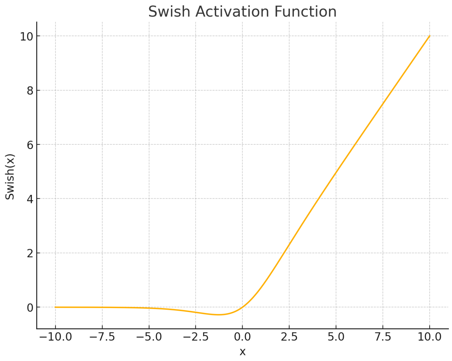
Figure 13.
Graph of the Sigmoid activation function. Although it visually appears to saturate at 0 and 1, these values are approached asymptotically but never exactly attained.
Figure 13.
Graph of the Sigmoid activation function. Although it visually appears to saturate at 0 and 1, these values are approached asymptotically but never exactly attained.
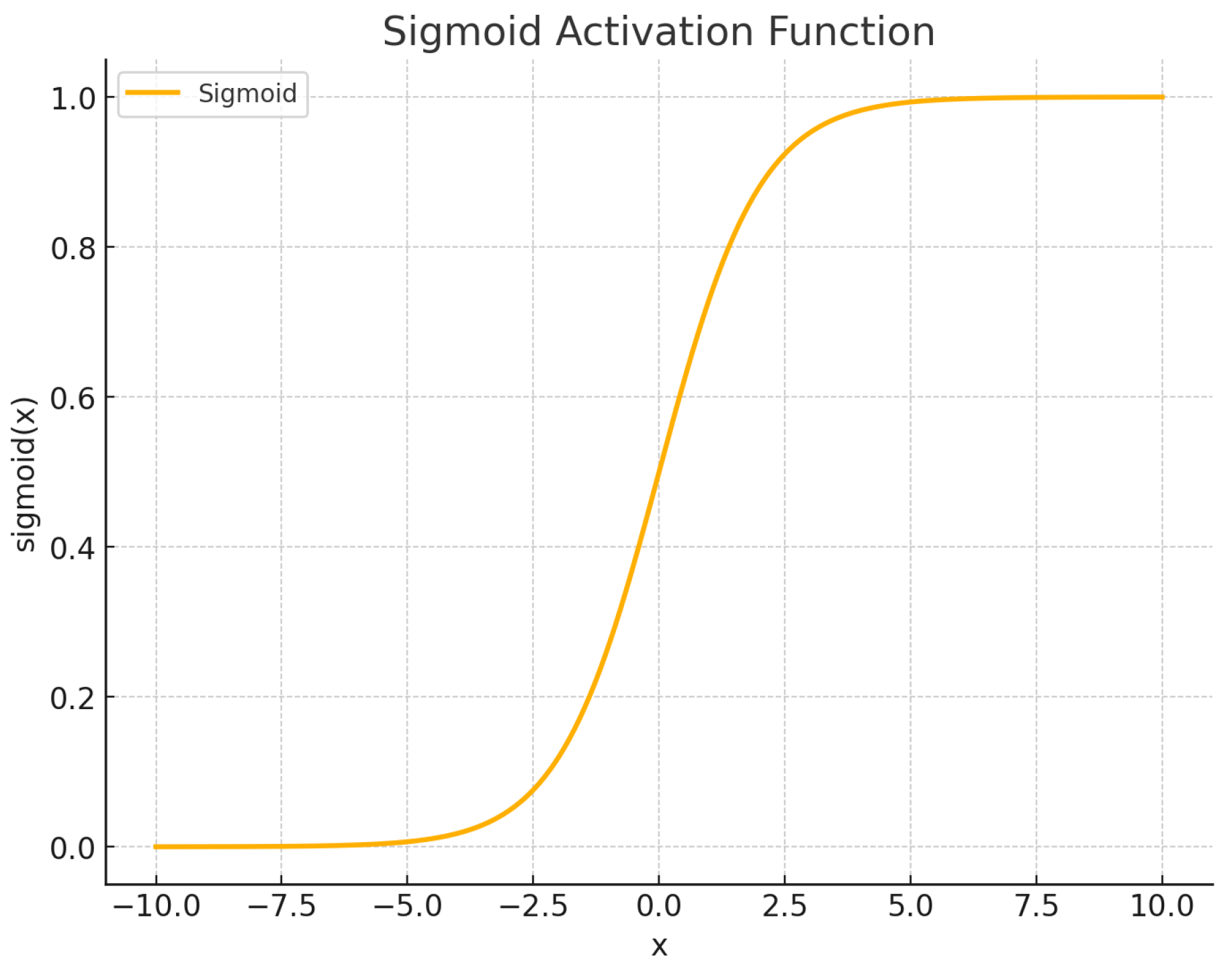
Figure 14.
Graph of the GELU (erf-based) activation function, illustrating its smooth gating behavior across input domains.
Figure 14.
Graph of the GELU (erf-based) activation function, illustrating its smooth gating behavior across input domains.
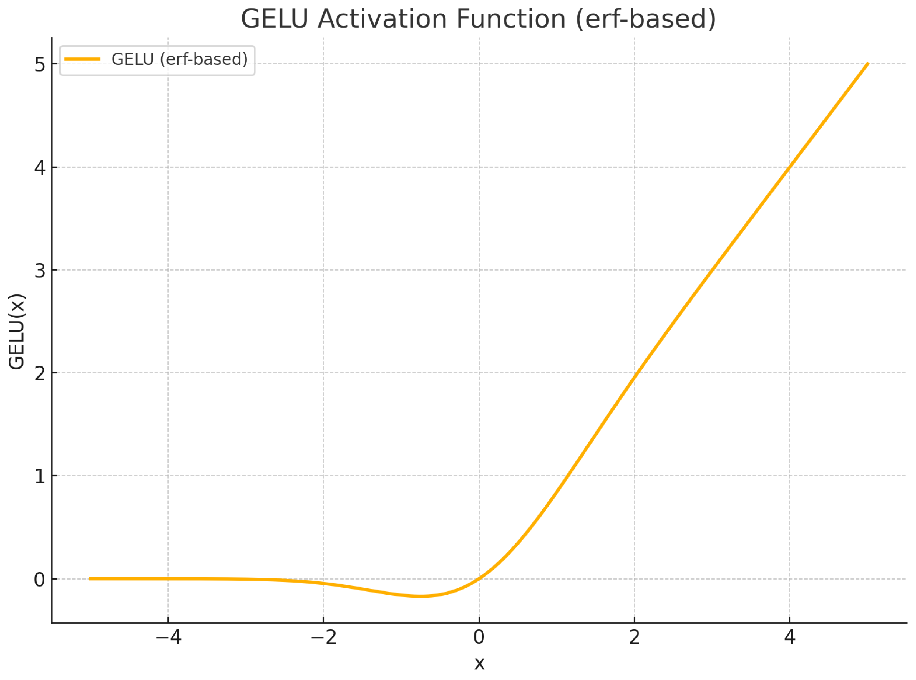
Figure 15.
Graph of the tanh activation function, illustrating its smooth transition from to 1.
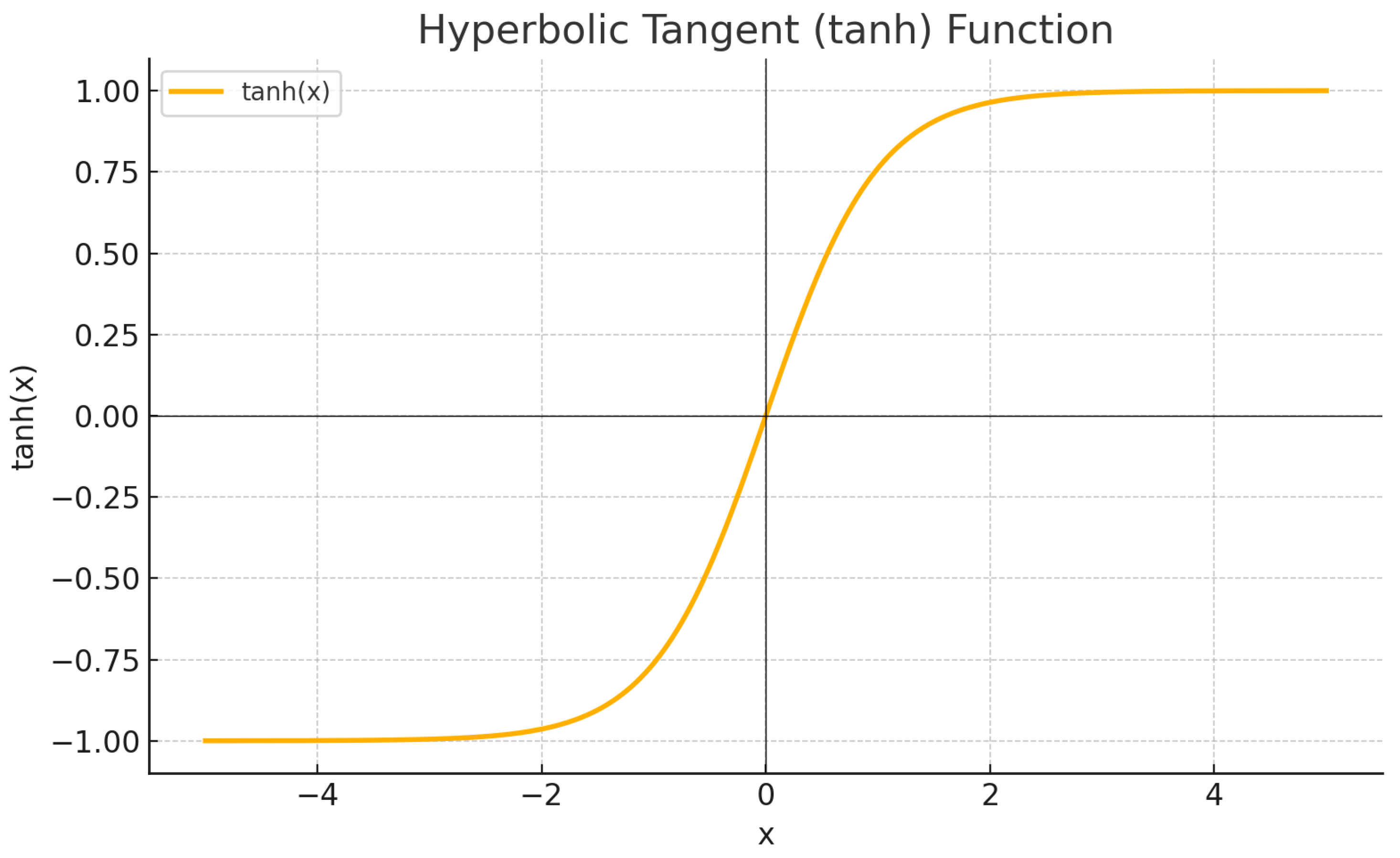
Figure 16.
Graph of the GELU activation function using the tanh-based approximation.
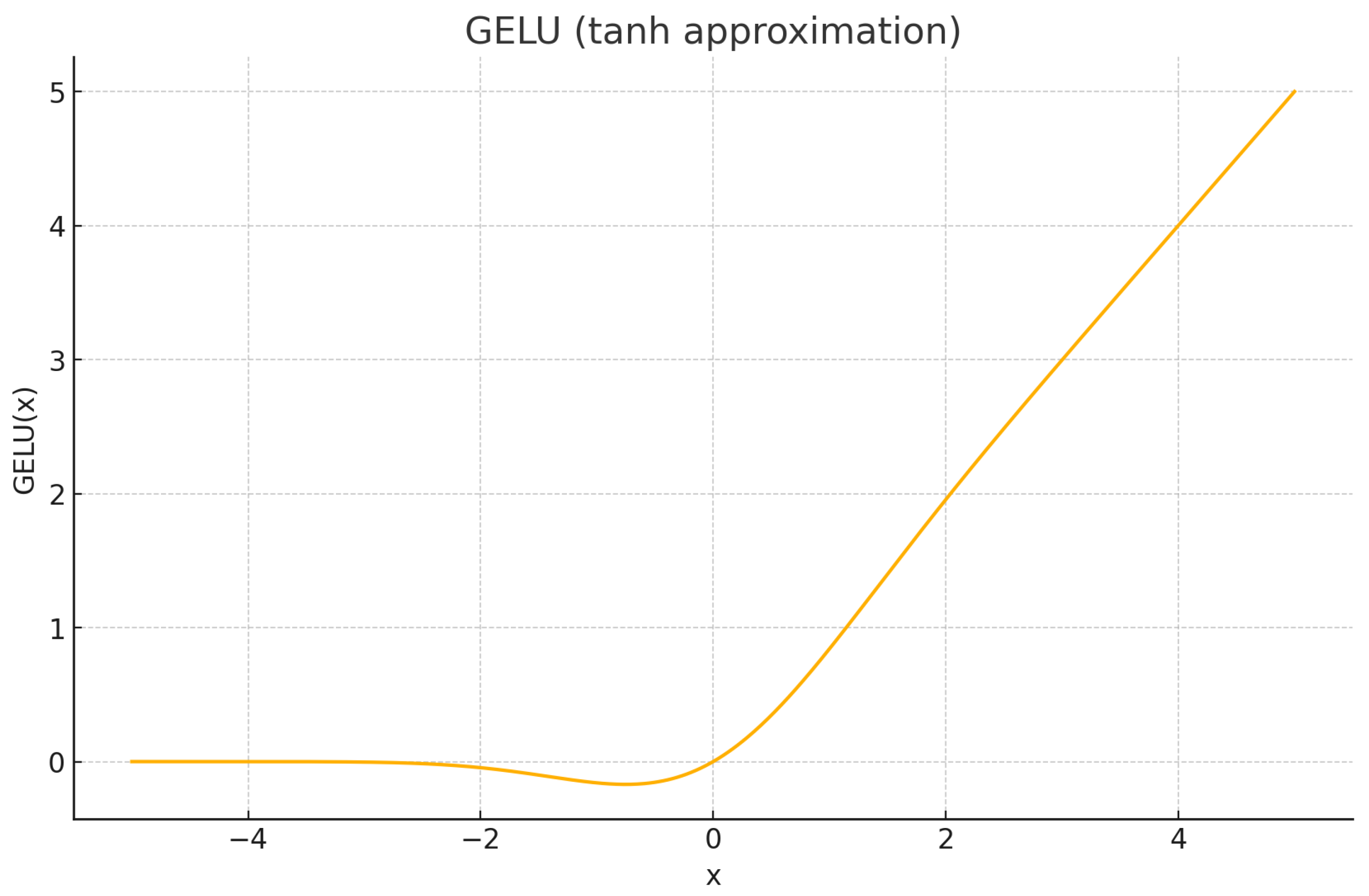
Figure 17.
Graph of Softmax output distributions across three example classes.
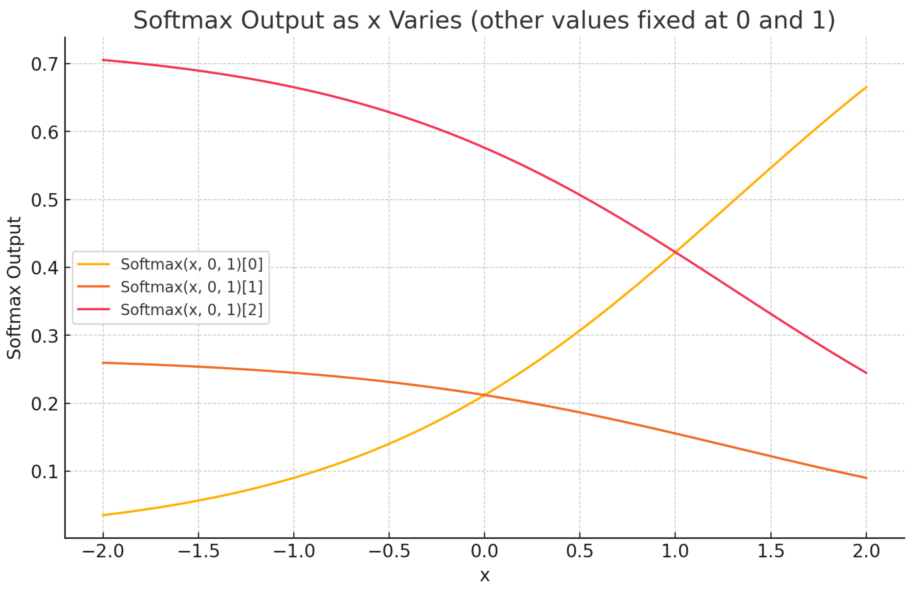
Figure 19.
Overview of a complete image-based machine learning workflow. The process begins with preprocessing and normalization of 100×100 pixel grayscale images, which are then converted into tensors for input into the model. The network includes two hidden layers with Swish activations and Xavier weight initialization, followed by a sigmoid output layer. Adam’s Optimizer guides training via backpropagation, iterating across epochs with periodic logging and batch switching based on convergence thresholds.
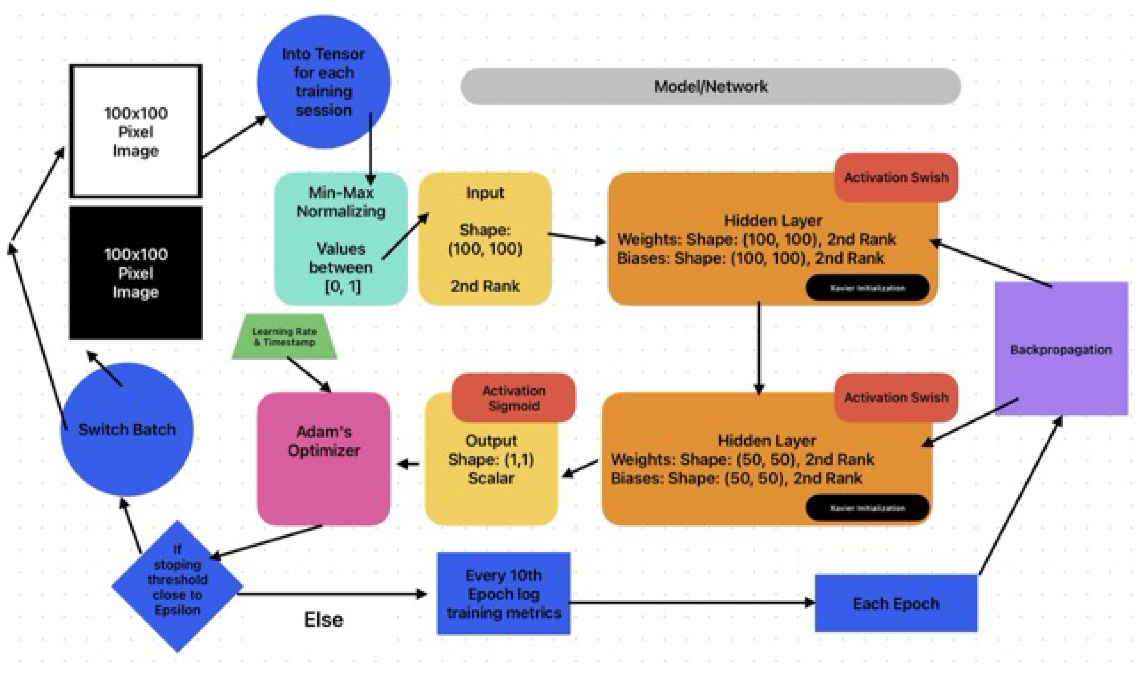
Disclaimer/Publisher’s Note: The statements, opinions and data contained in all publications are solely those of the individual author(s) and contributor(s) and not of MDPI and/or the editor(s). MDPI and/or the editor(s) disclaim responsibility for any injury to people or property resulting from any ideas, methods, instructions or products referred to in the content. |
© 2025 by the authors. Licensee MDPI, Basel, Switzerland. This article is an open access article distributed under the terms and conditions of the Creative Commons Attribution (CC BY) license (http://creativecommons.org/licenses/by/4.0/).
Copyright: This open access article is published under a Creative Commons CC BY 4.0 license, which permit the free download, distribution, and reuse, provided that the author and preprint are cited in any reuse.


