
Submitted:
04 November 2025
Posted:
04 November 2025
You are already at the latest version
Abstract
The ϵ-δ definition of continuity, foundational to real analysis, continues to attract sustained interest across the mathematics community. This paper responds to this interest by providing a comprehensive, systematic survey of direct ϵ-δ proofs for a broad spectrum of functions. We meticulously analyze 54 prominent real-valued functions, categorizing them into eight distinct clusters to highlight recurring proof structures and methodologies. For each function, we present a step-by-step proof alongside an explicit formula for δ in terms of ϵ and the point of continuity. Beyond serving as a robust pedagogical resource for students, instructors, and independent learners, this collection demystifies the proof-writing process by showcasing the elegant, unifying logic underlying a seemingly diverse set of problems. The work’s organized structure and detailed examples offer clarity where confusion often resides, ultimately fostering a deeper intuition for the core principles of continuity. By transforming a collection of challenging proofs into an accessible and navigable reference, this atlas opens up new avenues for further research in the field for mathematicians.
Keywords:
primary: continuity
; secondary: tutorial
; survey
; continuous map
; singular function
; differential calculus
MSC: Primary: 26A15; Secondary: 26-01; 26-02; 54C05; 26A30; 97I40
It is self-evident that any and all paths must be open to a researcher during the actual course of his [or her] investigations. Karl T. W. Weierstrass (1815–-1897)
1. Introduction
The Introduction is structured as follows. Section 1.1 reviews the historical development of – continuity proofs; Section 1.2 presents an up-to-date taxonomy of such proofs; Section 1.3 articulates the motivation and scope of this Atlas; and Section 1.4 concludes the Introduction with a brief roadmap of the paper.
1.1. Historical Background
Early ideas about limits, traceable to Greek mathematicians such as Eudoxus of Cnidus (c. 390–c. 340 BCE) and Archimedes of Syracuse (c. 287–c. 212 BCE), were effective but not rigorously formulated. In the seventeenth century, Sir Isaac Newton (1643–1727) and Gottfried W. Leibniz (1646–1716) developed calculus with the aid of infinitesimals—powerful heuristic quantities that lacked a precise foundation. The demand for rigor intensified in the nineteenth century, as authors such as Augustin-Louis B. Cauchy (1789–1857) sought to recast calculus within the framework of analysis rather than geometry. Bernard P.J.N. Bolzano (1781–1848) sketched ideas akin to the – method as early as 1817, but his work remained largely unnoticed for decades. The decisive step was taken by Karl T.W. Weierstrass (1815–1897), whose mid-nineteenth-century lectures introduced the formal definition of limit and supplied a robust arithmetical basis for continuity and its proofs. The notation was consolidated only later: while variants of “lim” appeared earlier, the now-standard placement of the arrow in was popularized by Godfrey H. Hardy (1877–1947) in 1908 [1,2,3,4,5].
1.2. Taxonomy
To ensure the reader has a clear, structured overview of the material to be presented in this "atlas" of proofs we review the following comprehensive list of taxonomy in epsilon -delta proofs [6,7]:
- Function family (what is f?). Linear/affine; power and root (with domain caveats); polynomials; rational (poles vs. removable points distinguished); exponential and logarithmic; trigonometric and inverse trigonometric; hyperbolic and inverse hyperbolic; absolute value and ; piecewise/defined-by-cases; and selected “pathological” exemplars (Thomae, Weierstrass, Cantor function) where local continuity is instructive.
- Point type (where is continuity checked?). Interior points; boundary points of the domain (one-sided neighborhoods); removable singularities (limit exists and can be defined); and, for contrast, essential/jump points when documenting discontinuity.
- Proof structure (how do we construct ?). The scratch-work ⇒ formal-proof pipeline; backwards–forwards organization; factor–bound–squeeze schemes (e.g., factor , bound a cofactor by C, set ); squeeze and triangle-inequality templates; and contradiction patterns for discontinuity.
- Quantitative strength of continuity. Pointwise continuity (); uniform continuity on a set (); Lipschitz/Hölder cases (explicit such as ); and modulus of continuity with .
- Bounding toolkits (reusable inequalities). Algebraic: , ; power/Bernoulli-type bounds for ; trigonometric bounds , ; elementary exponential/logarithmic bounds; rational bounds via denominator lower bounds on punctured neighborhoods.
- Dependence of on parameters. (i) on a set (uniform continuity); (ii) (continuity at only); (iii) parameterized families : continuity in x at fixed vs. joint continuity in .
- Topological reformulations.–⟺ preimage of open sets is open; sequential characterization (). Recorded for completeness; the atlas emphasizes constructive .
- Role of the function space . Continuity-preserving operators: finite sums/products/scalar multiples/quotients (away from zeros), composition, , absolute value; compact-set principles (e.g., uniform limits preserve continuity); and metrics/topologies on (pointwise vs. uniform) to situate when a single exists. General theorems/schemata are stated here and instantiated by the examples.
- Piecewise construction and junction analysis. (a) Continuity on each piece, (b) existence of one-sided limits at breakpoints, and (c) agreement with the function value.
- Discontinuity taxonomy (for contrast). Removable, jump, and essential discontinuities, including oscillatory counterexamples, to delineate the scope of the methods.
1.3. Motivation and Scope
This Atlas addresses a recurring learning obstacle in early real analysis: students often grasp the idea of continuity but struggle to execute rigorous – arguments in practice. Our aim is to provide a structured collection of direct proofs in the function space that (i) minimize technical overhead, (ii) employ only basic algebra and a short list of standard equalities and inequalities, and (iii) foreground the – definition so that points of genuine difficulty are visible rather than hidden behind broad theorems. The hope is the result to be a curated, self-contained pedagogical-research reference that complements standard textbooks, supports independent study, offers classroom-ready exemplars for instructors, and—by way of a closing section on open problems—engages research mathematicians.
Audience and Objectives
The Atlas is designed for four overlapping audiences: students in their first rigorous analysis course, instructors seeking transparent classroom demonstrations, independent learners, and research mathematicians. Across these groups, our objectives are: (i) to avoid unnecessarily lengthy derivations while preserving full rigor; (ii) to standardize bounding strategies via a small, reusable toolkit of equalities and inequalities; (iii) to highlight how the choice of method influences continuity claims in ; (iv) to build confidence through carefully scaffolded, direct – constructions; and (v) to articulate concise research questions that naturally emerge from the techniques and limitations exhibited by the proofs.
Benefits for Students
As a supplement to a primary textbook, the Atlas offers a practical pathway from definition to proof:
- Direct method first. Each argument begins with the – definition, revealing where the core difficulty arises and how to neutralize it.
- Minimal prerequisites. Proofs rely on basic algebra and a concise catalogue of equalities and inequalities.
- Reusable schemata. Standard proof schemes and patterns (e.g., factor-and-bound, local uniform bounds on cofactors, and “” closures) are made explicit and portable across examples.
- Confidence building. Worked examples progress in difficulty, helping students transition from imitation of templates to independent problem solving.
- Centralized reference. Results that are typically scattered across chapters and sources are presented in one place for quick comparison and review.
Benefits for Instructors
For course designers and lecturers, the Atlas functions as a ready-to-deploy teaching resource:
- Classroom-ready exemplars. Short, fully rigorous proofs suitable for board work or slides, with clearly marked bounding steps.
- Varied demonstrations. Multiple routes to a result (algebraic techniques, alternative equalities, alternative inequalities, or different local bounds) support adaptive instruction.
- Assessment alignment. The proofs decompose naturally into graded checkpoints (e.g., problem framing, bounding choice, construction, and quantifier closure).
- Curricular integration. Side-by-side treatments under different methods and perspectives (e.g., pointwise vs. uniform) make abstract distinctions concrete.
- Economy of time. Concise arguments minimize in-class derivation length without sacrificing logical completeness.
Benefits for Independent Learners
For readers pursuing self-study outside a formal course, the Atlas is organized to support disciplined, incremental mastery:
- Self-paced progression. Topics are sequenced from elementary to advanced, with clearly marked prerequisites and optional extensions.
- Diagnostic checkpoints. Each proof highlights the key steps and decision points (e.g., choice of cofactor g, selection of bounds, calibration of C) to encourage metacognitive practice.
- Template portability. Reusable schemata (e.g., factor-and-bound, local bounding, closure) are summarized for adaptation to new functions.
- Minimal toolkit. Only basic algebra and a compact list of equalities and inequalities are assumed, lowering the barrier to independent entry.
- Cross-Scheme insight. Parallel treatments under different proof schemes and methods promote conceptual transfer beyond single-problem techniques.
Benefits for Mathematicians
Beyond pedagogy, the Atlas surfaces methodological and structural questions:
- Technique extraction. The proofs isolate recurring schemes, steps and bounding moves that may generalize to broader and more abstract classes in and related spaces.
- Metric sensitivity. Side-by-side comparisons under distinct methods and perspectives highlight where continuity is stable and where it fails, suggesting avenues for characterization results.
- Problem generation. Tight bounds, extremal examples, and borderline cases naturally motivate conjectures recorded in the open-problems section.
Pedagogical Benefits
The Atlas advances pedagogical practice by enforcing clarity at each stage of an – proof: the type of proof scheme, the steps and type of applied auxiliary equalities and inequalities. By standardizing these moves, the Atlas reduces cognitive load, exposes the transferable structure of continuity arguments, and lowers barriers to entry for learners who might otherwise be discouraged by fragmented or overly abstract presentations. As a curated collection, it fills an accessibility gap between terse textbook treatments and sprawling online materials.
Research Component and Open Problems
To underscore that this Atlas is a pedagogical–research contribution, it concludes with a section on Open Research Problems. These problems crystallize from the techniques and limitations revealed by the proofs. The intent is to invite further investigation and subsequent publications, thereby connecting classroom clarity with active research directions.
1.4. Outline of the Paper
The paper is organized as follows. Section 2 reviews the necessary preliminaries from college algebra and introductory real analysis that are used in subsequent sections. Section 3 presents the main results: direct – proofs establishing the stability of continuity under finite algebraic operations and proofs across eight clusters of real-valued functions commonly treated in real analysis courses. Section 4 concludes with a discussion of the results, common pitfalls in – arguments, and directions for further advanced research.
2. Preliminaries
Readers who have studied the key topics of college Algebra and elementary real analysis are well-equipped with the following notations, definitions, and results in the areas of "algebraic comparisons" and “continuity” [8,9,10,11].
2.1. Foundations
2.1.1. Definitions
In this subsection we fix notation and recall the classical – formulation of continuity for real-valued functions. Throughout, we emphasize that the admissible may depend on both and the base point [8,9].
Definition 1
(Function Space ). Let denote the set of real numbers. Then, the set of all functions is called the function space This space, equipped with conventional addition + and scalar multiplication · constitutes a vector space.
Remark 1.
To ensure consistency on domains of the discussed functions, for any real-valued function f with domain we extend its definition to entire by defining for all but our focus on its continuity points remains on its points in its original defined domain
Definition 2
(Point Continuity). Let and Then, f is said to be continuous at denoted by if and only if for any given "output tolerance" there exist an "input tolerance" such that for all if then In mathematical logic language:
Remark 2.
In the definition 2, the notation means that δ depends to the given rather than being a function of it. Trivially, any satisfies the condition "" of continuity upon validity of the statement (1).
Remark 3.
In the definition 2, without loss of generality we may assume is sufficiently small enough. Trivially, when the statement (1) holds for shrunken it holds for original epsilon too.
Remark 4.
The contrary to the definition 2 is the concept of discontinuity. Here, f is said to be discontinuous at denoted by if and only if:
Definition 3.
Let with its original definition domain Then, the set of all continuities of f is denoted by the set of discontinuities of denoted by and the set of roots of f are defined by, respectively:
Remark 5.
The set in the Definition 3 is either empty, non-empty finite, denumerable, or uncountable.
Definition 4
(Dirichlet-type functions). Let We classify f according to the size of and as follows:
- Type I Dirichlet function: and .
- Type II Dirichlet function:(for some ) and .
- Type III Dirichlet function: and .
- Type IV Dirichlet function: and .
2.1.2. Proof Workflow and Schemes
Remark 6
(Proof Workflow). A step-by-step guide on how to approach an epsilon-delta proof, includes the typical workflow:
- Given an , find a .
- Start with the inequality and work backward to find a relationship between and ϵ.
- Show that choosing δ based on this relationship guarantees the original inequality holds.
Remark 7
(Proof Scheme I). The first useful process to prove statement (1) in Definition 2 is to begin with and bound it by a factor of : find a function such that
Choose and a constant so that whenever . Then, for any , if we have
which verifies the ϵ–δ condition. Hence we may take:
Remark 8
(Proof Scheme II). The second useful process to prove statement (1) in the definition 2 is to start with the inequality including the expression and find its equivalent inequality including expression that is for some positive bi-variate functions we have:
Now, using Symmetric-anti Symmetric inequality (29) it is sufficient to consider:
Remark 9
(Proof Scheme III). The third useful process to prove statement (1) in the definition 2 is to present the function f as composite where the information on the individual function and in already known. Here, for given since is continuous at there is such that the statement (1) holds. Furthermore, for the found since the function is continuous at there is a such that the statement (1) holds too. Substituting of the value of it follows that for the case of composition function f it is sufficient to consider:
2.2. Auxiliary Equalities and Inequalities
The following list of identities and inequalities play a prominent role in after-mentioned Proof Schema I and Proof Schema II in Remarks 7-8 [10,11].
Notation. Given a sequence of reals We define and
2.2.1. Auxiliary Equalities
We record several identities used throughout the paper.
Lemma 1
(Algebraic and trigonometric identities). Let denote the real numbers. Then:
- General Product Decomposition (GPD).For any integer and elements ,
- Difference of Powers Factorization (DPF).For any and integer ,
- Max/min Recursive.For any
- Max/min via absolute value.For any
- Trigonometric subtraction (sum–to–product).For any
- Hyperbolic subtraction properties.For any
2.2.2. Auxiliary Inequalities
We record several inequalities used throughout the paper.
Lemma 2
(Inequalities used in the sequel). Let , let , and let . Then:
- Generalized triangle inequality.
- Two–Sided Bernoulli Power Bounds(TSBPB).For any and ,
- Reverse triangle inequality.For any
- Symmetric-anti Symmetric inequality.For any and
- Chord–arc bound for sine.For any
- Distance reverse triangle inequality .For any
3. Main Results
3.1. Stability of Continuity Under Algebraic Operations
In real analysis, algebraic operations on continuous functions are typically established by first giving a direct – proof for the binary case , and then extending the statement to general n by mere mathematical induction, while the underlying proof method is left implicit [7,12,13,14,15]. In contrast, in this section we work directly with – estimates for a finite family of functions, proving the continuity of finite sums, finite products, and finite compositions without invoking induction on n. This perspective makes explicit the quantitative bounds (shared ’s, uniform envelopes, and cascaded tolerances) that drive the arguments. Finally, since naively passing from “finite” to “infinite” operations is not valid, we provide counterexamples showing why the finiteness assumptions are essential: infinite sums, products, iterated compositions or maximum (minimum) of continuous functions may fail to define a real-valued function at a point, and even when defined, need not be continuous.
Theorem 1.
Let be real-valued functions, and let . If each is continuous at , then the finite sum is continuous at ; that is,
Proof.
Given Then, by assumption and Definition 2 there are such that for all whenever then Now, define:
Then, we have:
Next, using the General triangle inequality (25), for all whenever it follows that:
This completes the proof. □
Counterexample 3.1.
In Theorem 1, the condition of finite n is necessary. To see the necessity of this restriction, it is sufficient to consider As the harmonic series is divergent, it follows that given by is not a real-valued function and hence discussing its continuity is irrelevant.
Theorem 2.
Let be real-valued functions, and let . If each is continuous at , then the finite product is continuous at ; that is,
Proof.
The proof of the theorem is accomplished in three steps as follows:
Step 1. (Uniform Bound Existence) Let Then, by assumption and Definition 2 there are such that for all whenever then But, the latest statement yields Now, define:
and Then, we have:
Step 2. (Uniform Approximation Existence) Let Again, by assumption and Definition 2 there are such that for all whenever then Now, define:
Then, we have:
Step 3. GPD Application Let Take as defined in Step 1 and Step 2 and given by:
Finally, by an application of GPD (11), for all whenever it follows that:
This completes the proof. □
Counterexample 3.2.
In Theorem 2, the condition of finite n is necessary. To see the necessity of this restriction, it is sufficient to consider As the factorial function diverges to infinity, it follows that given by is not a real-valued function and hence discussing its continuity is irrelevant.
Exercise 3.3.
A modification of above proofs can be applied for the epsilon-delta continuity proof of the following special cases:
- (a)
- the Arithmetic Mean:
- (b)
- the Geometric Mean:
- (c)
- the Harmonic Mean:
Theorem 3.
Let be real-valued functions, and let . If each is continuous at with , then the finite composition is continuous at ; that is,
Proof.
We apply the cascade epsilon-delta method as follows. Since is continuous at , for any given there exists such that:
Now, let be given. Proceeding backward in this way, we obtain tolerances and finally a such that:
Hence, the by considering cascade of implications and given by:
it follows that for all with we obtain . This completes the proof. □
Counterexample 3.4.
In Theorem 3, the condition of finite n is necessary. To see the necessity of this restriction, it is sufficient to consider As the factorial function diverges to infinity, it follows that given by is not a continuous function at
Exercise 3.5.
A similar proof to the above shows that for the continuous function given by is continuous at for any , but not for
Theorem 4.
Let be real-valued functions, and let . If each is continuous at , then the finite maximum is continuous at ; that is,
Proof.
We prove the assertion in two steps as follows:
Step 1. (Upper Bound Existence) Fix Then, for all using equation (13) , (15) and inequality (28) it follows that:
or equivalently:
Next, taking sums on both sides of inequality (45) over it follows that:
Step 2. (The delta Assessment) Given Then, repeating the similar argument as in the proof of Theorem 1, it is sufficient to consider:
This completes the proof. □
Counterexample 3.6.
In Theorem 4, the condition of finite n is necessary. To see the necessity of this restriction, it is sufficient to consider As the sequence of natural numbers is divergent, it follows that given by is not a real-valued function and hence discussing its continuity is irrelevant.
Exercise 3.7.
The twin results for the case of the Minimum function
- (a)
- A modification of above proof for the maximum function can be applied for the epsilon-delta continuity proof of minimum function .
- (b)
- A modification of above counterexample for the maximum function can be applied for the associated counterexample of minimum function .
Remark 10.
In contrast to addition, multiplication and composition, division does not admit a well-defined generalized n-ary form in standard algebra. Specifically, there exists no established algebraic operation or special symbol representing a “generalized division” of functions. This limitation arises from the fact that division is not an associative operation; that is, for functions (or real numbers) , one generally has:
Consequently, the notion of division is inherently restricted to the binary case , where its meaning remains unambiguous.
3.2. Atlas of Epsilon-Delta Continuity Proofs
In this section we present rigorous – continuity proofs for eight clusters of real-valued functions: (i) algebraic [16], (ii) exponential and logarithmic [17,18,19,20,21], (iii) trigonometric [22], (iv) inverse trigonometric [22], (v) hyperbolic [22], (vi) inverse-hyperbolic [22], (vii) elementary piecewise [23,24], and (viii) pathological functions [25,26,27,28,29,30,31,32,33]. Each cluster comprises several special cases, totaling 54 functions. For each case, given and a point of continuity , we provide a sample choice that satisfies the condition in Definition 2. In every proof we apply one of three deduction templates—Proof Scheme I, Proof Scheme II, or Proof Scheme III. Where helpful, we include targeted exercises that invite readers to apply the same methods to closely related instances and thereby deepen their understanding.
3.2.1. Algebraics
Theorem 5.
(Polynomials)Let Then,
Proof.
Fix and given We accomplish the proof in few steps:
Step 1. (Individual Cases) We consider three cases as follows:
Case 1: The case for is trivial by taking
Case 2: The case for is trivial by taking
Case 3: The case for involves the general scheme in Remark 7. First, using DPF equality (12) it follows that:
Set and take so that Then, as the latest bound on x implies it follows that:
Now, it is sufficient to consider
Step 2. (Merging cases) Finally, to combine all three cases, it is sufficient to consider:
This completes the proof. □
Exercise 3.8.
The above proof can be applied for the following special polynomial functions:
- (a)
- the basic form polynomials (constant, linear, quadratic, cubic),
- (b)
- special families of orthogonal polynomials (Legendre, Chebyshev, Hermite, Laguerre, Bernoulli, Euler),
- (c)
- the Cyclotomic polynomials,
- (d)
- the Minimal polynomials,
- (e)
- the Smoothstep function (),
- (f)
- the base Logistic map ().
Theorem 6.
(Powers)Let Then,
Proof.
We accomplish the proof in few steps:
Step 1. (Establishing Reference Case) Reference Case: Fix and given First, when it is sufficient to take Second, we assume We again apply general scheme in Remark 7. First, by two applications of TSBPB inequality (26), () it follows that whenever are defined:
Set and take so that Then, using the reverse triangle inequality (28) it follows that or equivalently Next, two applications of the latest inequality for and , respectively yield:
Accordingly:
Now, it is sufficient to consider:
Step 2. (Case by Case Proofs) Second, we consider two cases as follows:
Case 1: Fix We simply repeat the proof in Reference Case for domain area of .
Case 2: Fix Here, We simply repeat the proof in Reference Case for domain area .
Case 3: Fix Here, we simply repeat the proof in Reference Case for domain area .
This completes the proof. □
Exercise 3.9.
The above proof can be applied for the following special power cases:
- (a)
- the integer powers (e.g., )
- (b)
- the rational powers (e.g., )
Remark 11
(Transcendental Powers). The Reference Case in the proof of Theorem 6 is valid for the special Case as well. Hence,this proof establishes the continuity of the (non-algebraic) transcendental powers too. Some prominent cases include the following:
- (a)
- (b)
- (c)
- (d)
Theorem 7.
(General Rationals)Let Then,
Proof.
Fix with We accomplish the proof in four steps:
Step 1. (Upper Bound Representation) Let and Then:
Step 2. (Upper Bound for Factors) Let Since, q is continuous at there exists such that for all whenever we have: Hence, using the reverse triangle inequality (28) we have This latest inequality yields or equivalently Accordingly, the right hand of inequality (56) has upper bound as in the following:
Step 3. (Neighborhood Approximations) Given Define and By continuity of p and q at there are and such that for all whenever we have and, whenever we have Equivalently:
Step 4. (The delta Assessment). Let Then, combining inequalities (56)-() we have:
This is simplified to:
This completes the proof. □
Exercise 3.10.
The above proof can be applied for the following special rational functions:
- (a)
- the Möbius (linear fractional) functions (),
- (b)
- the Quadratic-over-linear rationals,
- (c)
- the Cubic-over-quadratic rationals,
- (d)
- the Runge function (),
- (e)
- the Hill function ().
3.2.2. Exponential & Logarithmic Family
Proposition 1.
(Logarithm family)Let Then,
Proof.
We accomplish the proof in few steps:
Step 1. (Establishing individual cases) We consider two cases as follows:
Case 1 (): Given and fix Then, for all by a series of algebraic operations we have:
Now, using Symmetric-anti Symmetric inequality (29) it is sufficient to consider
Case 2(): Here, with similar argument as in above it sufficient to consider
Step 2. (Merging cases) Finally, both cases can be combined by considering:
This completes the proof. □
Proposition 2.
(Exponential family)Let Then,
Proof.
We accomplish the proof in few steps:
Step 1.(Establishing individual cases) We consider two cases as follows (Case is trivial):
Case 1 (): Given and fix Then, for all by a series of algebraic operations we have:
Now, using Symmetric-anti Symmetric inequality (29) it is sufficient to consider
Case 2(): Here, with a similar argument to the Case 1 we have,
Step 2. (Merging cases) Finally, both cases can be combined by considering:
This completes the proof. □
Proposition 3.
(Inverse Lambert W function)Let Then,
Proof.
Fix Similar to the proof of Theorem 5, we accomplish the proof in few steps:
Step 1. (Upper Bound Representation) Using GPD equality (11), we have:
Step 2. (Upper Bound for Factor) Let Then, for all with we have Accordingly, the right hand of inequality (70) has upper bound as in the following:
Step 3. (Neighborhood Approximations) Given Define and Then, by continuity of identity function I and the exponential function at there are and such that for all whenever we have and whenever we have Equivalently:
Step 4. (The delta Assessment). Let Then, combining inequalities (70)-() we have:
Finally, using equation (51) for and equation (69) for respectively, we have and respectively. Hence:
This completes the proof. □
Proposition 4.
(The Negative-entropy potential)Let Then,
Proof.
The proof is essentially the repetition of the proof of previous proposition with replaced by and minor changes. First, fix then the inequality (70) is replaced by:
Second, take to obtain an upper bound for factor for all with :
This completes the proof. □
Proposition 5.
(The Tetration function)Let Then,
Proof.
We accomplish the proof in few steps:
Step 1. (Composite representation) We apply the method of the proof of Theorem 3 given the identity for all
Step 2. (Component cascade estimations) Fix and given First, as the function is continuous at we have:
where by the equation (69) for :
Step 3. (Final assessment) Finally, substituting the value of from equation (80) in to equation (82) it follows that:
This completes the proof. □
Proposition 6.
(The Normal density)Let Then,
Proof.
The proof is essentially similar to the proof of previous proposition. Here, we have the identity where and for all Fix and Then, using equation (69) for , and equation (51) for respectively, the corresponding and respectively, are given by:
Finally, substituting the value of from equation (84) in to equation () it follows that:
This completes the proof. □
Proposition 7.
(The Logistic function)Let Then,
Proof.
The proof is essentially similar to the proof of previous proposition too. Here, we have the identity where and for all Fix and Then, using equation (65) for and, equation (69) for respectively, the corresponding and respectively, are given by:
Finally, substituting the value of from equation (87) in to equation () it follows that:
This completes the proof. □
Exercise 3.11.
The above proofs can be applied for the following functions:
- (a)
- the bump function (),
- (b)
- the standard normal density (),
- (c)
- the Softplus function (),
- (d)
- the standard logistic function (),
- (e)
- the logit map ().
Remark 12.
The last three functions in above list are members of the elementary transforms and sigmoids family of functions.
3.2.3. Trigonometrics
Proposition 8.(The Trigonometric functions)Let Then, where
Proof.
Given We prove the continuity as follows:
-
Accordingly, it is sufficient to take:
-
Let and fix By equation () and inequality (30) it follows that:Accordingly, it is sufficient to take:
-
Let and fix First, using equality () and inequality (30) it follows that:Second, set Since is continuous at by equation (93) there is such that for all with we have As before, an application of reverse triangle inequality (28) yields This latest inequality implies or equivalently:Finally, is given by:
-
Let and fix First, using equality () and inequality (30) it follows that:
-
Let and fix First, using equality () and inequality (30) it follows that:
-
Let and fix First, using equality () and inequality (30) it follows that:
This completes the proof. □
Exercise 3.12.
The above proofs can be applied for the following function:
- (a)
- the Haversine function ().
3.2.4. Inverse-Trigonometrics
Proposition 9.
(The Inverse-Trigonometric functions)Let Then,
Proof.
Without loss of generality, we assume the given is sufficiently small such that all quantities of the form are well defined [i.e., ]. We prove the continuity using Remark 8 as follows:
-
Let and fix Then, for all by a series of algebraic operations we have:Now, using Symmetric-anti Symmetric inequality (29) it is sufficient to consider:
-
Let and fix Then, for all by a series of algebraic operations we have:Now, using Symmetric-anti Symmetric inequality (29) it is sufficient to consider:
- Let and fix Then, by similar proof to the case of with sin replaced by tan, and arcsin replaced by arctan, respectively, we have:
- Let and fix Then, by similar proof to the case of with cos replaced by cot, and arccos replaced by arccot, respectively, we have:
- Let and fix Then, by similar proof to the case of with sin replaced by sec, and arcsin replaced by arcsec, respectively, we have:
- Let and fix Then, by similar proof to the case of with cos replaced by csc, and arccos replaced by arccsc, respectively, we have:
This completes the proof. □
Exercise 3.13.
An alternative method to prove continuity of the above inverse trigonometric functions is consideration of the following equations and applying the proof scheme presented in Remark (7):
- (a)
- (b)
- (c)
- (d)
- (e)
- (f)
3.2.5. Hyperbolics
Proposition 10.
(The Hyperbolic functions)Let Then,
Proof.
Given We prove the continuity as follows:
-
Let and fix We accomplish the proof in few steps:Step 1. (Upper Bound Representation). By definition:Step 2. (Neighborhood Approximations). Given Define and By continuity of at the point and, at the point there are and respectively, such that for all whenever we have , and, whenever we have , respectively. Equivalently:Step 3. (The delta Assessment). Let Then, combining inequalities (112)-() we have:Finally, the formula of via two times application of equation (69) for and , respectively, is given by:
- Let and fix Then, given that a similar proof for above presented proof for the case of applies. Hence:
-
Let and fix By definition, and equalities (23), () and lower bound of 1 for the function it follows that:Now, it is sufficient to take:Then, by (118) we have:
-
Let and fix By definition, and lower bound of 1 for the function it follows that:So any that makes also makes . In this way the continuity of sech at is “dominated’’ by (indeed, follows from) the continuity of cosh at . Hence, it is sufficient to take:
-
Let and fix We accomplish the proof in few steps:Step 1.(Upper Bound Representation). By definition and equalities (23), ():Step 2.(Neighborhood Approximation). Set Since is continuous at , by equation (116) there is such that for all with we have As before, an application of reveres triangle inequality (28) yields This latest inequality implies or equivalently:Step 3. (The delta Assessment). Combining the equality (123) and inequality (124), and considering for all with we have:Finally, is given by:
-
Let and fix The proof is essentially similar to he previous proof with some minor modifications as follows. First, the equation (123) is replaced by:Second, for the same and inequality (124) holds. Third, considering for all with we have:Finally, is given by:
This completes the proof. □
3.2.6. Inverses-Hyperbolics
Proposition 11.
(The Inverse-Hyperbolic functions)Let Then,
Proof.
For each case below, fix small enough so that the perturbed arguments remain in the domain of the corresponding direct map (e.g., for arcosh, arsech require ; for arcoth, arcsch require and to stay on the same branch). The proof schema is using Remark 8 similar to that of Inverse-Trigonometric functions. The list of functions and their corresponding ’s are as follows:
This completes the proof. □
Exercise 3.14.
An alternative method to prove continuity of the above inverse hyperbolic functions is consideration of the following equations and applying the proof scheme presented in Remark (7):
- (a)
- (b)
- (c)
- (d)
- (e)
- (f)
3.2.7. Elementary Piecewise functions
Proposition 12.
(The Elementary Piecewise functions)Let Then,
Proof.
Given We prove the continuity as follows:
-
Let and fix Using Reverse triangle inequality (28) we have:Accordingly, by (136) it is sufficient to set:
-
Accordingly, by (138) it is sufficient to set:
-
Let fix Then, using equality ( ) and inequality (28) and similar to the process above, we have:Accordingly, by (140) it is sufficient to set:
-
Accordingly, by (142) it is sufficient to set:
-
Let fix Set Then:Next, from inequality (144), it follows that if then , and, if then Hence, in both cases or equivalently: Consequently, it is sufficient to set:
-
Let fix Set Then:Next, from inequality (146), it follows that or equivalently Consequently, it is sufficient to set:
-
Let fix Set Then:Next, from inequality (148), it follows that or equivalently Consequently, it is sufficient to set:
-
Let fix Using triangle inequality we have:Next, for all whenever we have and whenever we have respectively. Hence, it is sufficient to take to ensure the right hand side of inequality (150) is less than Finally:
This completes the proof. □
Exercise 3.15.
The modification of above proofs can be applied for the following functions:
- (a)
- the Rectified Linear Unit function (),
- (b)
- (c)
- ),
- (d)
- ),
- (e)
- (f)
- (g)
- the Heaviside function: (),
- (h)
- the Indicator function: (),
- (i)
- the Sawtooth norm: (),
- (j)
- the Tent map: (,
- (k)
- the Sawtooth wave function: ( ),
- (l)
- ,
- (m)
- ,
- (n)
- the Rect(boxcar) kernel: (,
- (o)
- ).
Remark 13.
The last six functions in above list are members of waves.
3.2.8. Pathologic Functions
Proposition 13.(The Volterra-type power–sine family functions)Let Then,
Proof.
Given We prove the continuity as follows:
-
Let and fix First, when it is sufficient to consider Second, assume We accomplish the proof in few steps.Step 1.(Upper Bound Representation). Using inequality (30) it follows that:Step 2. (Neighborhood Approximation). Set and By continuity of the functions and at point respectively, there are and such that for all whenever we have and whenever we have respectively. Equivalently:Step 3. (The delta Assessment). Let . Then, combining inequalities (152)-() we have:Finally, the formulae of via two times application of equation (55) for and respectively is given by:
-
Let and fix Then, using inequality (30) it follows that:Hence, by an application of equation (55) for it is sufficient to consider:
This completes the proof. □
Proposition 14.
(The Cantor function)Let Then,
Proof.
Given Fix We accomplish the proof in few steps as follows:
Step 1.(Key prefix–tail bounds (from the formula)) Set and Then:
- Exact prefix match: If , then:
-
Adjacent prefix (first difference at position n): If the first index where differ is n (so the first digits agree), then:(Worst case: one side contributes a “first-1 spike” plus a tail .)
Step 2.(Turning closeness in x into a prefix agreement) Partition into level-n triadic intervals (“cylinders”) determined by the first n ternary digits. If , then x and lie either
- in the same level-n cylinder (first n digits agree), or
- in adjacent level-n cylinders (first digits agree and they differ at digit n).
Therefore, for all with :
Step 3.(The delta Assessment) Choose: and set Then, whenever , we are in one of the two cases above, so Hence, it is sufficient to consider:
This completes the proof. □
Proposition 15.
(The Thomae function)Let Then,
Proof.
Given and without loss of generality we assume We accomplish the proof in two steps as follows:
Step 1. (Filter the “big spikes” = small denominators) Fix Consider the highest values of candidate set of Here, for any we have So, if we consider a neighborhood of such that the set is removed, we will prove the statement.
Step 2 (Punch a small hole around that misses those spikes) Define:
Then, for all whenever we have the following cases:
Case 1: Fix Then,
Case 2: Fix Then, and (Otherwise, if then yielding a contradiction !). Accordingly,
This completes the proof. □
Proposition 16.
Proposition 16.(The Riemann function)Let Then,
Proof.
Given Fix We accomplish the proof in few steps as follows:
Step 1.(Upper Bound Representation) First, using inequality (90), for any we have Hence:
Note that is granted by setting such that
Step 2. (Upper Bounds for Components) Second, we find an upper bound in terms for each component in the right hand side of inequality (164). Here, the first component is bounded as in:
Next, let satisfy and for all consider the bins of positive integers . Accordingly:
Finally, using upper bound in inequality (167) it is sufficient to consider:
This completes the proof. □
Proposition 17.
(The Takagi function)Let Then,
Proof.
Given Fix We accomplish the proof in few steps as follows:
Step 1.(Upper Bound Representation) First, using inequality (31) and bounds for any we have:
Step 2. (Upper Bounds for Components) Second, using the right hand side components in inequality (169), for we have Furthermore, for whenever we have
Step 3.(The delta Assessment) Finally, from previous step, substituting N in the , the is given by:
This completes the proof. □
Proposition 18.
(The Weierstrass function)Let Then,
Proof.
Given Fix We accomplish the proof in few steps as follows:
Step 1.(Upper Bound Representation) First, using equality () and inequality (30), respectively, for any we have Hence:
Step 2.(Neighborhood Approximation). Set Then, for for all whenever we have or equivalently:
Step 3.(The delta Assessment) Finally, by inequalities (171) and (172) it is sufficient to consider:
This completes the proof. □
Proposition 19.
(The Type I Dirichlet function)Let Then,
Proof.
Given Without loss of generality we may assume Fix We accomplish the proof in few steps as follows:
Step 1. (Restriction of Discussion Domain). Given that has period and for we have it is sufficient to assume
Step 2. (Proof by Contradiction) Assume there is such that for all whenever we have We consider two separate cases as follows:
Case 1: Assume Then, consider the unique base 10 representation where for all Take the rational number Then:
But, a contradiction.
Case 2: Assume Take the irrational number Then:
But, again a contradiction.
This completes the proof. □
Proposition 20.
(The Type II Dirichlet function)Let Then,
Proof.
Given Fix We consider two distinct cases as follows:
Case 1: Assume for some Then, using equation (51) it is sufficient to consider:
Case 2: Assume for all Define and let Since, is continuous at there exists such that for all whenever we have: Hence, using the reverse triangle inequality (28) we have This latest inequality yields and, furthermore:
Finally, it is sufficient to repeat the slightly modified version of the proof in Proposition 19 for the function on the neighborhood to ensure discontinuity at the point .
This completes the proof. □
Proposition 21.
(The Type III Dirichlet function)Let Then,
Proof.
Given Fix We consider two distinct cases as follows:
Case 2: Assume for all Then, it is sufficient to consider and repeat the similar argument to the one in the proof of Proposition 20 to ensure discontinuity at the point
This completes the proof. □
Proposition 22.
(The Type IV Dirichlet function)Let be defined on the closed unit interval by :
where and are defined by a unique sequence of digits by and respectively for all . Then, where C is the classical ternary Cantor-set.
Proof.
Given Fix We consider two distinct cases as follows:
Case 1: Assume with base-3 representation Then, by definition, for all Hence, We modify the proof of Proposition 14 as follows:
Step 1.(Key prefix–tail bounds (from the formula)) Set and Then:
- Exact prefix match: If , then:
-
Adjacent prefix (first difference at position n): If the first index where differ is n (so the first digits agree), then:( Key point: intervals donotpile up; for each x only the first deletion level contributes, which is why the bounds are exactly and .)
Step 2.(Turning closeness in x into a prefix agreement) Partition into level-n triadic intervals (“cylinders”) determined by the first n ternary digits. If , then x and lie either
- in the same level-n cylinder (first n digits agree), or
- in adjacent level-n cylinders (first digits agree and they differ at digit n).
Therefore, for all with :
Step 3.(The delta Assessment) Choose: and set Then, whenever , we are in one of the two cases above, so Hence, it is sufficient to consider:
Case 2: Assume Then, it is sufficient to consider for some and repeat the similar argument to the one in the proof of Proposition 20 to ensure discontinuity at the point
This completes the proof. □
Exercise 3.16.
Given Assume for some continuous function we have for all Using presented ideas in the proofs of above Dirichlet type functions it follows that:
- (a)
- f is type I Dirichlet function whenever
- (b)
- f is type II Dirichlet function whenever (for some ),
- (c)
- f is type III Dirichlet function whenever
- (d)
- f is type IV Dirichlet function whenever
4. Discussion
4.1. Summary and Contributions
This work offers a survey of direct – continuity proofs across eight clusters of real-valued functions, encompassing 54 representative functions. Table 1 presents summary of all related results. It also develops direct – proofs for finite algebraic operations—sum, product, composition and maximum (minimum)—on a prescribed collection of n functions . A notable feature of the exposition is its reliance on only minimal auxiliary results (elementary equalities and inequalities) and basic facts about infinite series, deliberately avoiding advanced theorems and their corollaries.
Taken together, these contributions reinforce the central role of – arguments in (i) teaching the foundations of real analysis and (ii) motivating further mathematical research in this area.
4.2. Common Pitfalls
Common pitfalls arise frequently in – proofs. We highlight several below.
- Treating scratch work as a finished proof. Scratch work often contains tentative guesses—chains of equalities and inequalities relating and —some of which are unsuitable or too advanced for the final argument. For example, for one might invoke the Mean Value Theorem (MVT) to deduce . At the level considered here, however, the MVT is beyond the intended toolkit (which is limited to elementary algebraic identities, inequalities, and basic series facts). Our Appendix provides classroom aids designed to reinforce the structure of a complete and correct written proof.
- Treating as a unique function of . By definition, depends on the prescribed , but it need not be unique: any smaller also suffices. Moreover, continuity at a point typically yields , reflecting dependence on both the tolerance and the base point.
- Ignoring the function’s domain. The definition requires x and to lie in the domain . This is often overlooked. A practical remedy—adopted in this paper—is to extend f to when convenient, while explicitly formulating pointwise continuity with respect to the points in the original domain .
- Algebraic slips. Errors in algebraic manipulation (equalities or inequalities) can invalidate the inferred relationship between and . A final pass checking each logical implication in the chain of estimates is essential.
- Assuming a unique proof. The definition of continuity neither requires nor favors a single method. Our presentation provides one admissible construction among many. Alternative approaches can yield different, equally valid ’s. For instance, for one may start from the auxiliary identity:which leads to a distinct but legitimate – development.
4.3. Future Work and Open Research Problems
Up to this point, we have reviewed and consolidated – continuity proofs for 54 prominent real-valued functions in mathematical analysis. A natural question for the curious reader is whether there remains scope for inquiry beyond the exercises presented here. To the best of the author’s knowledge, the answer is yes: there is room to move beyond the exercise tier and into genuine research. In particular, two principal families of open problems invite further investigation by interested mathematicians, as outlined below.
4.3.1. Point Continuity
First, let be a real-valued function and given Fix and define:
It is trivial that if and only if In this paper, we gave one sample example of elements of for 54 prominent functions in real-analysis presented in Table (Table 1). Now, we consider the following new quantity:
Definition 5.
Let be a real-valued function and given Fix and define:
We present two examples as follows. First, for given and we have Second, for given and we have These examples motivates the following set of Open Problems:
Research Problem 4.1.Compute for all 54 functions presented in Table (Table 1).
Research Problem 4.2.Establish finiteness conditions on as follows:
- What is the necessary condition for f and such that ?
- What is the sufficient condition for f and such that ?
- Is there a necessary and sufficient condition for f and such that ?
4.3.2. Uniform Continuity
Second, consider an stronger version of the concept of "Point Continuity" presented in Definition (2) called "Uniform Continuity" as in follows [34,35]:
Definition 6
(Uniform Continuity). Let Then, f is said to be uniform continuous in its domain if and only if for any given "output tolerance" there exists an "input tolerance" such that for all and for all if then In mathematical logic language:
We present two examples as follows. First, for given we have Second, for given we have These examples motivate the following Open Problem:
Research Problem 4.3.Compute for all 54 functions presented in Table (Table 1).
Next, similar to the case of "Point Continuity", for given and we define:
and, consequently, the following "twin" of Definition (5) for the case of "Uniform Continuity":
Definition 7.
Let be a real-valued function and given Set:
Here, for the same presented examples and we have and Similar to the "Core Continuity" these examples motivates the following set of Open Problems:
Research Problem 4.4.Compute for all 54 functions presented in Table (Table 1).
Research Problem 4.5.Establish finiteness conditions on as follows:
- What is the necessary condition for f such that ?
- What is the sufficient condition for f such that ?
- Is there a necessary and sufficient condition for f such that ?
Conclusion
To synthesize this paper contributions into a single picture—and to orient prospective investigations—we conclude with a guiding metaphor for the reader’s path through the paper. We invite the reader to view the journey through this paper as a deliberate ascent of the south side of mount Everest (see Figure 1). Beginning from the Base Camp of Introduction at the valley floor with elevation , the route first threads the glacier of Camp 1 of Preliminaries with elevation , where footing is secured and the essential tools are checked. The climb then rises to Main Results (3.1), our Camp 2 at , the moment at which technique turns into practice: here the reader enters an Exercise Zone with a clear vista of how to work the proofs and, with steady effort, to traverse toward the Nuptse outcrop at in the follow up route. The ridge continues to the Camp 3 of the Main Results (3.2), where the atlas of – arguments is stitched together like fixed lines up a steep face. By the time one reaches to Camp 4 of Discussion, around , there is room for reflection and route-finding—an earned pause to decide which lines of inquiry to follow next. Above lies the Research Zone, where oxygen is thin but ideas are sharp, and choices about problems and methods become decisive. Some climbers will push to the highest summit—Everest at —by resolving open questions raised by the atlas. Others may traverse to the neighboring Lhotse at , consolidating significant advances on closely related themes. Either outcome is a genuine summit: both routes demand judgment, persistence, and the careful use of the techniques developed below. If you have read to this point, you have already climbed high; what remains is to choose your line and continue upward. May the maps, fixed points, and waymarks provided here make the remaining ascent not only possible, but memorable.
Funding
This research received no external funding.
Institutional Review Board Statement
Not Applicable.
Informed Consent Statement
Not Applicable.
Data Availability Statement
Not Applicable.
Acknowledgments
The author is grateful to his mathematics instructors and to the authors of the textbooks that shaped his understanding of real analysis. Their clarity, rigor, and generosity of exposition guided the development of this work. The author dedicates this paper to their memory with deep respect and appreciation.
Conflicts of Interest
The author declares no conflicts of interest.
Abbreviations
The following abbreviations are used in this manuscript:
Appendix A. Classroom Aids: ϵ-δ Continuity Toolkit
This Appendix provides ready-to-use “Classroom Aids” that scaffold – continuity proofs from first principles [36,37,38,39,40]. The toolkit includes a fully worked worksheet (illustrated for ), a concise analytic rubric that operationalizes proof quality (bounding strategy, explicit construction, and quantifier discipline), and three concept questions for rapid formative assessment. Each aid emphasizes a transferable pattern—introduce an auxiliary radius to freeze cofactors, derive a bound, and choose —with any domain restrictions made explicit. Instructors can adapt the same template verbatim to other prominent functions in real analysis.
Appendix A.1. Worksheet (Fully Worked Example: f(x)=x π :π=3.14159…)
Domain and goal.
Let . Work on the natural real domain
Fix . Prove, by the – definition, that is continuous at any . Here, we want to prove that for every there exists such that
Step 1 (Algebraic bound via TSBPB).
By the Two–Sided Bernoulli Power Bounds for and ,
Impose the auxiliary radius
Hence
Therefore, under we have the linear control
Step 2 (ϵ-δ planning).
It suffices to force
Step 3 (Candidate δ).
Take
Step 4 (Verification).
If and , then in particular , so Step 1 yields
As was arbitrary, is continuous at on .
Quantifier audit.
Instructor note (transfer pattern). The technique generalizes: factor the difference, impose a local radius (often 1) to bound the “cofactor,” then choose . Students should explicitly (i) introduce the auxiliary bound (here, ), (ii) box the candidate , and (iii) complete the quantifier audit. Here, the factorization is done via the the TSBPB bound Keep the same auxiliary radius to freeze the cofactor, then choose The domain restriction to is essential for real-valued .
Appendix A.2. Analytic Rubric (Short Form; 10 Points)
| Criterion | Exceeds / Meets / Not Yet (pts) |
| Problem framing (2pts) | Correct domain identified; precise target for at . Exceeds (2pts): domain stated and goal restated; Meets (1pts): generally correct; NY (0pts): missing/misstated. |
| Bounding strategy (3pts) | Invokes TSBPB (case ) to obtain and justifies a local bound . Exceeds (3pts): fully justified; Meets (2pts): idea present with minor gaps; NY (0–1pts): incorrect or unjustified. |
| construction (3pts) | Gives explicit with . Exceeds (3pts): correct, boxed, and motivated; Meets (2pts): correct but thinly justified; NY (0–1pts): incorrect/implicit. |
| Quantifiers & closure (2pts) | Final implication verified and quantifiers audited. Exceeds (2pts): explicit audit; Meets (1pts): verification present; NY (0pts): omitted. |
Feedback keys for common issues. (i) Domain slip: ensure ; (ii) Unjustified cofactor bound: explicitly state and derive ; (iii) Quantifier order: keep “ in ”.
Appendix A.3. Concept Questions (Peer Instruction/Clickers)
Each question is designed for a 1–2 minute vote, 2–3 minute peer discussion, and a brief plenary debrief.
Q1 (Bounding the cofactor for x π ).
Let . Which line correctly justifies a bound on the cofactor in the TSBPB estimate?
- (a)
- Assume , then , hence
- (b)
- Assume , then .
- (c)
- ; no auxiliary bound is needed.
- (d)
- Replace TSBPB by for all .
Q2 (Selecting δ).
With the setup above, which works?
- (a)
- (b)
- (c)
- (d)
Q3 (Quantifier sensitivity).
Which rephrasing preserves the correct quantifier order for continuity at on ?
- (a)
- for all ).
- (b)
- ).
- (c)
- ).
- (d)
- such that the implication holds for all .
Instructor key. Q1: (a). Q2: (b). Q3: (b).
Adaptation notes. The same template applies to any fixed on by replacing with r and with .
References
- Sinkiewicz, G. I. (2016). On History of Epsilontics. Antiquitates Mathematicae, 10(1), 183–204. [CrossRef]
- Grabiner, J. V. (1983). Who Gave You the Epsilon? Cauchy and the Origins of Rigorous Calculus. The American Mathematical Monthly, 90(3), 185–194. [CrossRef]
- Felscher, W. (2000). Bolzano, Cauchy, Epsilon, Delta. The American Mathematical Monthly, 107(9), 844–862. [CrossRef]
- Burton, D. M. (1997). The History of Mathematics: An Introduction (3rd ed.). New York, USA: McGraw–Hill. ISBN: 978-0-07-009465-9.
- Hardy, G. H. (1921). A Course of Pure Mathematics (3rd ed.). Cambridge, UK: Cambridge University Press. ISBN: 0521720559.
- Pugh, C. C. (2015). Real Mathematical Analysis (3rd ed.). Undergraduate Texts in Mathematics. Switzerland: Springer International Publishing. ISBN: 978-3-319-17770-0.
- Bartle, R. G., & Sherbert, D. R. (2011). Introduction to Real Analysis (4th ed.). Hoboken, NJ, USA: John Wiley & Sons, Inc. ISBN: 978-0-471-43331-6.
- Silverman, R. A. (1985). Calculus with Analytic Geometry. New Jersey, USA: Prentice-Hall, Inc. ISBN: 0-13-111634-7.
- Lin, S.-Y. T., & Lin, Y.-F. (1981). Set Theory with Applications (2nd ed.). Tampa, FL, USA: Mariner Publishing Company. ISBN: 964-01-0462-0.
- Hardy, G. H., Littlewood, J. E., & Pólya, G. (1952). Inequalities (2nd ed.). Cambridge, UK: Cambridge University Press. ISBN: 0521052068.
- Mossaheb, G. H. (1999). Analize Riazi: Teoriye A’dade Haghighi [Mathematical Analysis: Theory of Real Numbers] (Vol. 1). Tehran, Iran: Amirkabir Publication. ISBN: 964-00-0630-0. (In Persian).
- Abbott, S. (2015). Understanding Analysis (2nd ed.). Undergraduate Texts in Mathematics. New York, USA: Springer. ISBN: 978-1-4939-2711-1.
- Tao, T. (2016). Analysis I (3rd ed.). Texts and Readings in Mathematics. New Delhi/Singapore: Hindustan Book Agency / Springer, India. ISBN: 978-93-80250-64-9.
- Botelho, F. S. (2018). Real Analysis and Applications. Cham, Switzerland: Springer International Publishing. ISBN: 978-3-319-78630-8.
- Loeb, P. A. (2016). Real Analysis. Switzerland: Birkhäuser / Springer International Publishing. ISBN: 978-3-319-30742-8.
- Knopp, K. (1996). Algebraic Functions. In Theory of Functions, Parts I and II (pp. 119–134). New York: Dover Publications.
- Bronstein, M. , Corless, R. M., Davenport, J. H., & Jeffrey, D. J. (2008). Algebraic properties of the Lambert W function from a result of Rosenlicht and of Liouville. Integral Transforms and Special Functions 19(10), 709–712. [CrossRef]
- Frigg, R. , & Werndl, C. (2011). Entropy – A Guide for the Perplexed. In C. Beisbart & S. Hartmann (Eds.), Probabilities in Physics (pp. 115–142). Oxford, UK: Oxford University Press.
- Hooshmand, M. H. (2006). Ultrapower and ultraexponential functions. Integral Transforms and Special Functions, 17(8), 549–558. [CrossRef]
- Harris, F. E. (2014). Probability and Statistics. In F. E. Harris (Ed.), Mathematics for Physical Science and Engineering (pp. 663–709). Academic Press. ISBN: 9780128010006. [CrossRef]
- Verhulst, P.-F. (1838). Notice sur la loi que la population poursuit dans son accroissement. Correspondance Mathématique et Physique, 10, 113–121. (French; PDF, retrieved October 26, 2025).
- Oldham, K. B., Myland, J., & Spanier, J. (2009). An Atlas of Functions: withEquator, the Atlas Function Calculator (2nd ed.). New York, NY, USA: Springer. Hardcover ISBN: 978-0-387-48806-6.
- Knuth, D. E. (1997). The Art of Computer Programming, Volume 1: Fundamental Algorithms (3rd ed.). Reading, MA: Addison–Wesley Longman. ISBN: 0-201-89683-4.
- Graham, R. L., Knuth, D. E., & Patashnik, O. (1989). Concrete Mathematics: A Foundation for Computer Science. Reading, MA: Addison–Wesley Publishing Company. xiii+625 pp. ISBN: 0-201-14236-8.
- Ponce-Campuzano, J. C., & Maldonado-Aguilar, M. Á. (2015). Vito Volterra’s construction of a nonconstant function with a bounded, non-Riemann integrable derivative. BSHM Bulletin: Journal of the British Society for the History of Mathematics, 30(2), 143–152. [CrossRef]
- Soltanifar, M. Some Results on the Variation of Composite Function of Functions of Bounded Variation. American Journal of Undergraduate Research, 6(4). [CrossRef]
- Dovgoshey, O. , Martio, O., Ryazanov, V., & Vuorinen, M. (2006). The Cantor function. Expositiones Mathematicae 24(1), 1–37. [CrossRef]
- Beanland, K. (2009). Modifications of Thomae’s function and differentiability. The American Mathematical Monthly, 116(6), 531–535. [CrossRef]
- Weisstein, E. W. (2025). Weierstrass Function. From MathWorld—A Wolfram Resource. https://mathworld.wolfram.com/WeierstrassFunction.html. Accessed: 2025-10-26.
- Hata, M. , & Yamaguti, M. (1984). The Takagi function and its generalization. Japan Journal of Applied Mathematics 1, 183–199. [CrossRef]
- Weierstrass, K. (1895). Über continuirliche Functionen eines reellen Arguments, die für keinen Werth des letzteren einen bestimmten Differentialquotienten besitzen. In Mathematische Werke von Karl Weierstrass (Vol. 2, pp. 71–74). Berlin: Mayer & Müller. (German; English trans.: On continuous functions of a real argument which possess a definite derivative for no value of the argument.
- Lejeune Dirichlet, P. G. (1829). Sur la convergence des séries trigonométriques qui servent à représenter une fonction arbitraire entre des limites données. Journal für die reine und angewandte Mathematik, 4, 157–169. (French).
- Soltanifar, M. (2023). A Classification of Elements of Function Space F(R,R). Mathematics, 11(17), Article 3715. [CrossRef]
- Hernández, C. A. (2015). Epsilon–delta proofs and uniform continuity. Lecturas Matemáticas, 36(1), 23–32.
- Hernández Melo, C. A., & Hernández, F. D. de M. (2019). Uniform Continuity: Another Way to Approach This Concept in the Classroom. The College Mathematics Journal, 50(1), 54–57. [CrossRef]
- Ambrose, S. A., Bridges, M. W., DiPietro, M., Lovett, M. C., & Norman, M. K. (2010). How Learning Works: Seven Research-Based Principles for Smart Teaching. Jossey-Bass.
- Chi, M. T. H. , & Wylie, R. (2014). The ICAP framework: Linking cognitive engagement to active learning outcomes. Educational Psychologist, 49, 219–243. [CrossRef]
- Mazur, E. (1997). Peer Instruction: A User’s Manual. Upper Saddle River, NJ: Prentice Hall.
- Freeman, S. , Eddy, S. L., McDonough, M., Smith, M. K., Okoroafor, N., Jordt, H., & Wenderoth, M. P. (2014). Active learning increases student performance in science, engineering, and mathematics. Proceedings of the National Academy of Sciences 111(23), 8410–8415. [CrossRef]
- Deslauriers, L. , McCarty, L. S., Miller, K., Callaghan, K., & Kestin, G. (2019). Measuring actual learning versus feeling of learning in response to active learning. Proceedings of the National Academy of Sciences 116(39), 19251–19257. [CrossRef]
Figure 1.
Everest analogy for the paper’s structure: the route begins at Introduction, traverses the glacier of Preliminaries, reaches Camp 2 at (Main Results 3.1), climbs to (Main Results 3.2), pauses near (Discussion), and enters the Research Zone, with summits at Everest () and Lhotse ().
Figure 1.
Everest analogy for the paper’s structure: the route begins at Introduction, traverses the glacier of Preliminaries, reaches Camp 2 at (Main Results 3.1), climbs to (Main Results 3.2), pauses near (Discussion), and enters the Research Zone, with summits at Everest () and Lhotse ().
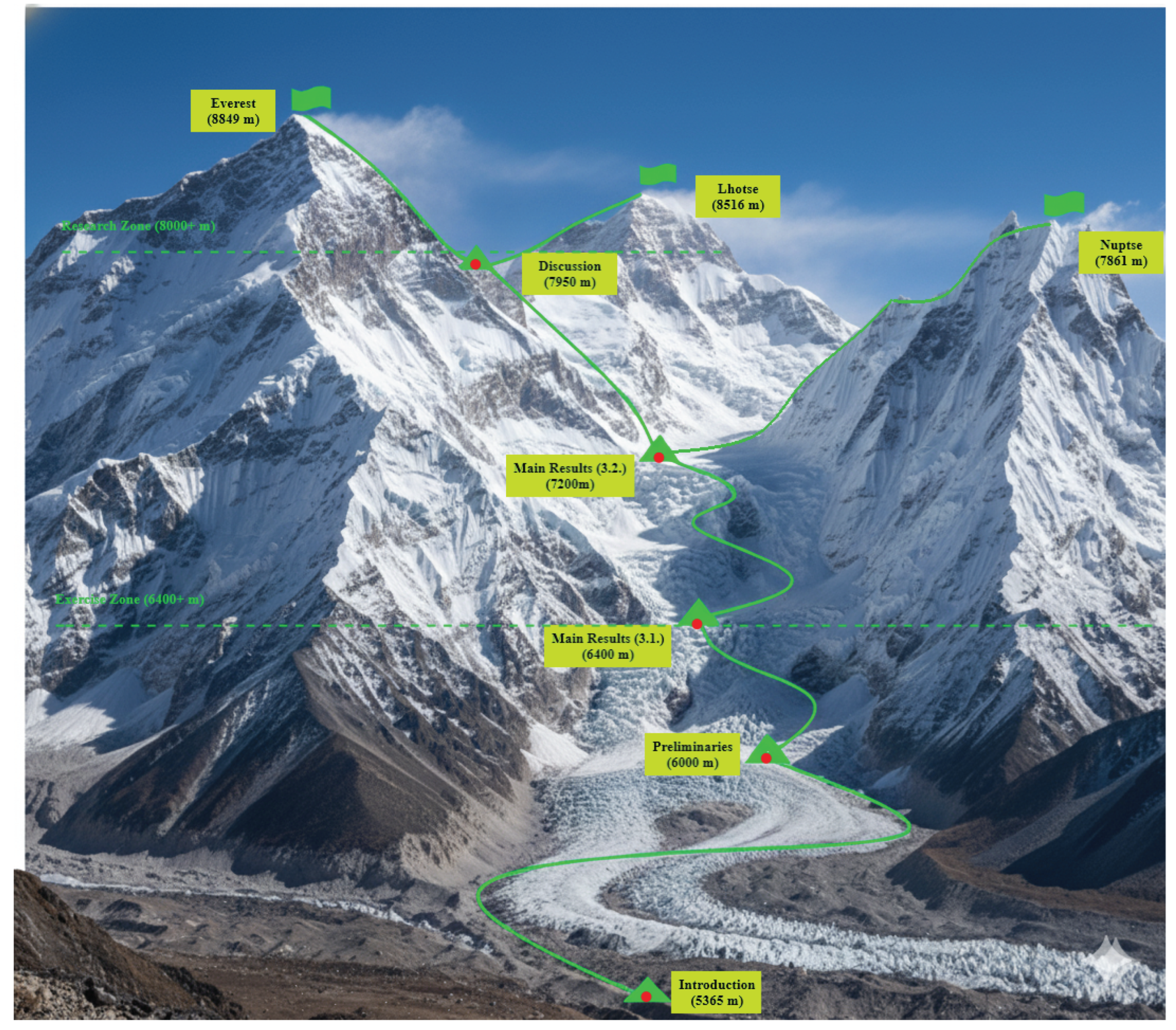

Table 1.
Summary of prominent real valued functions and associated for their continuity at point .
| # | Cluster | Sample |
|---|---|---|
| –Function () | ||
| 1 | Algebraics | |
| 1-1 | —Polynomials | |
| 1-2 | —Powers | |
| 1-3 | —General Rationals | |
| 2 | Exponential and Logarithmic | |
| 2-1 | —Logarithm | |
| 2-2 | —Exponential | |
| 2-3 | —Inverse Lambert | |
| 2-4 | —Neg. Entropy Potential | |
| 2-5 | —Tetration | |
| 2-6 | —Normal density | |
| 2-7 | —Logistic | |
| 3 | Trigonometric | |
| 3-1 | —Trig 1 | |
| 3-2 | —Trig 2 | |
| 3-3 | —Trig 3 | |
| 3-4 | —Trig 4 | |
| 3-5 | —Trig 5 | |
| 3-6 | —Trig 6 | |
| 4 | Inverse-Trigonometric | |
| 4-1 | —Inv-Trig 1 | |
| 4-2 | —Inv-Trig 2 | |
| 4-3 | —Inv-Trig 3 | |
| 4-4 | —Inv-Trig 4 | |
| 4-5 | —Inv-Trig 5 | |
| 4-6 | —Inv-Trig 6 | |
| 5 | Hyperbolic | |
| 5-1 | —Hyperb 1 | |
| 5-2 | —Hyperb 2 | |
| 5-3 | —Hyperb 3 | |
| 5-4 | —Hyperb 4 | |
| 5-5 | —Hyperb 5 | |
| 5-6 | —Hyperb 6 | |
| 6 | Inverse-Hyperbolic | |
| 6-1 | —Inv-Hyperb 1 | |
| 6-2 | —Inv-Hyperb 2 | |
| 6-3 | —Inv-Hyperb 3 | |
| 6-4 | —Inv-Hyperb 4 | |
| 6-5 | —Inv-Hyperb 5 | |
| 6-6 | —Inv-Hyperb 6 | |
| 7 | Elementary Piecewise | |
| 7-1 | —Absolute value | |
| 7-2 | —Lower clipping | |
| 7-3 | —Upper clipping | |
| 7-4 | —Clamp clip | |
| 7-5 | —Signum | |
| 7-6 | —Floor | |
| 7-7 | —Ceiling | |
| 7-8 | —Fractional | |
| 8 | Pathological | |
| 8-1 | —Standard Volterra’s | |
| 8-2 | —Damped topologist’s sine | |
| 8-3 | —Topologist’s sine | |
| 8-4 | —Cantor | |
| 8-5 | —Thomae | |
| 8-6 | —Riemann | |
| 8-7 | —Takagi | |
| 8-8 | —Weierstrass | |
| 8-9 | —Type I Dirichlet | |
| DNE | ||
| 8-10 | —Type II Dirichlet | |
| 8-11 | —Type III Dirichlet | |
| 8-12 | —Type IV Dirichlet | |
Disclaimer/Publisher’s Note: The statements, opinions and data contained in all publications are solely those of the individual author(s) and contributor(s) and not of MDPI and/or the editor(s). MDPI and/or the editor(s) disclaim responsibility for any injury to people or property resulting from any ideas, methods, instructions or products referred to in the content. |
© 2025 by the authors. Licensee MDPI, Basel, Switzerland. This article is an open access article distributed under the terms and conditions of the Creative Commons Attribution (CC BY) license (http://creativecommons.org/licenses/by/4.0/).
Copyright: This open access article is published under a Creative Commons CC BY 4.0 license, which permit the free download, distribution, and reuse, provided that the author and preprint are cited in any reuse.


