
Submitted:
28 April 2025
Posted:
29 April 2025
You are already at the latest version
Abstract
The increasing demand for reliable and efficient power electronic systems in critical applications—such as renewable energy, electric vehicles, and aerospace—has intensified the need to understand and predict failure mechanisms in power devices. This work focuses on the reliability assessment and lifetime modeling of medium-voltage power electronic components under realistic mission profiles. By combining accelerated aging tests, failure analysis, and physics-of-failure modeling, we identify dominant degradation mechanisms such as thermal cycling, partial discharge, and dielectric breakdown. A hybrid methodology is proposed, integrating experimental data and simulation to predict the evolution of key parameters (e.g., on-state resistance, threshold voltage) over time. The study also explores the impact of packaging, thermal management, and environmental stresses on device robustness. The results provide valuable insights for the design of more durable power electronic converters and for the implementation of condition monitoring strategies in real-time applications.
Keywords:
Power converters
; lifetime monitoring
; predictive maintenance
; reliability
; component aging
; health assessment
; failure prediction
; sustainability
; degradation
; reuse
1. Introduction
The linear economic models that were originally designed for a world with an abundance of resources are now facing the challenges posed by the impacts on Earth’s ecosystems resulting from the ever-increasing extraction of resources and energy [1]. The consumption patterns of modern societies necessitate a significant amount of metals and minerals across all sectors, including transportation, information technology, agriculture, medicine, and infrastructure. Historically, humanity primarily utilized only four metals, namely iron, copper, silver, and gold. However, as time has progressed, metals that were once relegated to specific fields, such as aviation and space exploration, are now being utilized in a wide range of applications. Consequently, almost the entire periodic table of elements is now being utilized to support our highly industrialized and technology-dependent lifestyles.
In the case of electrical and electronic equipment manufacturing, the 2021 shortage of electronic components from Asia has highlighted the industry’s dependence on these resources and the increasing risk of supply chain disruption. This risk is primarily driven by the alarming decline in the concentrations of metals and minerals in mines in recent years. Extracting an equivalent amount now requires an ever-increasing amount of resources and energy. Additionally, this situation is further exacerbated by geopolitical conflicts, the political interests of nations, and the proliferation of industrial sectors that require the same resources. Figure 1 illustrates the main metals used in electrical and electronic equipment back in 2009, their primary sources, and their criticality in terms of supply chain risks. The metals represented in red are those that the European Union has identified as posing a risk of supply chain disruption since 2023 (due to economic issues; import/export; EU recycling capacities, etc.), the metals represented in yellow are those that are likely to pose a potential risk in the near future. The elements represented in green do not currently pose any supply chain risks. It is worth noting that the metals listed on this map did not pose a significant risk a few decades ago. The European Union has recently identified 30 substances as being at a very high risk of supply chain disruption, including metals that are essential for electronics such as cobalt, silicon, lithium, and tantalum. The updated list of substances will be published in May 2025.
Furthermore, there are also “rare earths” such as neodymium and dysprosium that are used in permanent magnets in electric vehicle motors and wind turbine generators.
The extraction processes of these metals, mainly monopolized by China at an average of 72%, are polluting processes that use hydrometallurgical methods that release large amounts of heavy metals, acids, and radioactive elements in water and soils. Greenhouse gases from the extraction, purification, and production machines of these metals are added to these emissions in the air.
These emissions directly lead to groundwater pollution and damage to fragile ecosystems and biodiversity. The direct consequences of electronics production methods on the environment reveal an awareness of “planetary boundaries” [4], including climate change and biodiversity loss, in the fields of research, journalism, politics, and, more recently, the population after various oil crises (1973, 1980, 2008), and other notable environmental events [5]. The systemic disruptions in the functioning of ecosystems that determine the ability of the planet for living beings, including humans, are such today that the United Nations is launching international programs to reduce the inertia of ongoing changes, and, if possible, prevent these imbalances from crossing thresholds (“tipping points”) beyond which the effects will be more problematic [6]. Among the Sustainable Development Goals (SDGs) [7], “decarbonizing energy production” is a call for the introduction of electricity as the adequate vector to transform the modes of production and consumption of our societies.
By following this path of an energy transition launched by the United Nations, the finiteness of metals by 2050 for certain wind and solar technologies will be problematic.
Copper is the “core” material of all technologies that enable energy transition. Electrical components are no exception to this material: wiring, rotors, transformer windings, etc.
The world’s reserve is estimated at 870 million tons, which can be considered relatively abundant compared to other metals. But this does not exclude the potential for increased shortages due to high consumption levels, the industry uses about 20 million tons of copper from mining extraction, which would leave 40 years of abundance on this model.
Solar and wind alone have a copper need estimated at 6.5 tons per MW installed. This is equivalent to 5 million tons for a development level of 650 GW/year for solar and 450 GW/year for wind by 2050 [8].
The development of the solar sector is also limited by silver reserves estimated at 560,000 tons with an annual consumption of 27,000 tons. Crystalline solar cells, which make up the majority of the solar market, use 10% of the world’s demand for silver per year. However, the “energy transition” depends on the use of these metals to achieve all the scenarios proposed by several countries for carbon neutrality goals by 2050 voted in 2016 during the COP 21.
The decarbonization goal and the increasing need for metals is facing challenges due to future shortages of metals, whether due to their scarcity or geopolitical considerations, depending on the strategies to implement. To address this problem, two main levers need to be employed:
- -
- Minimizing resource consumption through efficiency and conservation.
- -
- Enhancing the circularity of resource use and creating sustainable value chains.
This article explores the second lever, circularity, in the context of power electronics, a crucial component of technologies enabling the energy transition. To achieve circularity in power electronics, design and value chain considerations must be taken into account, including the cradle-to-grave lifecycle of products and materials. Currently, the integration of circularity criteria in the design process is limited. The traditional focus driving power electronics developments has been on improving efficiency, systems reliability, reducing cost, and increasing power density of components (cf. high technology developments in micro-electronics).
This work aims to develop a methodology for incorporating circularity considerations in power electronics design, specifically in the area of power converters. These systems are complex and vary widely in terms of component selection, assembly methods, integration strategies, and control schemes. While there are standards and best practices in place, a universal design methodology does not exist.
In summary, in power electronics, there are several families of components that use almost all of the metals from the periodic table. Below is an example of a converter and the main metals, plastics, and resins that make up each component family:
Figure 2.
List of substances contained in a converter.
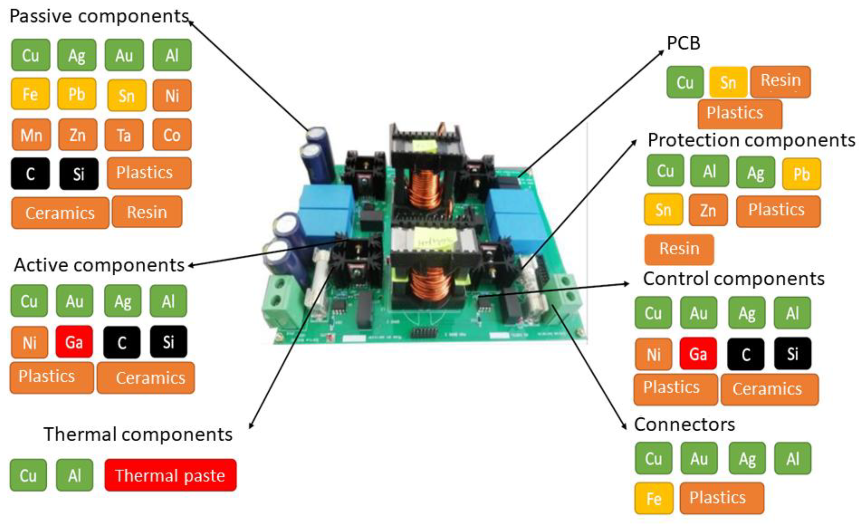
When these converters reach the end of their functional life, optimal management of their recycling faces several difficulties: the difficulty of sorting and then recycling components with heterogeneous metallic (and plastic) compositions. Specific management and recovery issues arise for actors in the Electrical and Electronic Waste (E-waste) treatment industry. Each alloy or metal is not currently being recovered optimally.
Before the converter is broken down into unitary components, one of the difficulties faced by actors upstream of the recovery chain is to diagnose these highly heterogeneous systems when they are defective. The next step is to propose an adapted scheme for maintaining, reusing, repairing or reconditioning these converters specifically.
Thus, knowing the residual value of the components would allow this key actor to diagnose the state of the converter and to optimize its end-of-life scenario.
This research explores reuse of electrical components in the specific context of power electronics and proposes decision-making indicators for end-of-life power converter diagnostics: the residual value. It is divided into three parts:
- The first part presents context, analyzes residual value calculations in other electrical engineering fields related to power electronics, and proposes a residual value formula for electronic components or power converter sub-systems. The parameters needed to calculate the residual value will be detailed in the next two parts with a specific focus on two crucial parameters.
- The second part deals with the residual value parameter of remaining useful life. It proposes a method to monitor online the remaining life of components to inform the residual value formula and make end-of-life decisions.
- The third part deals with the residual value parameter of reusability rate of a component in an electronic set. This part proposes experimental protocols to measure reusability rates through aging evaluations of the extraction process.
The goal of these three parts is to support the decision-making of power electronics component end-of-life scenarios by calculating their residual values at a specific point in their life, by electronics designers, focusing on two key parameters, but leaving room for future research on other key parameters.
2. Definition of the Residual Value in Power Electronics
Residual value is an economic concept widely used by macroeconomists in decision-making. This section presents two application examples in the automotive and battery industries (Section 2.1 and Section 2.2). These examples provide a foundation for defining residual value in power electronics, which is discussed in Section 2.3.
2.1. Residual Value in the Automotive Sector
A used vehicle in France is considered second-hand after 6 months of delivery and over 6,000 km driven. The used car market has dominated the new car market since the 70s. In March 2011, over 510,000 used cars were registered compared to only 257,000 new cars [9]. “Cote Argus,” a valuation reference for used vehicles in the French market, was established in 1927 by Paul Rousseau for the magazine “L’argus.” It serves as a negotiating reference for professionals and is used for trade-ins and private sales. Insurers also use it to estimate repairs or set buyback prices. “Cote Argus” has expanded to cover other vehicles like agricultural vehicles and caravans. Initially, it was a simple average Argus value but has become personalized over time. The value is adjusted based on factors like mileage and extra equipment. There are multiple studies on the depreciation of vehicle value in France and other countries [10,11,12]. According to Boiteux, the most common practice is to depreciate a portion of the initial value each year over a set lifespan. Depreciation is highest in the first years of a vehicle’s life and gradually decreases, as revealed by Argus values for various models since 1927 [13].
Other used car residual value indicators exist in other countries. In NAFTA countries, a manual similar to the Argus called “The Kelley Blue Book” is commonly used by American automakers to evaluate a used vehicle model’s depreciation. This assumes that a vehicle’s value decreases exponentially [14]. This gives the following formula.
where k is a coefficient of depreciation, and are the reparation additional value.
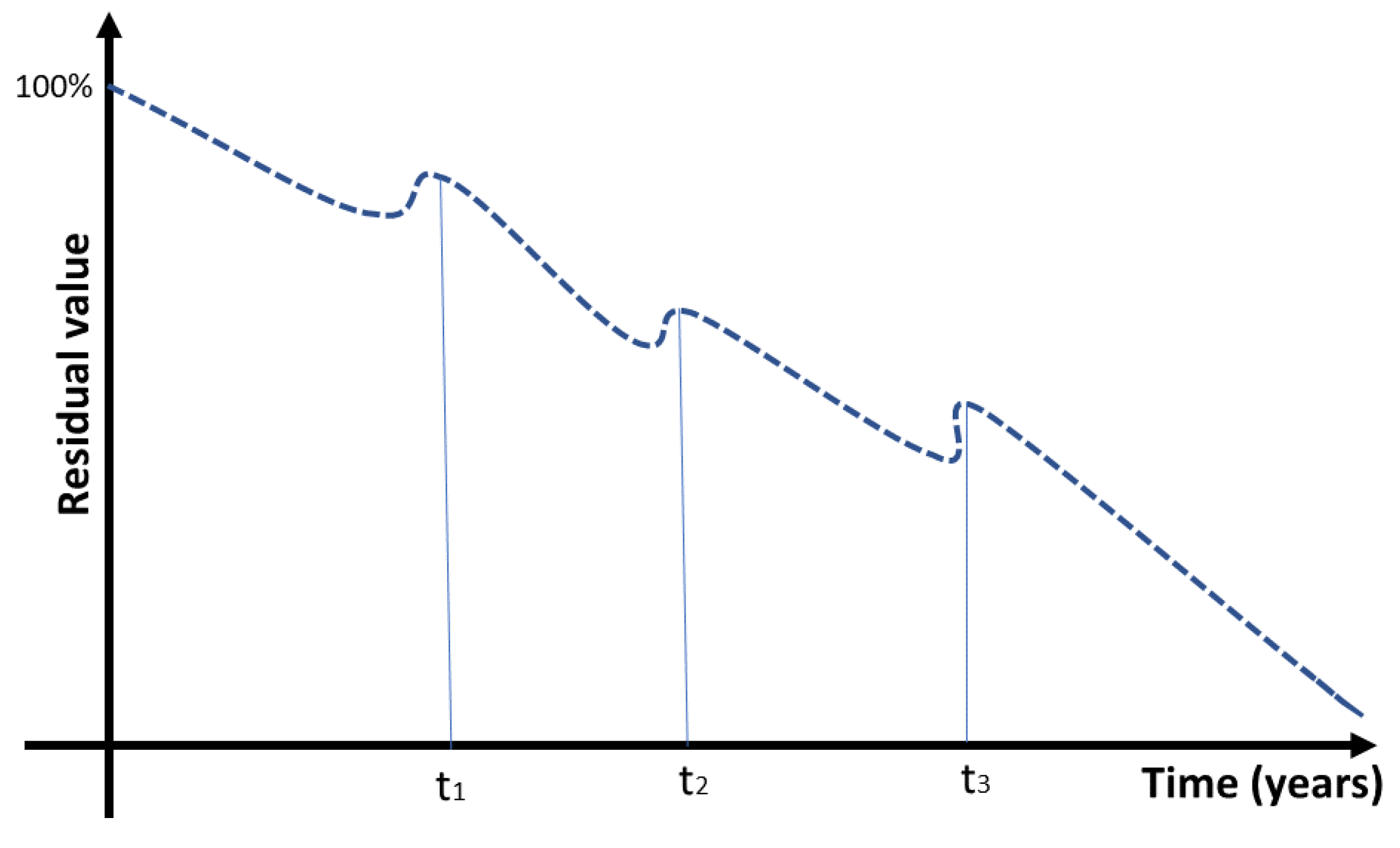
The residual value of a vehicle (except of collectible vehicles ) only decreases after its purchase at t0 until its value is completely lost. In this case, if the owner wants to get rid of the vehicle, it is either scrapped or resold in other unofficial resale circuits.
This depreciation of the value of a vehicle can be schematized according to the formula above as follows in the below figure.
Figure 3.
The evolution of the residual value over time with punctual repair once in a while at t1, t2, t3, ….
Figure 3.
The evolution of the residual value over time with punctual repair once in a while at t1, t2, t3, ….
The used car market is already well established with a structured network of players [15,16]. All actors use value indicators to build trust between buyers and sellers [17]. The market has opened new opportunities for the automotive industry, even leading manufacturers to adapt their business model to the trend of the used car market, offering repair services and replacement parts to maintain a high value for the vehicle.
Emotional factors also play a role in determining a car’s residual value differently from depreciation models. For example, the residual value of the Renault R4 model has remained stable due to its media exposure during sporting events. This allows owners to make heavy changes and repairs without much depreciation.
2.2. Residual Value in Battery Industry
Like all electrical equipment, batteries degrade over time and lose value. Managing end-of-life scenarios is becoming increasingly crucial, as the European Union classifies the metals used in batteries as high-supply risk metals, while installed battery capacity is projected to rise significantly from 200 GWh in 2022 to 1,000 GWh by 2030 [18].
Batteries follow different end-of-life pathways, ranked from the most to the least degrading in terms of functional value: recycling, reuse, reassignment, and remanufacturing. The figure below illustrates these scenarios for an electric vehicle battery.
Figure 4.
Different end-of-life scenarios of Lithium-Ion batteries.
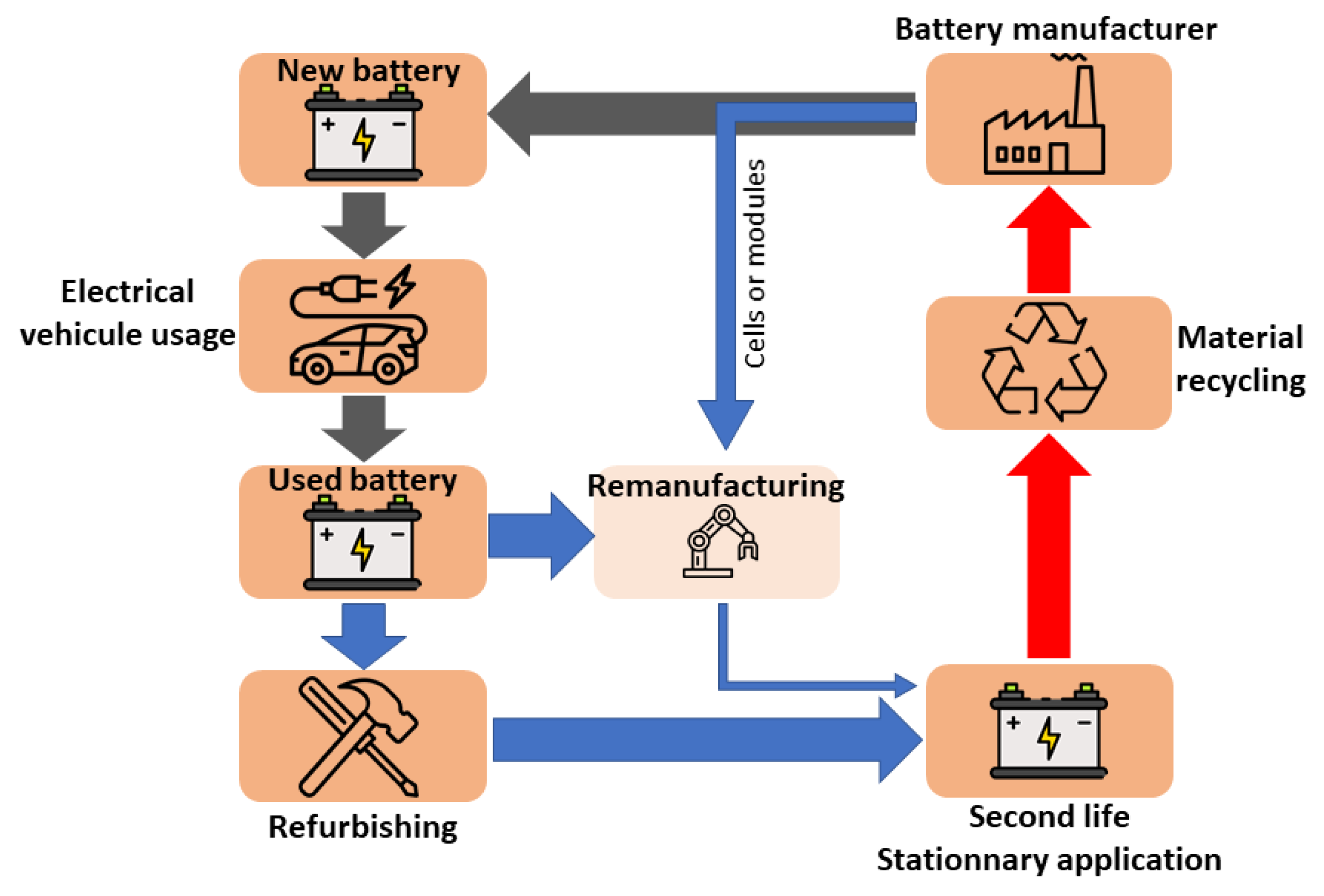
The State of Health (SOH) indicator is a key metric for assessing a battery’s residual value and guiding end-of-life decisions. It is a reference indicator in the used electric vehicle market, helping estimate a vehicle’s overall value. In electric vehicles, batteries are typically guaranteed for 8 years or 160,000 km, provided the SOH remains above 60% [19]. Monitoring SOH is essential for tracking battery aging and optimizing usage.
The dominant end-of-life scenario for lithium-ion batteries is transitioning from mobile to stationary storage once the SOH declines. This shift is driven by the battery’s residual value, which is often more attractive for stationary applications than purchasing a new battery.
The Battery Management System (BMS) typically includes a SOH indicator to facilitate this transition [20]. In line with sustainability goals, the European Union aims to reuse 80% of electric vehicle battery capacity for stationary storage by 2030, relying on accurate health assessments. Batteries can undergo multiple second-life applications before recycling becomes the most viable option.
2.3. Definition of Residual Value in Power Electronics
The value of a converter evolves throughout its life cycle [21]. From the extraction of raw materials needed to manufacture its components, these materials gain functional value through transformation processes such as purification and shaping. These processed materials are then used to produce components with one or more functions, which, when assembled, form a system with added value. This value is determined by the functionality of the converter, the manufacturer’s expertise, and, to a lesser extent, the costs incurred during production, including human resources, energy consumption, environmental impact on air, soil, and water, manufacturing processes, and by-products.
Assembling the components and creating packaging further enhance the converter’s value by introducing multiple and complex functions. Additional value is also generated through the integration of services such as Human-Machine Interfaces (HMI) and monitoring systems. For example, the total manufacturing process, from raw materials to the complete converter, accounts for approximately 50% of the final product’s monetary value in the case of Samsung phone chargers [22]. Logistics and distribution contribute to value as they provide a service to stakeholders throughout the supply chain. Marketing further increases the product’s value by influencing supply and demand, with studies showing that marketing techniques can add up to 20% of the final price, as quantified for Samsung phone chargers [23]. Other factors, such as compliance with safety, EMC, and reliability standards, also increase a converter’s value by allowing it to meet regulatory requirements. Certifications related to eco-design and environmental standards can further enhance its marketability and overall worth [24].
In the early stages of its life, before being put into use, the converter’s residual value only increases until it reaches its selling price. However, in most cases, the economic value of electronic products depreciates over time. Once sold, a converter’s monetary value begins to decline and continues to decrease until it reaches the point of total destruction at the end of its life. Although the monetary value drops, the functional and environmental value may increase due to factors such as upgrades, reuse, and recycling potential. These steps introduce additional costs, including labor, equipment, consumables, storage, and end-of-life processing procedures to extract material resources.
To determine the residual value of power electronics components, the following assumptions are made:
- Residual value is based on usage time and the remaining operational life, following a depreciation model linked to reliability.
- Requalification process costs are additional costs that reduce monetary value but increase functional residual value.
- If the extraction of a component or module from its converter is impossible or would cause damage, its value is considered zero.
- The value can be adjusted by a correction factor during singular events related to socio-economic context and supply difficulties (e.g. geopolitical constraints).
Using these assumptions, the residual value of a power electronics component can be quantified through equation (2).
where k is the socio-economic singularity rectifier, is the initial value of the converter, RLT is the remaining lifetime and is the possibility of a disassembly factor.
3. Monitoring of the Remaining Lifetime
RLT (Remaining Lifetime) is one of the most important parameters in determining the residual value. However, quantifying it in real time remains a significant challenge, as it requires knowledge of all events that have occurred during the converter’s lifetime to accurately estimate it. RLT models are based on reliability theory and the physics of failure. To fully grasp these models, it is essential to first understand the underlying principles of this theory.
3.1. Basics of Physics of Failure
The reliability, denoted R(t), is the ability of a component to perform its function over a given period. It is characterized by the probability that the component operates within specified conditions during a given time.
R(t)=Prob{No failure during [0,t]}
A given component can be in one of two states: a functioning state (where it meets all the specifications outlined in its data sheet) or a failure state (where at least one specification is not met). T is the random variable representing the elapsed time between the commissioning of a component and its first failure. The reliability at time t is the probability that a component does not fail during the period [0, t], defined as:
R(t)=Prob{t<T}
The distribution function of the random variable T is equivalent to the function F(t) (the probability of system failure at time t):
F(t)=Prob{t>T}=1−R(t)
The function f(t) is the probability density function of F(t) and is given by:
The distribution function F(t) and the reliability function R(t) are related to the probability density function f(t) through the following equation
The failure rate, denoted as λ(t), is a characteristic of reliability. The value λ(t)dt represents the conditional probability of a failure occurring within the time interval [t, t+dt], given that no failure occurred during the interval [0, t]. Thus, λ(t) is expressed as:
It appears from this equation that:
To characterize the reliability of components, other metrics are commonly used in industry, such as MTBF (Mean Time Between Failures), which represents the average operational time before failure:
Here, E(T) represents the mathematical expected value of the random variable T.
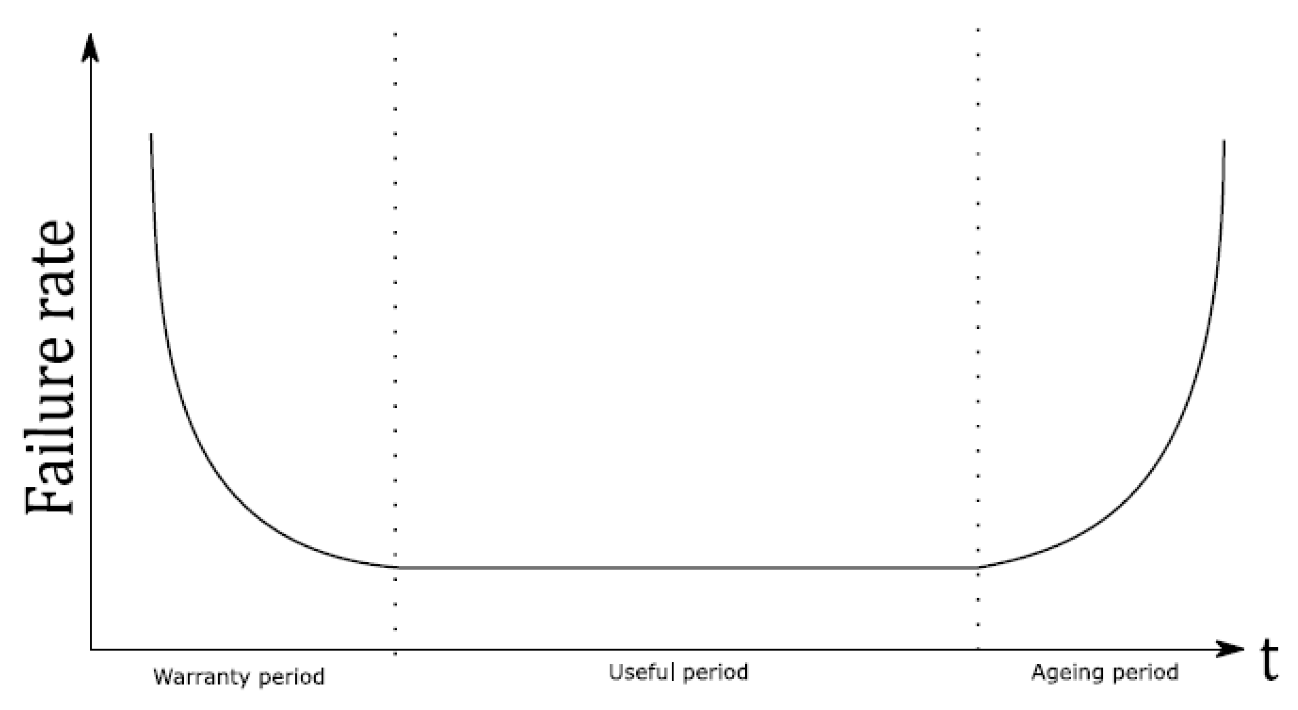
The failure rate of electrical systems, λ, is typically described by the so-called bathtub curve, which shows the evolution of the failure rate over time. This curve highlights three empirical phases in a product’s life cycle:
- ○
- Warranty period: Failures occurring during this period are typically due to manufacturing defects and are not considered in reliability studies. For instance, photovoltaic module manufacturers typically guarantee 5 years against mechanical failures.
- ○
- Useful life period: This represents the majority of a product’s life, where fatigue and wear have not yet significantly impacted the component.
- ○
- End-of-life period: Failure rate increases rapidly during this phase due to wear-out phenomena.
Figure 5.
bathtub curve: Typical Failure Rate Curve over Product Lifetime.
Reliability is a value that requires knowledge of the lifetime distributions, which must account for all failure mechanisms associated with different technologies. Thus, determining R(t) requires knowledge of f(t) and, consequently, λ(t). This can be achieved through aging tests, which help determine the lifetime distribution (random variable T) and, in turn, the reliability metrics. Common distribution laws used in literature [25,26,27] include the exponential, Weibull, and log-normal distributions. To determine the average lifetime of a component, accelerated aging tests must first be conducted to model the aging factors and the lifetime distribution of the component, λ.
Here, λnominal is the failure rate for operation in the component’s nominal operating range, and ΣAF is the sum of the acceleration factors for the component’s aging process.
3.2. Failure Mechanisms
Let’s now take a closer look at the aging process in power electronics, specifically for active power components, for which extensive studies have been conducted. Components age faster when exposed to high temperatures, significant temperature cycles, or mechanical and chemical stresses such as vibrations, corrosion, and humidity. The causes of aging can be classified into four main categories [28]:
Temperature and thermal cycles alone account for about 65% of the aging process. In systems protected against vibrations and humidity, temperature increase becomes the primary cause of failure in power electronics components. Below is an overview of the stresses related to these aging factors.
Thermal and thermoelectric stresses: the acceleration due to temperature in failure mechanisms is modeled by Arrhenius’ law, which is valid for all electronic components. The acceleration factor is multiplicative to the lifetime and reduces it when stresses are high:
where is the activation energy (obtained from accelerated aging tests), is the Boltzmann constant, is the reference level for thermoelectric stress at 20°C and nominal voltage, are the reference temperature and the application temperature and is the applied voltage.
Thermal cycling stresses: These stresses, also called “thermomechanical stresses”, accelerate fatigue mechanisms, modeled by the Norris-Landzberg model [29]. This model accounts for the effect of the duration and frequency of thermal cycles on component reliability, as it activates phenomena like creep (such as the deformation of solder joints). The formula is:
where are experimental parameters, is the temperature range of the thermal cycle, f is the cycle frequency, is the maximum temperature of the cycle.
Humidity-related stresses: Humidity is the ratio between the water vapor pressure in the air and the saturated vapor pressure. The acceleration caused by the combination of humidity and temperature on failure mechanisms is modeled by Peck’s model [30]:
where RH is the relative humidity, a,p are empirical parameters from accelerated aging tests.
Vibration-related stresses (mechanical stresses): the higher the vibration level, the greater the risk of failure in components and electronic boards. Failure mechanisms include cracking (substrates, enclosures), adhesion issues (poor bonding, delamination), and more. The Basquin model [31] is often used for such failure mechanisms:
where Grms is the effective vibration level in the environment.
Now, we have a set of mathematical relationships that express the acceleration factors for aging due to thermal, mechanical, and humidity stresses. The next step is to quantify the different parameters, which is done through accelerated aging studies, in this article FIDES models will be considered for the case study [32].
The FIDES Manual is a guideline for reliability prediction and assessment of electronic components, systems, and assemblies, particularly in the context of high-reliability industries like aerospace, defense, and automotive. It provides a standardized method for evaluating the failure rates of electronic components over time, taking into account environmental conditions, component stress factors, and operational use. The manual is widely used to assess the reliability of complex electronic systems throughout their lifecycle.
3.2. Lifetime Monitoring Methods
Several studies [33,34] have shown that electrolytic capacitors, along with defects related to connectors and PCBs (including soldering), account for 60% of the failure causes in power converters. The remaining portion primarily involves active components (such as semiconductors, their manufacturing techniques, etc.). As a result, health monitoring techniques have been developed in response to these failure sources.
According to [35], significant interest in health state monitoring (HSM) emerged in the 2000s with the measurement of known electrical parameters of components, such as the on-state voltage for switching devices. Subsequently, substantial efforts were made to estimate the internal temperature of components, such as junction temperature for transistors, using gate voltage or threshold voltage measurements [36]. Recently, with the development of acoustic and optical receivers, as well as miniaturization of devices and the advancement of Artificial Intelligence (AI), several non-contact methods have been developed for health monitoring. Table 1 lists the different health state monitoring methods developed in recent years, primarily for active components (MOSFETs, IGBTs, etc.).
Physical and electrical methods: initial Health state management work involved in direct contact with the component’s surface using one or more thermocouples, but few components in real power converter applications include thermocouples due to the bulky and invasive nature of the detection circuit [37,38].
Electrical methods rely on the principle that the properties of materials and semiconductors in components are temperature-dependent during operation. Certain measurable electrical parameters, such as resistance or voltage measurements, can serve as excellent estimators of component temperature. These methods are frequently used for health state monitoring due to their accuracy, low response time, and ease of implementation.
For instance, measuring the variation in electrical resistance Rt of a material can estimate its temperature, provided the variation law of resistivity with temperature is known:
where is the material’s resistance at 0°C and is the material’s temperature/resistance coefficient.
This widely used method is invasive. Furthermore, integrating sensors into components degrades their performance over time [39,40]. Other electrical methods involve correlating the material’s temperature with electrical quantities during operation. For example, the fluctuation in the threshold voltage of a MOSFET can be associated with temperature ranges.
Acoustic methods: acoustic methods have been particularly used to estimate the degradation of transformers and capacitors [41,42]. This is achievable by detecting sound waves emitted by the component. This method eliminates the need for direct contact, unlike voltage sensors, but the physical phenomena and interpretation of acoustic signatures are still under research. Other drawbacks include the cost of the decoding circuit and potential electromagnetic interference. Acoustic methods are typically used for spot checks, not embedded in the system, to characterize components before and after use.
Optical methods: various optical methods have been developed to thermally map power converters using infrared sensors [43,44]. The temperature readings can then be used to feed reliability models. Infrared sensors are inexpensive and non-intrusive, but they only provide the surface temperature of the component, not the temperature at its core. This can result in significant delays and inaccuracies in temperature readings, making them unsuitable for real-time fault detection but useful for long-term remaining life estimations.
Figure 6.
IR image gun on the right and photodiode on the left.
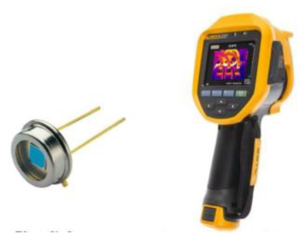
Other optical methods have emerged with the development of Wide-Band-Gap (WBG) devices, enabling higher frequency switching and stimulating research into the electroluminescence of materials such as SiC and GaN [45]. The detection system uses a simple commercial photodiode and decoding circuit to obtain the junction temperature of WBG transistors.
All these methods aim to estimate the temperature within a component while minimizing the added circuit cost, reducing intrusion into the component or system, and maximizing the estimation accuracy and reliability of the entire temperature detection system.
3.3. Temperature-Based Models for Lifetime Monitoring
Power electronics components age more quickly when exposed to higher temperatures, significant temperature cycles, or greater mechanical and chemical stresses such as vibrations, corrosion, or humidity [46]. Temperature and thermal cycles alone account for about two thirds of the aging process. For stationary devices that do not undergo mechanical shocks, thermal cycles are the most impactful. The ability to track and interpret the thermal mission profile of a component in detail could help monitor its aging. If the temperature profile at each moment of the component’s use could be tracked or precisely determined, it would assist in diagnosing the wear state and calculating the potential remaining lifespan of the component.
Power electronic components are heterogeneous in terms of their size, manufacturing processes, material compositions, and assembly techniques. This results in non-homogeneous aging for each component of a given electronic board. To meet the requirements for effective health monitoring of power converters, the health monitoring method proposed here will be based on the following criteria:
- Universal lifespan estimation: the method must be able to evaluate the remaining lifespan of all components.
- Easy integration: the method should be lightweight and not add unnecessary sensors to all components.
- Standardized system approach: the approach should be based on standardized systems that are produced on a large scale.
- State observer creation: a detailed study should allow the creation of an observer that links the thermal parameters of each component to the operational conditions of the converter.
- Embedded observers: the state observer can be embedded in the converter, evaluating the remaining lifespan in real time, avoiding the need to store the mission profile.
- Minimal sensor addition: to minimize costs and maintain reliability, no additional sensors (or very few) should be added to the system.
The proposed method involves three main implementation axes:
- Data collection of temperature: data is collected through thermal imaging and test benches to replicate real operational conditions.
- Building statistical models: the collected thermal data will be used to construct statistical models, combining empirical results and FIDES reliability models.
- Integration into the converter microcontroller: the improved FIDES reliability models are integrated into the converter’s microcontroller to track the remaining lifespan of each component based on the operating conditions of the converter.
According to [47], combining empirical data with optimized statistical models (such as AI models) offers promising methods for health monitoring. This approach addresses multiple challenges, such as considering the interactions between components, ensuring robust tracking, and maintaining non-intrusiveness in monitoring the converter’s overall functioning.
3.4. The Description of the Methodology
3.4.1. Collecting Data
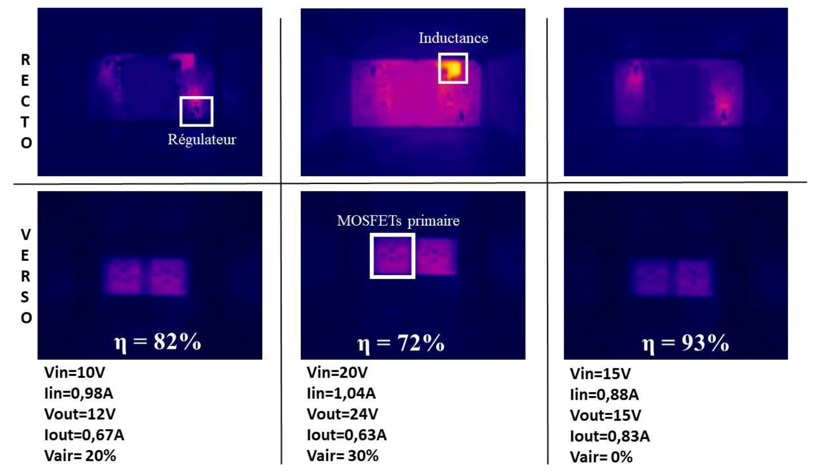
The first goal is to collect Infrared (IR) images at different operating points of the converter to establish a representative database. This database will link the temperature rise of each converter component to its operating point.
Figure 7.
IR photos of a DAB converter operating at different operation points.
3.4.2. Component’s Temperature Models Creation
From the IR images, the temperature rise of each component can be related to the converter’s operating points. A thermal behavior model will be built for each component, and predictive models will be created using MATLAB’s “Regression Learner” tool.
3.4.1. Real-Time Predictive Algorithm
The predictive model created in 3.4.2 will be loaded into the converter’s microprocessor to monitor the real-time temperature of each component, enabling real-time stress tracking and the calculation of accumulated stress over time. This model will be used to estimate the Mean Time Between Failures (MTBF) for a given operating point.
This study employs a lifespan monitoring approach based on the accumulation of aging factors. Previous research has demonstrated that accumulating aging factors to compute the MTBF yields the same results as if the mission profile had been predefined [48]. A commonly used theoretical approach is the Palmgren-Miner rule, a basic stress accumulation model. It assumes that stress accumulates as the ratio between the number of cycles at a given load level and the total number of cycles before failure at that load level.
In our study, each time step corresponds to a cycle transition. The calculated stresses are reintegrated through a time-based rather than cycle-based ratio, following this formula:
Here, the stress at time t accumulates from the stress experienced between [0, t-Δt] and the new stress applied between [t, t+Δt]. This results in a weighted average of past and present stresses.
However, this necessitates an adjustment to the FIDES thermal cycling stress model for electronic components. For instance, the thermal cycling aging model for an inductor is modified as follows:
where N=1, since the exact number of cycles at a given operating point is unknown, is the sampling time and is the temperature difference between two successive cycles.
Figure 8.
Schematic of the thermal stress accumulation on the left and on the right the MTBF tracking with time.
Figure 8.
Schematic of the thermal stress accumulation on the left and on the right the MTBF tracking with time.
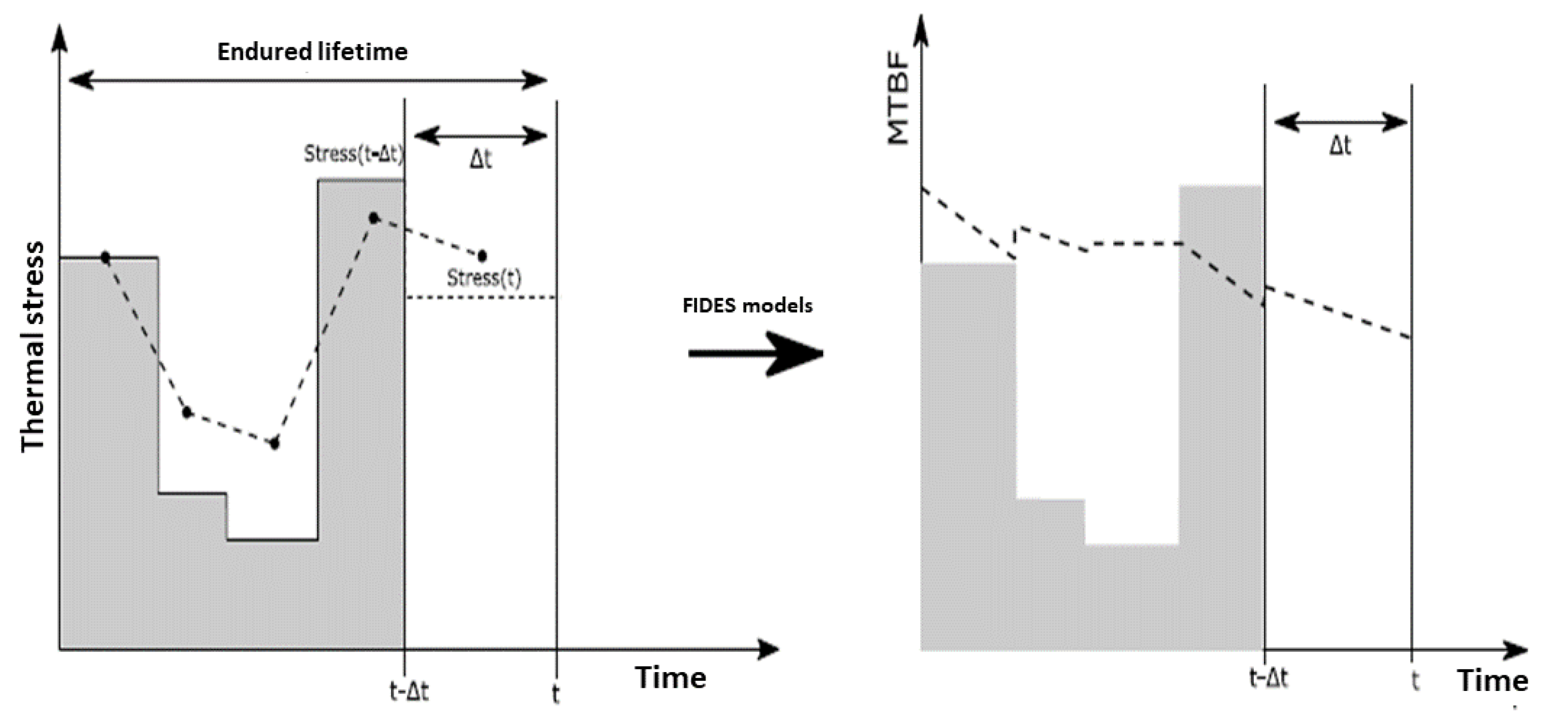
The figure above illustrates the step-by-step computation of accumulated thermal stress and its integration into the MTBF calculation. The left graph shows how cumulative stress is tracked over time, while the right graph demonstrates how this accumulated stress updates the MTBF to reflect the real operating conditions of the component.
For a more detailed explanation of the lifetime monitoring algorithm, refer to [49].
4. The Impact of Disassembly on the Remaining Lifetime
4.1. Disassembly Methods
To extract a component or a subassembly from a printed circuit board (PCB), it is necessary to melt the solder to detach the component pins from the PCB pads. Various assembly techniques can also be reversed for disassembly, each with its own advantages and disadvantages.

Table 2.
PCB components disassembly methods.
| Methods | Tools | Advantages | Disadvantages |
|---|---|---|---|
| Surface scraping | Pruning shears | Not polluting High volumes |
- The host PCB is destroyed - Requires cleaning - The component is still attached to a part of the PCB |
| Manually | Soldering iron + solder braid | Easy to implement | - Requires manual labor - Slow and inefficient for small components |
| Hot air | Hot air gun | Not polluting and fast | - Low precision control - Poor energy efficiency - Component temperature rise |
| Infrared ovens | Radiator + vibration | Not polluting and fast | Thermal damaging |
| Soldering ovens | Reflow oven + vibration | - Fast for assembly line processing - Efficient for large volumes of defective PCBs |
Non-targeted heat |
| Chemical | Epoxy treatment solutions or tin alloy dissolution solutions. | - Directly targets the solder - Low labor requirement |
- Polluting - Risk of damaging the component |
| Automatic | Robotic arm | Targeted heat | - Low throughput - Expensive |
Among these methods, the reflow oven is the most widely used for assembling Surface-Mount Components (SMCs) and is already present in manufacturing facilities. However, modifying the oven is required for automated disassembly, ensuring that components can be efficiently extracted without damage.
The reflow soldering process consists of four distinct phases, each with specific temperature settings and holding times. The temperature profile depends on various factors, such as the component type, solder composition, and PCB configuration.
- Preheating Phase: the PCB temperature gradually rises from ambient temperature to ~150°C, with a controlled ramp-up rate (0.75°C to 2°C per second). This step prevents thermal shock and eliminates residual chemicals.
- Soaking Phase: temperature stabilization ensures uniform heating across all components. During this phase, the flux in the solder paste activates, removing oxides from component leads and PCB pads to enhance electrical contact.
- Reflow Phase: solder particles melt and form metallurgical bonds between component pins and copper traces. The peak temperature must be high enough to liquefy the solder while avoiding component degradation.
- Cooling Phase: the PCB naturally cools using a fan, allowing the solder to solidify. This phase is critical for assembly but less relevant for disassembly, where precise cooling control is unnecessary.
Reflow ovens can have multiple heating zones, each with specific temperature settings, or single-zone configurations, where thermal resistance is adjusted to achieve the different phases. Multi-zone ovens are most commonly used for mass production as they allow for high-throughput processing.
For assembling components on PCBs, two major categories of solder are used in PCB assembly, each with distinct properties affecting the reflow process:
Table 3.
Type of solders in power electronics.
| Type of Solder | Characteristics |
|---|---|
| Lead-based solder | Lead-containing solder alloys melt at relatively low temperatures (~180°C). However, due to environmental concerns, lead was banned after the 2011 European RoHS directive. These alloys typically contain 60% tin and 40% lead (e.g. Sn62Pb36Ag2 or Sn63Pb37). |
| Lead free solder | These alloys comply with the RoHS directive and are typically composed of 90% tin. They require higher melting temperatures (up to 270°C) and are more expensive. |
The choice between these alloys depends on thermal conductivity, mechanical strength, activation energy, and reflow temperature, as shown in Figure 9. The smaller the solder particle size, the more precise the deposition but the higher the cost.
Additionally to solder, flux is essential in reflow soldering as it prevents oxidation and improves wetting between the solder and component leads. There are three main types of flux:
- Rosin-based (R): requires minimal cleaning, common in consumer electronics.
- Inorganic acid flux (NR): leaves minimal residue, used in industrial applications.
- Water-Soluble (WS): easily washable, environmentally preferred (less polluting) but requires additional cleaning steps.
Flux selection significantly impacts reflow efficiency, oxidation prevention, and residue cleanup. Figure 10 provides a decision chart for flux types based on reflow duration and cleaning needs.
4.2. The Impact of Disassembly on SMD Electrolytic Capacitors
4.2.1. Aging Mechanisms of Capacitors
Electrolytic capacitors are widely used in power electronics due to their high capacitance values, compact size, and cost effectiveness. They serve as local energy storage components, helping to filter electrical signals and compensate for brief power interruptions. There are two main types: aluminum and tantalum capacitors, with aluminum electrolytic capacitors being the most common, primarily used for filtering and energy storage.
These capacitors consist of:
- A hermetically sealed aluminum casing to prevent electrolyte leakage.
- Stacked aluminum foils and insulating layers impregnated with electrolytes.
- A rubber sealing disc and a cover to maintain integrity.
- Two terminals: one connecting the anode foils and the other the cathode foils.
Much aluminum electrolytic capacitors, particularly surface-mounted (SMD) versions, are designed to withstand the reflow soldering process. A safety valve is often included to release excess pressure caused by electrolyte evaporation.
Electrolytic capacitors are commonly represented as a capacitance CCC in series with an Equivalent Series Resistance (ESR). Some models also include an Equivalent Series Inductance (ESL), but for low-frequency applications, ESL is typically neglected. Another key parameter is Equivalent Parallel Resistance (EPR), which accounts for the leakage of currents. As capacitors age, CCC, ESR, and EPR degrade, impacting performance and indicating the component’s health.
Capacitor degradation is mainly due to:
- Breakdown of the oxide dielectric layer.
- Electrolyte depletion and changes in its properties.
- Leakage of electrolytes through seals or self-regeneration of the oxide layer.
During high-temperature processes such as reflow soldering, exceeding the electrolyte’s boiling point can cause irreversible damage. The primary indicators of aging are
- Increase in ESR – indicating higher internal resistance.
- Decrease in Capacitance – resulting from dielectric deterioration.
Industry standards define a capacitor’s end-of-life as an ESR increase of 100% and a capacitance decrease of 20%.
4.2.2. Aging Experimental Setup
A study was conducted using 10 Panasonic ZA-series SMD capacitors. Key specifications included:
Table 4.
The characteristic of the studied capacitor.
| Parameter | Value |
|---|---|
| Capacity | 33 μF |
| Maximum temperature | 105°C |
| Nominal voltage | 7 V |
| ESR max (120Hz,20°C) | 300mOhm |
| Theoretical MTBF | 5 years |
The capacitors underwent ten reflow cycles at 270°C (30s peak temperature) and 100°C (120s soak time). ESR and capacitance were measured before and after each cycle using an Agilent impedance meter.
Figure 11.
experimental setup for disassembly characterization.
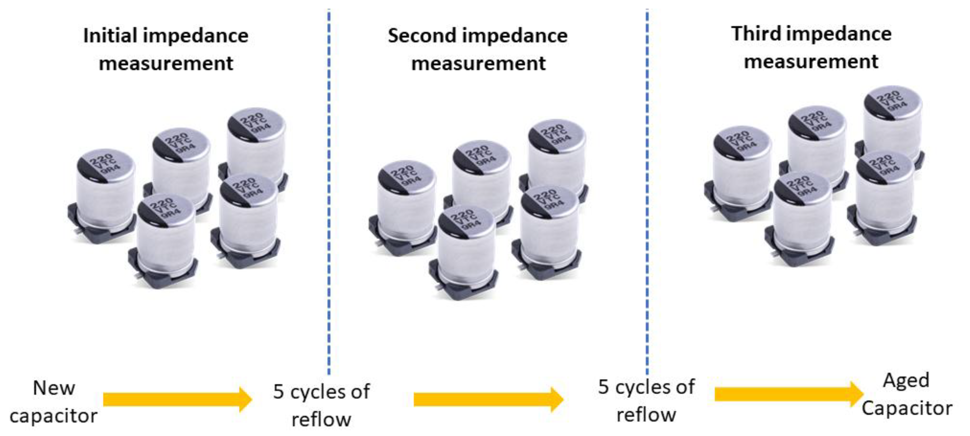
ESR increased by 25% after five reflow cycles, confirming degradation beyond measurement error.
Figure 12.
The evolution of the capacity and ERS with reflow oven cycling.
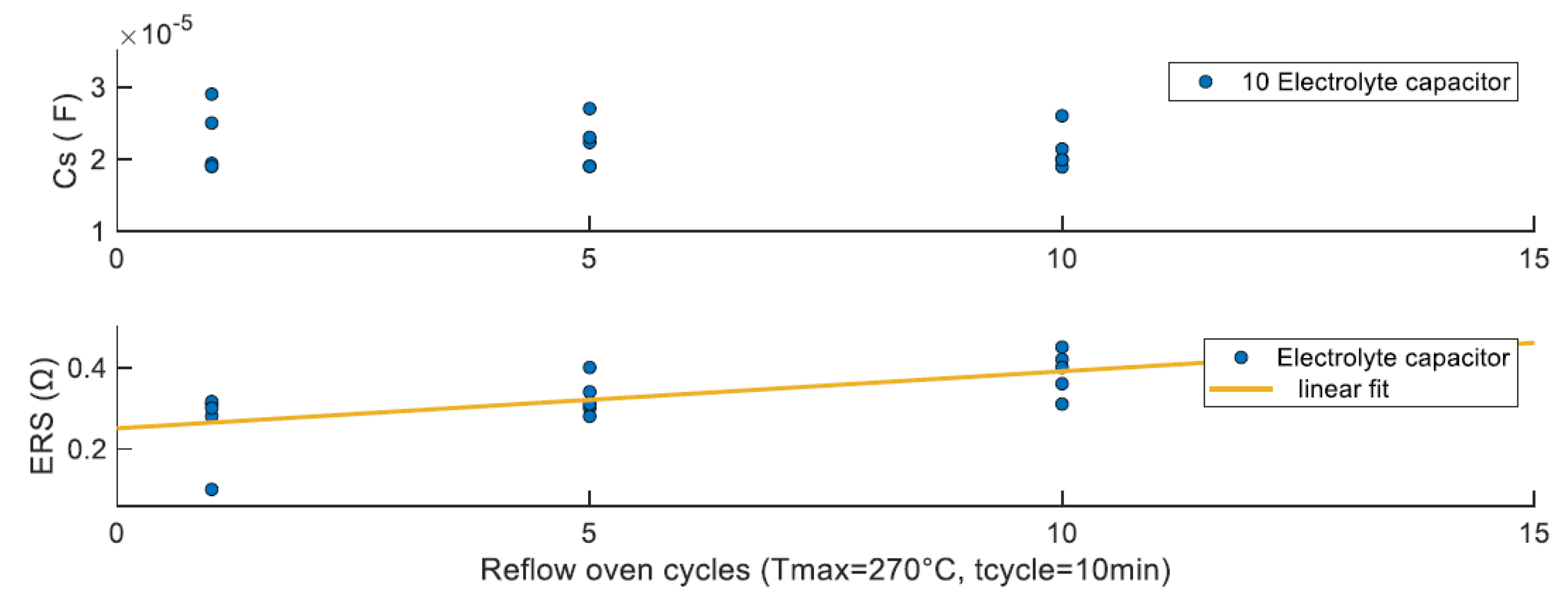
A linear ESR growth model was observed:
Capacitance showed minor reduction, insufficient to conclude significant dielectric degradation.
Reflow soldering significantly impacts electrolytic capacitor aging, particularly by increasing ESR. Given their susceptibility to failure, these components are rarely reused and are typically recycled. Future research is exploring remanufacturing methods for large electrolytic capacitors.
4.3. The Impact of Disassembly on a SMD HF Planar Transformer
The high-frequency (HF) transformer is one of the most durable and resilient components in power electronics circuits. It primarily converts an AC voltage to another AC voltage of the same frequency but different amplitude, adapting it to specific applications. Additionally, it provides galvanic isolation, commonly between the power stage and the control stage in a converter.
The studied transformer is a Coilcraft planar transformer (model “120W PoE SMT PLANAR”). It consists of multiple magnetically coupled winding around a ferrite core. This transformer plays a crucial role in the standardized power conversion cells used in the converter network approach developed at G2ELab, supporting both DC/DC and DC/AC applications.
4.3.1. Aging Mechanisms and Experimental Results
Planar transformers experience three primary types of degradation:
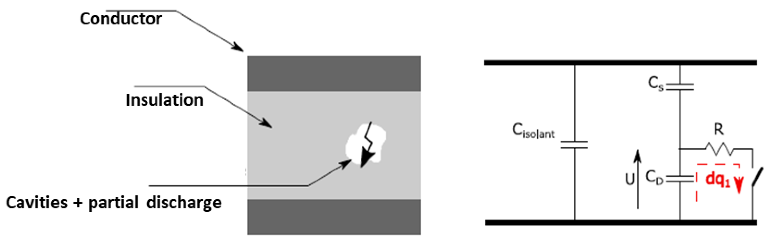
- Insulation Breakdown: Insulation materials (e.g. epoxy resin, PVC, mica) degrade over time due to temperature stress, leading to cracks and reduced dielectric properties. Partial discharge tests, primary-secondary capacitance, and parallel resistance measurements can indicate insulation wear.
- Magnetic Core Aging: The ferrite core is thermally stable, but the adhesive bonding between core sections deteriorates over time, causing misalignment. This misalignment alters the magnetizing inductance, which serves as an indicator of core degradation.
- b>Winding and PCB Deterioration: Copper winding insulation weakens, and PCB deformations due to heat lead to microcracks. Oxidation of exposed copper and solder joint movement affect transformer structure and leakage inductance. Resonance frequency changes can indicate dielectric aging of windings.
Figure 13.
Partial discharge creation of the insulation material of a transformer.
4.3.2. Experimental Set Up
To evaluate the impact of transformer extraction processes on residual value and component characteristics, a dedicated study was conducted. Transformers were subjected to multiple thermal cycles in reflow ovens, followed by measurements of key performance indicators at different stages. Although reusing the same device multiple times is not planned, the aging protocol aims to identify trends that can serve as indicators of component residual value.
This experimental method does not account for aging due to usage or storage, which is typically covered by other studies or manufacturer specifications. However, if components operate within their nominal range during their lifespan, the effects of both aging phases could be combined.
Preliminary tests were performed on a sample transformer to calibrate the experimental limits. These tests determined that 20 thermal reflow cycles were necessary to identify clear trends. The main phase of the experiment involved 10 transformers, with two extracted at each stage for dielectric strength evaluation through partial discharge measurements.
The figures in the article [50] illustrates the experimental process: after every 10 reflow cycles, impedance meter measurements and partial discharge tests were conducted. The key electrical parameters assessed included:
- Magnetizing inductance (measured with an impedance meter with an open-circuited secondary)
- Leakage inductance (measured with a short-circuited secondary)
- Primary-to-secondary capacitance (measured with both windings short-circuited)
- Partial discharge inception voltage, which indicates insulation degradation under high voltage
Partial discharge measurements follow IEC 60270 standards and were conducted using the ICMsys8. The test setup, including a low-noise high-voltage source, a RPA1 preamplifier, and a CC20B conditioning module, ensures precise detection of discharge signals. These tests were performed on the extracted transformers after each reflow cycle to track insulation degradation.
The same oven and measurement equipment used for electrolytic capacitors in the previous section were employed here, ensuring consistent measurement accuracy. The partial discharge test exhibited minimal errors (a few volts on hundreds of volts applied).
After 20 reflow cycles, no transformer exhibited irreversible failure. The only reduction in sample size occurred due to transformers removed after partial discharge tests as a precaution.
Key Observations:
- Magnetizing inductance decreased by ~20% after 20 cycles.
- Leakage inductance and primary-secondary capacitance showed no significant trend due to initial component variability and measurement noise.
- A partial discharge inception voltage dropped by ~20%, indicating insulation degradation.
Despite these variations, the standard deviations remained within acceptable limits (typical tolerances for magnetic component parameters range from 3% to 30%, depending on the manufacturer).
Literature suggests that high temperatures impact magnetic materials, causing increased losses over time. Iron-based amorphous materials, iron powders, and ferrites show progressive but irreversible deterioration months after exposure to elevated temperatures. Similarly, thermal cycling affects insulation behavior, leading to drying, cracking, and expansion.
Due to high initial parameter variability, absolute value thresholds are unreliable for degradation assessment.
4.3.3. Link with the Remaining Lifetime
The main constraints affecting the aging of planar transformers are temperature, the voltage applied to their terminals, and the ripple current passing through them. In the case of a disassembly process, only temperature influences the transformer’s lifespan. In the literature, a transformer is considered worn out if its dielectric withstand voltage decreases by more than 20% from its initial value.
Aging tests for high-frequency dry-type transformers refer to the IEC 60076-12 standard. Transformers are subjected either to current variations or ambient temperature variations, and throughout these tests, their characteristics are monitored. Additionally, aging tests related to disassembly processes must be considered.
Several manufacturers in the literature propose a simplified formulation of transformer lifespan as a function of environmental constraints:
where is the lifespan under extreme operating conditions (maximum Curie temperature and maximum current ripple), as specified in the transformer’s data sheet. represents the lifespan under a given usage profile in hours, and is the aging multiplication factor due to temperature.
For aging tests related to disassembly processes, only temperature is considered in the calculation of the remaining lifespan. The model then becomes:
To complete the aging model for disassembly processes, it is necessary to determine the activation energy Ea. A simplified formulation exists for qualitative accelerated aging cycle tests:
To compute this value, two accelerated aging tests must be performed on the transformer under different temperature cycling conditions. It is worth noting that the activation energy for normal aging of a planar transformer during use is typically within the range Ea∈[0.9eV,2eV].
Similarly, the same methodology can be applied to capacitor aging results. The main factors influencing capacitor degradation include temperature, applied voltage, and ripple current. Under disassembly conditions, temperature remains the dominant factor affecting lifespan. By adapting the existing aging models, capacitor aging can be characterized using equivalent parameters such as activation energy and lifetime factor adjustments. Accelerated aging tests with different temperature cycles can be conducted to determine activation energy, providing a predictive model for capacitor degradation under various conditions.
6. Conclusion and Discussion
Considering the urge to design circular power electronics, this paper explored the way to keep residual value over time. Over its lifetime, a power converter degrades, with each component aging at different rates. As a result, various subsystems have different residual values when the entire converter fails. Assessing the residual value of each component is crucial to determining whether they can be salvaged and reused instead of being discarded. The residual value of an electronic component represents its remaining functionality after a certain period of use under specific conditions. It reflects the component’s ability to continue performing its intended tasks and is influenced by aging, electrical, and material property degradation. However, in cases of supply shortages, this value can increase.
Residual value assessment should not be limited to cost estimation. Several factors influence a component’s functional value, including:
- Reuse Rate: an empirical value based on repair experiments, indicating how many times a component can be successfully reused. This factor integrates functional complexity into the assessment.
- Environmental Impact & Reuse Costs: a theoretical indicator combining disassembly tools, time, energy consumption, and environmental footprint.
- Remaining Lifetime (RLT): a component retains its value if its remaining lifespan is significant.
This residual value should be determined during the diagnostic phase, immediately after the last use, helping manufacturers decide whether refurbishment is viable. Unlike economic value, the functional residual value is a decision-support indicator for component health classification. The economic value can be derived by factoring in refurbishment costs and associated margins.
Existing component health monitoring methods for safety purposes rely on either model-based or sensor-based approaches. This research proposes a hybrid method that monitors residual value by tracking the remaining lifespan at the component and subsystem levels. The approach combines:
- FIDES failure models, an empirical reliability calculation framework for electronic components and systems.
- Experimental methods using infrared (IR) thermal imaging to capture component degradation.
The combination of these methods enhances theoretical model accuracy, allowing dynamic adjustment of a component’s functional residual value. The goal is to improve expertise in power electronics diagnostics and contribute to circular economy strategies for sustainable electronics use.
Key Research Contributions:
- Residual Value Function Modeling: a generic function for residual value estimation is introduced, incorporating parameters like Mean Time Between Failures (MTBF). Inspired by methodologies in the automotive sector, this quantification aids end-of-use decision-making during diagnostic phases.
- Reuse Rate Estimation for Passive Components: a method for estimating the reuse rate of passive components is proposed. Accelerated aging tests, particularly reflow oven cycling, provides degradation trends. Results suggest that robust components, like transformers, may outlast their datasheet specifications, whereas fragile components, such as electrolytic capacitors, degrade rapidly, making their reuse challenging.
-
Real-Time MTBF Estimation for Power Converters: a real-time MTBF estimation method is developed for standard power converters. This involves:
- Pre-use temperature data collection using thermal cameras and test benches.
- Statistical modeling based on collected data, integrated with FIDES reliability models and empirical results.
- Embedded implementation in the converter’s microcontroller for continuous health monitoring, allowing real-time tracking of each component’s remaining lifespan.
These studies contribute to improved diagnostics for power converter components, paving the way for their reuse in an industrial context. By integrating real-time monitoring and advanced reliability modeling, this research moves toward a practical implementation of component reuse in circular electronics.
Author Contributions
Conceptualization, B.R., Y.L.,M.R. and J-C.C.; methodology, B.R.; software, B.R.; validation, B.R., Y.L.,M.R. and J-C.C.; formal analysis, B.R., Y.L.,M.R. and J-C.C.; investigation, B.R.; data curation, B.R.; writing—original draft preparation, B.R.; writing—review and editing, B.R., Y.L.,M.R. and J-C.C. All authors have read and agreed to the published version of the manuscript.
Funding
This research was founded by French public research funding, and received no external or private funding.
Acknowledgments
The experiments were performed in G2Elab and CEDMS in Grenoble, France.
Conflicts of Interest
The authors declare no conflicts of interest. The funders had no role in the design of the study; in the collection, analyses, or interpretation of data; in the writing of the manuscript; or in the decision to publish the results.
References
- STEFFEN: Will, SANDERSON, Regina Angelina, TYSON, Peter D., et al. Global change and the earth system: a planet under pressure. Springer Science & Business Media. 2006.
- DIEDEREN, A. M. Metal minerals scarcity: A call for managed austerity and the elements of hope. TNO Defence, Security and Safety, 2009, p. 2.
- Critical Raw Materials Resilience: Charting a path towards greater security and sustainability document date : 02/09/2020 – Created by GROW.R.2.DIR – Publication date n/a Last update 03/09/2020.
- Rockström, J.; Steffen, W.; Noone, K.; Persson, Å.; Chapin, F.S., III; Lambin, E.; Lenton, T.M.; Scheffer, M.; Folke, C.; Schellnhuber, H.J.; et al. Planetary boundaries: exploring the safe operating space for humanity. Ecol. Soc. 2009, 14, 32. [Google Scholar] [CrossRef]
- VENN, Fiona. The oil crisis. Routledge. 2016.
- LENTON, Timothy M., ROCKSTRÖM, Johan, GAFFNEY, Owen, et al. Climate tipping points—too risky to bet against. 2019.
- SACHS, Jeffrey, KROLL, Christian, LAFORTUNE, Guillame, et al. Sustainable development report 2022. Cambridge University Press. 2022.
- S&P Global. (2022). The Future of Copper: Will the Looming Supply Gap Short-circuit the Energy Transition? IHS Markit. Retrieved from https://cdn.ihsmarkit.com/www/pdf/1022/The-Future-of-Copper_Full-Report_SPGlobal.pdf.
- Le marché de l’automobile d’occasion rembraye [archive] « Copie archivée » (version du 22 avril 2012 sur l’Internet Archive) - Emmanuel Egloff, Le Figaro, 21 avril 2011.
- Gupta, S.M.; Güngör, A.; Govindan, K.; Özceylan, E.; Kalaycı, C.B.; Piplani, R. Responsible & sustainable manufacturing. International Journal of Production Research 2020, 58, 7181–7182. [Google Scholar]
- Feltham, G.A.; Ohlson, J.A. Uncertainty Resolution and the Theory of Depreciation Measurement. J. Account. Res. 1996, 34, 209. [Google Scholar] [CrossRef]
- Wan, J.; Qiu, Q. Depreciation Rate by Industrial Sector and Profit after Tax in China. Chin. Econ. 2021, 55, 111–128. [Google Scholar] [CrossRef]
- Boiteux, M. L’amortissement dépréciation des automobiles. Revue de statistique appliquée 1956, 4, 57–73. [Google Scholar]
- Cote Argus RENAULT Kangoo, la valeur de référence - L’argus (largus.fr).
- Shafiulla, B. Marketing Strategies of Car Makers in the Pre-Owned Car Market in India. Indian Journal of Marketing 2012, 42, 8–16. [Google Scholar]
- Prado, S.M.; et al. The European used-car market at a glance: Hedonic resale price valuation in automotive leasing industry. Economics Bulletin 2009, 29, 2086–2099. [Google Scholar]
- SENTENAC-CHEMIN, Elodie et LANTZ, Frédéric. ANALYSE DES TENDANCES ETDES RUPTURES SURLE MARCHE AUTOMOBILE FRANCAIS.
- Second-life EV batteries: The newest value pool in energy storage by Hauke Engel, Patrick Hertzke, and Giulia Siccard.
- CORON, Eddy. Diagnostic d’état de santé des batteries au lithium utilisées dans les véhicules électriques et destinées à des applications en seconde vie. 2021. Thèse de doctorat. Université Grenoble Alpes [2020-....].
- Second Life-Batteries As Flexible Storage For Renewables Energies.
- https://op.europa.eu/en/publication-detail/-/publication/c6199b83-a368-4853-8bed-bc678404221e.
- Montoya-Bedoya, S.; Sabogal-Moncada, L.A.; Garcia-Tamayo, E.; Martínez-Tejada, H.V. A circular economy of electrochemical energy storage systems: Critical review of SOH/RUL estimation methods for second-life batteries. Green Energy and Environment 2020, 10. [Google Scholar] [CrossRef]
- Serzhena, T. The circular economy on South Korea. The case of Samsung. Hungarian Agricultural Engineering 2019, 36, 75–80. [Google Scholar] [CrossRef]
- Davis, N.T.; Hoomaan, E.; Agrawal, A.K.; Sanayei, M.; Jalinoos, F. Foundation reuse in accelerated bridge construction. Journal of Bridge Engineering 2019, 24, 05019010. [Google Scholar] [CrossRef]
- Hawkes, A.G. A Bivariate Exponential Distribution with Applications to Reliability. J. R. Stat. Soc. Ser. B Statistical Methodol. 1972, 34, 129–131. [Google Scholar] [CrossRef]
- Mccool, J.I. Using the Weibull Distribution: Reliability, Modeling, and Inference; John Wiley & Sons: Hoboken, NJ, USA, 2012. [Google Scholar]
- Balasooriya, U.; Balakrishnan, N. Reliability sampling plans for lognormal distribution, based on progressively-censored samples. IEEE Trans. Reliab. 2000, 49, 199–203. [Google Scholar] [CrossRef]
- Chen, Z.; Guerrero, J.M.; Blaabjerg, F. A review of the state of the art of power electronics for wind turbines. IEEE Trans. Power Electron. 2009, 24, 1859–1875. [Google Scholar] [CrossRef]
- Lall, P.; Shirgaokar, A.; Arunachalam, D. Norris–Landzberg Acceleration Factors and Goldmann Constants for SAC305 Lead-Free Electronics. J. Electron. Packag. 2012, 134, 031008. [Google Scholar] [CrossRef]
- Peck, D.S. Comprehensive model for humidity testing correlation. In : 24th International Reliability Physics Symposium. IEEE, 1986. p. 44-50.
- D'Antuono, P. An analytical relation between the Weibull and Basquin laws for smooth and notched specimens and application to constant amplitude fatigue. Fatigue Fract. Eng. Mater. Struct. 2019, 43, 991–1004. [Google Scholar] [CrossRef]
- https://www.fides-reliability.org/Li, D.; Li, X. Study of degradation in switching mode power supply based on the theory of PoF. In Proceedings of the International Conference Computing Science and Service Systems, Nanjing, China, 11–13 August 2012; pp. 1976–1980.
- Jiang, N.; Zhang, L.; Liu, Z.Q.; Sun, L.; Long, W.M.; He, P.; Xiong, M.Y.; Zhao, M. Reliability issues of lead-free solder joints in electronic devices. Sci. Technol. Adv. Mater. 2019, 20, 876–901. [Google Scholar] [CrossRef]
- Susinni, G.; Rizzo, S.A.; Iannuzzo, F. Two Decades of Condition Monitoring Methods for Power Devices. Electronics 2021, 10, 683. [Google Scholar] [CrossRef]
- AGARWAL, Mridul, PAUL, Bipul C., ZHANG, Ming, et al. Circuit failure prediction and its application to transistor aging. In : 25th IEEE VLSI Test Symposium (VTS’07). IEEE, 2007. p. 277-286.
- Parsley, M. The use of thermochromics liquid crystals in research applications, thermal mapping and non-destructive testing.
- Brekel, W.; Duetemeyer, T.; Puk, G.; Schilling, O. Time Resolved in situ Tvj Measurements of 6.5 kV IGBTs during Inverter Operation. In Proceedings of the PCIM Europe 2009: International Exhibition & Conference for Power Electronics Intelligent Motion Power Quality, Nurember, Germany, 12–14 May 2009. [Google Scholar]
- Motto, E.R.; Donlon, J.F. IGBT module with user accessible on-chip current and temperature sensors. In Proceedings of the Twenty-Seventh Annual IEEE Applied Power Electronics Conference and Exposition (APEC), Orlando, FL, USA, 5–9 February 2012; pp. 176–181. [Google Scholar]
- Ka, I.; Avenas, Y.; Dupont, L.; Vafaei, R.; Thollin, B.; Crebier, J.C.; Petit, M. Instrumented chip dedicated to semiconductor temperature measurements in power electronic converters. In Proceedings of the IEEE Energy Conversion Congress and Exposition (ECCE), Milwaukee, WI, USA, 18–22 September 2016; pp. 1–8. [Google Scholar]
- Jasperneite, J.; Sauter, T.; Wollschlaeger, M. Why We Need Automation Models: Handling Complexity in Industry 4.0 and the Internet of Things. IEEE Ind. Electron. Mag. 2020, 14, 29–40. [Google Scholar] [CrossRef]
- Cheraghi, M.; Karimi, M.; Booin, M.B. An investigation on acoustic noise emitted by induction motors due to magnetic sources. In Proceedings of the 9th Annual Power Electronics, Drives Systems and Technologies Conference (PEDSTC), Tehran, Iran, 13–15 February 2018; pp. 104–109. [Google Scholar]
- Luo, H.; Wang, X.; Zhu, C.; Li, W.; He, X. Investigation and emulation of junction temperature for high-power IGBT modules considering grid codes. IEEE J. Emerg. Sel. Top. Power Electron. 2018, 6, 930–940. [Google Scholar] [CrossRef]
- Hunger, T.; Schilling, O. Numerical investigation on thermal crosstalk of silicon dies in high voltage IGBT modules. In Proceedings of the PCIM International Exhibition & Conference for Power Electronics, Intelligent Motion, Power Quality, Nuremberg, Germany, 27–29 May 2008. [Google Scholar]
- Ceccarelli, L.; Luo, H.; Iannuzzo, F. Investigating SiC MOSFET body diode’s light emission as temperature-sensitive electrical parameter. Microelectron. Reliab. 2018, 88–90, 627–630. [Google Scholar] [CrossRef]
- Fischer, K.; Stalin, T.; Ramberg, H.; Wenske, J.; Wetter, G.; Karlsson, R.; Thiringer, T. Field-Experience Based Root-Cause Analysis of Power-Converter Failure in Wind Turbines. IEEE Trans. Power Electron. 2014, 30, 2481–2492. [Google Scholar] [CrossRef]
- Peyghami, S.; Palensky, P.; Blaabjerg, F. An Overview on the Reliability of Modern Power Electronic Based Power Systems. IEEE Open J. Power Electron. 2020, 1, 34–50. [Google Scholar] [CrossRef]
- Kauzlarich, J.J. The Palmgren-Miner Rule Derived; Tribology Series; Elsevier: Amsterdam, The Netherlands, 1989; pp. 175–179. [Google Scholar]
- Rahmani, B.; Rio, M.; Lembeye, Y.; Crebier, J.-C. Design for reuse: Residual value monitoring of power electronics’ components. Procedia CIRP 2022, 109, 140–145. [Google Scholar] [CrossRef]
- Rahmani, B.; Lembeye, Y.; Crebier, J.-C.; Rio, M. Analysis of passive power components reuse. In PCIM Europe Digital Days 2021: International Exhibition and Conference for Power Electronics, Intelligent Motion, Renewable Energy and Energy Management. VDE Verlag. 2021; pp. 1–8.
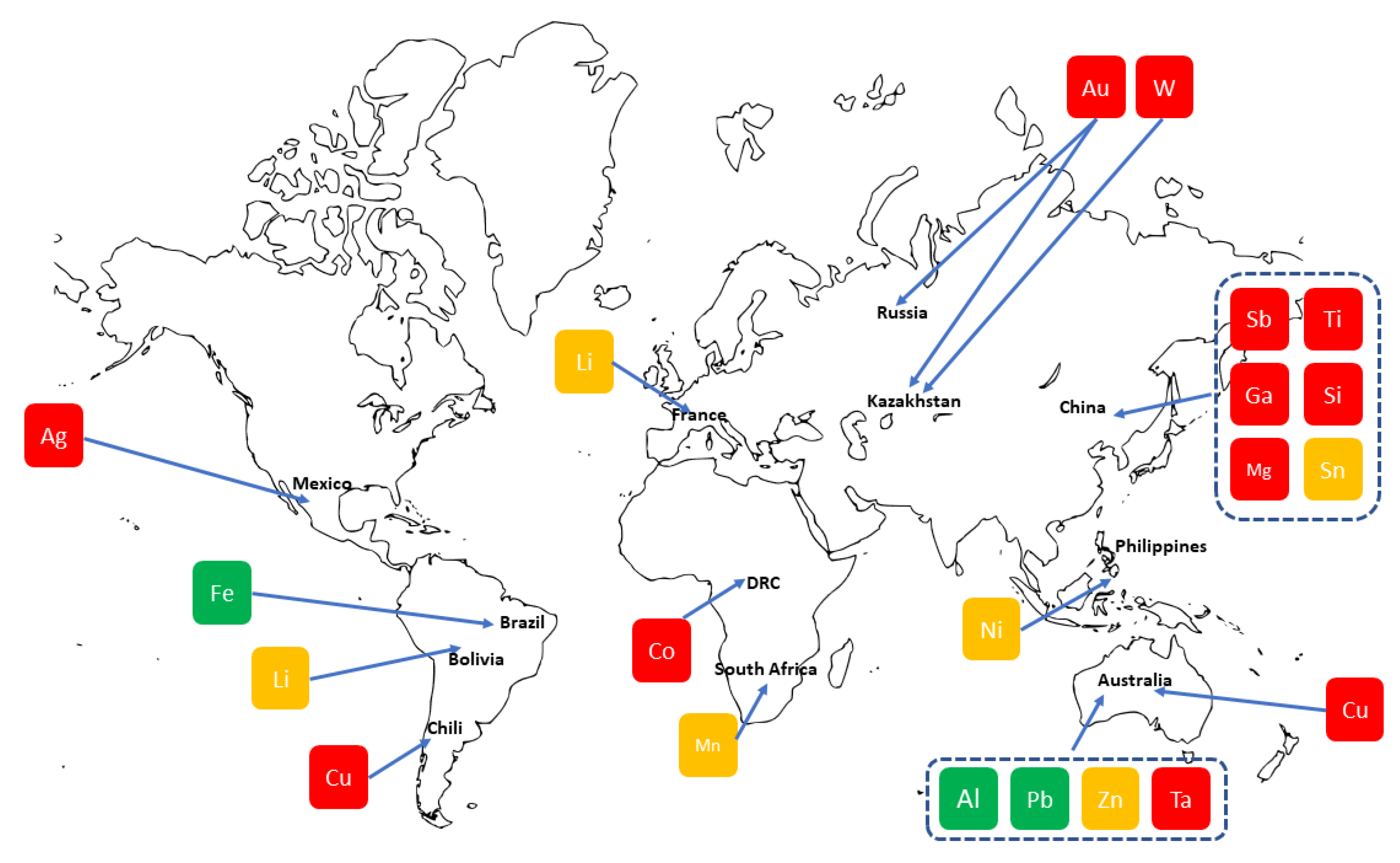
Figure 9.
Types of solders: (measured in the lab).
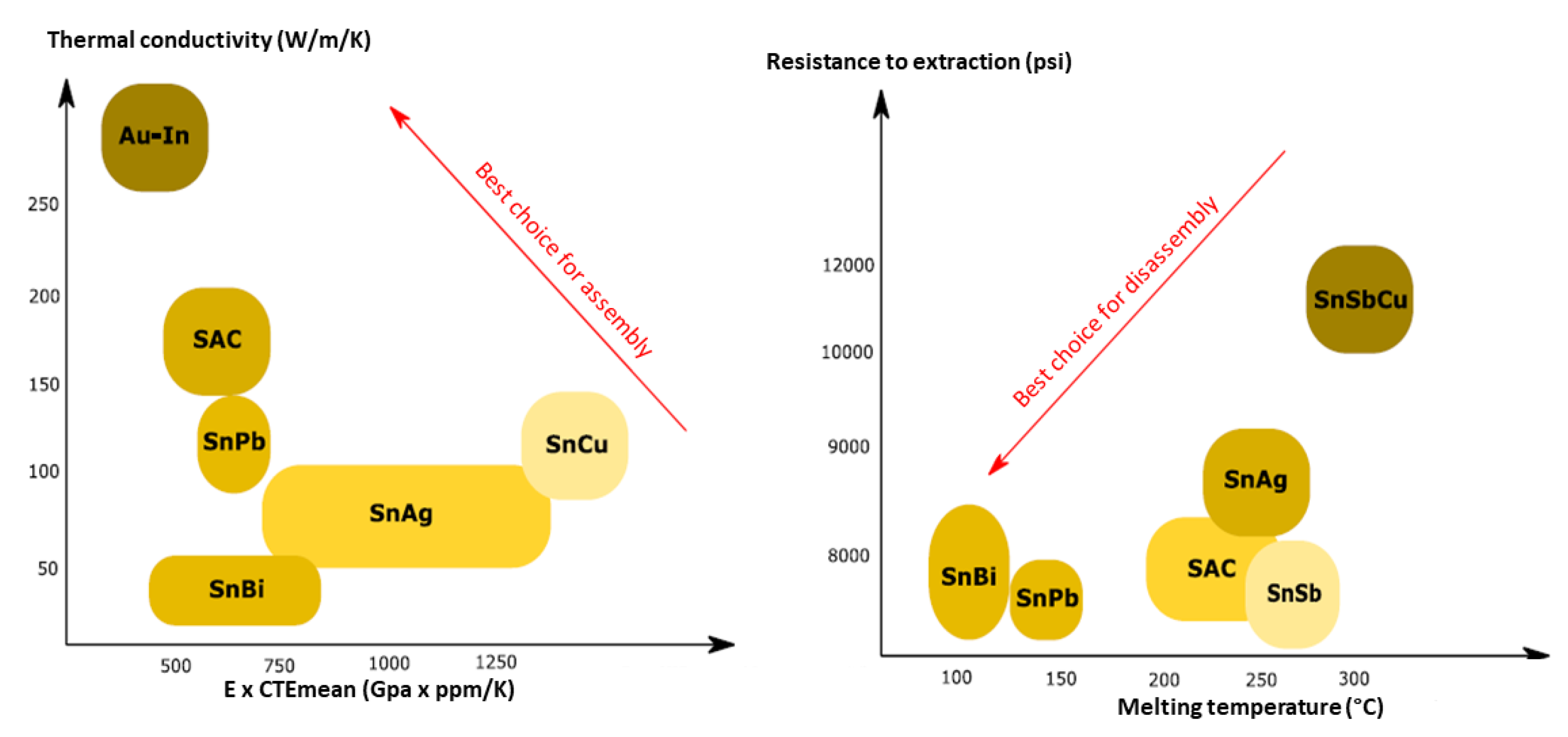
Figure 10.
Types of soldering flux, used to accelerate the soldering and avoid oxydation.
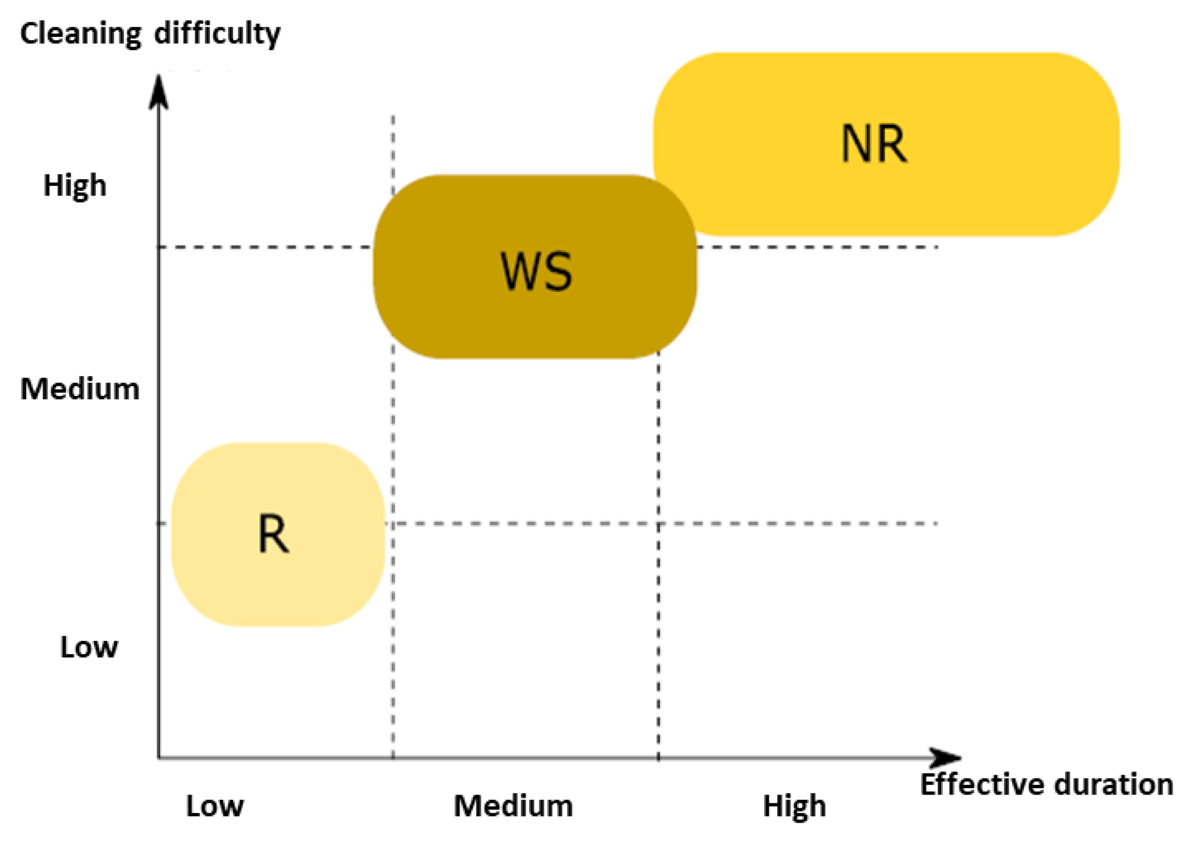
Table 1.
Condition monitoring methods.
| Type of Condition Monitoring Methods | The Method | Measured Quantity |
|---|---|---|
| Electrical methods: in contact with the Component | Saturation current | Vce-Vds |
| Threshold gate voltage | Vge-Vgs | |
| On voltage | Vce-Vd | |
| Di/dt variation | The device’s current | |
| Thermal methods (with a sensor) | Thermal analysis chip (TTC) | Thermal resistance |
| Acoustic methods (no contact) | Acoustic waves | Wavelength or harmonic distortions |
| Optical methods (no contact) | photodiodes sensors | Light intensity |
| Infrared camera | wavelength |
Disclaimer/Publisher’s Note: The statements, opinions and data contained in all publications are solely those of the individual author(s) and contributor(s) and not of MDPI and/or the editor(s). MDPI and/or the editor(s) disclaim responsibility for any injury to people or property resulting from any ideas, methods, instructions or products referred to in the content. |
© 2025 by the authors. Licensee MDPI, Basel, Switzerland. This article is an open access article distributed under the terms and conditions of the Creative Commons Attribution (CC BY) license (http://creativecommons.org/licenses/by/4.0/).
Copyright: This open access article is published under a Creative Commons CC BY 4.0 license, which permit the free download, distribution, and reuse, provided that the author and preprint are cited in any reuse.


