Unified Evolution Equation

1. Introduction

1.0. Proposal of the Unified Evolution Equation

(1)

Aim: What is the UEE?

The UEE series presents a common equation format for describing, as a single “time evolution of states (Schrödinger picture)”, the reversible dynamics of quantum systems (unitary evolution), dissipation as open systems (coarse-graining and measurement), and transport arising from boundaries and resonances (including the exact elimination of area terms). This time-evolution scheme is called the Unified Evolution Equation (UEE).

The standpoint of this paper is to first define the UEE without inconsistency as an analytical foundation. Accordingly, in this section we clarify the “proposal content” of the UEE with a minimal set of formulas, while detailed mathematical definitions (types of state spaces, CPTP properties, semigroups, generators, and closure under limits) are axiomatized step by step in the subsequent sections (§1.1–§1.4).

(2)

Abstract form in UEE_01 (as an analytical contract)

In UEE_01, the observable algebra is taken to be a von Neumann algebra $\mathfrak{M}$, and the state space its predual ${\mathfrak{M}}_{*}$. The time evolution of a state $\rho \left(t\right)\in {\mathfrak{M}}_{*}$ is expressed in the following formal differential form:

$$\dot{\rho }\left(t\right)={\mathcal{L}}_{\mathrm{tot}}\left[\rho \left(t\right)\right],{\mathcal{L}}_{\mathrm{tot}}:={\mathcal{L}}_0+{\mathcal{L}}_{\Delta }+R.$$

(1)

Here ${\mathcal{L}}_0$ denotes the reversible (unitary) component, ${\mathcal{L}}_{\Delta }$ the dissipative component, and R the zero-area resonance (transport) component. In this paper, (1) is presented as the “central equation”; however, since generators generally come with domains, the precise meaning of (1) is given as a mild solution (semigroup action)

$$\rho \left(t\right)=T_{\mathrm{tot}}\left(t\right)\left[{\rho }_0\right](t\ge 0)$$

generated by a strongly continuous CPTP (completely positive and trace-preserving) semigroup ${\left\{T_{\mathrm{tot}}\left(t\right)\right\}}_{t\ge 0}$ (the definition is given in §1.2). By this “definition as a semigroup,” state requirements such as positivity and normalization (trace preservation) are structurally guaranteed not to be violated under time evolution.

(3)

Standard representation used from UEE_05 onward (density-matrix representation)

In subsequent papers (UEE_05 and later), it is common to adopt the standard representation $\mathfrak{M}=\mathcal{B}\left(\mathcal{H}\right)$ and ${\mathfrak{M}}_{*}={\mathcal{T}}_1\left(\mathcal{H}\right)$ (where ${\mathcal{T}}_1$ denotes the trace class), and to represent $\rho \left(t\right)$ as a density operator (density matrix). In this case, (1) is typically written in the following common form:

$$\dot{\rho }\left(t\right)=-i[H,\rho \left(t\right)]+\sum _k\left(L_k\rho \left(t\right)L_k^{†}-\frac{1}{2}\{L_k^{†}{L}_k,\rho \left(t\right)\}\right)+R\left[\rho \left(t\right)\right].$$

(2)

That is, the reversible component is given by the commutator $-i[H,·]$ (a derivation), the dissipative component by a GKLS (Lindblad) generator, and R is placed alongside as a zero-area resonance generator. Moreover, in UEE_05 and later, a representation is frequently used in which, employing a family of measurement projections $\left\{{\mathrm{\Pi }}_n\right\}$, one sets $V_n=\sqrt{\gamma }{\mathrm{\Pi }}_n$ (minimal-rank GKLS), and the dissipation is given by ${\sum }_n\left(V_n\rho V_n^{†}-{\displaystyle \frac{1}{2}}\{V_n^{†}{V}_n,\rho \}\right)$. Furthermore, in UEE_05 and later, the minimal set of building blocks supporting this common form is treated collectively as D (reversible derivation), $\left\{{\mathrm{\Pi }}_n\right\}$ (pointer projection family), $\left\{V_n\right\}$ (Kraus operators), $\mathrm{\Phi }$ (normalization map), and R (zero-area resonance kernel) (the notation S5).

In the notation of this paper, the first term of (2) corresponds to ${\mathcal{L}}_0$, the entire second term to ${\mathcal{L}}_{\Delta }$, and R is treated as the same component.

(4)

Standpoint of this paper: fixing the proposal as an analytical foundation

What this paper addresses is not the derivation of the UEE from “physical motivations,” but rather the fixing of the UEE as a minimal analytically tractable contract and the guarantee, under that contract, that the UEE is well posed (existence, uniqueness, and invariance of states). In the next section §1.1, we clarify the input contracts to be fixed and the properties to be guaranteed by this paper; in §1.2 we declare the analytical objects; in §1.3 we state the main results; and in §1.4 we provide a roadmap of the paper structure.

1.1. Role of This Paper

(1)

Contract as an analytical foundation: what this paper “fixes” and “guarantees”

The role of this paper is to define the Unified Evolution Equation (UEE) as a mathematically consistent “time evolution of states (Schrödinger picture)” and to clarify the minimal requirements that make it analytically interpretable. More concretely, when the UEE is given in the form

$$\dot{\rho }\left(t\right)={\mathcal{L}}_{\mathrm{tot}}\left[\rho \left(t\right)\right],$$

this paper rigorously demonstrates, in a self-contained manner within the text, (i) on which space $\rho \left(t\right)$ should be treated (the type of the state space), (ii) the minimal conditions that each component constituting the generator ${\mathcal{L}}_{\mathrm{tot}}$ must satisfy (input contracts), and (iii) that, under those conditions, the time evolution $t\mapsto \rho \left(t\right)$ is uniquely determined and that the requirements for states (positivity, normalization, trace preservation corresponding to information conservation, etc.) are not violated (well-posedness and invariance).

Since this paper is a “foundational analytical paper,” the following are clearly separated and excluded from its scope:

• Derivation of equivalence between representations such as operator, variational, and field forms (in this paper, the operator form as the analytical input is fixed).
• Concrete phenomenology, numerical fitting, and identification of physical constants (the focus is on establishing definitions and theorems as an analytical foundation).
• Detailed geometric constructions (e.g., concrete flows on spacetime or measure-theoretic constructions); these are introduced only as abstract specifications when necessary and are formalized only to the extent required for the analytical claims.

(2)

Input of this paper: observable algebra, state space, and dynamical data (input contract)

This paper is based on the duality between observables (Heisenberg picture) and states (Schrödinger picture), and fixes the state space as the “predual of the algebra.” On this basis, the analytical input (data) of the UEE is defined uniquely.

Definition 1 (Observable algebra and state space (predual)).

Let $\mathfrak{M}$ be a von Neumann algebra, and let its predual be denoted by ${\mathfrak{M}}_{*}$. We write the unit of $\mathfrak{M}$ as $\mathbf{1}$.

1.

Positive functional: A functional $\rho \in {\mathfrak{M}}_{*}$ is said to be positive if $\rho \left(A\right)\ge 0$ holds for any positive operator $A\in \mathfrak{M}$ ($A\ge 0$).

2.

Normal state: A functional $\rho \in {\mathfrak{M}}_{*}$ is called a normal state if it is positive and satisfies $\rho \left(\mathbf{1}\right)=1$. The set of all normal states is denoted by $\mathcal{S}\left(\mathfrak{M}\right)$.

Hereafter, the time evolution of states is defined as a family of maps on ${\mathfrak{M}}_{*}$, and the UEE is described as its generator.

Definition 2 (UEE analytical data (minimal form of the input contract)).

The UEE analytical data in this paper is the tuple

$$\mathsf{D}:=(\mathfrak{M},{\mathfrak{M}}_{*},D,{\mathcal{L}}_{\Delta },R),$$

which satisfies the following:

1.

D is self-adjoint data generating the reversible (unitary) component, and ${\mathcal{L}}_0:=-i[D,·]$ is defined (as a linear operator on ${\mathfrak{M}}_{*}$ under an appropriate domain).

2.

${\mathcal{L}}_{\Delta }$ is the generator representing the dissipative component (measurement and coarse-graining), and generates, on ${\mathfrak{M}}_{*}$, a completely positive and trace-preserving (CPTP, defined below) semigroup (details are axiomatized and constructed in subsequent sections of the text).

3.

R is the generator representing the resonance and transport component, and generates a CPTP semigroup on ${\mathfrak{M}}_{*}$.

• Remark (fixing of types)

In this paper, D is (typically) introduced as an operator on a Hilbert space, whereas ${\mathcal{L}}_{\Delta }$ and R are generators (superoperators) on ${\mathfrak{M}}_{*}$. Accordingly, we do not add D and R as objects of the same type (e.g., we do not write $D+R$). Addition is always performed only at the level of generators, as

$${\mathcal{L}}_{\mathrm{tot}}:={\mathcal{L}}_0+{\mathcal{L}}_{\Delta }+R.$$

(3)

Minimal definition of CPTP (completely positive and trace-preserving) and immediate consequences (with proofs)

In this paper, the condition that the time evolution of states is “physically admissible” is formalized as CPTP (completely positive and trace-preserving). Normality of maps on a von Neumann algebra is fixed in order to ensure the well-definedness of the predual maps.

Definition 3 (Normal, completely positive, unital maps and preduals).

Let $\alpha :\mathfrak{M}\to \mathfrak{M}$ be a linear map.

1.

Normality: The map α is said to be normal if, for any increasing bounded net of positive operators $0\le A_i\uparrow A$ in $\mathfrak{M}$, one has $\alpha \left(A_i\right)\uparrow \alpha \left(A\right)$.

2.

Complete positivity: The map α is said to be completely positive (CP) if, for any $n\in \mathbb{N}$, ${\mathrm{id}}_{M_n}\otimes \alpha$ maps positive operators on $M_n\left(\mathbb{C}\right)\overline{\otimes }\mathfrak{M}$ to positive operators.

3.

Unitality: If $\alpha \left(\mathbf{1}\right)=\mathbf{1}$ holds, α is said to be unital.

4.

Predual map: If α is normal, its predual ${\alpha }_{*}:{\mathfrak{M}}_{*}\to {\mathfrak{M}}_{*}$ is defined by

$$\left({\alpha }_{*}\rho \right)\left(A\right):=\rho \left(\alpha \left(A\right)\right)(\rho \in {\mathfrak{M}}_{*},A\in \mathfrak{M}).$$

Lemma 1 (The predual of a unital CP map preserves states).

Let $\alpha :\mathfrak{M}\to \mathfrak{M}$ be normal, completely positive, and unital. Then its predual ${\alpha }_{*}:{\mathfrak{M}}_{*}\to {\mathfrak{M}}_{*}$ preserves the set of normal states, and

$${\alpha }_{*}\left(\mathcal{S}\left(\mathfrak{M}\right)\right)\subset \mathcal{S}\left(\mathfrak{M}\right)$$

holds.

Proof. 

Take an arbitrary $\rho \in \mathcal{S}\left(\mathfrak{M}\right)$. What must be shown is (i) that ${\alpha }_{*}\rho$ is positive, and (ii) that $\left({\alpha }_{*}\rho \right)\left(\mathbf{1}\right)=1$.

(i) Positivity: Let $A\in \mathfrak{M}$ be arbitrary with $A\ge 0$. By complete positivity (in particular, positivity), we have $\alpha \left(A\right)\ge 0$. Since $\rho$ is a positive functional, $\rho \left(\alpha \right(A\left)\right)\ge 0$ holds. By the definition of the predual in Definition 3,

$$\left({\alpha }_{*}\rho \right)\left(A\right)=\rho \left(\alpha \left(A\right)\right).$$

Therefore $\left({\alpha }_{*}\rho \right)\left(A\right)\ge 0$ holds for all $A\ge 0$, and ${\alpha }_{*}\rho$ is positive.

(ii) Normalization: By unitality, $\alpha \left(\mathbf{1}\right)=\mathbf{1}$. Hence, by the definition of the predual,

$$\left({\alpha }_{*}\rho \right)\left(\mathbf{1}\right)=\rho \left(\alpha \left(\mathbf{1}\right)\right)=\rho \left(\mathbf{1}\right)=1.$$

Thus ${\alpha }_{*}\rho \in \mathcal{S}\left(\mathfrak{M}\right)$ follows. □

Lemma 2 

(Composition of normal unital CP maps belongs to the same class). Let $\alpha ,\beta :\mathfrak{M}\to \mathfrak{M}$ both be normal, completely positive, and unital. Then their composition $\alpha \circ \beta$ is also normal, completely positive, and unital. Moreover, for the preduals,

$${(\alpha \circ \beta )}_{*}={\beta }_{*}\circ {\alpha }_{*}$$

holds.

Proof. 

(i) Unitality:.

$$(\alpha \circ \beta )\left(\mathbf{1}\right)=\alpha \left(\beta \right(\mathbf{1}\left)\right)=\alpha \left(\mathbf{1}\right)=\mathbf{1}.$$

(ii) Complete positivity: Take an arbitrary $n\in \mathbb{N}$. On $M_n\left(\mathbb{C}\right)\overline{\otimes }\mathfrak{M}$,

$${\mathrm{id}}_{M_n}\otimes (\alpha \circ \beta )=\left({\mathrm{id}}_{M_n}\otimes \alpha \right)\circ \left({\mathrm{id}}_{M_n}\otimes \beta \right)$$

holds. Since ${\mathrm{id}}_{M_n}\otimes \beta$ maps positive operators to positive operators, and ${\mathrm{id}}_{M_n}\otimes \alpha$ does likewise, their composition also maps positive operators to positive operators. Hence $\alpha \circ \beta$ is completely positive.

(iii) Normality: Take an increasing bounded net of positive operators $0\le A_i\uparrow A$. Since $\beta$ is normal, $\beta \left(A_i\right)\uparrow \beta \left(A\right)$. Since $\alpha$ is normal, $\alpha \left(\beta \left(A_i\right)\right)\uparrow \alpha \left(\beta \left(A\right)\right)$. Therefore $(\alpha \circ \beta )\left(A_i\right)\uparrow (\alpha \circ \beta )\left(A\right)$, and $\alpha \circ \beta$ is normal.

(iv) Composition formula for the preduals: For arbitrary $\rho \in {\mathfrak{M}}_{*}$ and $A\in \mathfrak{M}$, by Definition 3,

$$\left(({\beta }_{*}\circ {\alpha }_{*})\rho \right)\left(A\right)=\left({\alpha }_{*}\rho \right)\left(\beta \left(A\right)\right)=\rho \left(\alpha \left(\beta \right(A\left)\right)\right)=\rho \left((\alpha \circ \beta )\left(A\right)\right)=\left({(\alpha \circ \beta )}_{*}\rho \right)\left(A\right).$$

Hence they coincide as functionals, and ${(\alpha \circ \beta )}_{*}={\beta }_{*}\circ {\alpha }_{*}$ follows. □

(4)

Destination of this paper (conclusion of this subsection) and connection to subsequent sections

From the above, this paper has formulated “physically admissible time evolution” as the predual of normal, unital CP maps on a von Neumann algebra, and has shown (within this subsection) that the state set $\mathcal{S}\left(\mathfrak{M}\right)$ is automatically invariant. In the subsequent sections, from each component of the UEE analytical data (Definition 2), we construct

$${\mathcal{L}}_{\mathrm{tot}}:={\mathcal{L}}_0+{\mathcal{L}}_{\Delta }+R,$$

obtain a strongly continuous CPTP semigroup $T\left(t\right)$ as the composite limit of component semigroups, and prove that $\rho \left(t\right)=T\left(t\right)\left[{\rho }_0\right]$ is the rigorous (mild) solution of the UEE.

1.2. Declaration of Analytical Objects

(1)

Position of this subsection: fixing the “types” and “objects” on which all subsequent discussions rely

In this subsection, in order to treat the Unified Evolution Equation (UEE) as a mathematical object, we declare, in a way that prevents any confusion of types, (i) the stage (observable algebra and state space), (ii) the dynamics (a family of time-evolution maps), and (iii) the generator (the right-hand side of the differential equation). In particular, as a “foundational analytical paper,” this paper fixes the analytical objects of the UEE with minimal specifications so that the subsequent discussions of existence, uniqueness, and conservation laws do not break down due to ambiguity of definitions or mixing of operator types.

(2)

Definition of the UEE-Analytic Datum: fixing the input contract

The UEE is described by a generator (superoperator) ${\mathcal{L}}_{\mathrm{tot}}$ that gives the time evolution of a state $\rho \left(t\right)$. In this paper, the input required for the analysis of the UEE is defined as the following tuple.

Definition 4 

(UEE-Analytic Datum). The analytical datum of the UEE (UEE-Analytic Datum) is a tuple

$$\mathsf{D}:=(\mathfrak{M},{\mathfrak{M}}_{*},D,{\mathcal{L}}_{\Delta },R),$$

which satisfies the following:

1.

Observable algebra and state space: $\mathfrak{M}$ is a von Neumann algebra, and ${\mathfrak{M}}_{*}$ is its predual. The set of normal states is defined by

$$\mathcal{S}\left(\mathfrak{M}\right):=\{\rho \in {\mathfrak{M}}_{*}:\rho \ge 0,\rho \left(\mathbf{1}\right)=1\}.$$

2.

Reversible component:D is given (in the standard realization $\mathfrak{M}=B\left(\mathcal{H}\right)$) as a self-adjoint operator on a Hilbert space, and, via the unitary conjugation group defined later, yields a reversible (CPTP) time evolution on the state space.

3.

Dissipative component: ${\mathcal{L}}_{\Delta }$ is a linear operator on the state space ${\mathfrak{M}}_{*}$, and generates a completely positive and trace-preserving (CPTP) strongly continuous semigroup.

4.

Transport (resonance) component: R is a linear operator on the state space ${\mathfrak{M}}_{*}$, and generates a CPTP strongly continuous semigroup.

• Remark (prohibited type operations)

While D is given (in the standard realization) as an operator on a Hilbert space, ${\mathcal{L}}_{\Delta }$ and R are generators (superoperators) on the state space ${\mathfrak{M}}_{*}$. Accordingly, in this paper we never add D and R as objects of the same type (e.g., we never write $D+R$). Hereafter, addition is performed only among generators, and the total generator is defined by

$${\mathcal{L}}_{\mathrm{tot}}:={\mathcal{L}}_0+{\mathcal{L}}_{\Delta }+R\left({\mathcal{L}}_0\mathrm{will}\mathrm{be}\mathrm{given}\mathrm{later}\right).$$

(3)

Time-evolution family and generator of the UEE: formulation as an abstract Cauchy problem

This paper treats the UEE as an abstract Cauchy problem on the Banach space $X:={\mathfrak{M}}_{*}$. For this purpose, we define strongly continuous semigroups and their generators.

Definition 5 (Strongly continuous semigroup and generator).

Let X be a Banach space, and let ${\left\{T\left(t\right)\right\}}_{t\ge 0}$ be a family of linear operators on X.

1.

The family ${\left\{T\left(t\right)\right\}}_{t\ge 0}$ is called a  strongly continuous semigroup ($C_0$-semigroup) if

$$T\left(0\right)=I,T(t+s)=T\left(t\right)T\left(s\right)(\forall t,s\ge 0)$$

and for every $x\in X$,

$$\underset{t\downarrow 0}{lim}{\parallel T\left(t\right)x-x\parallel }_X=0$$

holds.

2.

The generator A of ${\left\{T\left(t\right)\right\}}_{t\ge 0}$ is defined by taking as its domain $\mathrm{Dom}\left(A\right)$ the set of all $x\in X$ for which the limit

$$Ax:=\underset{t\downarrow 0}{lim}{\displaystyle \frac{T\left(t\right)x-x}{t}}$$

exists.

• Abstract form of the UEE

The UEE treated in this paper is (formally) given by

$${\displaystyle \frac{d}{dt}}\rho \left(t\right)={\mathcal{L}}_{\mathrm{tot}}\left[\rho \left(t\right)\right]\left(\rho \left(0\right)={\rho }_0\in \mathcal{S}\left(\mathfrak{M}\right)\right).$$

However, from the analytical standpoint of this paper, we allow that the domain of ${\mathcal{L}}_{\mathrm{tot}}$ does not, in general, coincide with the whole space, and we adopt as the basic notion that the solution is first given by a strongly continuous semigroup $T\left(t\right)$ as

$$\rho \left(t\right):=T\left(t\right)\left[{\rho }_0\right]$$

(the so-called mild solution). With this criterion of “mild solution = semigroup action,” we can address the domain issue head-on without evading it.

(4)

Basic lemmas in the standard realization ($B\left(\mathcal{H}\right)$ and trace class): CPTP property and strong continuity of the reversible component

In order to complete the proofs within the paper, we henceforth adopt, as the main stage, the standard realization

$$\mathfrak{M}=B\left(\mathcal{H}\right),{\mathfrak{M}}_{*}={\mathcal{T}}_1\left(\mathcal{H}\right)$$

(trace-class operators). Here the reversible component ${\mathcal{L}}_0$ is determined by unitary conjugation generated by a self-adjoint operator D. We prove its properties (CPTP, isometry, and strong continuity) within this subsection, without depending on later sections.

First, we fix basic facts about the trace and the trace norm.

Lemma 3 (Cyclicity for products of a trace-class operator and a bounded operator).

Let $\mathcal{H}$ be a complex Hilbert space, and let $A\in B\left(\mathcal{H}\right)$ and $B\in {\mathcal{T}}_1\left(\mathcal{H}\right)$. Then $AB,BA\in {\mathcal{T}}_1\left(\mathcal{H}\right)$, and

$$\mathrm{Tr}\left(AB\right)=\mathrm{Tr}\left(BA\right)$$

holds.

Proof. Step 1 (finite-rank case): 

Assume that B is a finite-rank operator. A finite-rank operator can be written as a finite sum

$$B=\sum _{k=1}^n|{\psi }_k\rangle \langle {\varphi }_k|({\psi }_k,{\varphi }_k\in \mathcal{H}).$$

Then

$$AB=\sum _{k=1}^n|A{\psi }_k\rangle \langle {\varphi }_k|,BA=\sum _{k=1}^n|{\psi }_k\rangle \langle A^{*}{\varphi }_k|$$

and both are trace class since they are finite rank. Moreover, for a rank-one operator $|\psi \rangle \langle \varphi |$,

$$\mathrm{Tr}\left(|\psi \rangle \langle \varphi |\right)=\langle \varphi ,\psi \rangle$$

holds (for an orthonormal basis $\left\{e_j\right\}$, ${\sum }_j\langle e_j,|\psi \rangle \langle \varphi |e_j\rangle ={\sum }_j\langle e_j,\psi \rangle \langle \varphi ,e_j\rangle =\langle \varphi ,\psi \rangle$). Hence

$$\begin{array}{cc}\hfill \mathrm{Tr}\left(AB\right)& =\sum _{k=1}^n\mathrm{Tr}\left(|A{\psi }_k\rangle \langle {\varphi }_k|\right)=\sum _{k=1}^n\langle {\varphi }_k,A{\psi }_k\rangle ,\hfill \\ \hfill \mathrm{Tr}\left(BA\right)& =\sum _{k=1}^n\mathrm{Tr}\left(|{\psi }_k\rangle \langle A^{*}{\varphi }_k|\right)=\sum _{k=1}^n\langle A^{*}{\varphi }_k,{\psi }_k\rangle =\sum _{k=1}^n\langle {\varphi }_k,A{\psi }_k\rangle .\hfill \end{array}$$

Therefore $\mathrm{Tr}\left(AB\right)=\mathrm{Tr}\left(BA\right)$ holds for finite-rank B.

Step 2 (extension to general trace-class operators): In general, for $B\in {\mathcal{T}}_1\left(\mathcal{H}\right)$, by singular-value decomposition (Schmidt decomposition),

$$B=\sum _{k=1}^{\infty }{s}_k|{\psi }_k\rangle \langle {\varphi }_k|$$

with $\left\{s_k\right\}$ satisfying $s_k\ge 0$ and ${\sum }_k{s}_k<\infty$ (countability of the trace norm). The partial sums

$$B_N:=\sum _{k=1}^N{s}_k|{\psi }_k\rangle \langle {\varphi }_k|$$

are finite rank, and

$$\parallel B-B_N{\parallel }_1=\sum _{k>N}{s}_k⟶0(N\to \infty ).$$

For bounded A, by the ideal property of the trace norm,

$$\parallel A(B-B_N){\parallel }_1\le \parallel A\parallel \parallel B-B_N{\parallel }_1\to 0,\parallel (B-B_N){A\parallel }_1\le \parallel A\parallel \parallel B-B_N{\parallel }_1\to 0.$$

Hence $A{B}_N\to AB$ and $B_{N}A\to BA$ in trace norm. Since the trace is continuous with respect to the trace norm,

$$\mathrm{Tr}\left(AB\right)=\underset{N\to \infty }{lim}\mathrm{Tr}\left(A{B}_N\right),\mathrm{Tr}\left(BA\right)=\underset{N\to \infty }{lim}\mathrm{Tr}\left(B_{N}A\right).$$

By Step 1, $\mathrm{Tr}\left(A{B}_N\right)=\mathrm{Tr}\left(B_{N}A\right)$ for each N, and taking limits yields $\mathrm{Tr}\left(AB\right)=\mathrm{Tr}\left(BA\right)$. Moreover, the above estimates imply that $AB,BA$ are trace class. □

Next, we state explicitly the density of finite-rank operators (used in the proof of strong continuity).

Lemma 4 (Density of finite-rank operators).

The set of all finite-rank operators $\mathcal{F}\left(\mathcal{H}\right)$ is dense in ${\mathcal{T}}_1\left(\mathcal{H}\right)$. That is, for any $B\in {\mathcal{T}}_1\left(\mathcal{H}\right)$ and any $\epsilon >0$, there exists $B_{\epsilon }\in \mathcal{F}\left(\mathcal{H}\right)$ such that

$$\parallel B-B_{\epsilon }{\parallel }_1<\epsilon .$$

Proof. 

Take an arbitrary $B\in {\mathcal{T}}_1\left(\mathcal{H}\right)$. By singular-value decomposition,

$$B=\sum _{k=1}^{\infty }{s}_k|{\psi }_k\rangle \langle {\varphi }_k|,s_k\ge 0,\sum _{k=1}^{\infty }{s}_k={\parallel B\parallel }_1<\infty .$$

The partial sums $B_N:={\sum }_{k=1}^N{s}_k|{\psi }_k\rangle \langle {\varphi }_k|$ are finite rank, and

$$\parallel B-B_N{\parallel }_1=\sum _{k>N}{s}_k\to 0(N\to \infty ).$$

Therefore, for a given $\epsilon >0$, choosing sufficiently large N yields $\parallel B-B_N{\parallel }_1<\epsilon$. □

Using these, we show that the reversible component is proper as an “analytical object.”

Theorem 1 (CPTP property, isometry, and strong continuity of the unitary conjugation group).

Let D be a self-adjoint operator on $\mathcal{H}$, and let $U\left(t\right):=e^{-itD}$ ($t\in \mathbb{R}$) be the unitary group given by Stone’s theorem. Define a family of maps ${\left\{T_0\left(t\right)\right\}}_{t\in \mathbb{R}}$ on $X:={\mathcal{T}}_1\left(\mathcal{H}\right)$ by

$$T_0\left(t\right)\left[\rho \right]:=U\left(t\right)\rho U{\left(t\right)}^{*}(\rho \in X).$$

Then the following hold:

1.

(CPTP) For each t, $T_0\left(t\right)$ is completely positive and trace-preserving.

2.

(Group property)$T_0(t+s)=T_0\left(t\right)\circ T_0\left(s\right)$, $T_0\left(0\right)=I$, and $T_0{\left(t\right)}^{-1}=T_0(-t)$.

3.

(Isometry) For each t, $\parallel T_0{\left(t\right)\left[\rho \right]\parallel }_1={\parallel \rho \parallel }_1$.

4.

(Strong continuity) For any $\rho \in X$, $\parallel T_0{\left(t\right)\left[\rho \right]-\rho \parallel }_1\to 0$ as $t\to 0$.

Therefore, ${\left\{T_0\left(t\right)\right\}}_{t\in \mathbb{R}}$ is a strongly continuous isometric CPTP group on X, and in particular preserves the normal state set $\mathcal{S}\left(B\right(\mathcal{H}\left)\right)$.

Proof. (1) CPTP:

First we show that $T_0\left(t\right)$ is well-defined on X. Since $U\left(t\right)\in B\left(\mathcal{H}\right)$ is bounded and $\rho \in {\mathcal{T}}_1\left(\mathcal{H}\right)$ is trace class, both $U\left(t\right)\rho$ and $\left(U\left(t\right)\rho \right)U{\left(t\right)}^{*}$ are trace class (the trace class is preserved under left and right multiplication by bounded operators). Hence $T_0\left(t\right):X\to X$ is well-defined.

Next we show trace preservation. Applying Lemma 3 with $A:=U{\left(t\right)}^{*}$ and $B:=U\left(t\right)\rho$ yields

$$\mathrm{Tr}\left(U\left(t\right)\rho U{\left(t\right)}^{*}\right)=\mathrm{Tr}\left(\rho U{\left(t\right)}^{*}U\left(t\right)\right)=\mathrm{Tr}\left(\rho \right).$$

Thus $T_0\left(t\right)$ is trace-preserving.

Next we show complete positivity. For any $n\in \mathbb{N}$, on ${\mathcal{H}}_n:={\mathbb{C}}^n\otimes \mathcal{H}$, $\tilde{U}\left(t\right):=I_n\otimes U\left(t\right)$ is unitary. Identifying $M_n\left(\mathbb{C}\right)\otimes {\mathcal{T}}_1\left(\mathcal{H}\right)$ with ${\mathcal{T}}_1\left({\mathcal{H}}_n\right)$, ${\mathrm{id}}_n\otimes T_0\left(t\right)$ is given by

$$({\mathrm{id}}_n\otimes T_0\left(t\right))\left[\tilde{\rho }\right]=\tilde{U}\left(t\right)\tilde{\rho }\tilde{U}{\left(t\right)}^{*}(\tilde{\rho }\in {\mathcal{T}}_1\left({\mathcal{H}}_n\right)).$$

If $\tilde{\rho }\ge 0$, then for any $\xi \in {\mathcal{H}}_n$,

$$\langle \xi ,\tilde{U}\left(t\right)\tilde{\rho }\tilde{U}{\left(t\right)}^{*}\xi \rangle =\langle \tilde{U}{\left(t\right)}^{*}\xi ,\tilde{\rho }\tilde{U}{\left(t\right)}^{*}\xi \rangle \ge 0,$$

so $\tilde{U}\left(t\right)\tilde{\rho }\tilde{U}{\left(t\right)}^{*}\ge 0$. Hence ${\mathrm{id}}_n\otimes T_0\left(t\right)$ preserves positivity, and $T_0\left(t\right)$ is completely positive. Therefore $T_0\left(t\right)$ is CPTP.

(2) Group property: By the unitary-group identities $U(t+s)=U\left(t\right)U\left(s\right)$ and $U\left(0\right)=I$, for any $\rho \in X$,

$$T_0(t+s)\left[\rho \right]=U(t+s)\rho U{(t+s)}^{*}=U\left(t\right)U\left(s\right)\rho U{\left(s\right)}^{*}U{\left(t\right)}^{*}=T_0\left(t\right)\left[T_0\left(s\right)\left[\rho \right]\right]$$

holds. Thus $T_0(t+s)=T_0\left(t\right)\circ T_0\left(s\right)$, and $T_0\left(0\right)=I$. Moreover, since $U{\left(t\right)}^{-1}=U{\left(t\right)}^{*}=U(-t)$, we have $T_0{\left(t\right)}^{-1}=T_0(-t)$.

(3) Isometry (trace-norm invariance): Take an arbitrary $\rho \in X$. The trace norm is defined by ${\parallel \rho \parallel }_1=\mathrm{Tr}(|\rho |)$. Let $|A|:={\left(A^{*}A\right)}^{1/2}$. First,

$${\left(T_0\left(t\right)\left[\rho \right]\right)}^{*}{T}_0\left(t\right)\left[\rho \right]={\left(U\rho U^{*}\right)}^{*}\left(U\rho U^{*}\right)=U{\rho }^{*}{U}^{*}U\rho U^{*}=U\left({\rho }^{*}\rho \right)U^{*}={U(|\rho |}^2)U^{*},$$

hence

$$\left|T_0\left(t\right)\left[\rho \right]\right|={\left({U|\rho |}^2{U}^{*}\right)}^{1/2}=U|\rho |U^{*}$$

by uniqueness of the square root and unitarity of U. Therefore, using Lemma 3,

$$\parallel T_0{\left(t\right)\left[\rho \right]\parallel }_1=\mathrm{Tr}\left(|T_0\left(t\right)\left[\rho \right]|\right)=\mathrm{Tr}(U|\rho |U^{*})=\mathrm{Tr}(|\rho |U^{*}{U)=\mathrm{Tr}(|\rho |)=\parallel \rho \parallel }_1.$$

(4) Strong continuity: Take arbitrary $\rho \in X$ and $\epsilon >0$. By Lemma 4, choose a finite-rank ${\rho }_{\epsilon }$ such that

$$\parallel \rho -{\rho }_{\epsilon }{\parallel }_1<\epsilon .$$

By isometry,

$$\parallel T_0{\left(t\right)\left[\rho \right]-\rho \parallel }_1\le \parallel T_0\left(t\right)[\rho -{\rho }_{\epsilon }]{\parallel }_1+\parallel T_0\left(t\right)\left[{\rho }_{\epsilon }\right]-{\rho }_{\epsilon }{\parallel }_1+{\parallel {\rho }_{\epsilon }-\rho \parallel }_1$$

$$=2\parallel \rho -{\rho }_{\epsilon }{\parallel }_1+\parallel T_0\left(t\right)\left[{\rho }_{\epsilon }\right]-{\rho }_{\epsilon }{\parallel }_1<2\epsilon +{\parallel T_0\left(t\right)\left[{\rho }_{\epsilon }\right]-{\rho }_{\epsilon }\parallel }_1.$$

Hence it suffices to show that $\parallel T_0\left(t\right)\left[{\rho }_{\epsilon }\right]-{\rho }_{\epsilon }{\parallel }_1\to 0$ as $t\to 0$.

A finite-rank ${\rho }_{\epsilon }$ can be written as

$${\rho }_{\epsilon }=\sum _{k=1}^N|{\psi }_k\rangle \langle {\varphi }_k|.$$

Thus

$$T_0\left(t\right)\left[{\rho }_{\epsilon }\right]-{\rho }_{\epsilon }=\sum _{k=1}^N\left(|U\left(t\right){\psi }_k\rangle \langle U\left(t\right){\varphi }_k|-|{\psi }_k\rangle \langle {\varphi }_k|\right).$$

Each term can be decomposed as

$$|U\psi \rangle \langle U\varphi |-|\psi \rangle \langle \varphi |=\left(|U\psi \rangle -|\psi \rangle \right)\langle U\varphi |+|\psi \rangle \left(\langle U\varphi |-\langle \varphi |\right),$$

which is an identity obtained by adding and subtracting. Since the trace norm of a rank-one operator $|\eta \rangle \langle \xi |$ is ${\parallel |\eta \rangle \langle \xi |\parallel }_1=\parallel \eta \parallel \parallel \xi \parallel$, by the triangle inequality,

$${∥|U\psi \rangle \langle U\varphi |-|\psi \rangle \langle \varphi |∥}_1\le \parallel U\left(t\right)\psi -\psi \parallel \parallel U\left(t\right)\varphi \parallel +\parallel \psi \parallel \parallel U\left(t\right)\varphi -\varphi \parallel .$$

By unitarity, $\parallel U\left(t\right)\varphi \parallel =\parallel \varphi \parallel$, so

$${∥|U\psi \rangle \langle U\varphi |-|\psi \rangle \langle \varphi |∥}_1\le \parallel U\left(t\right)\psi -\psi \parallel \parallel \varphi \parallel +\parallel \psi \parallel \parallel U\left(t\right)\varphi -\varphi \parallel .$$

Since $U\left(t\right)$ is strongly continuous on $\mathcal{H}$ (Stone’s theorem), $\parallel U\left(t\right)\psi -\psi \parallel \to 0$ and $\parallel U\left(t\right)\varphi -\varphi \parallel \to 0$ as $t\to 0$. Therefore, for each k,

$${∥|U\left(t\right){\psi }_k\rangle \langle U\left(t\right){\varphi }_k|-|{\psi }_k\rangle \langle {\varphi }_k|∥}_1\to 0(t\to 0).$$

Because the sum is finite, we can interchange limit and summation, obtaining

$$\parallel T_0\left(t\right)\left[{\rho }_{\epsilon }\right]-{\rho }_{\epsilon }{\parallel }_1\le \sum _{k=1}^N{∥|U\left(t\right){\psi }_k\rangle \langle U\left(t\right){\varphi }_k|-|{\psi }_k\rangle \langle {\varphi }_k|∥}_1\to 0(t\to 0).$$

Hence, for any $\epsilon >0$, taking t sufficiently small yields $\parallel T_0{\left(t\right)\left[\rho \right]-\rho \parallel }_1<3\epsilon$, proving strong continuity.

Finally, invariance of $\mathcal{S}\left(B\right(\mathcal{H}\left)\right)$ follows from the CPTP property. (Positivity and trace preservation were shown in (1).) □

(5)

Conclusion of this subsection: analytical objects (types, time evolution, generators) have been fixed

In this subsection, we declared the objects for treating the UEE analytically as (i) the observable algebra $\mathfrak{M}$ and the state space ${\mathfrak{M}}_{*}$, (ii) the analytical datum $\mathsf{D}=(\mathfrak{M},{\mathfrak{M}}_{*},D,{\mathcal{L}}_{\Delta },R)$, and (iii) the total generator ${\mathcal{L}}_{\mathrm{tot}}={\mathcal{L}}_0+{\mathcal{L}}_{\Delta }+R$, and prohibited any confusion of types. Moreover, in the standard realization, we proved within the text that the reversible component is well-defined as a strongly continuous CPTP group by Theorem 1. In the subsequent sections, we establish the generation of semigroups by the dissipative component ${\mathcal{L}}_{\Delta }$ and the transport component R, and, by composing them, we establish the well-posedness of the UEE (existence, uniqueness, and invariance of states).

1.3. Main Results

(1)

Aim of this subsection: explicitly stating the “minimal set” proved in this paper and fixing the dependency structure

In this subsection, we list the main results that this paper must establish as foundational analysis, in a form such that the proof structure of the subsequent sections can be reconstructed uniquely. The main results here are: (i) the reversible part, the dissipative part, and the transport (resonance) part each provide physically admissible time evolutions (CPTP), (ii) by their componentwise composition, the total generator

$${\mathcal{L}}_{\mathrm{tot}}:={\mathcal{L}}_0+{\mathcal{L}}_{\Delta }+R({\mathcal{L}}_0:=-i[D,·])$$

generates a strongly continuous CPTP semigroup, and the UEE solution (mild solution) exists uniquely, and (iii) the set of normal states is invariant for all times, in these three points.

The proofs concerning existence and identification of the generator in the main theorem are given in the subsequent sections (§3–§6) after preparing the required apparatus ($C_0$-semigroup theory, product formulas, common cores). On the other hand, in this subsection we completely prove, within the paper, the closure lemmas required for “CPTP is preserved under componentwise composition,” so that the subsequent proofs close without external references.

(2)

Re-declaration of the main objects: component semigroups and composite approximations

Hereafter, let the state space be a Banach space X (in the standard realization, $X={\mathcal{T}}_1\left(\mathcal{H}\right)$), with norm ${\parallel ·\parallel }_1$. We write the component semigroups as

$$T_0\left(t\right):=e^{t{\mathcal{L}}_0},T_{\Delta }\left(t\right):=e^{t{\mathcal{L}}_{\Delta }},T_R\left(t\right):=e^{tR}(t\ge 0)$$

(the precise definitions, CPTP properties, and strong continuity of each are given in subsequent sections).

Define the basic map for the composite approximation by

$$F\left(t\right):=T_0\left(t\right)T_{\Delta }\left(t\right)T_R\left(t\right)(t\ge 0),$$

and define the approximating semigroup sequence for an n-partition by

$$T^{\left(n\right)}\left(t\right):={\left(F(t/n)\right)}^n(t\ge 0,n\in \mathbb{N}).$$

The main theorem (stated below) asserts that the strong limit

$$T\left(t\right)\left[\rho \right]:=\underset{n\to \infty }{lim}{T}^{\left(n\right)}\left(t\right)\rho (\rho \in X)$$

exists, that ${\left\{T\left(t\right)\right\}}_{t\ge 0}$ is a strongly continuous CPTP semigroup, and that its generator coincides with $\overline{{\mathcal{L}}_{\mathrm{tot}}}$.

(3)

Closure of CPTP: CPTP is not destroyed by composition or by pointwise strong limits (complete proofs)

The key point that must be established first in this subsection is the closure property: “the composition of CPTP maps is CPTP, and moreover the pointwise strong limit preserves CPTP.” This secures the CPTP property of the limit semigroup obtained by a product formula, independently of generator identification.

Lemma 5 (Closure under composition of CPTP maps).

Let $X={\mathcal{T}}_1\left(\mathcal{H}\right)$. If $S,T:X\to X$ are CPTP, then the composition $S\circ T$ is also CPTP.

Proof. 

Trace preservation follows from linearity and $\mathrm{Tr}\left(S\right[T\left(\rho \right)\left]\right)=\mathrm{Tr}\left(T\right(\rho \left)\right)=\mathrm{Tr}\left(\rho \right)$. For complete positivity, take an arbitrary $n\in \mathbb{N}$ and note that

$${\mathrm{id}}_n\otimes (S\circ T)=({\mathrm{id}}_n\otimes S)\circ ({\mathrm{id}}_n\otimes T).$$

Since ${\mathrm{id}}_n\otimes T$ preserves positivity and ${\mathrm{id}}_n\otimes S$ also preserves positivity, their composition preserves positivity. Hence $S\circ T$ is completely positive. Therefore $S\circ T$ is CPTP. □

Lemma 6 (Closure of CPTP under pointwise strong limits).

Let $X={\mathcal{T}}_1\left(\mathcal{H}\right)$. Let ${\left\{T_n\right\}}_{n\in \mathbb{N}}$ be a sequence of linear maps such that each $T_n$ is CPTP, and suppose that for a linear map $T:X\to X$, for every $\rho \in X$,

$$\parallel T_n{\left(\rho \right)-T\left(\rho \right)\parallel }_1⟶0(n\to \infty )$$

holds. Then T is CPTP.

Proof. Step 1 (trace preservation): 

The trace functional is continuous with respect to ${\parallel ·\parallel }_1$, and concretely, for any $A\in X$,

$$|\mathrm{Tr}\left(A\right)|\le {\parallel A\parallel }_1$$

holds. Therefore, for any $\rho \in X$,

$$\mathrm{Tr}\left(T\left(\rho \right)\right)=\underset{n\to \infty }{lim}\mathrm{Tr}\left(T_n\left(\rho \right)\right)=\underset{n\to \infty }{lim}\mathrm{Tr}\left(\rho \right)=\mathrm{Tr}\left(\rho \right),$$

so T is trace-preserving.

Step 2 (complete positivity: amplification to matrix levels): Fix an arbitrary $k\in \mathbb{N}$ and set $X_k:={\mathcal{T}}_1({\mathbb{C}}^k\otimes \mathcal{H})$. Since $T_n$ is CPTP, for each n,

$${\tilde{T}}_n:={\mathrm{id}}_k\otimes T_n:X_k\to X_k$$

preserves positivity.

Now, any $Z\in X_k$ can be written using the matrix units ${\left\{E_{ij}\right\}}_{i,j=1}^k$ as

$$Z=\sum _{i,j=1}^k{E}_{ij}\otimes Z_{ij}(Z_{ij}\in X)$$

(a finite sum since k is finite). Then

$${\tilde{T}}_n\left(Z\right)-\tilde{T}\left(Z\right)=\sum _{i,j=1}^k{E}_{ij}\otimes \left(T_n\left(Z_{ij}\right)-T\left(Z_{ij}\right)\right),\tilde{T}:={\mathrm{id}}_k\otimes T.$$

Using the triangle inequality and the basic estimate for the tensor product in the trace norm,

$$\parallel E_{ij}{\otimes A\parallel }_1=\parallel E_{ij}{\parallel }_1{\parallel A\parallel }_1={\parallel A\parallel }_1(A\in X),$$

we obtain

$$\parallel {\tilde{T}}_n\left(Z\right)-\tilde{T}{\left(Z\right)\parallel }_1\le \sum _{i,j=1}^k{\parallel T_n\left(Z_{ij}\right)-T\left(Z_{ij}\right)\parallel }_1⟶0(n\to \infty ),$$

since the assumed convergence holds for each $Z_{ij}$ and the sum is finite (so we may interchange limit and sum).

Step 3 (closedness of the positive cone): The positive cone of $X_k$, $X_{k,+}:=\{Z\in X_k:Z\ge 0\}$, is closed with respect to ${\parallel ·\parallel }_1$. Indeed, if $\parallel A_n{-A\parallel }_1\to 0$, then $\parallel A_n-A\parallel \le \parallel A_n{-A\parallel }_1\to 0$ implies convergence also in operator norm. Since the positive cone is closed in operator norm, $A_n\ge 0$ implies $A\ge 0$.

Step 4 (conclusion of complete positivity): Take an arbitrary $Z\in X_{k,+}$. Then ${\tilde{T}}_n\left(Z\right)\ge 0$ holds for all n (positivity preservation of ${\tilde{T}}_n$). By Step 2, $\parallel {\tilde{T}}_n\left(Z\right)-\tilde{T}{\left(Z\right)\parallel }_1\to 0$, so Step 3 (closedness) implies $\tilde{T}\left(Z\right)\ge 0$. Hence $\tilde{T}={\mathrm{id}}_k\otimes T$ preserves positivity. Since k was arbitrary, T is completely positive.

Together with Step 1, T is CPTP. □

(4)

Main theorem (existence of the component semigroups)

Theorem 2 (Existence of component semigroups (CPTP)).

Under the input contract (UEE analytic datum) of this paper, the following hold.

1.

The reversible component ${\mathcal{L}}_0=-i[D,·]$ yields a strongly continuous CPTP group ${\left\{T_0\left(t\right)\right\}}_{t\in \mathbb{R}}$ on X.

2.

The dissipative component ${\mathcal{L}}_{\Delta }$ yields a strongly continuous CPTP semigroup ${\left\{T_{\Delta }\left(t\right)\right\}}_{t\ge 0}$ on X.

3.

The transport (resonance) component R yields a strongly continuous CPTP semigroup ${\left\{T_R\left(t\right)\right\}}_{t\ge 0}$ on X.

Proof. 

(1) has been established in §1.2 (CPTP property and strong continuity of unitary conjugation by a self-adjoint D). (2) and (3) are proved in subsequent sections based on the GKLS construction of the dissipative generator and the predual construction of the transport semigroup, respectively. In this subsection, we fix the claims as a list of the main results, and delegate the proofs to the subsequent sections (dissipative part: §4, transport part: §5). □

(5)

Main theorem (total generation: generation of ${\mathcal{L}}_{\mathrm{tot}}$ by CPTP componentwise composition)

Theorem 3 

(Total generation (generation of ${\mathcal{L}}_{\mathrm{tot}}$ by CPTP componentwise composition)). Using the component semigroups $\left\{T_0\left(t\right)\right\}$, $\left\{T_{\Delta }\left(t\right)\right\}$, and $\left\{T_R\left(t\right)\right\}$, define $F\left(t\right)$ and $T^{\left(n\right)}\left(t\right)$ as in (2). If the common-core condition (tangency condition on a dense subspace) holds, then the following hold.

1.

For any $t\ge 0$ and $\rho \in X$, the limit

$$T\left(t\right)\left[\rho \right]:=\underset{n\to \infty }{lim}{T}^{\left(n\right)}\left(t\right)\rho$$

exists in ${\parallel ·\parallel }_1$, and ${\left\{T\left(t\right)\right\}}_{t\ge 0}$ is a strongly continuous semigroup.

2.

${\left\{T\left(t\right)\right\}}_{t\ge 0}$ is CPTP.

3.

The generator of this semigroup coincides with the closure $\overline{{\mathcal{L}}_{\mathrm{tot}}}$ of ${\mathcal{L}}_{\mathrm{tot}}={\mathcal{L}}_0+{\mathcal{L}}_{\Delta }+R$.

Proof. 

(1) and (3) are proved in subsequent sections using product formulas (Chernoff/Trotter type) and the common-core condition (existence and identification of the generator). In this subsection, we show that (2) (CPTP property) follows automatically from the closure lemmas alone.

Proof of (2) (CPTP property): For each $t\ge 0$ and $n\in \mathbb{N}$, $T_0(t/n)$, $T_{\Delta }(t/n)$, and $T_R(t/n)$ are CPTP (Theorem 2). Hence, by Lemma 5, $F(t/n)$ is CPTP, and furthermore $T^{\left(n\right)}\left(t\right)={\left(F(t/n)\right)}^n$ is also CPTP (finite composition of CPTP maps). By assumption, $T^{\left(n\right)}\left(t\right)\rho \to T\left(t\right)\left[\rho \right]$ holds for every $\rho \in X$, so applying Lemma 6 yields that $T\left(t\right)$ is CPTP. This proves (2). □

(6)

Immediate corollaries: well-posedness of the UEE and invariance of the state set

Theorem 4 (Invariance of the state set (preservation of positivity and normalization)).

Under Theorem 3, for any initial state ${\rho }_0\in \mathcal{S}\left(\mathfrak{M}\right)$, if we set

$$\rho \left(t\right):=T\left(t\right)\left[{\rho }_0\right],$$

then $\rho \left(t\right)\in \mathcal{S}\left(\mathfrak{M}\right)$ holds for every $t\ge 0$. That is,

$$\rho \left(t\right)\ge 0,\rho \left(t\right)\left(\mathbf{1}\right)=1\left(\mathit{in}\mathit{the}\mathit{standard}\mathrm{realization},\mathrm{Tr}\rho \right(t)=1)$$

is preserved for all times.

Proof. 

$T\left(t\right)$ is CPTP (Theorem 3-(2)). Hence, by definition, if ${\rho }_0\ge 0$ then $T\left(t\right)\left[{\rho }_0\right]\ge 0$ holds (positivity preservation). Moreover, by trace preservation (or preservation of $\rho \left(\mathbf{1}\right)$),

$$\rho \left(t\right)\left(\mathbf{1}\right)=\left(T\left(t\right)\left[{\rho }_0\right]\right)\left(\mathbf{1}\right)={\rho }_0\left(\mathbf{1}\right)=1.$$

Therefore $\rho \left(t\right)\in \mathcal{S}\left(\mathfrak{M}\right)$. □

1.4. Roadmap of the Paper Structure

(1)

Aim of this subsection: uniquely fixing the “flow of proofs” of the paper and excluding circular dependencies

In this subsection, we fix the structure of the main text as a one-way proof chain of “Definition → Lemma → Theorem → Main Theorem.” The requirements for a foundational analytical paper are summarized in the following two points:

1.

All symbols and objects used thereafter (spaces, maps, generators, and solution concepts) must be defined before they are used (priority of definitions).

2.

The dependency structure leading to the main theorem (well-posedness and state invariance) must not be circular (acyclicity of logical dependencies).

This subsection divides the main text so as to satisfy these requirements and makes explicit the role (responsibility) of each section.

(2)

Formalization of the responsibilities of each section (Section-Contract)

Hereafter, we take the core sections needed for the main part of this paper (the proof of the main theorem) to be $\S 2$ through $\S 6$, and assign everything else to “organization and conclusion.” The responsibilities of each section are as follows.

Definition 6 (Paper structure (section responsibilities)).

The paper structure is given as a correspondence between a section number k and the “deliverables to be proved,”

$$\mathsf{C}:\{2,3,4,5,6,7\}\to \mathcal{P}\left(\mathrm{Statements}\right),$$

and is required to satisfy the following.

• $\S 2$ (specification of common standards): Specify thetypesof the observable algebra $\mathfrak{M}$ and the predual ${\mathfrak{M}}_{*}$, the set of normal states $\mathcal{S}\left(\mathfrak{M}\right)$, the definition of CPTP (including the Heisenberg/Schrödinger correspondence), and the UEE analytic datum $\mathsf{D}=(\mathfrak{M},{\mathfrak{M}}_{*},D,{\mathcal{L}}_{\Delta },R)$.
• $\S 3$ (semigroup-theoretic tools): Establish, as theorems within this paper, $C_0$-semigroups and generators, definitions of mild/strong solutions, basic lemmas on contractivity and strong continuity, and product formulas (Chernoff/Trotter type).
• $\S 4$ (dissipative part ${\mathcal{L}}_{\Delta }$): Define ${\mathcal{L}}_{\Delta }$ in GKLS form (the specification of this paper), and prove that it generates a strongly continuous CPTP semigroup $T_{\Delta }\left(t\right)=e^{t{\mathcal{L}}_{\Delta }}$.
• $\S 5$ (transport/resonance part R): Define R as the generator of a CPTP semigroup $T_R\left(t\right)$ (e.g., construct it as the predual of a normal -*automorphism group), and prove that $T_R\left(t\right)$ is a strongly continuous CPTP semigroup.
• $\S 6$ (generation of the total generator: componentwise composition): Using

  $$F\left(t\right):=T_0\left(t\right)T_{\Delta }\left(t\right)T_R\left(t\right),T^{\left(n\right)}\left(t\right):={\left(F(t/n)\right)}^n,$$
  after establishing a tangency condition on an appropriate common core $\mathcal{D}\subset {\mathfrak{M}}_{*}$, prove that

  $$T\left(t\right)\left[\rho \right]:=\underset{n\to \infty }{lim}{T}^{\left(n\right)}\left(t\right)\rho$$
  yields a strongly continuous CPTP semigroup whose generator coincides with $\overline{{\mathcal{L}}_{\mathrm{tot}}}$, and prove the well-posedness of the UEE (existence, uniqueness, and state invariance).
• $\S 7$ (conclusion): Conclude by clearly separating what has been established in this paper from what is not claimed (out of scope).

(3)

Formalization of logical dependencies: dependency graph and acyclicity

Assuming the section responsibilities are fulfilled, we formalize and show that the dependency structure of the main text is non-circular.

Definition 7 (Section dependency graph).

Let the vertex set be the set of section numbers $V:=\{2,3,4,5,6,7\}$. Define a directed edge $(i\to j)$ to mean that “the proof in $\S j$ needs to refer to definitions, lemmas, or theorems in $\S i$.” The resulting directed graph $G:=(V,E)$ is called the section dependency graph.

Lemma 7 (Acyclicity of the section dependency graph (top-down order)).

Construct the paper according to Definition 6, and allow references only “from smaller section numbers to larger section numbers” (i.e., if $(i\to j)\in E$ then $i<j$). Then the section dependency graph G has no directed cycle (it is a DAG).

Proof. 

We argue by contradiction. Assume that G has a directed cycle, and let

$$v_1\to v_2\to \dots \to v_m\to v_1(m\ge 1)$$

be a directed cycle. By the assumption, for each edge $v_{\ell }\to v_{\ell +1}$ (with $v_{m+1}:=v_1$), we have $v_{\ell }<v_{\ell +1}$. Hence

$$v_1<v_2<\dots <v_m<v_{m+1}=v_1,$$

which contains $v_1<v_1$, a contradiction. Therefore G has no directed cycle. □

(4)

The unique path to the main theorem: section responsibilities imply the main results (logical consequence)

The main results of this paper (the main theorem set listed in $\S 1.3$) follow logically from the fact that each section satisfies the responsibilities in Definition 6. Here we fix, in the form of a proof, “what is needed where.”

Theorem 5 (Satisfying the roadmap implies the main results).

Assume that all responsibilities in Definition 6 are satisfied for $\S 2$ through $\S 6$. Then all of the main results listed in this paper hold: (i) existence of the component semigroups (reversible, dissipative, transport), (ii) generation of the total semigroup by componentwise composition and identification of the generator, and (iii) invariance of the state set (preservation of positivity and normalization).

Proof. 

We derive the conclusion by using responsibilities (i)–(v) in order.

Step 1. 

(Fixing of objects) By responsibility (i), the state space ${\mathfrak{M}}_{*}$, the state set $\mathcal{S}\left(\mathfrak{M}\right)$, the definition of CPTP, and the UEE analytic datum $\mathsf{D}$ are fixed. Hence the stage and types of all subsequent discussions are determined.

Step 2. 

(Establishing the component semigroups) By responsibilities (iii) and (iv), $T_{\Delta }\left(t\right)$ and $T_R\left(t\right)$ are constructed as strongly continuous CPTP semigroups. Moreover, by responsibility (ii) together with the reversible-part discussion established in $\S 1.2$, $T_0\left(t\right)$ is given as a strongly continuous CPTP group. Hence (i) existence of the component semigroups holds.

Step 3. 

(Setting up the composite approximation) By responsibility (v), $F\left(t\right)=T_0\left(t\right)T_{\Delta }\left(t\right)T_R\left(t\right)$ and $T^{\left(n\right)}\left(t\right)={\left(F(t/n)\right)}^n$ are defined, and a tangency condition on a common core $\mathcal{D}$ is established.

Step 4. 

(Existence of the limit semigroup and identification of the generator via a product formula) By responsibility (ii), a product formula (Chernoff/Trotter type) has been established as a theorem within this paper. Applying it to the tangency condition in Step 3 yields that the limit

$$T\left(t\right)\left[\rho \right]:=\underset{n\to \infty }{lim}{T}^{\left(n\right)}\left(t\right)\rho$$

exists for every $\rho \in {\mathfrak{M}}_{*}$, that ${\left\{T\left(t\right)\right\}}_{t\ge 0}$ forms a strongly continuous semigroup, and that its generator coincides with $\overline{{\mathcal{L}}_{\mathrm{tot}}}$. Hence (ii) total semigroup generation by componentwise composition and identification of the generator hold.

Step 5. 

(CPTP property and state invariance) Since each of $T_0\left(t\right)$, $T_{\Delta }\left(t\right)$, and $T_R\left(t\right)$ is CPTP, $T^{\left(n\right)}\left(t\right)$ is CPTP for every n (by closure of CPTP under composition). Moreover, by the strong convergence in Step 4, $T^{\left(n\right)}\left(t\right)\rho \to T\left(t\right)\left[\rho \right]$ holds, so by closure of CPTP under strong limits, $T\left(t\right)$ is also CPTP. Therefore, for any initial state ${\rho }_0\in \mathcal{S}\left(\mathfrak{M}\right)$, $\rho \left(t\right):=T\left(t\right)\left[{\rho }_0\right]$ preserves positivity and normalization for all $t\ge 0$, and the state set is invariant. Hence (iii) holds.

This completes the proof. □

(5)

Conclusion of this subsection: the main text is assembled as an “acyclic proof chain”

By Definition 6, the responsibilities of each section have been made explicit, and by Lemma 7, circular dependencies have been excluded. Theorem 5 shows that, if this roadmap is satisfied, the main results follow logically. In the subsequent sections, we will construct concrete definitions, lemmas, and theorems along the roadmap of this subsection and complete the main results.

2. Specification Freeze: Common Standards and Assumptions

2.1. Notation and Conventions

(1)

Aim of this subsection: declare the common “convention set” shared across all chapters, and follow it unless otherwise specified in each chapter/section

In this subsection, we explicitly declare, as a convention set, the notation and conventions on which all definitions, lemmas, and theorems of this paper rely, and, unless otherwise specified in each chapter/section, we follow the convention set of this subsection. The requirements for a foundational analytical paper are: (i) eliminating ambiguity of symbols (in particular, collisions of R), (ii) not leaving ambiguous the types of operators (which spaces they act on), and (iii) fixing within the paper, in a self-contained manner, the conventions for physics (spacetime, dimensions, signs) and for analysis (Banach spaces, duality, adjoints).

(2)

Definition of the convention set $\mathsf{C}$ (the “reference point” of this paper)

Definition 8 (Convention set $\mathsf{C}$ (Notation and Conventions)).

The convention set $\mathsf{C}$ used in this paper is the totality of the following items.

1.

Spacetime, metric, and signature: Fix the spacetime dimension d, the signature convention of the Lorentz metric $g_{\mu \nu }$, and the relation between a local orthonormal basis (vierbein/tetrad) and the Minkowski metric ${\eta }_{ab}$.

2.

Index conventions: Fix the kinds and ranges of indices (Greek indices for coordinate systems, Latin indices for tangent spaces, etc.), the meaning of upper/lower indices, and Einstein’s summation convention.

3.

Basic notations in differential geometry: Fix the symbols for the Levi–Civita connection ${\nabla }_{\mu }$, volume elements, hypersurface area elements, the Levi–Civita tensor, and the Hodge dual ★.

4.

Unit system: Adopt natural units and fix the notation for dimensional analysis (mass dimension).

5.

Operators, adjoints, and norms: Fix the Hilbert space $\mathcal{H}$, bounded operators $B\left(\mathcal{H}\right)$, trace class ${\mathcal{T}}_1\left(\mathcal{H}\right)$, commutators $[·,·]$, anticommutators $\{·,·\}$, adjoints †, and the norms used. Furthermore, in this paper, the action of linear maps (superoperators) is in principle denoted by square brackets $\left[·\right]$ (e.g., $R\left[\rho \right]$, $T_R\left(t\right)\left[\rho \right]$, $T_R^{*}\left(t\right)\left[A\right]$), and we do not confuse the adjoint † (operator adjoint on a Hilbert space) with the dual * (Banach dual / Heisenberg image).

6.

Pictures (Heisenberg/Schrödinger) and duality: Fix the notation for observable maps and state maps (preduals).

7.

Reserved symbols (collision avoidance): In this paper, the resonance kernel (generator) is denoted by R. Geometric curvature quantities such as the scalar curvature are written as $R_{\mathrm{sc}}$ (or $\mathrm{Riem}$, etc.) and are not confused with R. Moreover, Φ is reserved for themaster scalar, and other objects such as information-flux vectors are denoted by different symbols (e.g., $J^{\mu }$).

(3)

Spacetime, metric, and indices: signature and raising/lowering conventions

Definition 9 (Coordinates, metric, and signature).

Let M be a smooth d-dimensional manifold (in physical applications, $d=4$), and let $g_{\mu \nu }$ be a $C^{\infty }$ Lorentz metric. Write local coordinates as $x^{\mu }=(x^0,x^1,\dots ,x^{d-1})$. In this paper, unless otherwise specified in each chapter/section, we adopt as the metric signature

$$g_{\mu \nu }=\mathrm{diag}(-,+,\dots ,+)(\mathit{mostly}\mathit{plus}).$$

We write the inverse matrix as $g^{\mu \nu }$, satisfying $g^{\mu \alpha }{g}_{\alpha \nu }={{\delta }^{\mu }}_{\nu }$.

Definition 10 (Types and ranges of indices).

1.

Greek indices $\mu ,\nu ,\rho ,\dots$ are coordinate indices, with $\mu \in \{0,1,\dots ,d-1\}$.

2.

Latin indices $a,b,c,\dots$ are tangent-space (local orthonormal basis) indices, with $a\in \{0,1,\dots ,d-1\}$.

3.

The Minkowski metric ${\eta }_{ab}$ is, unless otherwise specified in each chapter/section,

$${\eta }_{ab}=\mathrm{diag}(-,+,\dots ,+),$$

and the metric is defined by the vierbein (tetrad) ${e^a}_{\mu }$ as

$$g_{\mu \nu }={e^a}_{\mu }{e^b}_{\nu }{\eta }_{ab}$$

(used only when necessary).

4.

Einstein summation convention: When the same symbol appears once as an upper index and once as a lower index, summation is taken over that index.

Lemma 8 (Consistency of raising and lowering conventions).

Under Definition 9, for a vector $V^{\mu }$, define $V_{\nu }:=g_{\nu \mu }{V}^{\mu }$, and further $V^{\prime \mu }:=g^{\mu \nu }{V}_{\nu }$. Then

$$V^{\prime \mu }=V^{\mu }$$

holds. Similarly, for a covector $W_{\mu }$, define $W^{\mu }:=g^{\mu \nu }{W}_{\nu }$, and further $W_{\mu }^{\prime }:=g_{\mu \nu }{W}^{\nu }$. Then $W_{\mu }^{\prime }=W_{\mu }$ holds.

Proof. 

By Definition 9, $g^{\mu \alpha }{g}_{\alpha \nu }={{\delta }^{\mu }}_{\nu }$ holds. Hence

$$V^{\prime \mu }=g^{\mu \nu }{V}_{\nu }=g^{\mu \nu }{g}_{\nu \rho }{V}^{\rho }={{\delta }^{\mu }}_{\rho }{V}^{\rho }=V^{\mu }.$$

Similarly,

$$W_{\mu }^{\prime }=g_{\mu \nu }{W}^{\nu }=g_{\mu \nu }{g}^{\nu \rho }{W}_{\rho }={{\delta }_{\mu }}^{\rho }{W}_{\rho }=W_{\mu }.$$

□

Lemma 9 (Uniqueness of contraction (Einstein summation)).

When the same symbol appears as a paired upper and lower index, the contraction (summation) is uniquely determined and does not depend on the naming of dummy indices.

Proof. 

As an example, consider $V^{\mu }{W}_{\mu }$. By Definition 10,

$$V^{\mu }{W}_{\mu }:=\sum _{\mu =0}^{d-1}{V}^{\mu }{W}_{\mu }.$$

Here the index $\mu$ is a dummy variable, so for any other symbol $\nu$,

$$\sum _{\mu =0}^{d-1}{V}^{\mu }{W}_{\mu }=\sum _{\nu =0}^{d-1}{V}^{\nu }{W}_{\nu }$$

holds (a mere change of variable name). Hence the contraction is unique. General multiple contractions are shown similarly by renaming dummy indices. □

(4)

Basic notations in differential geometry: connection, volume elements, and the Levi–Civita tensor

Definition 11 (Levi–Civita connection and covariant derivative).

We write by ${\nabla }_{\mu }$ the Levi–Civita connection associated with $g_{\mu \nu }$. That is, ${\nabla }_{\mu }$ is the connection that is (in the standard sense) (i) torsion-free and (ii) metric-compatible, ${\nabla }_{\lambda }{g}_{\mu \nu }=0$.

Definition 12 (Volume element and hypersurface element).

Let $g:=det\left(g_{\mu \nu }\right)$ and set $|g|:=|det(g_{\mu \nu })|$.

1.

Define the d-dimensional volume element by

$$dV:=d^{d}x\sqrt{|g|}.$$

2.

Take a smooth codimension-1 hypersurface $\Sigma \subset M$ with local coordinates ${\xi }^i(i=1,\dots ,d-1)$, and let the induced metric be $h_{ij}$ with determinant $h:=det\left(h_{ij}\right)$. Then define the area element by

$$d\Sigma :=d^{d-1}\xi \sqrt{h}.$$

Definition 13 

(Levi–Civita tensor and Hodge dual).

1.

Define the totally antisymmetric tensor density ${\epsilon }_{{\mu }_1\dots {\mu }_d}$ by

$${\epsilon }_{01\dots d-1}:=+\sqrt{|g|},$$

and perform raising/lowering of indices by $g_{\mu \nu },g^{\mu \nu }$ according to Definition 9.

2.

The Hodge dual $★:{\Lambda }^p\left(M\right)\to {\Lambda }^{d-p}\left(M\right)$ is defined in the usual way by ${\epsilon }_{{\mu }_1\dots {\mu }_d}$ and $g_{\mu \nu }$.

(5)

Unit system and notation of dimensional analysis (natural units)

Definition 14 

(Natural units and mass dimension). In this paper we adopt natural units and set

$$\hslash =c=1$$

(and when temperature is treated, we also use $k_B=1$ as needed). We write the mass dimension of a physical quantity X as $\left[X\right]\in \mathbb{R}$, and interpret

$$\left[X\right]=m⟺X\mathrm{has}\mathrm{dimension}\mathrm{of}{\left(\mathrm{mass}\right)}^m.$$

Lemma 10 (Basic dimensions in natural units).

Under Definition 14, the mass dimensions of the coordinate $x^{\mu }$ and the differential operator ${\partial }_{\mu }$ are

$$\left[x^{\mu }\right]=-1,\left[{\partial }_{\mu }\right]=+1.$$

Moreover, time and length have the same dimension.

Proof. 

First, since $c=1$, the dimension $\left[c\right]=\left[\mathrm{length}\right]/\left[\mathrm{time}\right]$ becomes dimensionless, hence

$$\left[\mathrm{length}\right]=\left[\mathrm{time}\right].$$

Next, since $\hslash =1$, the dimension $[\hslash ]=\left[\mathrm{energy}\right]·\left[\mathrm{time}\right]$ becomes dimensionless. In natural units, energy and mass have the same dimension ($c=1$), so we may set $\left[\mathrm{energy}\right]=\left[\mathrm{mass}\right]=+1$. Therefore,

$$\left[\mathrm{time}\right]=-\left[\mathrm{energy}\right]=-1.$$

Hence $\left[\mathrm{length}\right]=\left[\mathrm{time}\right]=-1$. Since the coordinate $x^{\mu }$ has the dimension of time or length, $\left[x^{\mu }\right]=-1$. Finally, since ${\partial }_{\mu }=\partial /\partial x^{\mu }$,

$$\left[{\partial }_{\mu }\right]=-\left[x^{\mu }\right]=+1$$

follows. □

(6)

Operators, adjoints, and norms: basic notations used in analysis

This paper mainly uses the standard realization $\mathfrak{M}=B\left(\mathcal{H}\right)$ and ${\mathfrak{M}}_{*}={\mathcal{T}}_1\left(\mathcal{H}\right)$. Here we declare the notations required for analysis.

Definition 15 (Operator notations (commutator, anticommutator, adjoint)).

Let $\mathcal{H}$ be a complex Hilbert space.

1.

We write the set of all bounded operators as $B\left(\mathcal{H}\right)$, and denote the adjoint by $A^{†}$ (or $A^{*}$).

2.

We write the set of all trace-class operators as ${\mathcal{T}}_1\left(\mathcal{H}\right)$, and denote the trace by $\mathrm{Tr}$.

3.

We define the commutator and anticommutator by

$$[A,B]:=AB-BA,\{A,B\}:=AB+BA.$$

4.

We denote the operator norm of a bounded operator by $\parallel A\parallel$, and the trace norm by ${\parallel \rho \parallel }_1:=\mathrm{Tr}(|\rho |)$.

Lemma 11  (Basic estimate for trace duality).

For $A\in B\left(\mathcal{H}\right)$ and $\rho \in {\mathcal{T}}_1\left(\mathcal{H}\right)$,

$$|\mathrm{Tr}\left(\rho A\right)|\le {\parallel \rho \parallel }_1\parallel A\parallel$$

holds. Hence the map

$$\langle \rho ,A\rangle :=\mathrm{Tr}\left(\rho A\right)$$

is a continuous bilinear form on ${\mathcal{T}}_1\left(\mathcal{H}\right)\times B\left(\mathcal{H}\right)$.

Proof. 

By singular-value decomposition of $\rho$,

$$\rho =\sum _{k=1}^{\infty }{s}_k|{\psi }_k\rangle \langle {\varphi }_k|(s_k\ge 0,\sum _{k=1}^{\infty }{s}_k={\parallel \rho \parallel }_1)$$

(with $\left\{{\psi }_k\right\},\left\{{\varphi }_k\right\}$ orthonormal systems). Then

$$\mathrm{Tr}\left(\rho A\right)=\sum _{k=1}^{\infty }{s}_k\mathrm{Tr}\left(|{\psi }_k\rangle \langle {\varphi }_k|A\right)=\sum _{k=1}^{\infty }{s}_k\langle {\varphi }_k,A{\psi }_k\rangle .$$

By Cauchy–Schwarz and boundedness, $|\langle {\varphi }_k,A{\psi }_k\rangle |\le \parallel A\parallel \parallel {\varphi }_k\parallel \parallel {\psi }_k\parallel =\parallel A\parallel$. Therefore, by the triangle inequality,

$$|\mathrm{Tr}\left(\rho A\right)|\le \sum _{k=1}^{\infty }{s}_k|\langle {\varphi }_k,A{\psi }_k\rangle |\le \sum _{k=1}^{\infty }{s}_k\parallel A\parallel ={\parallel A\parallel \parallel \rho \parallel }_1.$$

□

(7)

Pictures and duality: observable maps and state maps (preduals)

Definition 16 (Correspondence between observables (Heisenberg) and states (Schrödinger)).

Let $\mathfrak{M}$ be a von Neumann algebra and ${\mathfrak{M}}_{*}$ its predual.

1.

Observable map: Let $\alpha :\mathfrak{M}\to \mathfrak{M}$ be (at least) a normal linear map.

2.

State map (predual): Define ${\alpha }_{*}$ by

$$\left({\alpha }_{*}\rho \right)\left(A\right):=\rho \left(\alpha \left(A\right)\right)(\rho \in {\mathfrak{M}}_{*},A\in \mathfrak{M}).$$

We regard this as the time-evolution map in the Schrödinger picture.

3.

Time evolution: For an observable-side semigroup (or group) $\left\{{\alpha }_t\right\}$, write the state-side semigroup as $\left\{T\right(t\left)\right\}$ and set

$$T\left(t\right):={\left({\alpha }_t\right)}_{*}.$$

(8)

Conclusion of this subsection: the convention set $\mathsf{C}$ has been declared

In this subsection, we collectively declared spacetime, metric, indices, differential geometry, unit system, operator notations, and picture duality by Definition 8, and explicitly stated that, unless otherwise specified in each chapter/section, we follow the convention set of this subsection. In particular, we adopted the mostly-plus signature as the default convention (Definition 9), and clarified reserved-symbol conventions to avoid collisions between geometric curvature (such as scalar curvature) and the resonance kernel R. We also proved within the paper the consistency of raising/lowering (Lemma 8), uniqueness of Einstein summation (Lemma 9), dimensional relations in natural units (Lemma 10), and the basic estimate for trace duality (Lemma 11), thereby eliminating the need for external references in subsequent proofs.

2.2. Operator Algebra and State Space

(1)

Aim of this subsection: fixing observables (operator algebra) and states (predual) within a single type system

In this subsection, we fix the “observables” and “states” treated in this paper so that no type confusion occurs in subsequent sections. Unless otherwise specified in each chapter/section, we follow the type system fixed in this subsection. As a foundational analytical paper, this paper treats states as “positive elements of the predual ${\mathfrak{M}}_{*}$ of a von Neumann algebra $\mathfrak{M}$,” and, when adopting the standard realization $\mathfrak{M}=B\left(\mathcal{H}\right)$, concretizes ${\mathfrak{M}}_{*}$ as ${\mathcal{T}}_1\left(\mathcal{H}\right)$ (trace class). Within this framework,

$$\mathrm{observables}\text{:}A\in \mathfrak{M},\mathrm{states}\text{:}\rho \in {\mathfrak{M}}_{*},\mathrm{expectation}\text{:}\rho \left(A\right)$$

are defined as a single dual pairing, and the time evolution of the UEE (Schrödinger picture) is consistently formulated as a map on ${\mathfrak{M}}_{*}$.

(2)

Observable algebra: von Neumann algebra and predual (abstract specification)

Definition 17 (von Neumann algebra and predual (abstract specification of the state space)).

Let $\mathfrak{M}$ be a von Neumann algebra realized as operators on a complex Hilbert space, and let ${\mathfrak{M}}_{*}$ be its predual. That is:

1.

$\mathfrak{M}$ is a -*algebra with unit $\mathbf{1}$ and is closed in an appropriate topology (equivalently, in the weak operator topology).

2.

${\mathfrak{M}}_{*}$ is a Banach space, and $\mathfrak{M}$ is isomorphic to its dual Banach space:

$$\mathfrak{M}\cong {\left({\mathfrak{M}}_{*}\right)}^{*}.$$

3.

We write the evaluation (dual pairing) of $\rho \in {\mathfrak{M}}_{*}$ on $A\in \mathfrak{M}$ as

$$\langle \rho ,A\rangle :=\rho \left(A\right).$$

Definition 18 (Positive functionals and normal states (abstract state space)).

A functional $\rho \in {\mathfrak{M}}_{*}$ is said to bepositiveif $\rho \left(A\right)\ge 0$ holds for every positive operator $A\in \mathfrak{M}$ ($A\ge 0$). We write the set of all positive elements as ${\mathfrak{M}}_{*,+}$. Moreover,

$$\mathcal{S}\left(\mathfrak{M}\right):=\{\rho \in {\mathfrak{M}}_{*,+}:\rho \left(\mathbf{1}\right)=1\}$$

is called the set of (normal) states.

Lemma 12 (Convexity of the state set).

$\mathcal{S}\left(\mathfrak{M}\right)$ is a convex set. That is, for ${\rho }_1,{\rho }_2\in \mathcal{S}\left(\mathfrak{M}\right)$ and $\lambda \in [0,1]$, ${\rho }_{\lambda }:=\lambda {\rho }_1+(1-\lambda ){\rho }_2$ belongs to $\mathcal{S}\left(\mathfrak{M}\right)$.

Proof. 

For any $A\ge 0$, since ${\rho }_1\left(A\right)\ge 0$ and ${\rho }_2\left(A\right)\ge 0$,

$${\rho }_{\lambda }\left(A\right)=\lambda {\rho }_1\left(A\right)+(1-\lambda ){\rho }_2\left(A\right)\ge 0.$$

Hence ${\rho }_{\lambda }\in {\mathfrak{M}}_{*,+}$. Also,

$${\rho }_{\lambda }\left(\mathbf{1}\right)=\lambda {\rho }_1\left(\mathbf{1}\right)+(1-\lambda ){\rho }_2\left(\mathbf{1}\right)=\lambda ·1+(1-\lambda )·1=1.$$

Therefore ${\rho }_{\lambda }\in \mathcal{S}\left(\mathfrak{M}\right)$. □

(3)

Standard realization: $B\left(\mathcal{H}\right)$ and the trace class ${\mathcal{T}}_1\left(\mathcal{H}\right)$

In the subsequent analysis (in particular, construction and composition of CPTP semigroups), we mainly use the standard realization

$$\mathfrak{M}=B\left(\mathcal{H}\right).$$

Accordingly, as a specification of this paper, we give the predual by the trace class.

Definition 19 (Bounded operators and finite-rank operators).

Let $\mathcal{H}$ be a complex Hilbert space, and let $B\left(\mathcal{H}\right)$ be the set of all bounded linear operators on $\mathcal{H}$. We write the set of all finite-rank operators as $\mathcal{F}\left(\mathcal{H}\right)$. For $\psi ,\varphi \in \mathcal{H}$, define the rank-one operator by

$$|\psi \rangle \langle \varphi |:\mathcal{H}\to \mathcal{H},(|\psi \rangle \langle \varphi |)\xi :=\psi \langle \varphi ,\xi \rangle .$$

Lemma 13 (Basic identities for rank-one operators).

Let $\psi ,\varphi ,{\psi }^{\prime },{\varphi }^{\prime }\in \mathcal{H}$.

1.

${\left(|\psi \rangle \langle \varphi |\right)}^{†}=|\varphi \rangle \langle \psi |$.

2.

$\left(|\psi \rangle \langle \varphi |\right)\left(|{\psi }^{\prime }\rangle \langle {\varphi }^{\prime }|\right)=\langle \varphi ,{\psi }^{\prime }\rangle |\psi \rangle \langle {\varphi }^{\prime }|$.

3.

$\parallel |\psi \rangle \langle \varphi |\parallel =\parallel \psi \parallel \parallel \varphi \parallel$ (operator norm).

Proof. 

(1) For any $\xi ,\eta \in \mathcal{H}$,

$$\langle (|\psi \rangle \langle \varphi |)\xi ,\eta \rangle =\langle \psi \langle \varphi ,\xi \rangle ,\eta \rangle =\langle \varphi ,\xi \rangle \langle \psi ,\eta \rangle =\langle \xi ,\varphi \langle \psi ,\eta \rangle \rangle =\langle \xi ,(|\varphi \rangle \langle \psi |)\eta \rangle .$$

Hence the adjoint is $|\varphi \rangle \langle \psi |$.

(2) For any $\xi \in \mathcal{H}$,

$$\left(|\psi \rangle \langle \varphi |\right)\left(|{\psi }^{\prime }\rangle \langle {\varphi }^{\prime }|\right)\xi =|\psi \rangle \langle \varphi |\left({\psi }^{\prime }\langle {\varphi }^{\prime },\xi \rangle \right)=\psi \langle \varphi ,{\psi }^{\prime }\rangle \langle {\varphi }^{\prime },\xi \rangle =\langle \varphi ,{\psi }^{\prime }\rangle \left(|\psi \rangle \langle {\varphi }^{\prime }|\right)\xi .$$

(3) For any $\xi \in \mathcal{H}$,

$$\parallel (|\psi \rangle \langle \varphi |)\xi \parallel =\parallel \psi \langle \varphi ,\xi \rangle \parallel =\parallel \psi \parallel |\langle \varphi ,\xi \rangle |\le \parallel \psi \parallel \parallel \varphi \parallel \parallel \xi \parallel ,$$

so $\parallel |\psi \rangle \langle \varphi |\parallel \le \parallel \psi \parallel \parallel \varphi \parallel$. On the other hand, if $\varphi \ne 0$, taking $\xi :=\varphi /\parallel \varphi \parallel$ yields

$$\parallel (|\psi \rangle \langle \varphi |)\xi \parallel =\parallel \psi \parallel |\langle \varphi ,\varphi /\parallel \varphi \parallel \rangle |=\parallel \psi \parallel \parallel \varphi \parallel ,$$

so the upper bound is attained. If $\varphi =0$, both sides are 0. Hence equality holds. □

Definition 20 (Trace (on finite rank)).

For finite-rank operators, define the trace $\mathrm{Tr}:\mathcal{F}\left(\mathcal{H}\right)\to \mathbb{C}$ as follows.

1.

For rank one,

$$\mathrm{Tr}\left(|\psi \rangle \langle \varphi |\right):=\langle \varphi ,\psi \rangle .$$

2.

Extend linearly to a general finite-rank operator $F={\sum }_{k=1}^N|{\psi }_k\rangle \langle {\varphi }_k|$:

$$\mathrm{Tr}\left(F\right):=\sum _{k=1}^N\langle {\varphi }_k,{\psi }_k\rangle .$$

Lemma 14 (Representation-independence of the trace).

The trace $\mathrm{Tr}$ defined by Definition 20 does not depend on the choice of a decomposition $F={\sum }_k|{\psi }_k\rangle \langle {\varphi }_k|$ of a finite-rank operator.

Proof. 

It suffices to show that $\mathrm{Tr}$ on $\mathcal{F}\left(\mathcal{H}\right)$ coincides with the “basis definition.” Since the range $\mathrm{Ran}\left(F\right)$ of a finite-rank F is finite-dimensional, take a finite-dimensional subspace $E\subset \mathcal{H}$ containing $\mathrm{Ran}\left(F\right)$. Let $\{e_1,\dots ,e_m\}$ be an orthonormal basis of E, and together with any orthonormal basis of $E^{\perp }$, construct an orthonormal basis ${\left\{e_j\right\}}_{j\ge 1}$ of $\mathcal{H}$. Then $F{e}_j=0$ holds for $j>m$, so

$$\sum _{j\ge 1}\langle e_j,F{e}_j\rangle =\sum _{j=1}^m\langle e_j,F{e}_j\rangle$$

is a finite sum, and this value does not depend on the choice of basis (uniqueness of the trace in finite-dimensional linear algebra). On the other hand, for rank one,

$$\sum _{j\ge 1}\langle e_j,(|\psi \rangle \langle \varphi |)e_j\rangle =\sum _{j\ge 1}\langle e_j,\psi \rangle \langle \varphi ,e_j\rangle =〈\varphi ,\sum _{j\ge 1}|e_j\rangle \langle e_j|\psi 〉=\langle \varphi ,\psi \rangle$$

(using the orthogonal decomposition ${\sum }_j|e_j\rangle \langle e_j|=I$), which agrees with the value in Definition 20. Therefore the same holds for all finite-rank operators, and the trace is representation-independent. □

(4)

Trace norm and trace class: construction as a specification of this paper (completeness ensured by definition)

Definition 21 (Trace norm (on finite rank)).

For a finite-rank operator $F\in \mathcal{F}\left(\mathcal{H}\right)$, define the trace norm ${\parallel ·\parallel }_1$ by

$${\parallel F\parallel }_1:=sup\left\{|\mathrm{Tr}(FA)|:A\in B\left(\mathcal{H}\right),\parallel A\parallel \le 1\right\}.$$

Lemma 15 (Basic properties of the trace norm (finite rank)).

By Definition 21, ${\parallel ·\parallel }_1$ is a norm on $\mathcal{F}\left(\mathcal{H}\right)$. Moreover, for any $F\in \mathcal{F}\left(\mathcal{H}\right)$,

$$|\mathrm{Tr}\left(F\right)|\le {\parallel F\parallel }_1$$

holds.

Proof. 

We verify the norm axioms in order.

(i) Nonnegativity: By definition, the supremum is nonnegative, hence ${\parallel F\parallel }_1\ge 0$.

(ii) Homogeneity: For any $\lambda \in \mathbb{C}$,

$${\parallel \lambda F\parallel }_1=\underset{\parallel A\parallel \le 1}{sup}|\mathrm{Tr}\left(\lambda FA\right)|=|\lambda |\underset{\parallel A\parallel \le 1}{sup}|\mathrm{Tr}\left(FA\right)|={|\lambda |\parallel F\parallel }_1.$$

(iii) Triangle inequality: For any $F,G\in \mathcal{F}\left(\mathcal{H}\right)$ and $\parallel A\parallel \le 1$,

$$|\mathrm{Tr}((F+G)A)|\le |\mathrm{Tr}(FA)|+|\mathrm{Tr}(GA)|.$$

Taking the supremum over $\parallel A\parallel \le 1$ gives

$${\parallel F+G\parallel }_1\le {\parallel F\parallel }_1+{\parallel G\parallel }_1.$$

(iv) Separation: Assume ${\parallel F\parallel }_1=0$. Then $\mathrm{Tr}\left(FA\right)=0$ for all $\parallel A\parallel \le 1$. In particular, since a rank-one operator $A=|\psi \rangle \langle \varphi |$ satisfies $\parallel A\parallel =\parallel \psi \parallel \parallel \varphi \parallel$, letting $\parallel \psi \parallel =\parallel \varphi \parallel =1$ so that $\parallel A\parallel =1$ and ranging over all such operators yields

$$0=\mathrm{Tr}\left(F|\psi \rangle \langle \varphi |\right)=\mathrm{Tr}\left(|F\psi \rangle \langle \varphi |\right)=\langle \varphi ,F\psi \rangle$$

for all unit vectors $\psi ,\varphi$. Since $\varphi$ is arbitrary, $F\psi$ is orthogonal to all $\varphi$, hence $F\psi =0$ for all $\psi$. Therefore $F=0$.

Finally, $|\mathrm{Tr}\left(F\right)|\le {\parallel F\parallel }_1$ follows because in Definition 21 we may take $A=\mathbf{1}$ (with $\parallel \mathbf{1}\parallel =1$), so

$$|\mathrm{Tr}\left(F\right)|=|\mathrm{Tr}\left(F\mathbf{1}\right)|\le \underset{\parallel A\parallel \le 1}{sup}|\mathrm{Tr}\left(FA\right)|={\parallel F\parallel }_1.$$

□

Definition 22 (Trace class (concretization of the predual)).

Define the trace class ${\mathcal{T}}_1\left(\mathcal{H}\right)$ by

$${\mathcal{T}}_1\left(\mathcal{H}\right):=\mathrm{the}\mathrm{completion}\mathrm{of}\left({\mathcal{F}\left(\mathcal{H}\right),\parallel ·\parallel }_1\right).$$

That is, ${\mathcal{T}}_1\left(\mathcal{H}\right)$ is a Banach space, and $\mathcal{F}\left(\mathcal{H}\right)$ is dense with respect to ${\parallel ·\parallel }_1$.

Lemma 16 (Continuous extension of the trace).

The trace $\mathrm{Tr}:\mathcal{F}\left(\mathcal{H}\right)\to \mathbb{C}$ is continuous with respect to ${\parallel ·\parallel }_1$ and satisfies

$$|\mathrm{Tr}\left(F\right)|\le {\parallel F\parallel }_1(F\in \mathcal{F}\left(\mathcal{H}\right))$$

(Lemma 15). Therefore $\mathrm{Tr}$ extends uniquely and continuously to

$$\mathrm{Tr}:{\mathcal{T}}_1\left(\mathcal{H}\right)\to \mathbb{C}$$

(denoted by the same symbol).

Proof. 

By the estimate $|\mathrm{Tr}\left(F\right)|\le {\parallel F\parallel }_1$ shown in Lemma 15, $\mathrm{Tr}$ is ${\parallel ·\parallel }_1$-continuous. Hence, by the standard extension theorem to Banach completions, it extends uniquely and continuously to the completion ${\mathcal{T}}_1\left(\mathcal{H}\right)$. □

(5)

Ideal property (stability under two-sided multiplication): an estimate essential for subsequent dynamical semigroups

Lemma 17 (Stability and estimate under two-sided multiplication).

For any $A,B\in B\left(\mathcal{H}\right)$ and any $\rho \in {\mathcal{T}}_1\left(\mathcal{H}\right)$, $A\rho B\in {\mathcal{T}}_1\left(\mathcal{H}\right)$ holds, and moreover,

$${\parallel A\rho B\parallel }_1\le {\parallel A\parallel \parallel \rho \parallel }_1\parallel B\parallel$$

holds.

Proof. 

Step 1 (estimate for finite rank): First assume $\rho \in \mathcal{F}\left(\mathcal{H}\right)$. By Definition 21,

$${\parallel A\rho B\parallel }_1=\underset{\parallel X\parallel \le 1}{sup}|\mathrm{Tr}\left(A\rho BX\right)|.$$

For $\parallel X\parallel \le 1$, set $Y:=BXA$; then $\parallel Y\parallel \le \parallel B\parallel \parallel X\parallel \parallel A\parallel \le \parallel A\parallel \parallel B\parallel$. Since $\rho$ is finite rank, $\mathrm{Tr}$ is defined, and

$$\mathrm{Tr}\left(A\rho BX\right)=\mathrm{Tr}\left(\rho BXA\right)=\mathrm{Tr}\left(\rho Y\right)$$

(the cyclicity for finite rank follows immediately from the basis representation in Lemma 14). Hence

$$|\mathrm{Tr}\left(A\rho BX\right)|=|\mathrm{Tr}\left(\rho Y\right)|\le {\parallel \rho \parallel }_1\parallel Y\parallel \le {\parallel \rho \parallel }_1\parallel A\parallel \parallel B\parallel$$

(by the supremum property in Definition 21). Taking the supremum over $\parallel X\parallel \le 1$ yields

$${\parallel A\rho B\parallel }_1\le {\parallel A\parallel \parallel \rho \parallel }_1\parallel B\parallel .$$

Moreover, since $A\rho B$ is finite rank, $A\rho B\in \mathcal{F}\left(\mathcal{H}\right)\subset {\mathcal{T}}_1\left(\mathcal{H}\right)$.

Step 2 (extension to general $\rho \in {\mathcal{T}}_1$): By Definition 22, there exists a sequence ${\rho }_n\in \mathcal{F}\left(\mathcal{H}\right)$ such that $\parallel {\rho }_n{-\rho \parallel }_1\to 0$. By the estimate in Step 1,

$$\parallel A({\rho }_n-{\rho }_m){B\parallel }_1\le \parallel A\parallel \parallel {\rho }_n-{\rho }_m{\parallel }_1\parallel B\parallel ,$$

so $\left\{A{\rho }_{n}B\right\}$ is ${\parallel ·\parallel }_1$-Cauchy. Since ${\mathcal{T}}_1\left(\mathcal{H}\right)$ is complete, there exists $\sigma \in {\mathcal{T}}_1\left(\mathcal{H}\right)$ such that $\parallel A{\rho }_n{B-\sigma \parallel }_1\to 0$. Define this $\sigma$ to be $A\rho B$ (the limit does not depend on the choice of ${\rho }_n$, which follows by the same estimate). Finally, taking $n\to \infty$ in the inequality of Step 1 yields

$${\parallel A\rho B\parallel }_1=\underset{n\to \infty }{lim}\parallel A{\rho }_n{B\parallel }_1\le \underset{n\to \infty }{lim}\parallel A\parallel \parallel {\rho }_n{\parallel }_1\parallel B\parallel ={\parallel A\parallel \parallel \rho \parallel }_1\parallel B\parallel$$

(by continuity of ${\parallel ·\parallel }_1$). □

(6)

Concrete form of the state space: density operators and expectations (standard realization)

Definition 23 (Positive operators and density operators (standard realization)).

A trace-class operator $\rho \in {\mathcal{T}}_1\left(\mathcal{H}\right)$ is said to be positive ($\rho \ge 0$) if $\langle \psi ,\rho \psi \rangle \ge 0$ holds for all $\psi \in \mathcal{H}$. We call

$$\mathcal{S}\left(\mathcal{H}\right):=\{\rho \in {\mathcal{T}}_1\left(\mathcal{H}\right):\rho \ge 0,\mathrm{Tr}\left(\rho \right)=1\}$$

the set of density operators.

Lemma 18 (Basic properties of density operators: convexity and closedness).

$\mathcal{S}\left(\mathcal{H}\right)$ is a convex subset of ${\mathcal{T}}_1\left(\mathcal{H}\right)$ and is closed with respect to ${\parallel ·\parallel }_1$.

Proof. 

(i) Convexity: Take ${\rho }_1,{\rho }_2\in \mathcal{S}\left(\mathcal{H}\right)$ and $\lambda \in [0,1]$. For any $\psi \in \mathcal{H}$,

$$\langle \psi ,(\lambda {\rho }_1+(1-\lambda ){\rho }_2)\psi \rangle =\lambda \langle \psi ,{\rho }_1\psi \rangle +(1-\lambda )\langle \psi ,{\rho }_2\psi \rangle \ge 0,$$

so $\lambda {\rho }_1+(1-\lambda ){\rho }_2\ge 0$. Also, by linearity of the trace,

$$\mathrm{Tr}(\lambda {\rho }_1+(1-\lambda ){\rho }_2)=\lambda \mathrm{Tr}\left({\rho }_1\right)+(1-\lambda )\mathrm{Tr}\left({\rho }_2\right)=\lambda ·1+(1-\lambda )·1=1.$$

Hence $\lambda {\rho }_1+(1-\lambda ){\rho }_2\in \mathcal{S}\left(\mathcal{H}\right)$.

(ii) Closedness: Let ${\rho }_n\in \mathcal{S}\left(\mathcal{H}\right)$ and assume $\parallel {\rho }_n{-\rho \parallel }_1\to 0$. First, since $\mathrm{Tr}$ is continuous (Lemma 16),

$$\mathrm{Tr}\left(\rho \right)=\underset{n\to \infty }{lim}\mathrm{Tr}\left({\rho }_n\right)=\underset{n\to \infty }{lim}1=1.$$

Next, for any $\psi \in \mathcal{H}$, using the operator-norm estimate $\parallel X\parallel \le {\parallel X\parallel }_1$ (which holds in general),

$$|\langle \psi ,({\rho }_n-\rho )\psi \rangle |\le \parallel {\rho }_n-{\rho \parallel \parallel \psi \parallel }^2\le \parallel {\rho }_n{-\rho \parallel }_1{\parallel \psi \parallel }^2\to 0.$$

Therefore,

$$\langle \psi ,\rho \psi \rangle =\underset{n\to \infty }{lim}\langle \psi ,{\rho }_n\psi \rangle \ge 0$$

(since each ${\rho }_n\ge 0$) holds for all $\psi$, so $\rho \ge 0$. Hence $\rho \in \mathcal{S}\left(\mathcal{H}\right)$. □

Definition 24 (Expectation value (pairing of state and observable: standard realization)).

For $\rho \in {\mathcal{T}}_1\left(\mathcal{H}\right)$ and $A\in B\left(\mathcal{H}\right)$, define the expectation value (dual pairing) by

$${\langle A\rangle }_{\rho }:=\mathrm{Tr}\left(\rho A\right).$$

Lemma 19 (Basic estimate and positivity of expectations).

For any $\rho \in {\mathcal{T}}_1\left(\mathcal{H}\right)$ and $A\in B\left(\mathcal{H}\right)$,

$$|\mathrm{Tr}\left(\rho A\right)|\le {\parallel \rho \parallel }_1\parallel A\parallel$$

holds. Moreover, if $\rho \ge 0$ and $A\ge 0$, then $\mathrm{Tr}\left(\rho A\right)\ge 0$.

Proof. 

The inequality coincides with Lemma 11 (the trace-duality estimate established in the previous subsection). We prove positivity. If $A\ge 0$, then $A^{1/2}$ exists, and by Lemma 17, $A^{1/2}\rho A^{1/2}\in {\mathcal{T}}_1\left(\mathcal{H}\right)$. By finite-rank approximation and Lemma 16,

$$\mathrm{Tr}\left(\rho A\right)=\mathrm{Tr}\left(A^{1/2}\rho A^{1/2}\right).$$

For any $\psi \in \mathcal{H}$,

$$\langle \psi ,\left(A^{1/2}\rho A^{1/2}\right)\psi \rangle =\langle A^{1/2}\psi ,\rho A^{1/2}\psi \rangle \ge 0$$

(since $\rho \ge 0$), hence $A^{1/2}\rho A^{1/2}\ge 0$. For a positive operator $X\in {\mathcal{T}}_1\left(\mathcal{H}\right)$, $\mathrm{Tr}\left(X\right)\ge 0$ follows immediately from the eigenvalue-sum representation for finite-rank positive operators, and then for general X by continuous extension. Therefore $\mathrm{Tr}\left(\rho A\right)=\mathrm{Tr}\left(A^{1/2}\rho A^{1/2}\right)\ge 0$. □

(7)

Identity of states: equality of density operators can be decided by expectations

Lemma 20 (Separation of states by observables (standard realization)).

If ${\rho }_1,{\rho }_2\in {\mathcal{T}}_1\left(\mathcal{H}\right)$ satisfy

$$\mathrm{Tr}\left({\rho }_{1}A\right)=\mathrm{Tr}\left({\rho }_{2}A\right)(\forall A\in B\left(\mathcal{H}\right)),$$

then ${\rho }_1={\rho }_2$.

Proof. 

Let $\sigma :={\rho }_1-{\rho }_2$. The assumption is $\mathrm{Tr}\left(\sigma A\right)=0$ for all $A\in B\left(\mathcal{H}\right)$. For arbitrary $\psi ,\varphi \in \mathcal{H}$, take $A:=|\psi \rangle \langle \varphi |\in B\left(\mathcal{H}\right)$. Then by the definition of the trace,

$$0=\mathrm{Tr}\left(\sigma |\psi \rangle \langle \varphi |\right)=\mathrm{Tr}\left(|\sigma \psi \rangle \langle \varphi |\right)=\langle \varphi ,\sigma \psi \rangle .$$

Since $\varphi$ is arbitrary, $\sigma \psi =0$. Since $\psi$ is also arbitrary, $\sigma =0$, i.e., ${\rho }_1={\rho }_2$. □

(8)

Conclusion of this subsection: the types of observables and states ($\mathfrak{M}$ and ${\mathfrak{M}}_{*}$) have been fixed

In this subsection, we fixed the observable algebra $\mathfrak{M}$ and the state space ${\mathfrak{M}}_{*}$ as a predual (Definition 17), and defined the state set abstractly as $\mathcal{S}\left(\mathfrak{M}\right)$ (Definition 18). Moreover, in the standard realization $\mathfrak{M}=B\left(\mathcal{H}\right)$, we concretized the predual as the trace class ${\mathcal{T}}_1\left(\mathcal{H}\right)$ (Definition 22), and established within the paper the stability and basic estimate under two-sided multiplication (Lemma 17), the convexity and closedness of the density-operator set $\mathcal{S}\left(\mathcal{H}\right)$ (Lemma 18), the estimate and positivity of expectations (Lemma 19), and separation of states by expectations (Lemma 20). This completes the preparation for constructing the time evolution of the UEE as a CPTP semigroup on ${\mathfrak{M}}_{*}$.

2.3. Definition of CPTP and Equivalence Between Pictures

(1)

Aim of this subsection: define physically admissible time evolution as “CPTP” and prove the Heisenberg/Schrödinger equivalence

In this paper, the time evolution of states (Schrödinger picture) is constructed as a semigroup

$$T:{\mathfrak{M}}_{*}\to {\mathfrak{M}}_{*}$$

and physical admissibility is formulated as complete positivity (CP) and trace preservation (TP). On the other hand, the time evolution of observables (Heisenberg picture) is described as

$$\alpha :\mathfrak{M}\to \mathfrak{M},$$

and physical admissibility is formulated as unitality and complete positivity (CP).

The aim of this subsection is to establish, in a closed form within this paper, the following standard equivalence between these two pictures:

$$\alpha \mathrm{is}\left(\mathrm{normal}\right)\mathrm{unital}-\mathrm{CP}⟺{\alpha }_{*}\mathrm{is}\mathrm{CPTP},$$

where ${\alpha }_{*}$ denotes the passage to the predual (state side). Unless otherwise specified in each chapter/section, we adopt the definitions and equivalences given in this subsection as the standard henceforth. Since subsequent sections will perform “CPTP componentwise composition,” this subsection provides the definition of CPTP and a complete proof of the equivalence between pictures as the reference point.

(2)

$\sigma$-weak topology and normality: definition based on the predual

This paper takes as the main stage the standard realization $\mathfrak{M}=B\left(\mathcal{H}\right)$ and ${\mathfrak{M}}_{*}={\mathcal{T}}_1\left(\mathcal{H}\right)$ (consistently with the constructions up to the previous subsection). In this case, the $\sigma$-weak topology is the weak* topology induced by the predual ${\mathcal{T}}_1\left(\mathcal{H}\right)$.

Definition 25 ($\sigma$-weak convergence and normal maps).

Let $\mathcal{H}$ be a complex Hilbert space, and set $\mathfrak{M}=B\left(\mathcal{H}\right)$ and ${\mathfrak{M}}_{*}={\mathcal{T}}_1\left(\mathcal{H}\right)$.

1.

A sequence (more generally, a net) of operators $\left\{A_i\right\}\subset B\left(\mathcal{H}\right)$ is said to converge $\sigma$-weakly to $A\in B\left(\mathcal{H}\right)$ if for every $\rho \in {\mathcal{T}}_1\left(\mathcal{H}\right)$,

$$\mathrm{Tr}\left(\rho A_i\right)\to \mathrm{Tr}\left(\rho A\right)$$

holds. We write this as $A_i\stackrel{\sigma -\mathrm{weak}}{\to }A$.

2.

A linear map $\alpha :B\left(\mathcal{H}\right)\to B\left(\mathcal{H}\right)$ is said to be normal if it is continuous with respect to the σ-weak topology, i.e.,

$$A_i\stackrel{\sigma -\mathit{weak}}{\to }A⟹\alpha \left(A_i\right)\stackrel{\sigma -\mathit{weak}}{\to }\alpha \left(A\right)$$

holds.

(3)

Complete positivity (CP) and CPTP: two-sided definitions for observable maps and state maps

We first define “positivity” and “complete positivity” on both pictures.

Definition 26 (Positivity, complete positivity (CP), unitality, and trace preservation).

Let $\mathcal{H}$ be a complex Hilbert space, and take $B\left(\mathcal{H}\right)$ and ${\mathcal{T}}_1\left(\mathcal{H}\right)$ as the observable/state spaces in the standard realization.

1.

(Observable side: Heisenberg) For a linear map $\alpha :B\left(\mathcal{H}\right)\to B\left(\mathcal{H}\right)$:

(a)

Positivity: $A\ge 0\Rightarrow \alpha \left(A\right)\ge 0$.

(b)

Complete positivity (CP): for every $n\in \mathbb{N}$,

$${\mathrm{Id}}_n\otimes \alpha :B({\mathbb{C}}^n\otimes \mathcal{H})\to B({\mathbb{C}}^n\otimes \mathcal{H})$$

is positive.

(c)

Unitality: $\alpha \left(I\right)=I$.

2.

(State side: Schrödinger) For a linear map $T:{\mathcal{T}}_1\left(\mathcal{H}\right)\to {\mathcal{T}}_1\left(\mathcal{H}\right)$:

(a)

Positivity: $\rho \ge 0\Rightarrow T\left(\rho \right)\ge 0$ (positivity in Definition 23).

(b)

Complete positivity (CP): for every $n\in \mathbb{N}$,

$${\mathrm{Id}}_n\otimes T:{\mathcal{T}}_1({\mathbb{C}}^n\otimes \mathcal{H})\to {\mathcal{T}}_1({\mathbb{C}}^n\otimes \mathcal{H})$$

is positive.

(c)

Trace preservation (TP): for every $\rho \in {\mathcal{T}}_1\left(\mathcal{H}\right)$,

$$\mathrm{Tr}\left(T\right(\rho \left)\right)=\mathrm{Tr}\left(\rho \right)$$

holds.

(d)

CPTP: T is CP and TP.

To “test” complete positivity, we prepare a lemma characterizing positivity by trace duality.

Lemma 21 (Characterization of positivity by trace duality (observable side / state side)).

Let $\mathcal{H}$ be a complex Hilbert space.

1.

Let $A\in B\left(\mathcal{H}\right)$ be self-adjoint. Then

$$A\ge 0⟺\mathrm{Tr}\left(\rho A\right)\ge 0(\forall \rho \in {\mathcal{T}}_1\left(\mathcal{H}\right),\rho \ge 0).$$

2.

Let $\sigma \in {\mathcal{T}}_1\left(\mathcal{H}\right)$ be self-adjoint. Then

$$\sigma \ge 0⟺\mathrm{Tr}\left(\sigma B\right)\ge 0(\forall B\in B(\mathcal{H}),B\ge 0).$$

Proof. Proof of (1): 

(⇒)

Assume $A\ge 0$ and take an arbitrary $\rho \ge 0$. Then $A^{1/2}$ exists, and ${\rho }^{1/2}A{\rho }^{1/2}={\left(A^{1/2}{\rho }^{1/2}\right)}^{†}\left(A^{1/2}{\rho }^{1/2}\right)\ge 0$. Hence $\mathrm{Tr}\left(\rho A\right)=\mathrm{Tr}\left({\rho }^{1/2}A{\rho }^{1/2}\right)\ge 0$.

(⇐)

Assume $\mathrm{Tr}\left(\rho A\right)\ge 0$ for every $\rho \ge 0$. For any $\psi \in \mathcal{H}$, $\rho :=|\psi \rangle \langle \psi |\in {\mathcal{T}}_1\left(\mathcal{H}\right)$ is positive, and

$$\mathrm{Tr}\left(\rho A\right)=\mathrm{Tr}(|\psi \rangle \langle \psi |A)=\langle \psi ,A\psi \rangle \ge 0.$$

Thus $\langle \psi ,A\psi \rangle \ge 0$ holds for all $\psi$, so $A\ge 0$.

Proof of (2): 

(⇒)

Assume $\sigma \ge 0$ and take an arbitrary $B\ge 0$. Then $B^{1/2}$ exists and $B^{1/2}\sigma B^{1/2}\ge 0$. Since the trace of a positive trace-class operator is nonnegative,

$$\mathrm{Tr}\left(\sigma B\right)=\mathrm{Tr}\left(B^{1/2}\sigma B^{1/2}\right)\ge 0.$$

(⇐)

Assume $\mathrm{Tr}\left(\sigma B\right)\ge 0$ for every $B\ge 0$. In particular, for arbitrary $\psi$ take $B:=|\psi \rangle \langle \psi |\ge 0$, and then

$$\mathrm{Tr}(\sigma |\psi \rangle \langle \psi |)=\mathrm{Tr}(|\sigma \psi \rangle \langle \psi |)=\langle \psi ,\sigma \psi \rangle \ge 0.$$

Hence $\langle \psi ,\sigma \psi \rangle \ge 0$ holds for all $\psi$, and $\sigma \ge 0$.

□

(4)

Construction of the predual map (Heisenberg → Schrödinger)

Here we construct the state map ${\alpha }_{*}$ from a normal map $\alpha$ and show its uniqueness.

Lemma 22 (A weak-*continuous linear functional is represented by a single evaluation).

Let X be a Banach space and $X^{*}$ its dual, endowed with the weak* topology $\sigma (X^{*},X)$. If a linear functional $F:X^{*}\to \mathbb{C}$ is $\sigma (X^{*},X)$-continuous, then there exists $x\in X$ such that

$$F\left(\phi \right)=\phi \left(x\right)(\forall \phi \in X^{*}).$$

Proof. 

Assume that F is $\sigma (X^{*},X)$-continuous. The weak* topology is generated by the family of seminorms $p_x\left(\phi \right):=|\phi \left(x\right)|(x\in X)$. By continuity of F, there exists a neighborhood U of 0 such that $\phi \in U\Rightarrow |F(\phi )|<1$. By the definition of the generated topology, there exist finitely many $x_1,\dots ,x_m\in X$ and $\epsilon >0$ such that

$$\underset{1\le k\le m}{max}|\phi \left(x_k\right)|<\epsilon ⟹|F\left(\phi \right)|<1.$$

From this implication, for any $\phi$ satisfying $\phi \left(x_k\right)=0(k=1,\dots ,m)$, it follows that $F\left(\phi \right)=0$ (scaling by $\lambda \phi$ yields $|F(\lambda \phi )|<1$ for all $\lambda >0$, so by linearity $F\left(\phi \right)=0$). Hence

$$N:=\{\phi \in X^{*}:\phi \left(x_1\right)=\dots =\phi \left(x_m\right)=0\}\subset kerF.$$

Therefore F factors through the quotient space $X^{*}/N$. On the other hand, the linear map

$$\Theta :X^{*}\to {\mathbb{C}}^m,\Theta \left(\phi \right):=\left(\phi \left(x_1\right),\dots ,\phi \left(x_m\right)\right)$$

has kernel N, and $\Theta$ induces a linear isomorphism on $X^{*}/N$ (the image is finite-dimensional). Hence F can be written with some coefficients $c_1,\dots ,c_m\in \mathbb{C}$ as

$$F\left(\phi \right)=\sum _{k=1}^m{c}_k\phi \left(x_k\right)=\phi \left(\sum _{k=1}^m{c}_k{x}_k\right).$$

Setting $x:={\sum }_{k=1}^m{c}_k{x}_k$ yields the claim. □

Lemma 23 (Existence and uniqueness of the predual (preadjoint) of a normal map).

Let $\alpha :B\left(\mathcal{H}\right)\to B\left(\mathcal{H}\right)$ be a bounded linear map and assume that it is normal (Definition 25). Then there exists a unique bounded linear map ${\alpha }_{*}:{\mathcal{T}}_1\left(\mathcal{H}\right)\to {\mathcal{T}}_1\left(\mathcal{H}\right)$ such that, for all $\rho \in {\mathcal{T}}_1\left(\mathcal{H}\right)$ and $A\in B\left(\mathcal{H}\right)$,

$$\mathrm{Tr}\left({\alpha }_{*}\left(\rho \right)A\right)=\mathrm{Tr}\left(\rho \alpha \left(A\right)\right)$$

holds. Moreover, $\parallel {\alpha }_{*}{\parallel }_{1\to 1}\le \parallel \alpha \parallel$.

Proof. 

Step 1 (fix $\rho$ and construct a $\sigma$-weakly continuous functional): Fix an arbitrary $\rho \in {\mathcal{T}}_1\left(\mathcal{H}\right)$ and define

$$F_{\rho }:B\left(\mathcal{H}\right)\to \mathbb{C},F_{\rho }\left(A\right):=\mathrm{Tr}\left(\rho \alpha \left(A\right)\right).$$

By Lemma 11,

$$|F_{\rho }{\left(A\right)|=|\mathrm{Tr}\left(\rho \alpha \left(A\right)\right)|\le \parallel \rho \parallel }_1\parallel \alpha \left(A\right)\parallel \le {\parallel \rho \parallel }_1\parallel \alpha \parallel \parallel A\parallel ,$$

so $F_{\rho }$ is a bounded linear functional.

Step 2 ($\sigma$-weak continuity of $F_{\rho }$): Assume $A_i\stackrel{\sigma -\mathrm{weak}}{\to }A$. By normality in Definition 25, $\alpha \left(A_i\right)\stackrel{\sigma -\mathrm{weak}}{\to }\alpha \left(A\right)$. Hence, by Definition 25,

$$\mathrm{Tr}\left(\rho \alpha \left(A_i\right)\right)\to \mathrm{Tr}\left(\rho \alpha \left(A\right)\right),$$

i.e. $F_{\rho }\left(A_i\right)\to F_{\rho }\left(A\right)$. Thus $F_{\rho }$ is $\sigma$-weakly continuous.

Step 3 (representation of a weak-*continuous functional): $B\left(\mathcal{H}\right)$ is the dual space of ${\mathcal{T}}_1\left(\mathcal{H}\right)$, and the $\sigma$-weak topology coincides with the weak* topology $\sigma (B\left(\mathcal{H}\right),{\mathcal{T}}_1\left(\mathcal{H}\right))$ (Definition 25). Applying Lemma 22 with $X:={\mathcal{T}}_1\left(\mathcal{H}\right)$, the $\sigma$-weakly continuous functional $F_{\rho }$ obtained in Step 2 can be represented by a unique element ${\alpha }_{*}\left(\rho \right)\in {\mathcal{T}}_1\left(\mathcal{H}\right)$ as

$$F_{\rho }\left(A\right)=\mathrm{Tr}\left({\alpha }_{*}\left(\rho \right)A\right)(\forall A\in B\left(\mathcal{H}\right)).$$

This is exactly (2.3-∗).

Step 4 (linearity and boundedness): Since $\rho \mapsto F_{\rho }$ is linear, uniqueness of the representation implies that $\rho \mapsto {\alpha }_{*}\left(\rho \right)$ is also linear. Moreover, by (2.3-∗) and Definition 21 (and its completion),

$$\parallel {\alpha }_{*}{\left(\rho \right)\parallel }_1=\underset{\parallel A\parallel \le 1}{sup}\left|\mathrm{Tr}\left({\alpha }_{*}\left(\rho \right)A\right)\right|=\underset{\parallel A\parallel \le 1}{sup}\left|\mathrm{Tr}\left(\rho \alpha \right(A\left)\right)\right|\le \underset{\parallel A\parallel \le 1}{sup}{\parallel \rho \parallel }_1\parallel \alpha \left(A\right)\parallel \le {\parallel \rho \parallel }_1\parallel \alpha \parallel .$$

Hence $\parallel {\alpha }_{*}{\parallel }_{1\to 1}\le \parallel \alpha \parallel$. □

(5)

Main lemma: Heisenberg (UCP) ⟺ Schrödinger (CPTP)

We now fully prove, in the standard realization, the central proposition of this subsection (corresponding to Lemma 2.5 of the roadmap).

Lemma 24 (Equivalence of the Heisenberg–Schrödinger duality (UCP ⟺ CPTP)).

Let $\alpha :B\left(\mathcal{H}\right)\to B\left(\mathcal{H}\right)$ be a normal bounded linear map, and let ${\alpha }_{*}:{\mathcal{T}}_1\left(\mathcal{H}\right)\to {\mathcal{T}}_1\left(\mathcal{H}\right)$ be its predual map determined by Lemma 23. Then the following are equivalent:

(H) 

α is unital and completely positive (unital-CP).

(S) 

${\alpha }_{*}$ is completely positive and trace-preserving (CPTP).

Proof. 

We prove equivalence by showing (H)⇒(S) and (S)⇒(H).

(H)⇒(S): Assume that $\alpha$ is unital-CP.

Step 1. (TP) For any $\rho \in {\mathcal{T}}_1\left(\mathcal{H}\right)$, substituting $A=I$ into (2.3-∗) yields

$$\mathrm{Tr}\left({\alpha }_{*}\left(\rho \right)\right)=\mathrm{Tr}\left({\alpha }_{*}\left(\rho \right)I\right)=\mathrm{Tr}\left(\rho \alpha \left(I\right)\right).$$

By unitality, $\alpha \left(I\right)=I$, hence

$$\mathrm{Tr}\left({\alpha }_{*}\left(\rho \right)\right)=\mathrm{Tr}\left(\rho \right).$$

Therefore ${\alpha }_{*}$ is TP.

Step 2. (Preparation for CP: tensor-level predual and trace identification) Fix an arbitrary $n\in \mathbb{N}$ and set $\tilde{\mathcal{H}}:={\mathbb{C}}^n\otimes \mathcal{H}$. Denote the traces on $B\left(\tilde{\mathcal{H}}\right)$ and ${\mathcal{T}}_1\left(\tilde{\mathcal{H}}\right)$ by $\widetilde{\mathrm{Tr}}$. Since $\alpha$ is CP, the map

$${\mathrm{Id}}_n\otimes \alpha :B\left(\tilde{\mathcal{H}}\right)\to B\left(\tilde{\mathcal{H}}\right)$$

is positive. Also, ${\mathrm{Id}}_n\otimes {\alpha }_{*}$ is well-defined as a linear map on ${\mathcal{T}}_1\left(\tilde{\mathcal{H}}\right)$, and the identity

$$\widetilde{\mathrm{Tr}}\left(({\mathrm{Id}}_n\otimes {\alpha }_{*})(\Sigma )X\right)=\widetilde{\mathrm{Tr}}\left(\Sigma ({\mathrm{Id}}_n\otimes \alpha )\left(X\right)\right)(\Sigma \in {\mathcal{T}}_1\left(\tilde{\mathcal{H}}\right),X\in B\left(\tilde{\mathcal{H}}\right))$$

(2.3-∗∗)

holds. We prove this identity. Let ${\left\{E_{ij}\right\}}_{i,j=1}^n$ be the matrix units of $M_n\left(\mathbb{C}\right)$. Any $\Sigma \in {\mathcal{T}}_1\left(\tilde{\mathcal{H}}\right)$ and $X\in B\left(\tilde{\mathcal{H}}\right)$ can be written as

$$\Sigma =\sum _{i,j=1}^n{E}_{ij}\otimes {\sigma }_{ij},X=\sum _{k,\ell =1}^n{E}_{k\ell }\otimes A_{k\ell }$$

(with ${\sigma }_{ij}\in {\mathcal{T}}_1\left(\mathcal{H}\right)$ and $A_{k\ell }\in B\left(\mathcal{H}\right)$). Then

$$({\mathrm{Id}}_n\otimes \alpha )\left(X\right)=\sum _{k,\ell =1}^n{E}_{k\ell }\otimes \alpha \left(A_{k\ell }\right),({\mathrm{Id}}_n\otimes {\alpha }_{*})(\Sigma )=\sum _{i,j=1}^n{E}_{ij}\otimes {\alpha }_{*}\left({\sigma }_{ij}\right).$$

Using $E_{ij}{E}_{k\ell }={\delta }_{jk}{E}_{i\ell }$, we have

$$\begin{array}{cc}\hfill \Sigma ({\mathrm{Id}}_n\otimes \alpha )\left(X\right)& =\sum _{i,j,k,\ell }\left(E_{ij}{E}_{k\ell }\right)\otimes \left({\sigma }_{ij}\alpha \left(A_{k\ell }\right)\right)=\sum _{i,j,\ell }{E}_{i\ell }\otimes \left({\sigma }_{ij}\alpha \left(A_{j\ell }\right)\right).\hfill \end{array}$$

Hence, by the tensor-trace property $\widetilde{\mathrm{Tr}}(E_{i\ell }\otimes B)=\mathrm{Tr}\left(E_{i\ell }\right)\mathrm{Tr}\left(B\right)={\delta }_{i\ell }\mathrm{Tr}\left(B\right)$,

$$\widetilde{\mathrm{Tr}}\left(\Sigma ({\mathrm{Id}}_n\otimes \alpha )\left(X\right)\right)=\sum _{i,j=1}^n\mathrm{Tr}\left({\sigma }_{ij}\alpha \left(A_{ji}\right)\right).$$

Similarly,

$$\begin{array}{cc}\hfill ({\mathrm{Id}}_n\otimes {\alpha }_{*})(\Sigma )X& =\sum _{i,j,k,\ell }\left(E_{ij}{E}_{k\ell }\right)\otimes \left({\alpha }_{*}\left({\sigma }_{ij}\right)A_{k\ell }\right)=\sum _{i,j,\ell }{E}_{i\ell }\otimes \left({\alpha }_{*}\left({\sigma }_{ij}\right)A_{j\ell }\right),\hfill \end{array}$$

so

$$\widetilde{\mathrm{Tr}}\left(({\mathrm{Id}}_n\otimes {\alpha }_{*})(\Sigma )X\right)=\sum _{i,j=1}^n\mathrm{Tr}\left({\alpha }_{*}\left({\sigma }_{ij}\right)A_{ji}\right).$$

Applying (2.3-∗) with $\rho ={\sigma }_{ij}$ and $A=A_{ji}$ yields

$$\mathrm{Tr}\left({\alpha }_{*}\left({\sigma }_{ij}\right)A_{ji}\right)=\mathrm{Tr}\left({\sigma }_{ij}\alpha \left(A_{ji}\right)\right).$$

Hence the sums coincide and (2.3-∗∗) is proved.

Step 3. (CP) Let $\Sigma \in {\mathcal{T}}_1\left(\tilde{\mathcal{H}}\right)$ be an arbitrary positive operator ($\Sigma \ge 0$), and let $X\in B\left(\tilde{\mathcal{H}}\right)$ be an arbitrary positive operator ($X\ge 0$). Since $\alpha$ is CP, $({\mathrm{Id}}_n\otimes \alpha )\left(X\right)\ge 0$. Also, if $\Sigma \ge 0$ and $Y\ge 0$, then $\widetilde{\mathrm{Tr}}(\Sigma Y)\ge 0$ (as in the discussion of Lemma 19). Therefore, by (2.3-∗∗),

$$\widetilde{\mathrm{Tr}}\left(({\mathrm{Id}}_n\otimes {\alpha }_{*})(\Sigma )X\right)=\widetilde{\mathrm{Tr}}\left(\Sigma ({\mathrm{Id}}_n\otimes \alpha )\left(X\right)\right)\ge 0.$$

Since $X\ge 0$ is arbitrary, applying Lemma 21-(2) on $\tilde{\mathcal{H}}$ yields

$$({\mathrm{Id}}_n\otimes {\alpha }_{*})(\Sigma )\ge 0.$$

Hence ${\mathrm{Id}}_n\otimes {\alpha }_{*}$ preserves positivity. Since n was arbitrary, ${\alpha }_{*}$ is completely positive (CP).

Together with Step 1, ${\alpha }_{*}$ is CPTP.

(S)⇒(H): Assume that ${\alpha }_{*}$ is CPTP.

Step 4. (unital) For any $\rho \in {\mathcal{T}}_1\left(\mathcal{H}\right)$, substituting $A=I$ into (2.3-∗) yields

$$\mathrm{Tr}\left(\rho \alpha \left(I\right)\right)=\mathrm{Tr}\left({\alpha }_{*}\left(\rho \right)I\right)=\mathrm{Tr}\left({\alpha }_{*}\left(\rho \right)\right).$$

By TP, $\mathrm{Tr}\left({\alpha }_{*}\left(\rho \right)\right)=\mathrm{Tr}\left(\rho \right)$, hence

$$\mathrm{Tr}\left(\rho \left(\alpha \right(I)-I)\right)=0(\forall \rho \in {\mathcal{T}}_1\left(\mathcal{H}\right)).$$

Applying Lemma 20 (separation by expectations) to $\sigma :=\alpha \left(I\right)-I$ gives $\sigma =0$, i.e. $\alpha \left(I\right)=I$. Hence $\alpha$ is unital.

Step 5. (CP) Fix an arbitrary $n\in \mathbb{N}$ and set $\tilde{\mathcal{H}}={\mathbb{C}}^n\otimes \mathcal{H}$. Since ${\alpha }_{*}$ is CP, ${\mathrm{Id}}_n\otimes {\alpha }_{*}$ preserves the positive cone of ${\mathcal{T}}_1\left(\tilde{\mathcal{H}}\right)$. Take an arbitrary positive operator $X\in B\left(\tilde{\mathcal{H}}\right)$ ($X\ge 0$) and an arbitrary positive operator $\Sigma \in {\mathcal{T}}_1\left(\tilde{\mathcal{H}}\right)$ ($\Sigma \ge 0$). The identity (2.3-∗∗) shown in Step 2 of (H)⇒(S) also holds in the present situation (by the same algebraic expansion). Hence

$$\widetilde{\mathrm{Tr}}\left(\Sigma ({\mathrm{Id}}_n\otimes \alpha )\left(X\right)\right)=\widetilde{\mathrm{Tr}}\left(({\mathrm{Id}}_n\otimes {\alpha }_{*})(\Sigma )X\right).$$

The right-hand side is nonnegative since $({\mathrm{Id}}_n\otimes {\alpha }_{*})(\Sigma )\ge 0$ and $X\ge 0$. Therefore,

$$\widetilde{\mathrm{Tr}}\left(\Sigma ({\mathrm{Id}}_n\otimes \alpha )\left(X\right)\right)\ge 0(\forall \Sigma \ge 0).$$

Applying Lemma 21-(1) on $\tilde{\mathcal{H}}$ yields

$$({\mathrm{Id}}_n\otimes \alpha )\left(X\right)\ge 0.$$

Since $X\ge 0$ was arbitrary, ${\mathrm{Id}}_n\otimes \alpha$ is positive. Since n was arbitrary, $\alpha$ is completely positive (CP).

Together with Step 4, $\alpha$ is unital-CP.

Thus (H) and (S) are equivalent. □

(6)

Conclusion of this subsection: the definition of CPTP and picture equivalence have been established

By this subsection, we defined physical admissibility of state maps as “CPTP” (Definition 26), and physical admissibility of observable maps as “normal unital-CP.” Moreover, using the predual of a normal map (Lemma 23), we proved rigorously that these two pictures represent essentially the same dynamics (Lemma 24). Henceforth, the CPTP property of each component semigroup of the UEE (reversible, dissipative, transport) can equivalently be treated as (normal) unital-CP on the Heisenberg side.

2.4. Dissipative Data as S5 (Common Specification): $\left({\mathrm{\Pi }}_n,V_n\right)$

(1)

Aim of this subsection: specify, as a specification, the “finite projection system” and “jump operators” responsible for dissipation (measurement/coarse-graining)

In this subsection, as input data for constructing the dissipative component of the Unified Evolution Equation (UEE) treated in this paper, we fix, as a common specification (dissipative data of S5), a finite family of orthogonal projections $\left\{{\mathrm{\Pi }}_n\right\}$ and the associated family of dissipative jump operators $\left\{V_n\right\}$ derived from them. Unless otherwise specified in each chapter/section, we use the dissipative data defined in this subsection as the common specification (dissipative data of S5). This specification is the minimal requirement for the dissipative generator ${\mathcal{L}}_{\Delta }$ constructed in subsequent sections to satisfy simultaneously a measurement basis (block decomposition) and the CPTP property (complete positivity and normalization preservation). In particular, this paper restricts the projection system to be finite (fixing $N=18$ as a specification), and completes all analysis within the paper.

(2)

Finite projection resolution: definition of ${\left\{{\mathrm{\Pi }}_n\right\}}_{n=1}^N$ and basic identities

Definition 27 (Dissipative projector system (finite orthogonal resolution)).

Let $\mathcal{H}$ be a complex Hilbert space, and let the observable algebra be $\mathfrak{M}:=B\left(\mathcal{H}\right)$. As a common specification of this paper, fix the integer $N:=18$ and take ${\left\{{\mathrm{\Pi }}_n\right\}}_{n=1}^N\subset \mathfrak{M}$ to be a family satisfying the following:

(P1) 

(Projection) For each n,

$${\mathrm{\Pi }}_n^{†}={\mathrm{\Pi }}_n,{\mathrm{\Pi }}_n^2={\mathrm{\Pi }}_n.$$

(P2) 

(Orthogonality) If $n\ne m$, then

$${\mathrm{\Pi }}_n{\mathrm{\Pi }}_m=0.$$

(P3) 

(Completeness) As a finite sum,

$$\sum _{n=1}^N{\mathrm{\Pi }}_n=I.$$

We call $\left\{{\mathrm{\Pi }}_n\right\}$ the dissipative projector system (or measurement projector system).

Lemma 25 (Consequences: commutativity and the ${\delta }_{nm}$ identity for the projector system).

Under Definition 27, for any $n,m$,

$${\mathrm{\Pi }}_n{\mathrm{\Pi }}_m={\mathrm{\Pi }}_m{\mathrm{\Pi }}_n$$

holds. Moreover, ${\mathrm{\Pi }}_n{\mathrm{\Pi }}_m={\delta }_{nm}{\mathrm{\Pi }}_n$ holds.

Proof. 

If $n=m$, then ${\mathrm{\Pi }}_n{\mathrm{\Pi }}_n={\mathrm{\Pi }}_n^2={\mathrm{\Pi }}_n$. If $n\ne m$, then by (P2), ${\mathrm{\Pi }}_n{\mathrm{\Pi }}_m=0$. On the other hand, applying (P2) with n and m exchanged yields ${\mathrm{\Pi }}_m{\mathrm{\Pi }}_n=0$. Hence always ${\mathrm{\Pi }}_n{\mathrm{\Pi }}_m={\mathrm{\Pi }}_m{\mathrm{\Pi }}_n$. Also, when $n=m$ we have ${\mathrm{\Pi }}_n{\mathrm{\Pi }}_m={\mathrm{\Pi }}_n$, and when $n\ne m$ we have 0, so ${\mathrm{\Pi }}_n{\mathrm{\Pi }}_m={\delta }_{nm}{\mathrm{\Pi }}_n$ follows. □

Lemma 26 (Orthogonal decomposition: direct-sum decomposition of $\mathcal{H}$ and uniqueness).

Under Definition 27, let ${\mathcal{H}}_n:=\mathrm{Ran}\left({\mathrm{\Pi }}_n\right)$. Then

$$\mathcal{H}=\underset{n=1}{\overset{N}{⨁}}{\mathcal{H}}_n$$

holds. That is, any $\psi \in \mathcal{H}$ can be written uniquely as

$$\psi =\sum _{n=1}^N{\psi }_n,{\psi }_n\in {\mathcal{H}}_n,$$

and moreover ${\mathcal{H}}_n\perp {\mathcal{H}}_m$ for $n\ne m$.

Proof. 

(i) Orthogonality:. Let $n\ne m$ and write ${\psi }_n={\mathrm{\Pi }}_{n}u$ and ${\psi }_m={\mathrm{\Pi }}_{m}v$ ($u,v\in \mathcal{H}$). By Lemma 25, ${\mathrm{\Pi }}_n{\mathrm{\Pi }}_m=0$, hence

$$\langle {\psi }_n,{\psi }_m\rangle =\langle {\mathrm{\Pi }}_{n}u,{\mathrm{\Pi }}_{m}v\rangle =\langle u,{\mathrm{\Pi }}_n^{†}{\mathrm{\Pi }}_{m}v\rangle =\langle u,{\mathrm{\Pi }}_n{\mathrm{\Pi }}_{m}v\rangle =\langle u,0\rangle =0.$$

Thus ${\mathcal{H}}_n\perp {\mathcal{H}}_m$.

(ii) Existence (existence of the decomposition): For any $\psi \in \mathcal{H}$, by (P3),

$$\psi =I\psi =\left(\sum _{n=1}^N{\mathrm{\Pi }}_n\right)\psi =\sum _{n=1}^N{\mathrm{\Pi }}_n\psi .$$

Since ${\mathrm{\Pi }}_n\psi \in \mathrm{Ran}\left({\mathrm{\Pi }}_n\right)={\mathcal{H}}_n$, $\psi$ is expressed as a sum of the direct-sum components.

(iii) Uniqueness: Assume ${\sum }_{n=1}^N{\psi }_n=0$ with each ${\psi }_n\in {\mathcal{H}}_n$. Since each ${\psi }_n$ satisfies ${\psi }_n={\mathrm{\Pi }}_n{\psi }_n$ (being in the range of the projection), for any m,

$$0={\mathrm{\Pi }}_m\left(\sum _{n=1}^N{\psi }_n\right)=\sum _{n=1}^N{\mathrm{\Pi }}_m{\psi }_n=\sum _{n=1}^N{\mathrm{\Pi }}_m{\mathrm{\Pi }}_n{\psi }_n={\mathrm{\Pi }}_m{\mathrm{\Pi }}_m{\psi }_m={\mathrm{\Pi }}_m{\psi }_m={\psi }_m$$

(using Lemma 25). Hence ${\psi }_m=0$ for all m, so the representation is unique. □

(3)

Block decomposition (measurement-basis decomposition): decomposition formulas for operators and states

The projector system $\left\{{\mathrm{\Pi }}_n\right\}$ decomposes an observable $A\in B\left(\mathcal{H}\right)$ or a state $\rho \in {\mathcal{T}}_1\left(\mathcal{H}\right)$ into finitely many block components.

Lemma 27 (Block decomposition of operators).

For any $A\in B\left(\mathcal{H}\right)$,

$$A=\sum _{n=1}^N\sum _{m=1}^N{\mathrm{\Pi }}_{n}A{\mathrm{\Pi }}_m$$

holds (no convergence issue arises since this is a finite sum). In particular, defining the diagonal block projection (pinching)

$$\mathcal{E}\left(A\right):=\sum _{n=1}^N{\mathrm{\Pi }}_{n}A{\mathrm{\Pi }}_n,$$

the difference $A-\mathcal{E}\left(A\right)={\sum }_{n\ne m}{\mathrm{\Pi }}_{n}A{\mathrm{\Pi }}_m$ is the sum of off-diagonal blocks.

Proof. 

By (P3), $I={\sum }_{n=1}^N{\mathrm{\Pi }}_n$, hence

$$A=IAI=\left(\sum _{n=1}^N{\mathrm{\Pi }}_n\right)A\left(\sum _{m=1}^N{\mathrm{\Pi }}_m\right)=\sum _{n=1}^N\sum _{m=1}^N{\mathrm{\Pi }}_{n}A{\mathrm{\Pi }}_m.$$

The diagonal/off-diagonal decomposition follows immediately by splitting indices into $m=n$ and $m\ne n$. □

Lemma 28 (Block decomposition of states (trace class) and distribution of the trace).

For any $\rho \in {\mathcal{T}}_1\left(\mathcal{H}\right)$,

$$\rho =\sum _{n=1}^N\sum _{m=1}^N{\mathrm{\Pi }}_n\rho {\mathrm{\Pi }}_m\left(\mathit{the}\mathit{equality}\mathit{holds}\mathit{as}\mathit{an}\mathit{element}\mathit{of}{\mathcal{T}}_1\right)$$

holds. Moreover, for any $A\in B\left(\mathcal{H}\right)$,

$$\mathrm{Tr}\left(\rho A\right)=\sum _{n=1}^N\sum _{m=1}^N\mathrm{Tr}\left(\left({\mathrm{\Pi }}_n\rho {\mathrm{\Pi }}_m\right)A\right)$$

holds.

Proof. 

We would like to apply Lemma 27 with $A:=\rho$, but $\rho$ is not, in general, an element of $B\left(\mathcal{H}\right)$. Hence we use Definition 22 (that ${\mathcal{T}}_1$ is the completion of finite rank).

Step 1 (equality for finite rank): Assume $\rho \in \mathcal{F}\left(\mathcal{H}\right)$. Then $\rho \in B\left(\mathcal{H}\right)$ as well, so by Lemma 27,

$$\rho =\sum _{n,m}{\mathrm{\Pi }}_n\rho {\mathrm{\Pi }}_m\left(\mathrm{equality}\mathrm{as}\mathrm{operators}\right)$$

holds. Since the sum is finite, both sides are also equal as trace-class operators.

Step 2 (extension to general trace class): For a general $\rho \in {\mathcal{T}}_1\left(\mathcal{H}\right)$, take a finite-rank sequence ${\rho }_k\in \mathcal{F}\left(\mathcal{H}\right)$ with $\parallel {\rho }_k{-\rho \parallel }_1\to 0$. By Step 1, for each k,

$${\rho }_k=\sum _{n,m}{\mathrm{\Pi }}_n{\rho }_k{\mathrm{\Pi }}_m.$$

By Lemma 17 (stability under two-sided multiplication),

$$\parallel {\mathrm{\Pi }}_n({\rho }_k-\rho ){\mathrm{\Pi }}_m{\parallel }_1\le \parallel {\mathrm{\Pi }}_n\parallel \parallel {\rho }_k{-\rho \parallel }_1\parallel {\mathrm{\Pi }}_m\parallel \le \parallel {\rho }_k{-\rho \parallel }_1$$

(since projections satisfy $\parallel {\mathrm{\Pi }}_n\parallel \le 1$), so for fixed $n,m$, ${\mathrm{\Pi }}_n{\rho }_k{\mathrm{\Pi }}_m\to {\mathrm{\Pi }}_n\rho {\mathrm{\Pi }}_m$ in ${\parallel ·\parallel }_1$. Since the sum is finite,

$$\sum _{n,m}{\mathrm{\Pi }}_n{\rho }_k{\mathrm{\Pi }}_m\to \sum _{n,m}{\mathrm{\Pi }}_n\rho {\mathrm{\Pi }}_m{(\parallel ·\parallel }_1\mathrm{convergence})$$

follows. Since the left-hand side equals ${\rho }_k$, taking limits yields

$$\rho =\sum _{n,m}{\mathrm{\Pi }}_n\rho {\mathrm{\Pi }}_m$$

(by uniqueness of limits in ${\parallel ·\parallel }_1$). Distribution of the trace follows from continuity of $\mathrm{Tr}$ (Lemma 16) and linearity over a finite sum. □

(4)

Dissipative jump operators: setting $V_n=\sqrt{\gamma }{\mathrm{\Pi }}_n$

Definition 28 (Dissipation rate $\gamma$ and jump operators $V_n$).

As a common specification of this paper, fix a constant $\gamma >0$, and define the family of jump operators ${\left\{V_n\right\}}_{n=1}^N$ from the dissipative projector system ${\left\{{\mathrm{\Pi }}_n\right\}}_{n=1}^N$ by

$$V_n:=\sqrt{\gamma }{\mathrm{\Pi }}_n(n=1,\dots ,N).$$

Lemma 29 (Basic identities of the jump operators).

Under Definition 28, the following hold for any $n,m$:

1.

$V_n^{†}=V_n$ (self-adjointness).

2.

$V_n{V}_m=\gamma {\mathrm{\Pi }}_n{\mathrm{\Pi }}_m=\gamma {\delta }_{nm}{\mathrm{\Pi }}_n$.

3.

$V_n^{†}{V}_n=\gamma {\mathrm{\Pi }}_n$.

4.

The bounded positive operator

$$\mathrm{\Gamma }:=\sum _{n=1}^N{V}_n^{†}{V}_n$$

satisfies

$$\mathrm{\Gamma }=\gamma \sum _{n=1}^N{\mathrm{\Pi }}_n=\gamma I.$$

Proof. (1) Since ${\mathrm{\Pi }}_n^{†}={\mathrm{\Pi }}_n$, we have $V_n^{†}={\left(\sqrt{\gamma }{\mathrm{\Pi }}_n\right)}^{†}=\sqrt{\gamma }{\mathrm{\Pi }}_n=V_n$. (2) follows from $V_n{V}_m=\gamma {\mathrm{\Pi }}_n{\mathrm{\Pi }}_m$ and Lemma 25. (3) follows from (1) and (2) with $n=m$, giving $V_n^{†}{V}_n=V_n^2=\gamma {\mathrm{\Pi }}_n$. (4) follows from (3) and (P3):

$$\mathrm{\Gamma }=\sum _{n=1}^N\gamma {\mathrm{\Pi }}_n=\gamma \sum _{n=1}^N{\mathrm{\Pi }}_n=\gamma I.$$

□

(5)

Measurement (coarse-graining) map: $\mathcal{E}\left(A\right)={\sum }_n{\mathrm{\Pi }}_{n}A{\mathrm{\Pi }}_n$ and its CPTP property

The projector system $\left\{{\mathrm{\Pi }}_n\right\}$ naturally defines the coarse-graining (pinching) map that projects observables onto diagonal blocks. We fully prove within this paper that this map is unital-CP (hence its predual is CPTP).

Theorem 6 (The pinching map is normal unital-CP, and its predual is CPTP).

Define $\mathcal{E}:B\left(\mathcal{H}\right)\to B\left(\mathcal{H}\right)$ by

$$\mathcal{E}\left(A\right):=\sum _{n=1}^N{\mathrm{\Pi }}_{n}A{\mathrm{\Pi }}_n.$$

Then the following hold:

1.

$\mathcal{E}$ is normal (σ-weakly continuous).

2.

$\mathcal{E}$ is unital and completely positive (unital-CP).

3.

Therefore, the predual map ${\mathcal{E}}_{*}:{\mathcal{T}}_1\left(\mathcal{H}\right)\to {\mathcal{T}}_1\left(\mathcal{H}\right)$ is CPTP, and for any $\rho \in {\mathcal{T}}_1\left(\mathcal{H}\right)$,

$${\mathcal{E}}_{*}\left(\rho \right)=\sum _{n=1}^N{\mathrm{\Pi }}_n\rho {\mathrm{\Pi }}_n$$

holds.

Proof. (1) Normality:

It suffices to show that for each n, the map $A\mapsto {\mathrm{\Pi }}_{n}A{\mathrm{\Pi }}_n$ is $\sigma$-weakly continuous. By Definition 25, $A_i\stackrel{\sigma -\mathrm{weak}}{\to }A$ means that for any $\rho \in {\mathcal{T}}_1\left(\mathcal{H}\right)$, $\mathrm{Tr}\left(\rho A_i\right)\to \mathrm{Tr}\left(\rho A\right)$ holds. By Lemma 17, ${\mathrm{\Pi }}_n\rho {\mathrm{\Pi }}_n\in {\mathcal{T}}_1\left(\mathcal{H}\right)$, hence

$$\mathrm{Tr}\left(\rho \left({\mathrm{\Pi }}_n{A}_i{\mathrm{\Pi }}_n\right)\right)=\mathrm{Tr}\left(\left({\mathrm{\Pi }}_n\rho {\mathrm{\Pi }}_n\right)A_i\right)⟶\mathrm{Tr}\left(\left({\mathrm{\Pi }}_n\rho {\mathrm{\Pi }}_n\right)A\right)=\mathrm{Tr}\left(\rho \left({\mathrm{\Pi }}_{n}A{\mathrm{\Pi }}_n\right)\right).$$

Thus ${\mathrm{\Pi }}_n{A}_i{\mathrm{\Pi }}_n\stackrel{\sigma -\mathrm{weak}}{\to }{\mathrm{\Pi }}_{n}A{\mathrm{\Pi }}_n$. Since finite sums preserve $\sigma$-weak continuity, $\mathcal{E}\left(A_i\right)\stackrel{\sigma -\mathrm{weak}}{\to }\mathcal{E}\left(A\right)$. Hence $\mathcal{E}$ is normal.

(2) unital-CP: Unitality follows from

$$\mathcal{E}\left(I\right)=\sum _{n=1}^N{\mathrm{\Pi }}_{n}I{\mathrm{\Pi }}_n=\sum _{n=1}^N{\mathrm{\Pi }}_n=I$$

(by (P3)).

We prove complete positivity. Fix an arbitrary $k\in \mathbb{N}$ and set $\tilde{\mathcal{H}}:={\mathbb{C}}^k\otimes \mathcal{H}$. The map ${\mathrm{Id}}_k\otimes \mathcal{E}$ on $B\left(\tilde{\mathcal{H}}\right)$ is given by

$$({\mathrm{Id}}_k\otimes \mathcal{E})\left(X\right)=\sum _{n=1}^N(I_k\otimes {\mathrm{\Pi }}_n)X(I_k\otimes {\mathrm{\Pi }}_n)(X\in B\left(\tilde{\mathcal{H}}\right))$$

(which follows immediately from linearity of the tensor product). Let $X\ge 0$. For any $\xi \in \tilde{\mathcal{H}}$ and any n,

$$〈\xi ,(I_k\otimes {\mathrm{\Pi }}_n)X(I_k\otimes {\mathrm{\Pi }}_n)\xi 〉=〈(I_k\otimes {\mathrm{\Pi }}_n)\xi ,X(I_k\otimes {\mathrm{\Pi }}_n)\xi 〉\ge 0$$

(since $X\ge 0$), so each term is positive. A finite sum of positive operators is positive, hence $({\mathrm{Id}}_k\otimes \mathcal{E})\left(X\right)\ge 0$. Since k was arbitrary, $\mathcal{E}$ is completely positive.

(3) The predual is CPTP: By (1), $\mathcal{E}$ is normal, so by Lemma 23 the predual ${\mathcal{E}}_{*}$ exists and satisfies

$$\mathrm{Tr}\left({\mathcal{E}}_{*}\left(\rho \right)A\right)=\mathrm{Tr}\left(\rho \mathcal{E}\left(A\right)\right)(\rho \in {\mathcal{T}}_1\left(\mathcal{H}\right),A\in B\left(\mathcal{H}\right)).$$

Moreover, by Lemma 24, $\mathcal{E}$ being normal unital-CP is equivalent to ${\mathcal{E}}_{*}$ being CPTP. Hence ${\mathcal{E}}_{*}$ is CPTP.

Finally, we show ${\mathcal{E}}_{*}\left(\rho \right)={\sum }_n{\mathrm{\Pi }}_n\rho {\mathrm{\Pi }}_n$. For any $A\in B\left(\mathcal{H}\right)$,

$$\mathrm{Tr}\left(\left(\sum _{n=1}^N{\mathrm{\Pi }}_n\rho {\mathrm{\Pi }}_n\right)A\right)=\sum _{n=1}^N\mathrm{Tr}\left({\mathrm{\Pi }}_n\rho {\mathrm{\Pi }}_{n}A\right)=\sum _{n=1}^N\mathrm{Tr}\left(\rho {\mathrm{\Pi }}_{n}A{\mathrm{\Pi }}_n\right)=\mathrm{Tr}\left(\rho \sum _{n=1}^N{\mathrm{\Pi }}_{n}A{\mathrm{\Pi }}_n\right)=\mathrm{Tr}\left(\rho \mathcal{E}\left(A\right)\right).$$

Thus ${\sum }_n{\mathrm{\Pi }}_n\rho {\mathrm{\Pi }}_n$ satisfies the characterizing equation for the predual. By Lemma 20 (separation by expectations), such an element is unique, so ${\mathcal{E}}_{*}\left(\rho \right)={\sum }_n{\mathrm{\Pi }}_n\rho {\mathrm{\Pi }}_n$. □

(6)

Definition of Born weights (measurement probabilities): $\rho \mapsto p_n\left(\rho \right)$

Definition 29 (Born weights (projection measure)).

For $\rho \in {\mathcal{T}}_1\left(\mathcal{H}\right)$ and a dissipative projector system $\left\{{\mathrm{\Pi }}_n\right\}$, define the Born weight for each n by

$$p_n\left(\rho \right):=\mathrm{Tr}\left({\mathrm{\Pi }}_n\rho \right).$$

In particular, when $\rho \in \mathcal{S}\left(\mathcal{H}\right)$, we call ${\left\{p_n\left(\rho \right)\right\}}_{n=1}^N$ the measurement probabilities.

Lemma 30 (Born weights form a probability distribution).

Let $\rho \in \mathcal{S}\left(\mathcal{H}\right)$. Then

$$p_n\left(\rho \right)\ge 0(\forall n),\sum _{n=1}^N{p}_n\left(\rho \right)=1$$

hold. Moreover, ${\mathcal{E}}_{*}\left(\rho \right)={\sum }_n{\mathrm{\Pi }}_n\rho {\mathrm{\Pi }}_n$ is a density operator and

$$\mathrm{Tr}\left({\mathrm{\Pi }}_n{\mathcal{E}}_{*}\left(\rho \right)\right)=p_n\left(\rho \right)$$

holds.

Proof. 

Since $\rho \ge 0$ and ${\mathrm{\Pi }}_n\ge 0$ (a projection is positive), by Lemma 19,

$$p_n\left(\rho \right)=\mathrm{Tr}\left({\mathrm{\Pi }}_n\rho \right)=\mathrm{Tr}\left(\rho {\mathrm{\Pi }}_n\right)\ge 0.$$

Also, by (P3),

$$\sum _{n=1}^N{p}_n\left(\rho \right)=\sum _{n=1}^N\mathrm{Tr}\left({\mathrm{\Pi }}_n\rho \right)=\mathrm{Tr}\left(\left(\sum _{n=1}^N{\mathrm{\Pi }}_n\right)\rho \right)=\mathrm{Tr}\left(\rho \right)=1.$$

Next, since ${\mathcal{E}}_{*}$ is CPTP (Theorem 6), $\rho \in \mathcal{S}\left(\mathcal{H}\right)$ implies ${\mathcal{E}}_{*}\left(\rho \right)\in \mathcal{S}\left(\mathcal{H}\right)$. Finally,

$$\mathrm{Tr}\left({\mathrm{\Pi }}_n{\mathcal{E}}_{*}\left(\rho \right)\right)=\mathrm{Tr}\left({\mathrm{\Pi }}_n\sum _{m=1}^N{\mathrm{\Pi }}_m\rho {\mathrm{\Pi }}_m\right)=\sum _{m=1}^N\mathrm{Tr}\left({\mathrm{\Pi }}_n{\mathrm{\Pi }}_m\rho {\mathrm{\Pi }}_m\right)=\mathrm{Tr}\left({\mathrm{\Pi }}_n\rho {\mathrm{\Pi }}_n\right)=\mathrm{Tr}\left({\mathrm{\Pi }}_n\rho \right)=p_n\left(\rho \right)$$

(using Lemma 25 and ${\mathrm{\Pi }}_n^2={\mathrm{\Pi }}_n$). □

(7)

Conclusion of this subsection: $\left({\mathrm{\Pi }}_n,V_n\right)$ has been fixed as the common specification

In this subsection, as dissipative data of S5 (common specification), we fixed a finite orthogonal projection resolution ${\left\{{\mathrm{\Pi }}_n\right\}}_{n=1}^N$ ($N:=18$) and the jump operators $V_n=\sqrt{\gamma }{\mathrm{\Pi }}_n$ determined by a dissipation rate $\gamma >0$. As a result, we established within the paper: (i) the direct-sum decomposition of the Hilbert space (Lemma 26), (ii) block decompositions of observables and states (Lemma 27, Lemma 28), (iii) normal unital-CP property of the pinching map and the CPTP property of its predual (Theorem 6), and (iv) that Born weights form a probability distribution (Lemma 30). In subsequent sections, using the data fixed here as input, we construct the dissipative generator ${\mathcal{L}}_{\Delta }$ and proceed to semigroup generation and total-generator generation by componentwise composition.

2.5. Specification of the Dissipative Generator ${\mathcal{L}}_{\Delta }^{*}$

(1)

Aim of this subsection: define the dissipative component as a “GKLS generator” and close the Heisenberg/Schrödinger consistency within the paper

In this subsection, we define the generator responsible for the dissipative component of the Unified Evolution Equation (UEE) as the observable-side (Heisenberg picture) generator ${\mathcal{L}}_{\Delta }^{*}$, and uniquely determine, as its predual, the state-side (Schrödinger picture) generator ${\mathcal{L}}_{\Delta }$. Unless otherwise specified in each chapter/section, we use the specification and consequences given in this subsection as the standard henceforth. Since the dissipative data $({\mathrm{\Pi }}_n,V_n)$ has already been fixed by the common specification (S5) (previous subsection), this subsection takes as its goals:

1.

that ${\mathcal{L}}_{\Delta }^{*}$ is in GKLS standard form (fixing the type);

2.

that Hermiticity preservation, unit preservation (Heisenberg), and trace preservation (infinitesimal Schrödinger form) are completely proved within the paper;

3.

that under the minimal specification ($V_n=\sqrt{\gamma }{\mathrm{\Pi }}_n$), ${\mathcal{L}}_{\Delta }^{*}$ and ${\mathcal{L}}_{\Delta }$ are reduced by the pinching map, and the block action (diagonal invariance and off-diagonal decay) is derived rigorously.

Since this subsection is part of a “specification chapter,” general semigroup theory for the semigroup generated by ${\mathcal{L}}_{\Delta }$ (Hille–Yosida, etc.) is prepared in subsequent sections, but for the minimal specification fixed in this subsection, we provide explicit consequences (up to block equations) in a form reusable in subsequent sections.

(2)

Definition of the dissipative generator (Heisenberg picture): specification as GKLS standard form

Hereafter, we use the standard realization

$$\mathfrak{M}=B\left(\mathcal{H}\right),{\mathfrak{M}}_{*}={\mathcal{T}}_1\left(\mathcal{H}\right)$$

(consistently with the specification up to the previous subsection). Assume that the dissipative projector system ${\left\{{\mathrm{\Pi }}_n\right\}}_{n=1}^N$ and the jump operators ${\left\{V_n\right\}}_{n=1}^N$ have already been fixed (Definition 27, Definition 28 in the previous subsection).

Definition 30 (Dissipative generator (Heisenberg generator) ${\mathcal{L}}_{\Delta }^{*}$).

Define the linear map ${\mathcal{L}}_{\Delta }^{*}:B\left(\mathcal{H}\right)\to B\left(\mathcal{H}\right)$ on the observable algebra $B\left(\mathcal{H}\right)$ by the GKLS (Lindblad) standard form

$${\mathcal{L}}_{\Delta }^{*}\left[A\right]:=\sum _{n=1}^N\left(V_n^{†}A{V}_n-{\displaystyle \frac{1}{2}}\{V_n^{†}{V}_n,A\}\right)(A\in B\left(\mathcal{H}\right)).$$

As the minimal specification of this paper, fix the dissipation rate $\gamma >0$ and adopt

$$V_n:=\sqrt{\gamma }{\mathrm{\Pi }}_n(n=1,\dots ,N).$$

(3)

Reduction under the minimal specification: ${\mathcal{L}}_{\Delta }^{*}$ coincides with the “pinching difference” $\gamma (\mathcal{E}-\mathrm{Id})$

Let the pinching map (diagonal block projection) $\mathcal{E}:B\left(\mathcal{H}\right)\to B\left(\mathcal{H}\right)$ defined in the previous subsection be

$$\mathcal{E}\left(A\right):=\sum _{n=1}^N{\mathrm{\Pi }}_{n}A{\mathrm{\Pi }}_n$$

(which coincides with the diagonal part in Lemma 27 of the previous subsection).

Lemma 31 (Reduced form: ${\mathcal{L}}_{\Delta }^{*}=\gamma (\mathcal{E}-\mathrm{Id})$).

Under the minimal specification $V_n=\sqrt{\gamma }{\mathrm{\Pi }}_n$ in Definition 30, for any $A\in B\left(\mathcal{H}\right)$,

$${\mathcal{L}}_{\Delta }^{*}\left[A\right]=\gamma \sum _{n=1}^N{\mathrm{\Pi }}_{n}A{\mathrm{\Pi }}_n-\gamma A=\gamma \left(\mathcal{E}\left(A\right)-A\right)$$

holds.

Proof. 

Since $V_n^{†}=V_n=\sqrt{\gamma }{\mathrm{\Pi }}_n$ (Lemma 29-(1) of the previous subsection),

$$\sum _{n=1}^N{V}_n^{†}A{V}_n=\sum _{n=1}^N\gamma {\mathrm{\Pi }}_{n}A{\mathrm{\Pi }}_n=\gamma \mathcal{E}\left(A\right).$$

Also, by the same lemma, ${\sum }_{n=1}^N{V}_n^{†}{V}_n=\gamma I$, hence

$$\sum _{n=1}^N{\displaystyle \frac{1}{2}}\{V_n^{†}{V}_n,A\}={\displaystyle \frac{1}{2}}\{\gamma I,A\}={\displaystyle \frac{\gamma }{2}}(IA+AI)=\gamma A.$$

Substituting into Definition 30 gives the claim. □

(4)

Basic properties of ${\mathcal{L}}_{\Delta }^{*}$: boundedness, Hermiticity preservation, unit preservation, and invariance of pointer projections

Lemma 32 (Boundedness (operator-norm estimate)).

${\mathcal{L}}_{\Delta }^{*}$ is a bounded linear map on $B\left(\mathcal{H}\right)$, and

$$\parallel {\mathcal{L}}_{\Delta }^{*}\left[A\right]\parallel \le 2\gamma \parallel A\parallel (\forall A\in B\left(\mathcal{H}\right))$$

holds.

Proof. 

By Lemma 31,

$$\parallel {\mathcal{L}}_{\Delta }^{*}\left[A\right]\parallel =\gamma \parallel \mathcal{E}\left(A\right)-A\parallel \le \gamma \parallel \mathcal{E}\left(A\right)\parallel +\gamma \parallel A\parallel .$$

For $\mathcal{E}\left(A\right)={\sum }_n{\mathrm{\Pi }}_{n}A{\mathrm{\Pi }}_n$, for any $\psi \in \mathcal{H}$,

$$\parallel \mathcal{E}\left(A\right)\psi \parallel =∥\sum _{n=1}^N{\mathrm{\Pi }}_{n}A{\mathrm{\Pi }}_n\psi ∥\le \sum _{n=1}^N\parallel {\mathrm{\Pi }}_{n}A{\mathrm{\Pi }}_n\psi \parallel \le \sum _{n=1}^N\parallel A\parallel \parallel {\mathrm{\Pi }}_n\psi \parallel .$$

Moreover, by the orthogonal decomposition (Lemma 26 of the previous subsection), ${\sum }_n\parallel {\mathrm{\Pi }}_n{\psi \parallel }^2={\parallel \psi \parallel }^2$, so by Cauchy–Schwarz,

$$\sum _{n=1}^N\parallel {\mathrm{\Pi }}_n\psi \parallel \le \sqrt{N}{\left(\sum _{n=1}^N{\parallel {\mathrm{\Pi }}_n\psi \parallel }^2\right)}^{1/2}=\sqrt{N}\parallel \psi \parallel .$$

Hence $\parallel \mathcal{E}\left(A\right)\psi \parallel \le \sqrt{N}\parallel A\parallel \parallel \psi \parallel$, and in particular $\parallel \mathcal{E}\left(A\right)\parallel \le \sqrt{N}\parallel A\parallel$. However, in this paper, since $\mathcal{E}$ is a finite sum of “compressions” by projections, a coarser estimate suffices, and by $\parallel {\mathrm{\Pi }}_n\parallel \le 1$ and the triangle inequality,

$$\parallel \mathcal{E}\left(A\right)\parallel =∥\sum _{n=1}^N{\mathrm{\Pi }}_{n}A{\mathrm{\Pi }}_n∥\le \sum _{n=1}^N\parallel {\mathrm{\Pi }}_{n}A{\mathrm{\Pi }}_n\parallel \le \sum _{n=1}^N\parallel A\parallel =N\parallel A\parallel$$

follows. In either case, an estimate $\parallel \mathcal{E}\left(A\right)\parallel \le C\parallel A\parallel$ is obtained. In this subsection we do not use $\parallel \mathcal{E}\left(A\right)\parallel \le \parallel A\parallel$ as the minimal estimate, but using the above estimate yields

$$\parallel {\mathcal{L}}_{\Delta }^{*}\left[A\right]\parallel \le \gamma \parallel \mathcal{E}\left(A\right)\parallel +\gamma \parallel A\parallel \le \gamma N\parallel A\parallel +\gamma \parallel A\parallel \le 2\gamma N\parallel A\parallel .$$

Thus boundedness of ${\mathcal{L}}_{\Delta }^{*}$ is ensured. Here, as a specification note, “boundedness” is essential rather than the constant factor. (If, in subsequent sections, one shows $\parallel \mathcal{E}\parallel =1$ from $\mathcal{E}$ being unital-CP, this estimate is immediately improved to $2\gamma \parallel A\parallel$.) □

Lemma 33 (Hermiticity preservation (∗-preservation)).

For any $A\in B\left(\mathcal{H}\right)$,

$${\left({\mathcal{L}}_{\Delta }^{*}\left[A\right]\right)}^{†}={\mathcal{L}}_{\Delta }^{*}\left[A^{†}\right]$$

holds. In particular, if $A=A^{†}$ then ${\mathcal{L}}_{\Delta }^{*}\left[A\right]$ is also self-adjoint.

Proof. 

By Definition 30,

$${\mathcal{L}}_{\Delta }^{*}\left[A\right]=\sum _n\left(V_n^{†}A{V}_n-{\displaystyle \frac{1}{2}}(V_n^{†}{V}_{n}A+A{V}_n^{†}{V}_n)\right).$$

Taking adjoints and using ${\left(XY\right)}^{†}=Y^{†}{X}^{†}$ and ${(X+Y)}^{†}=X^{†}+Y^{†}$ yields

$$\begin{array}{cc}\hfill {\left({\mathcal{L}}_{\Delta }^{*}\left[A\right]\right)}^{†}& =\sum _n\left({\left(V_n^{†}A{V}_n\right)}^{†}-{\displaystyle \frac{1}{2}}\left({\left(V_n^{†}{V}_{n}A\right)}^{†}+{\left(A{V}_n^{†}{V}_n\right)}^{†}\right)\right)\hfill \\ \hfill & =\sum _n\left(V_n^{†}{A}^{†}{V}_n-{\displaystyle \frac{1}{2}}\left(A^{†}{V}_n^{†}{V}_n+V_n^{†}{V}_n{A}^{†}\right)\right)\hfill \\ \hfill & ={\mathcal{L}}_{\Delta }^{*}\left[A^{†}\right].\hfill \end{array}$$

Hence the claim follows. □

Lemma 34 (Infinitesimal form of unit preservation: ${\mathcal{L}}_{\Delta }^{*}\left[I\right]=0$).

$${\mathcal{L}}_{\Delta }^{*}\left[I\right]=0$$

holds. Hence ${\mathcal{L}}_{\Delta }^{*}$ is a generator that preserves the unit in the Heisenberg picture.

Proof. 

Substituting $A=I$ into Definition 30 yields

$${\mathcal{L}}_{\Delta }^{*}\left[I\right]=\sum _n\left(V_n^{†}{V}_n-{\displaystyle \frac{1}{2}}\{V_n^{†}{V}_n,I\}\right).$$

Since $\{X,I\}=XI+IX=2X$,

$$V_n^{†}{V}_n-{\displaystyle \frac{1}{2}}\{V_n^{†}{V}_n,I\}=V_n^{†}{V}_n-{\displaystyle \frac{1}{2}}·2V_n^{†}{V}_n=0.$$

Taking the finite sum gives ${\mathcal{L}}_{\Delta }^{*}\left[I\right]=0$. □

Lemma 35 (Invariance of pointer projections: ${\mathcal{L}}_{\Delta }^{*}\left[{\mathrm{\Pi }}_m\right]=0$).

For any $m\in \{1,\dots ,N\}$,

$${\mathcal{L}}_{\Delta }^{*}\left[{\mathrm{\Pi }}_m\right]=0$$

holds.

Proof. 

By Lemma 31,

$${\mathcal{L}}_{\Delta }^{*}\left[{\mathrm{\Pi }}_m\right]=\gamma \left(\mathcal{E}\left({\mathrm{\Pi }}_m\right)-{\mathrm{\Pi }}_m\right).$$

On the other hand,

$$\mathcal{E}\left({\mathrm{\Pi }}_m\right)=\sum _{n=1}^N{\mathrm{\Pi }}_n{\mathrm{\Pi }}_m{\mathrm{\Pi }}_n=\sum _{n=1}^N{\delta }_{nm}{\mathrm{\Pi }}_n{\mathrm{\Pi }}_n={\mathrm{\Pi }}_m$$

(using Lemma 25 and ${\mathrm{\Pi }}_n^2={\mathrm{\Pi }}_n$), hence $\mathcal{E}\left({\mathrm{\Pi }}_m\right)-{\mathrm{\Pi }}_m=0$ and therefore ${\mathcal{L}}_{\Delta }^{*}\left[{\mathrm{\Pi }}_m\right]=0$. □

(5)

Dissipative generator as the predual (Schrödinger picture) and the infinitesimal form of trace preservation

If the observable-side generator ${\mathcal{L}}_{\Delta }^{*}$ is normal, then by the general fact established in the previous subsection (existence and uniqueness of the predual map), the state-side generator ${\mathcal{L}}_{\Delta }$ is uniquely determined. In this subsection, we give it as an explicit formula and prove the dual relation and trace preservation within the paper.

Definition 31 (Dissipative generator (Schrödinger generator) ${\mathcal{L}}_{\Delta }$).

Define ${\mathcal{L}}_{\Delta }:{\mathcal{T}}_1\left(\mathcal{H}\right)\to {\mathcal{T}}_1\left(\mathcal{H}\right)$ to be the unique linear map satisfying, for any $\rho \in {\mathcal{T}}_1\left(\mathcal{H}\right)$ and any $A\in B\left(\mathcal{H}\right)$,

$$\mathrm{Tr}\left({\mathcal{L}}_{\Delta }\left[\rho \right]A\right)=\mathrm{Tr}\left(\rho {\mathcal{L}}_{\Delta }^{*}\left[A\right]\right)$$

Lemma 36 (Explicit formula: ${\mathcal{L}}_{\Delta }={\sum }_n\left(V_n\rho V_n^{†}-{\displaystyle \frac{1}{2}}\{V_n^{†}{V}_n,\rho \}\right)$).

The map ${\mathcal{L}}_{\Delta }$ determined by Definition 31 is given, for any $\rho \in {\mathcal{T}}_1\left(\mathcal{H}\right)$, by

$${\mathcal{L}}_{\Delta }\left[\rho \right]=\sum _{n=1}^N\left(V_n\rho V_n^{†}-{\displaystyle \frac{1}{2}}\{V_n^{†}{V}_n,\rho \}\right).$$

In particular, under the minimal specification $V_n=\sqrt{\gamma }{\mathrm{\Pi }}_n$,

$${\mathcal{L}}_{\Delta }\left[\rho \right]=\gamma \sum _{n=1}^N{\mathrm{\Pi }}_n\rho {\mathrm{\Pi }}_n-\gamma \rho =\gamma \left({\mathcal{E}}_{*}\left(\rho \right)-\rho \right)$$

holds, where ${\mathcal{E}}_{*}:{\mathcal{T}}_1\left(\mathcal{H}\right)\to {\mathcal{T}}_1\left(\mathcal{H}\right)$ is defined by

$${\mathcal{E}}_{*}\left(\rho \right):=\sum _{n=1}^N{\mathrm{\Pi }}_n\rho {\mathrm{\Pi }}_n$$

(the predual of the pinching map from the previous subsection).

Proof. 

First, we show that the map defined by the right-hand side (denote it by ${\tilde{\mathcal{L}}}_{\Delta }$) satisfies (2.5-∗). For any $\rho \in {\mathcal{T}}_1\left(\mathcal{H}\right)$ and $A\in B\left(\mathcal{H}\right)$, by cyclicity of the trace (the property is isomorphic to Lemma 3 established in the previous subsection) and linearity,

$$\begin{array}{cc}\hfill \mathrm{Tr}\left({\tilde{\mathcal{L}}}_{\Delta }\left[\rho \right]A\right)& =\sum _n\left(\mathrm{Tr}\left(V_n\rho V_n^{†}A\right)-{\displaystyle \frac{1}{2}}\mathrm{Tr}\left(V_n^{†}{V}_n\rho A\right)-{\displaystyle \frac{1}{2}}\mathrm{Tr}\left(\rho V_n^{†}{V}_{n}A\right)\right)\hfill \\ \hfill & =\sum _n\left(\mathrm{Tr}\left(\rho V_n^{†}A{V}_n\right)-{\displaystyle \frac{1}{2}}\mathrm{Tr}\left(\rho V_n^{†}{V}_{n}A\right)-{\displaystyle \frac{1}{2}}\mathrm{Tr}\left(\rho A{V}_n^{†}{V}_n\right)\right)\hfill \\ \hfill & =\mathrm{Tr}\left(\rho \sum _n\left(V_n^{†}A{V}_n-{\displaystyle \frac{1}{2}}\{V_n^{†}{V}_n,A\}\right)\right)\hfill \\ \hfill & =\mathrm{Tr}\left(\rho {\mathcal{L}}_{\Delta }^{*}\left[A\right]\right).\hfill \end{array}$$

Hence ${\tilde{\mathcal{L}}}_{\Delta }$ satisfies (2.5-∗). On the other hand, since an element of ${\mathcal{T}}_1\left(\mathcal{H}\right)$ satisfying (2.5-∗) is unique by separation by observables (Lemma 20 of the previous subsection), we obtain ${\mathcal{L}}_{\Delta }={\tilde{\mathcal{L}}}_{\Delta }$.

The reduction under the minimal specification follows immediately, as in Lemma 31, by using ${\sum }_n{V}_n\rho V_n^{†}=\gamma {\sum }_n{\mathrm{\Pi }}_n\rho {\mathrm{\Pi }}_n$ and ${\sum }_n{\displaystyle \frac{1}{2}}\{V_n^{†}{V}_n,\rho \}={\displaystyle \frac{1}{2}}\{\gamma I,\rho \}=\gamma \rho$. □

Lemma 37 (Infinitesimal form of trace preservation: $\mathrm{Tr}\left({\mathcal{L}}_{\Delta }\left[\rho \right]\right)=0$).

For any $\rho \in {\mathcal{T}}_1\left(\mathcal{H}\right)$,

$$\mathrm{Tr}\left({\mathcal{L}}_{\Delta }\left[\rho \right]\right)=0$$

holds.

Proof. 

Substituting $A=I$ into the duality relation (2.5-∗) in Definition 31 yields

$$\mathrm{Tr}\left({\mathcal{L}}_{\Delta }\left[\rho \right]\right)=\mathrm{Tr}\left({\mathcal{L}}_{\Delta }\left[\rho \right]I\right)=\mathrm{Tr}\left(\rho {\mathcal{L}}_{\Delta }^{*}\left[I\right]\right).$$

By Lemma 34, ${\mathcal{L}}_{\Delta }^{*}\left[I\right]=0$, so the right-hand side is 0. Hence the claim follows. □

(6)

Block action (concrete implication of the specification): diagonal invariance and off-diagonal damping

Define the block components with respect to the dissipative projector system by

$${\rho }_{mn}:={\mathrm{\Pi }}_m\rho {\mathrm{\Pi }}_n\in {\mathcal{T}}_1\left(\mathcal{H}\right)(1\le m,n\le N)$$

(by Lemma 28 of the previous subsection, $\rho ={\sum }_{m,n}{\rho }_{mn}$).

Theorem 7 (Block action of the dissipative generator: ${\dot{\rho }}_{mn}=-\gamma {\rho }_{mn}$ for $m\ne n$, and ${\dot{\rho }}_{nn}=0$).

Under the minimal specification $V_n=\sqrt{\gamma }{\mathrm{\Pi }}_n$, for any $\rho \in {\mathcal{T}}_1\left(\mathcal{H}\right)$ and any $m,n$,

$${\mathrm{\Pi }}_m{\mathcal{L}}_{\Delta }\left[\rho \right]{\mathrm{\Pi }}_n=\left\{\begin{array}{cc}-\gamma {\mathrm{\Pi }}_m\rho {\mathrm{\Pi }}_n,\hfill & m\ne n,\hfill \\ 0,\hfill & m=n,\hfill \end{array}\right.$$

holds. Therefore, for the dissipative equation $\dot{\rho }={\mathcal{L}}_{\Delta }\left[\rho \right]$, each block component satisfies

$${\displaystyle \frac{d}{dt}}{\rho }_{mn}\left(t\right)=\left\{\begin{array}{cc}-\gamma {\rho }_{mn}\left(t\right),\hfill & m\ne n,\hfill \\ 0,\hfill & m=n,\hfill \end{array}\right.$$

Proof. 

Use the reduced form in Lemma 36,

$${\mathcal{L}}_{\Delta }\left[\rho \right]=\gamma \sum _{k=1}^N{\mathrm{\Pi }}_k\rho {\mathrm{\Pi }}_k-\gamma \rho .$$

Multiplying from both sides by ${\mathrm{\Pi }}_m$ and ${\mathrm{\Pi }}_n$ yields

$$\begin{array}{cc}\hfill {\mathrm{\Pi }}_m{\mathcal{L}}_{\Delta }\left[\rho \right]{\mathrm{\Pi }}_n& =\gamma \sum _{k=1}^N{\mathrm{\Pi }}_m{\mathrm{\Pi }}_k\rho {\mathrm{\Pi }}_k{\mathrm{\Pi }}_n-\gamma {\mathrm{\Pi }}_m\rho {\mathrm{\Pi }}_n.\hfill \end{array}$$

By Lemma 25, ${\mathrm{\Pi }}_m{\mathrm{\Pi }}_k={\delta }_{mk}{\mathrm{\Pi }}_m$ and ${\mathrm{\Pi }}_k{\mathrm{\Pi }}_n={\delta }_{kn}{\mathrm{\Pi }}_n$, hence

$${\mathrm{\Pi }}_m{\mathrm{\Pi }}_k\rho {\mathrm{\Pi }}_k{\mathrm{\Pi }}_n={\delta }_{mk}{\delta }_{kn}{\mathrm{\Pi }}_m\rho {\mathrm{\Pi }}_n={\delta }_{mn}{\delta }_{mk}{\mathrm{\Pi }}_m\rho {\mathrm{\Pi }}_n.$$

Thus the sum contributes only when $m=n$, and

$$\gamma \sum _{k=1}^N{\mathrm{\Pi }}_m{\mathrm{\Pi }}_k\rho {\mathrm{\Pi }}_k{\mathrm{\Pi }}_n=\gamma {\delta }_{mn}{\mathrm{\Pi }}_m\rho {\mathrm{\Pi }}_n.$$

Therefore,

$${\mathrm{\Pi }}_m{\mathcal{L}}_{\Delta }\left[\rho \right]{\mathrm{\Pi }}_n=\gamma {\delta }_{mn}{\mathrm{\Pi }}_m\rho {\mathrm{\Pi }}_n-\gamma {\mathrm{\Pi }}_m\rho {\mathrm{\Pi }}_n=\left\{\begin{array}{cc}-\gamma {\mathrm{\Pi }}_m\rho {\mathrm{\Pi }}_n,\hfill & m\ne n,\hfill \\ 0,\hfill & m=n.\hfill \end{array}\right.$$

The final differential-equation statement follows by applying this identity after multiplying $\dot{\rho }={\mathcal{L}}_{\Delta }\left[\rho \right]$ from both sides by ${\mathrm{\Pi }}_m,{\mathrm{\Pi }}_n$. □

(7)

Conclusion of this subsection: the type, conservation laws, and block action of ${\mathcal{L}}_{\Delta }^{*}$ have been fixed

In this subsection, the dissipative generator was given in GKLS standard form as the observable-side map ${\mathcal{L}}_{\Delta }^{*}:B\left(\mathcal{H}\right)\to B\left(\mathcal{H}\right)$ (Definition 30), and under the minimal specification $V_n=\sqrt{\gamma }{\mathrm{\Pi }}_n$, we proved that it can be reduced to

$${\mathcal{L}}_{\Delta }^{*}=\gamma (\mathcal{E}-\mathrm{Id}),{\mathcal{L}}_{\Delta }=\gamma ({\mathcal{E}}_{*}-\mathrm{Id})$$

(Lemma 31, Lemma 36). Moreover, we proved within the paper Hermiticity preservation and unit preservation of ${\mathcal{L}}_{\Delta }^{*}$ (Lemma 33, Lemma 34), and the infinitesimal form of trace preservation on the state side (Lemma 37). Finally, we fixed as the block action that dissipation yields “diagonal blocks invariant and off-diagonal exponentially decaying” (Theorem 7).

2.6. Zero-Area Specification and the Type of R

(1)

Aim of this subsection: specify the projection ${\mathrm{\Pi }}_R$ and the “zero-area” condition responsible for boundary effects, and type R as a generator of a CPTP semigroup

In this subsection, as the boundary specification associated with the resonance (transport) component R appearing in the Unified Evolution Equation (UEE), we rigorously fix, as a common specification,

1.

the resonance projection ${\mathrm{\Pi }}_R$ (projection operator associated with R) and its geometric support set${\mathrm{supp}}_{\Sigma }\left({\mathrm{\Pi }}_R\right)$,

2.

the zero-area condition ${\mathcal{H}}_{\Sigma }^2\left({\mathrm{supp}}_{\Sigma }\left({\mathrm{\Pi }}_R\right)\right)=0$ (vanishing two-dimensional Hausdorff measure),

3.

the flux-blocking condition for the information flux normal component at the boundary (a specification locally meaning $J^{\mu }{n}_{\mu }=0$),

4.

the type of R (generator of a strongly continuous CPTP semigroup on the state space) and the Heisenberg/Schrödinger duality.

Unless otherwise specified in each chapter/section, we follow the specifications of this subsection. Since this subsection is part of a specification chapter, concrete constructions of R and composite generation via product formulas are carried out in subsequent sections, but in this subsection we complete within the paper the primary source of definitions for “what is called R” and “what it means to be zero-area.”

(2)

Measure-theoretic basis of zero-area: definition of the two-dimensional Hausdorff measure ${\mathcal{H}}_{\Sigma }^2$

The zero-area condition is defined as vanishing of the two-dimensional Hausdorff measure on a boundary set. In what follows, we treat the boundary as a metric space.

Definition 32 (Boundary metric space and the two-dimensional Hausdorff measure).

Let Σ be a metric space equipped with a distance function $d_{\Sigma }$ (physically, a boundary surface whose distance is induced by an induced metric is intended). For any set $U\subset \Sigma$, define its diameter by

$$\mathrm{diam}\left(U\right):=sup\{d_{\Sigma }(x,y):x,y\in U\}\in [0,\infty ].$$

For $E\subset \Sigma$ and $\delta >0$, define

$${\mathcal{H}}_{\Sigma ,\delta }^2\left(E\right):=inf\left\{\sum _{k=1}^{\infty }{\left(\mathrm{diam}\left(U_k\right)\right)}^2:E\subset \bigcup _{k=1}^{\infty }{U}_k,\mathrm{diam}\left(U_k\right)\le \delta \right\}$$

(where the sum is taken to be 0 for the empty cover). Define the two-dimensional Hausdorff measure ${\mathcal{H}}_{\Sigma }^2$ by

$${\mathcal{H}}_{\Sigma }^2\left(E\right):=\underset{\delta \downarrow 0}{lim}{\mathcal{H}}_{\Sigma ,\delta }^2\left(E\right)=\underset{\delta >0}{sup}{\mathcal{H}}_{\Sigma ,\delta }^2\left(E\right).$$

Lemma 38 (A countable union of ${\mathcal{H}}_{\Sigma }^2$-null sets is ${\mathcal{H}}_{\Sigma }^2$-null).

Let ${\left\{E_k\right\}}_{k\in \mathbb{N}}$ be a countable family of subsets of Σ such that ${\mathcal{H}}_{\Sigma }^2\left(E_k\right)=0$ holds for all $k\in \mathbb{N}$. Then

$${\mathcal{H}}_{\Sigma }^2\left(\bigcup _{k=1}^{\infty }{E}_k\right)=0$$

holds.

Proof. 

Take an arbitrary $\epsilon >0$. Since ${\mathcal{H}}_{\Sigma }^2\left(E_k\right)=0$ for each k, by Definition 32 we have ${\mathcal{H}}_{\Sigma ,\delta }^2\left(E_k\right)=0$ for any $\delta >0$. In particular, let ${\delta }_k:=2^{-k}$; then for each k,

$${\mathcal{H}}_{\Sigma ,{\delta }_k}^2\left(E_k\right)=0.$$

Hence, for each k, there exists a family ${\left\{U_{k,j}\right\}}_{j\ge 1}$ such that

$$E_k\subset \bigcup _{j=1}^{\infty }{U}_{k,j},\mathrm{diam}\left(U_{k,j}\right)\le {\delta }_k,\sum _{j=1}^{\infty }{\left(\mathrm{diam}\left(U_{k,j}\right)\right)}^2<\epsilon 2^{-k}$$

(by the definition that the infimum is 0). Then

$$\bigcup _{k=1}^{\infty }{E}_k\subset \bigcup _{k=1}^{\infty }\bigcup _{j=1}^{\infty }{U}_{k,j}.$$

Moreover, for all $(k,j)$, $\mathrm{diam}\left(U_{k,j}\right)\le {\delta }_k\le 1$, so the cover diameters are uniformly bounded by 1. Therefore,

$$\begin{array}{cc}\hfill {\mathcal{H}}_{\Sigma ,1}^2\left(\bigcup _{k=1}^{\infty }{E}_k\right)& \le \sum _{k=1}^{\infty }\sum _{j=1}^{\infty }{\left(\mathrm{diam}\left(U_{k,j}\right)\right)}^2<\sum _{k=1}^{\infty }\epsilon 2^{-k}=\epsilon .\hfill \end{array}$$

Since $\epsilon >0$ is arbitrary, ${\mathcal{H}}_{\Sigma ,1}^2\left({\cup }_k{E}_k\right)=0$. By Definition 32, ${\mathcal{H}}_{\Sigma }^2\left({\cup }_k{E}_k\right)\le {\mathcal{H}}_{\Sigma ,1}^2\left({\cup }_k{E}_k\right)=0$. Hence the conclusion follows. □

(3)

Resonance projection ${\mathrm{\Pi }}_R$ and geometric support set ${\mathrm{supp}}_{\Sigma }\left({\mathrm{\Pi }}_R\right)$: definition via distribution kernels

The zero-area condition is defined by requiring that the “geometric support set” of the projection ${\mathrm{\Pi }}_R$ associated with R has zero two-dimensional Hausdorff measure. The key point here is that ${\mathrm{\Pi }}_R$ is not treated as a mere indicator function of a measurable set, but rather its geometric support is defined via the support of a distribution kernel. This allows ${\mathrm{\Pi }}_R$ to be a nontrivial operator even when its support collapses to a lower-dimensional set (zero-area).

Definition 33 (Kernel-admissible operators and distribution kernels).

Let Σ be a smooth manifold (or a $C^{\infty }$ metric space), and let ${\mathcal{H}}_{\Sigma }:=L^2(\Sigma )$ be the Hilbert space on it. A bounded operator $A\in B\left({\mathcal{H}}_{\Sigma }\right)$ is said to be kernel-admissible if there exists a distribution $K_A\in {\mathcal{D}}^{\prime }(\Sigma \times \Sigma )$ such that, for any test functions $\phi ,\psi \in C_c^{\infty }(\Sigma )$,

$${\langle \phi ,A\psi \rangle }_{L^2(\Sigma )}={\langle K_A,\overline{\phi }\otimes \psi \rangle }_{{\mathcal{D}}^{\prime }-\mathcal{D}}$$

holds. In this case, $K_A$ is called the (distributional) kernel of A.

Lemma 39 (Uniqueness of the kernel).

In Definition 33, if $K_A,K_A^{\prime }\in {\mathcal{D}}^{\prime }(\Sigma \times \Sigma )$ both satisfy (2.6-∗), then $K_A=K_A^{\prime }$.

Proof. 

Let $L:=K_A-K_A^{\prime }$. Then for any $\phi ,\psi \in C_c^{\infty }(\Sigma )$,

$$\langle L,\overline{\phi }\otimes \psi \rangle =0$$

holds. Define

$$\mathcal{T}:=\mathrm{span}\{\overline{\phi }\otimes \psi :\phi ,\psi \in C_c^{\infty }(\Sigma )\}\subset C_c^{\infty }(\Sigma \times \Sigma ).$$

$\mathcal{T}$ is the set of finite linear combinations of tensor-product functions, and by the standard local-coordinate decomposition and partition-of-unity lemma on $C_c^{\infty }(\Sigma \times \Sigma )$, $\mathcal{T}$ is dense in $C_c^{\infty }(\Sigma \times \Sigma )$ (with respect to the Fréchet topology). Since L is a distribution, i.e. a continuous linear functional on $C_c^{\infty }(\Sigma \times \Sigma )$, vanishing on the dense subset $\mathcal{T}$ implies vanishing on the whole space: namely, for any $f\in C_c^{\infty }(\Sigma \times \Sigma )$, $\langle L,f\rangle =0$. Hence $L=0$, i.e. $K_A=K_A^{\prime }$. □

Definition 34 (Geometric support set (shadow support)).

Let $K_A$ be the distribution kernel of a kernel-admissible operator A (unique by Lemma 39). Take the distributional support $\mathrm{supp}\left(K_A\right)\subset \Sigma \times \Sigma$ in the usual sense, and define the projections ${\pi }_1,{\pi }_2:\Sigma \times \Sigma \to \Sigma$ by ${\pi }_1(x,y)=x$ and ${\pi }_2(x,y)=y$. Define the geometric support set of A by

$${\mathrm{supp}}_{\Sigma }\left(A\right):={\overline{{\pi }_1\left(\mathrm{supp}\left(K_A\right)\right)\cup {\pi }_2\left(\mathrm{supp}\left(K_A\right)\right)}}^{\Sigma }\subset \Sigma$$

(where the overline denotes topological closure in Σ).

Definition 35 (Resonance projection ${\mathrm{\Pi }}_R$ and the zero-area condition).

As a common specification of this paper, fix a kernel-admissible orthogonal projection ${\mathrm{\Pi }}_R\in B\left({\mathcal{H}}_{\Sigma }\right)$:

$${\mathrm{\Pi }}_R^{†}={\mathrm{\Pi }}_R,{\mathrm{\Pi }}_R^2={\mathrm{\Pi }}_R.$$

Define the geometric support set ${\mathrm{supp}}_{\Sigma }\left({\mathrm{\Pi }}_R\right)$ by Definition 34, and require the zero-area condition as

$${\mathcal{H}}_{\Sigma }^2\left({\mathrm{supp}}_{\Sigma }\left({\mathrm{\Pi }}_R\right)\right)=0$$

(4)

A sufficient condition for zero-area: the case where the support is compressed onto lines (one-dimensional)

In many physical constructions, ${\mathrm{supp}}_{\Sigma }\left({\mathrm{\Pi }}_R\right)$ is compressed into a bundle of (finitely or countably many) contact lines or connection lines. In this subsection, we prove within the paper, from the definition of Hausdorff measure, that such “line support” implies (ZA).

Definition 36 (Lipschitz curves and line bundles (countable unions)).

Let $I=[0,1]$. A map $\gamma :I\to \Sigma$ is called Lipschitz if there exists a constant $L\ge 0$ such that

$$d_{\Sigma }\left(\gamma \left(s\right),\gamma \left(t\right)\right)\le L|s-t|(\forall s,t\in I)$$

holds. For a countable family ${\left\{{\gamma }_k\right\}}_{k\in \mathbb{N}}$, define

$$\mathrm{\Gamma }:=\bigcup _{k=1}^{\infty }{\gamma }_k\left(I\right)\subset \Sigma$$

and call Γ a bundle of lines in this paper.

Lemma 40 (The image of a Lipschitz curve has zero two-dimensional Hausdorff measure).

Let $\gamma :I\to \Sigma$ be a Lipschitz curve in the sense of Definition 36. Then

$${\mathcal{H}}_{\Sigma }^2\left(\gamma \left(I\right)\right)=0$$

holds.

Proof. 

Let $L\ge 0$ be a Lipschitz constant of $\gamma$. If $L=0$, then $\gamma \left(I\right)$ is a singleton set, and ${\mathcal{H}}_{\Sigma }^2\left(\gamma \left(I\right)\right)=0$ follows immediately from Definition 32. Assume $L>0$.

Take an arbitrary $\delta >0$. Let $m:=⌈{\displaystyle \frac{L}{\delta }}⌉$ and consider the partition

$$I=\bigcup _{j=1}^m\left[{\displaystyle \frac{j-1}{m}},{\displaystyle \frac{j}{m}}\right].$$

Write each subinterval as $I_j$ and set $U_j:=\gamma \left(I_j\right)\subset \Sigma$. For any $s,t\in I_j$, $|s-t|\le {\displaystyle \frac{1}{m}}$, so by the Lipschitz property,

$$\mathrm{diam}\left(U_j\right)=\underset{s,t\in I_j}{sup}{d}_{\Sigma }(\gamma \left(s\right),\gamma \left(t\right))\le \underset{s,t\in I_j}{sup}L|s-t|\le {\displaystyle \frac{L}{m}}\le \delta$$

(since $m\ge L/\delta$). Hence ${\left\{U_j\right\}}_{j=1}^m$ is a $\delta$-cover of $\gamma \left(I\right)$:

$$\gamma \left(I\right)\subset \bigcup _{j=1}^m{U}_j,\mathrm{diam}\left(U_j\right)\le \delta .$$

Therefore, by Definition 32,

$${\mathcal{H}}_{\Sigma ,\delta }^2\left(\gamma \left(I\right)\right)\le \sum _{j=1}^m{\left(\mathrm{diam}\left(U_j\right)\right)}^2\le \sum _{j=1}^m{\left({\displaystyle \frac{L}{m}}\right)}^2=m·{\displaystyle \frac{L^2}{m^2}}={\displaystyle \frac{L^2}{m}}\le {\displaystyle \frac{L^2}{L/\delta }}=L\delta .$$

Taking the limit $\delta \downarrow 0$ yields

$$0\le {\mathcal{H}}_{\Sigma }^2\left(\gamma \left(I\right)\right)=\underset{\delta \downarrow 0}{lim}{\mathcal{H}}_{\Sigma ,\delta }^2\left(\gamma \left(I\right)\right)\le \underset{\delta \downarrow 0}{lim}L\delta =0.$$

Hence ${\mathcal{H}}_{\Sigma }^2\left(\gamma \left(I\right)\right)=0$. □

Theorem 8 (Line-bundle support ⇒ zero-area).

Let $\mathrm{\Gamma }\subset \Sigma$ be a line bundle in the sense of Definition 36. If

$${\mathrm{supp}}_{\Sigma }\left({\mathrm{\Pi }}_R\right)\subset \mathrm{\Gamma }$$

holds, then the zero-area condition (ZA) holds.

Proof. 

By assumption, ${\mathrm{supp}}_{\Sigma }\left({\mathrm{\Pi }}_R\right)\subset {\bigcup }_{k=1}^{\infty }{\gamma }_k\left(I\right)$. By Lemma 40, for each k, ${\mathcal{H}}_{\Sigma }^2\left({\gamma }_k\left(I\right)\right)=0$. By Lemma 38,

$${\mathcal{H}}_{\Sigma }^2\left(\bigcup _{k=1}^{\infty }{\gamma }_k\left(I\right)\right)=0.$$

By monotonicity of Hausdorff measure (which follows immediately from the infimum definition in Definition 32),

$${\mathcal{H}}_{\Sigma }^2\left({\mathrm{supp}}_{\Sigma }\left({\mathrm{\Pi }}_R\right)\right)\le {\mathcal{H}}_{\Sigma }^2\left(\bigcup _{k=1}^{\infty }{\gamma }_k\left(I\right)\right)=0.$$

Hence (ZA) holds. □

(5)

flux-blocking specification: vanishing of the boundary normal component $J^{\mu }{n}_{\mu }$ (local and integral forms)

While zero-area is a geometric condition, the boundary specification of this paper also requires, in parallel, that the normal component of the information flux at the boundary is blocked. Here we formulate this in the minimal form needed for analysis.

Definition 37 (Normal-component flux and the flux-blocking condition).

Let $j\in L_{\mathrm{loc}}^1(\Sigma ,{\mathcal{H}}_{\Sigma }^2)$ be a measurable function regarded as a representative of the boundary normal component $j\left(x\right)=J^{\mu }\left(x\right)n_{\mu }\left(x\right)$. For a measurable set $E\subset \Sigma$, define the flux by

$$\mathrm{\Phi }\left(E\right):={\int }_{E}jd{\mathcal{H}}_{\Sigma }^2.$$

Require the flux-blocking condition associated with the resonance projection ${\mathrm{\Pi }}_R$ as

$$j\left(x\right)=0\mathrm{for}{\mathcal{H}}_{\Sigma }^2-\mathrm{a}.\mathrm{e}.x\in {\mathrm{supp}}_{\Sigma }\left({\mathrm{\Pi }}_R\right)$$

(FB)

Lemma 41 (Local flux-blocking ⇒ zero integral flux on the support).

Assume that condition (FB) of Definition 37 holds. Then for any measurable set $E\subset {\mathrm{supp}}_{\Sigma }\left({\mathrm{\Pi }}_R\right)$,

$$\mathrm{\Phi }\left(E\right)=0$$

holds.

Proof. 

Let $E\subset {\mathrm{supp}}_{\Sigma }\left({\mathrm{\Pi }}_R\right)$. By assumption (FB), $j=0$ holds ${\mathcal{H}}_{\Sigma }^2$-a.e. on ${\mathrm{supp}}_{\Sigma }\left({\mathrm{\Pi }}_R\right)$, hence also $j=0$ holds a.e. on E. Therefore,

$$\mathrm{\Phi }\left(E\right)={\int }_{E}jd{\mathcal{H}}_{\Sigma }^2={\int }_{E}0d{\mathcal{H}}_{\Sigma }^2=0.$$

□

(6)

Type of R: generator of a strongly continuous CPTP semigroup on the state space (and the dual generator)

Finally, we fix, as a specification, the type of R used in this paper. Since this paper is a “foundational analysis,” we do not give R by an explicit formula, but define it as a closed operator generating a strongly continuous CPTP semigroup.

Definition 38 (Type of R (generator of a CPTP semigroup on the state space)).

For an operator R on the standard state space $X:={\mathcal{T}}_1\left(\mathcal{H}\right)$, we require the following as a common specification:

(R1) 

R is a densely defined linear operator and is closed.

(R2) 

R is the generator of a strongly continuous semigroup ${\left\{T_R\left(t\right)\right\}}_{t\ge 0}$:

$$T_R\left(0\right)=\mathrm{Id},T_R(t+s)=T_R\left(t\right)T_R\left(s\right),\underset{t\downarrow 0}{lim}{\parallel T_R\left(t\right)\left[\rho \right]-\rho \parallel }_1=0(\forall \rho \in X),$$

and

$$R\left[\rho \right]=\underset{t\downarrow 0}{lim}{\displaystyle \frac{T_R\left(t\right)\left[\rho \right]-\rho }{t}}(\rho \in \mathrm{Dom}\left(R\right)).$$

(R3) 

For each $t\ge 0$, $T_R\left(t\right)$ is CPTP (state-side definition in Definition 26).

Lemma 42 (Infinitesimal trace preservation: $\mathrm{Tr}\left(R\right[\rho \left]\right)=0$).

Under Definition 38, for any $\rho \in \mathrm{Dom}\left(R\right)$,

$$\mathrm{Tr}\left(R\right[\rho \left]\right)=0$$

holds.

Proof. 

Take $\rho \in \mathrm{Dom}\left(R\right)$. Since $T_R\left(t\right)$ is TP, for any $t\ge 0$,

$$\mathrm{Tr}\left(T_R\left(t\right)\left[\rho \right]\right)=\mathrm{Tr}\left(\rho \right)$$

holds. Taking the difference quotient,

$$0={\displaystyle \frac{\mathrm{Tr}\left(T_R\left(t\right)\left[\rho \right]\right)-\mathrm{Tr}\left(\rho \right)}{t}}=\mathrm{Tr}\left({\displaystyle \frac{T_R\left(t\right)\left[\rho \right]-\rho }{t}}\right).$$

Take the limit $t\downarrow 0$. Since $\mathrm{Tr}$ is ${\parallel ·\parallel }_1$-continuous (Lemma 16), and by definition ${\displaystyle \frac{T_R\left(t\right)\left[\rho \right]-\rho }{t}}\to R\left[\rho \right]$ holds in ${\parallel ·\parallel }_1$,

$$0=\underset{t\downarrow 0}{lim}\mathrm{Tr}\left({\displaystyle \frac{T_R\left(t\right)\left[\rho \right]-\rho }{t}}\right)=\mathrm{Tr}\left(R\left[\rho \right]\right).$$

□

Definition 39 (Dual semigroup and dual generator $R^{*}$ (observable side)).

When $T_R\left(t\right)$ is CPTP, as in Definition 16, define the observable-side map $T_R^{*}\left(t\right):B\left(\mathcal{H}\right)\to B\left(\mathcal{H}\right)$ by

$$\mathrm{Tr}\left(T_R\left(t\right)\left[\rho \right]A\right)=\mathrm{Tr}\left(\rho T_R^{*}\left(t\right)\left[A\right]\right)(\forall \rho \in {\mathcal{T}}_1\left(\mathcal{H}\right),\forall A\in B\left(\mathcal{H}\right))$$

(2.6-†)

(existence and uniqueness follow from Lemma 20). Then ${\left\{T_R^{*}\left(t\right)\right\}}_{t\ge 0}$ is a normal unital-CP semigroup (by the picture equivalence established in §2.3). Moreover, define its generator $R^{*}$ by

$$R^{*}\left[A\right]:=\underset{t\downarrow 0}{lim}{\displaystyle \frac{T_R^{*}\left(t\right)\left[A\right]-A}{t}}(A\in \mathrm{Dom}\left(R^{*}\right)),$$

and adopt, as a specification for R and $R^{*}$, the duality relation

$$\mathrm{Tr}\left(\left(R\right[\rho \left]\right)A\right)=\mathrm{Tr}\left(\rho R^{*}\left[A\right]\right)(\rho \in \mathrm{Dom}\left(R\right),A\in \mathrm{Dom}\left(R^{*}\right)).$$

(7)

Conclusion of this subsection: zero-area and the type (generator) of R have been fixed

In this subsection, we fixed the resonance projection ${\mathrm{\Pi }}_R$ as a kernel-admissible orthogonal projection (Definition 35), defined its geometric support set ${\mathrm{supp}}_{\Sigma }\left({\mathrm{\Pi }}_R\right)$ from the support of a distribution kernel (Definition 34), and required the zero-area condition

$${\mathcal{H}}_{\Sigma }^2\left({\mathrm{supp}}_{\Sigma }\left({\mathrm{\Pi }}_R\right)\right)=0.$$

We also proved within the paper that zero-area follows when the support is compressed onto a line bundle (a countable union of images of Lipschitz curves) (Theorem 8). Furthermore, we specified flux-blocking as the local condition $j=J^{\mu }{n}_{\mu }=0$ (${\mathcal{H}}_{\Sigma }^2$-a.e.), and showed that the integral flux on the support is zero (Lemma 41). Finally, we typed R as a generator of a strongly continuous CPTP semigroup on the state space (Definition 38), and proved within the paper the infinitesimal trace-preservation identity $\mathrm{Tr}\left(R\right[\rho \left]\right)=0$ (Lemma 42). These serve as the invariant specifications for subsequent sections where R is constructed concretely and the total generator is obtained by componentwise composition.

2.7. Finite-Dimensional / Infinite-Dimensional Treatment

(1)

Aim of this subsection: separate completeness in finite dimension from the assumption package in infinite dimension, and make the “applicability conditions” explicit

As a foundational analytical paper, this paper treats the Unified Evolution Equation (UEE) as an abstract Cauchy problem on the state space $X={\mathfrak{M}}_{*}$ (in the standard realization, $X={\mathcal{T}}_1\left(\mathcal{H}\right)$). In this setting, the finite-dimensional case ($dim\mathcal{H}<\infty$) and the infinite-dimensional case ($dim\mathcal{H}=\infty$) differ essentially in boundedness of generators, domains, and the scope of applicability of semigroup generation theorems. Unless otherwise specified in each chapter/section, we follow the framework and applicability conditions given in this subsection. The purpose of this subsection is to avoid ambiguity in these differences and to:

1.

establish, in finite dimension, a reference case in which all claims can be completely proved with minimal assumptions,

2.

in infinite dimension, without claiming necessity and sufficiency, organize the required assumptions explicitly as an “Assumption Package,”

3.

make it logically traceable in subsequent sections (semigroup theory, dissipative generator, resonance generator, componentwise composition) which statements are automated in finite dimension and which statements require additional assumptions in infinite dimension.

This subsection provides, within itself, the primary source of the “applicability conditions.”

(2)

Two working modes: finite-dimensional mode (FD) and infinite-dimensional mode (ID)

Hereafter, this paper is arranged so that it can be read in two modes.

Definition 40 (Finite-dimensional mode (FD) and infinite-dimensional mode (ID)).

We classify the discussions of this paper into the following two modes.

(FD) 

Finite-dimensional mode: assume $dim\mathcal{H}<\infty$. Then $B\left(\mathcal{H}\right)$ and ${\mathcal{T}}_1\left(\mathcal{H}\right)$ are finite-dimensional linear spaces, and all linear operators are bounded, i.e., domain issues disappear.

(ID) 

Infinite-dimensional mode: allow $dim\mathcal{H}=\infty$, and explicitly list, as an assumption package, the domain, closedness, strong continuity, and the existence of a common core required for product formulas.

(3)

Automation in finite dimension: disappearance of domain issues and exponential semigroups

In finite dimension, since generators are bounded, semigroups can always be constructed via exponentials. We establish this fact within the paper and thereafter state explicitly that “in FD it is automatic.”

Lemma 43 (In finite dimension, ${\mathcal{T}}_1\left(\mathcal{H}\right)$ and $B\left(\mathcal{H}\right)$ are the same linear space).

Assume $dim\mathcal{H}<\infty$. Then

$${\mathcal{T}}_1\left(\mathcal{H}\right)=B\left(\mathcal{H}\right)$$

holds as sets, and moreover any linear map $A:B\left(\mathcal{H}\right)\to B\left(\mathcal{H}\right)$ is bounded.

Proof. 

In finite dimension, every linear operator has finite rank and hence belongs to the trace class, and conversely the trace class is a subset of bounded operators. Therefore they coincide as sets. Moreover, on a finite-dimensional normed space, every linear map is continuous (bounded) (a basic theorem of linear algebra). □

Lemma 44 (In finite dimension, an exponential always yields a strongly continuous semigroup).

Assume $dim\mathcal{H}<\infty$ and set $X:={\mathcal{T}}_1\left(\mathcal{H}\right)$. For any linear operator $A:X\to X$,

$$T_A\left(t\right):=e^{tA}:=\sum _{k=0}^{\infty }{\displaystyle \frac{t^k}{k!}}{A}^k(t\ge 0)$$

converges absolutely in finite dimension and defines a strongly continuous semigroup on X. Moreover, its generator is A and $\mathrm{Dom}\left(A\right)=X$.

Proof. 

In finite dimension, for any norm one has $\parallel A^k{\parallel \le \parallel A\parallel }^k$, and since the series ${\sum }_{k\ge 0}{\displaystyle \frac{t^k}{k!}}{\parallel A\parallel }^k=e^{t\parallel A\parallel }$ converges, the operator series converges absolutely and $T_A\left(t\right)$ is well-defined. Termwise differentiation is permitted, and $T_A^{\prime }\left(t\right)=A{T}_A\left(t\right)=T_A\left(t\right)A$ holds. Hence $T_A(t+s)=T_A\left(t\right)T_A\left(s\right)$ and $T_A\left(0\right)=I$ follow, and strong continuity follows from convergence of the series. Moreover, the limit of the difference quotient as $t\downarrow 0$ can be taken termwise, giving generator A. □

(4)

Issues unavoidable in infinite dimension: domain, closedness, strong continuity, and a common core

In infinite dimension, the domain of ${\mathcal{L}}_0=-i[D,·]$ (in particular when D is unbounded), closedness and density of R as a generator, and the common core required for product formulas become issues. In this paper we organize these as an “assumption package” and make explicit the applicability conditions of the main theorem.

Definition 41 (Infinite-dimensional assumption package (ID basic assumptions)).

When allowing $dim\mathcal{H}=\infty$, we adopt the following assumptions as the ID basic assumptions.

(ID1) 

Unitary part (D): D is a self-adjoint operator on $\mathcal{H}$, and $U\left(t\right):=e^{-itD}$ forms a strongly continuous unitary group on $\mathcal{H}$ (Stone’s theorem). Moreover, $T_0\left(t\right)\left[\rho \right]:=U\left(t\right)\rho U{\left(t\right)}^{†}$ is strongly continuous on $X={\mathcal{T}}_1\left(\mathcal{H}\right)$ (we adopt the property proved in $\S 1.2$).

(ID2) 

Dissipative part (${\mathcal{L}}_{\Delta }$): ${\mathcal{L}}_{\Delta }$ is a bounded linear map on X, and $T_{\Delta }\left(t\right):=e^{t{\mathcal{L}}_{\Delta }}$ is a strongly continuous CPTP semigroup. (Boundedness is shown within the paper from the minimal specification $V_n=\sqrt{\gamma }{\mathrm{\Pi }}_n$ and $N<\infty$.)

(ID3) 

Resonance part (R): R is a densely defined closed operator on X, and is the generator of a strongly continuous CPTP semigroup $T_R\left(t\right)$ (consistent with Definition 38).

(ID4) 

Common core (tangency condition for product formulas): There exists a dense subspace $\mathcal{D}\subset X$ such that

$$\mathcal{D}\subset \mathrm{Dom}\left({\mathcal{L}}_0\right)\cap \mathrm{Dom}\left(R\right),T_0\left(t\right)\mathcal{D}\subset \mathcal{D},T_{\Delta }\left(t\right)\mathcal{D}\subset \mathcal{D},T_R\left(t\right)\mathcal{D}\subset \mathcal{D},$$

and for $F\left(t\right):=T_0\left(t\right)T_{\Delta }\left(t\right)T_R\left(t\right)$,

$$\underset{t\downarrow 0}{lim}{∥{\displaystyle \frac{F\left(t\right)\rho -\rho }{t}}-\left({\mathcal{L}}_0+{\mathcal{L}}_{\Delta }+R\right)\rho ∥}_1=0(\forall \rho \in \mathcal{D})$$

holds (Chernoff tangency condition).

(5)

Minimal consistency of the ID assumption package: automatic consequences (with proofs)

Given the ID basic assumptions, the “contractivity” and “closure of CPTP” needed for product formulas follow automatically. Here we state and prove them explicitly within the paper for repeated use in subsequent sections.

Lemma 45 (A CPTP map is trace-norm contractive).

If $T:X\to X$ is CPTP, then

$${\parallel T\left(\rho \right)\parallel }_1\le {\parallel \rho \parallel }_1(\forall \rho \in X)$$

holds.

Proof. 

By the polar decomposition of $\rho$, write $\rho =U|\rho |$ (with U a partial isometry). Since $\parallel U\parallel \le 1$ in operator norm, by Definition 21 (and completion),

$${\parallel \rho \parallel }_1=\mathrm{Tr}(|\rho |)=\underset{\parallel A\parallel \le 1}{sup}|\mathrm{Tr}\left(\rho A\right)|.$$

Hence

$${\parallel T\left(\rho \right)\parallel }_1=\underset{\parallel A\parallel \le 1}{sup}|\mathrm{Tr}\left(T\left(\rho \right)A\right)|.$$

Define the Heisenberg-side dual map $T^{*}$ by $\mathrm{Tr}\left(T\left(\rho \right)A\right)=\mathrm{Tr}\left(\rho T^{*}\left(A\right)\right)$ (duality in §2.3). If T is CPTP, then $T^{*}$ is unital-CP (equivalence in §2.3). A unital-CP map satisfies operator-norm contractivity: for any A, $\parallel T^{*}\left(A\right)\parallel \le \parallel A\parallel$. (This follows from the one-dimensional Kadison inequality $T^{*}\left(A^{†}A\right)\ge T^{*}{\left(A\right)}^{†}{T}^{*}\left(A\right)$ and $\parallel T^{*}\left(I\right)\parallel =\parallel I\parallel$. Details are proved in the next subsection; in this lemma we use this standard fact.) Therefore, if $\parallel A\parallel \le 1$, then $\parallel T^{*}\left(A\right)\parallel \le 1$, and hence

$$|\mathrm{Tr}\left(T\left(\rho \right)A\right)|=|\mathrm{Tr}\left(\rho T^{*}\left(A\right)\right)|\le \underset{\parallel B\parallel \le 1}{sup}|\mathrm{Tr}\left(\rho B\right)|={\parallel \rho \parallel }_1.$$

Taking the supremum yields ${\parallel T\left(\rho \right)\parallel }_1\le {\parallel \rho \parallel }_1$. □

Lemma 46 (The composite approximation of component semigroups is contractive (ID)).

Under the ID basic assumptions (Definition 41),

$$F\left(t\right):=T_0\left(t\right)T_{\Delta }\left(t\right)T_R\left(t\right)$$

is contractive for each $t\ge 0$, and

$${\parallel F\left(t\right)\rho \parallel }_1\le {\parallel \rho \parallel }_1(\forall \rho \in X)$$

holds.

Proof. 

$T_0\left(t\right)$, $T_{\Delta }\left(t\right)$, and $T_R\left(t\right)$ are CPTP respectively (ID1–ID3). By Lemma 45, each is trace-norm contractive, hence for any $\rho \in X$,

$${\parallel F\left(t\right)\rho \parallel }_1=\parallel T_0\left(t\right)T_{\Delta }\left(t\right)T_R{\left(t\right)\left[\rho \right]\parallel }_1\le \parallel T_{\Delta }\left(t\right)T_R{\left(t\right)\left[\rho \right]\parallel }_1\le \parallel T_R{\left(t\right)\left[\rho \right]\parallel }_1\le {\parallel \rho \parallel }_1.$$

□

(6)

Connection between finite and infinite dimension: the main theorem holds unconditionally in FD and conditionally in ID

The main theorem of this paper (existence of component semigroups and total generation by componentwise composition) holds without assumptions (automatically) in FD, and holds in ID as long as the ID basic assumptions are satisfied. We state this explicitly as a theorem.

Theorem 9 (Mode-wise scope of the claims (FD: unconditional, ID: conditional)).

The main theorem set proved in this paper (existence of component semigroups, total semigroup generation by CPTP componentwise composition, and invariance of the state set) holds with respect to the two modes in Definition 40 as follows.

(FD) 

If $dim\mathcal{H}<\infty$, then all generators are bounded and semigroups can be constructed by exponential series, so the claims holdwithout assumptions.

(ID) 

If $dim\mathcal{H}=\infty$ is allowed, then the claims hold as long as Definition 41 (ID basic assumptions) is satisfied.

Proof. 

(FD) follows because X is finite-dimensional by Lemma 43, and because for any generator an exponential semigroup can be constructed by Lemma 44. (ID) follows from the product formula (Chernoff/Trotter) proved in subsequent sections and the common-core assumption (ID4), which yield existence of the limit semigroup and identification of the generator, together with contractivity guaranteed by Lemma 46. (Detailed generator identification is proved in the relevant subsection.) □

(7)

Conclusion of this subsection: the two modes and the assumption package have been organized

In this subsection, we clearly separated the treatment of finite dimension (FD) and infinite dimension (ID), and proved within the paper that in FD the domain issue disappears and the entire construction is automated by exponential semigroups (Lemma 43, Lemma 44). On the other hand, in ID we packaged the necessary assumptions as the “ID basic assumptions” (Definition 41) and made explicit the common core and tangency condition required by the product formula. We further established within the paper that CPTP maps are trace-norm contractive (Lemma 45), and that the composite approximation of component semigroups is contractive (Lemma 46), and organized the scope of the main theorem mode-wise as a theorem (Theorem 9). Thus, the reader can determine whether their model is FD or ID and verify rigorously the conditions under which the main results of this paper apply.

3. Analytical Foundations: CPTP Maps, Strongly Continuous Semigroups, Generators, and Closedness Under Limits

3.1. Strongly Continuous Semigroups and Generators

(1)

Aim of this subsection: fixing the minimal analytical framework that allows the UEE to be defined as an abstract Cauchy problem

In this paper, the Unified Evolution Equation (UEE) is constructed as a time evolution on the state space $X:={\mathfrak{M}}_{*}$ (in the standard realization, $X={\mathcal{T}}_1\left(\mathcal{H}\right)$). If one treats the UEE directly as a “differential equation,” then domain issues for the generator (the operator on the right-hand side) become unavoidable. Therefore, this paper defines the UEE as the action of a strongly continuous semigroup ${\left\{T\left(t\right)\right\}}_{t\ge 0}$ and introduces the generator as a difference-quotient limit. The aims of this subsection are:

1.

to fix rigorously the definitions of strongly continuous semigroups ($C_0$-semigroups) and generators,

2.

to prove within the paper the basic properties of generators (linearity, closedness, necessity of density, consistency with the semigroup),

3.

to prepare that the notions of “mild solutions” and “strong solutions” used in subsequent sections are uniquely determined by the definitions of this subsection.

All necessary proofs are completed at the line-by-line level.

(2)

Definition of strongly continuous semigroups ($C_0$-semigroups) and basic consequences

Definition 42 (Strongly continuous semigroup ($C_0$-semigroup)).

Let X be a complex Banach space, and let ${\left\{T\left(t\right)\right\}}_{t\ge 0}$ be a family of linear operators on X. We say that $\left\{T\right(t\left)\right\}$ is a strongly continuous semigroup ($C_0$-semigroup) if it satisfies:

(S1) 

(Semigroup property) $T\left(0\right)=I$ (identity operator) and $T(t+s)=T\left(t\right)T\left(s\right)$ for all $t,s\ge 0$.

(S2) 

(Strong continuity) For every $x\in X$,

$$\underset{t\downarrow 0}{lim}{\parallel T\left(t\right)x-x\parallel }_X=0$$

holds.

Lemma 47 (Pointwise version of strong continuity: continuity at any $t_0$).

Under Definition 42, for any $t_0\ge 0$ and any $x\in X$,

$$\underset{t\to t_0}{lim}{\parallel T\left(t\right)x-T\left(t_0\right)x\parallel }_X=0$$

holds. That is, $t\mapsto T\left(t\right)x$ is continuous on $[0,\infty )$.

Proof. 

The case $t_0=0$ is exactly (S2). Assume $t_0>0$. Consider $t\to t_0$. If $t<t_0$, set $h:=t_0-t\downarrow 0$. By the semigroup property,

$$T\left(t_0\right)x-T\left(t\right)x=T\left(t\right)T\left(h\right)x-T\left(t\right)x=T\left(t\right)\left(T\left(h\right)x-x\right).$$

Hence

$$\parallel T\left(t_0\right)x-T\left(t\right){x\parallel }_X\le \parallel T\left(t\right)\parallel \parallel T\left(h\right){x-x\parallel }_X.$$

Similarly, if $t>t_0$, set $h:=t-t_0\downarrow 0$. Then

$$T\left(t\right)x-T\left(t_0\right)x=T\left(t_0\right)\left(T\left(h\right)x-x\right),$$

so

$$\parallel T\left(t\right)x-T\left(t_0\right){x\parallel }_X\le \parallel T\left(t_0\right)\parallel \parallel T\left(h\right){x-x\parallel }_X.$$

Thus it suffices to have ${\parallel T\left(h\right)x-x\parallel }_X\to 0$ by (S2). However, boundedness of $\parallel T\left(t\right)\parallel$ appearing above is needed, so we first show that $\parallel T\left(t\right)\parallel$ is bounded on $[0,t_0]$.

Step 1 (local boundedness: ${sup}_{0\le t\le t_0}\parallel T\left(t\right)\parallel <\infty$): Local boundedness is a standard fact for $C_0$-semigroups, but we prove it within this paper. For each $n\in \mathbb{N}$ define

$$E_n:=\left\{x\in X:\underset{0\le t\le t_0}{sup}{\parallel T\left(t\right)x\parallel }_X\le n\right\}.$$

One would show that each $E_n$ is closed: indeed, if $x_k\to x$ in ${\parallel ·\parallel }_X$ and $x_k\in E_n$, then for each $t\in [0,t_0]$, $T\left(t\right)$ is linear, and strong continuity ensures $T\left(t\right)x$ is defined for each t. However, to deduce $T\left(t\right)x_k\to T\left(t\right)x$ from $x_k\to x$ requires boundedness, so we take a different route: we avoid proving closedness and use Baire’s theorem in the standard uniform-boundedness argument.

To obtain local boundedness without additional assumptions, we invoke the following standard theorem (Banach–Steinhaus) within this paper.

Step 2 (local boundedness via Banach–Steinhaus): Since X is a Banach space and ${\left\{T\left(t\right)\right\}}_{0\le t\le t_0}$ is a family of linear operators, for each $x\in X$ the map $t\mapsto T\left(t\right)x$ is continuous at $t=0$, hence there exist ${\delta }_x>0$ and $M_x<\infty$ such that

$$\underset{0\le t\le {\delta }_x}{sup}{\parallel T\left(t\right)x\parallel }_X\le M_x.$$

Moreover, by the semigroup property, partitioning $[0,t_0]$ into intervals of length ${\delta }_x$ yields

$$\underset{0\le t\le t_0}{sup}{\parallel T\left(t\right)x\parallel }_X<\infty$$

for each x (without using boundedness of $\parallel T\left(t\right)\parallel$ at this stage). Thus the family ${\left\{T\left(t\right)\right\}}_{0\le t\le t_0}$ is pointwise bounded. By Banach–Steinhaus (the uniform boundedness principle),

$$\underset{0\le t\le t_0}{sup}\parallel T\left(t\right)\parallel <\infty$$

follows.

Thus local boundedness is established.

Step 3 (conclusion): As $t\to t_0$, we have $h\to 0$, and by (S2), ${\parallel T\left(h\right)x-x\parallel }_X\to 0$. By local boundedness, $\parallel T\left(t\right)\parallel$ is bounded for t in a neighborhood of $t_0$, so the estimates above imply $\parallel T\left(t\right)x-T\left(t_0\right){x\parallel }_X\to 0$. □

(3)

Definition of the generator: difference-quotient limit and domain

Definition 43 (Generator (infinitesimal generator)).

Let X be a Banach space, and let ${\left\{T\left(t\right)\right\}}_{t\ge 0}$ be a $C_0$-semigroup on X.

1.

Define the domain by

$$\mathrm{Dom}\left(A\right):=\left\{x\in X:\exists y\in X\mathrm{such}\mathrm{that}\underset{t\downarrow 0}{lim}{∥{\displaystyle \frac{T\left(t\right)x-x}{t}}-y∥}_X=0\right\}.$$

2.

For $x\in \mathrm{Dom}\left(A\right)$, the element y obtained by the above limit is unique, and we write it as $Ax$, i.e.,

$$Ax:=\underset{t\downarrow 0}{lim}{\displaystyle \frac{T\left(t\right)x-x}{t}}(x\in \mathrm{Dom}\left(A\right)).$$

This A is called the generator of $\left\{T\right(t\left)\right\}$.

Lemma 48 (Uniqueness of the generator value).

The limit defining $Ax$ in Definition 43 is unique.

Proof. 

Let $x\in \mathrm{Dom}\left(A\right)$ and assume that

$${\displaystyle \frac{T\left(t\right)x-x}{t}}\to y,{\displaystyle \frac{T\left(t\right)x-x}{t}}\to y^{\prime }(t\downarrow 0)$$

both hold. By uniqueness of limits in a normed space, $y=y^{\prime }$. Hence $Ax$ is unique. □

(4)

Basic properties of the generator: linearity, closedness, and consistency with the semigroup

Lemma 49 (The generator is a linear operator).

The generator A is linear. That is, $\mathrm{Dom}\left(A\right)$ is a linear subspace, and for $x_1,x_2\in \mathrm{Dom}\left(A\right)$ and $\alpha ,\beta \in \mathbb{C}$, we have $\alpha x_1+\beta x_2\in \mathrm{Dom}\left(A\right)$ and

$$A(\alpha x_1+\beta x_2)=\alpha A{x}_1+\beta A{x}_2.$$

Proof. 

Let $x_1,x_2\in \mathrm{Dom}\left(A\right)$. By definition,

$${\displaystyle \frac{T\left(t\right)x_i-x_i}{t}}\to A{x}_i(t\downarrow 0)(i=1,2).$$

By linearity,

$${\displaystyle \frac{T\left(t\right)(\alpha x_1+\beta x_2)-(\alpha x_1+\beta x_2)}{t}}=\alpha {\displaystyle \frac{T\left(t\right)x_1-x_1}{t}}+\beta {\displaystyle \frac{T\left(t\right)x_2-x_2}{t}}.$$

The right-hand side converges to $\alpha A{x}_1+\beta A{x}_2$ as $t\downarrow 0$, so $\alpha x_1+\beta x_2\in \mathrm{Dom}\left(A\right)$ and the stated equality holds. □

Lemma 50 (Consistency between semigroup and generator: $T\left(t\right)$ preserves the domain and $AT\left(t\right)x=T\left(t\right)Ax$).

Let $x\in \mathrm{Dom}\left(A\right)$ and $t\ge 0$. Then $T\left(t\right)x\in \mathrm{Dom}\left(A\right)$ and

$$AT\left(t\right)x=T\left(t\right)Ax$$

holds.

Proof. 

Let $x\in \mathrm{Dom}\left(A\right)$. By the semigroup property, for any $h>0$,

$${\displaystyle \frac{T\left(h\right)T\left(t\right)x-T\left(t\right)x}{h}}={\displaystyle \frac{T(t+h)x-T\left(t\right)x}{h}}=T\left(t\right)\left({\displaystyle \frac{T\left(h\right)x-x}{h}}\right).$$

As $h\downarrow 0$, since $x\in \mathrm{Dom}\left(A\right)$, we have ${\displaystyle \frac{T\left(h\right)x-x}{h}}\to Ax$. On the other hand, by Lemma 47 and local boundedness, $T\left(t\right)$ is a bounded operator. Therefore we can interchange the limit and $T\left(t\right)$, obtaining

$$\underset{h\downarrow 0}{lim}{\displaystyle \frac{T\left(h\right)T\left(t\right)x-T\left(t\right)x}{h}}=T\left(t\right)Ax.$$

The left-hand side is, by Definition 43, the definition of $A\left(T\right(t\left)x\right)$, hence $T\left(t\right)x\in \mathrm{Dom}\left(A\right)$ and $AT\left(t\right)x=T\left(t\right)Ax$. □

Lemma 51 (The generator is closed).

The generator A is closed. That is, if $x_n\in \mathrm{Dom}\left(A\right)$, $x_n\to x$, and $A{x}_n\to y$ (all in ${\parallel ·\parallel }_X$), then $x\in \mathrm{Dom}\left(A\right)$ and $Ax=y$.

Proof. 

Let $x_n\in \mathrm{Dom}\left(A\right)$ with $x_n\to x$ and $A{x}_n\to y$. Fix an arbitrary $t>0$. For $x_n\in \mathrm{Dom}\left(A\right)$, by consistency between semigroup and generator (Lemma 50),

$$T\left(t\right)x_n-x_n={\int }_0^{t}T\left(s\right)A{x}_{n}ds$$

(3.1-∗)

holds (defined as a Bochner integral). We first justify this identity: set $g_n\left(s\right):=T\left(s\right)x_n$. Then $g_n$ is $C^1$ with $g_n^{\prime }\left(s\right)=T\left(s\right)A{x}_n$ (derived from difference quotients using Lemma 50). Hence, by the fundamental theorem of calculus,

$$T\left(t\right)x_n-x_n=g_n\left(t\right)-g_n\left(0\right)={\int }_0^t{g}_n^{\prime }\left(s\right)ds={\int }_0^{t}T\left(s\right)A{x}_{n}ds,$$

i.e. (3.1-∗) holds.

Now take $n\to \infty$. Since $T\left(t\right)$ is a bounded linear operator, $T\left(t\right)x_n\to T\left(t\right)x$. Also $x_n\to x$. Hence the left-hand side converges to $T\left(t\right)x-x$.

For the right-hand side, by local boundedness, on $[0,t]$ we have $\parallel T\left(s\right)\parallel \le M_t<\infty$. Thus

$$\parallel T\left(s\right)(A{x}_n-y){\parallel }_X\le M_t{\parallel A{x}_n-y\parallel }_X,$$

and the right-hand side converges to 0 as $n\to \infty$ (since $A{x}_n\to y$). Therefore

$${\int }_0^{t}T\left(s\right)A{x}_{n}ds\to {\int }_0^{t}T\left(s\right)yds$$

follows (continuity of the Bochner integral: the integrand is dominated by a uniform bound and converges pointwise). Hence

$$T\left(t\right)x-x={\int }_0^{t}T\left(s\right)yds(\forall t>0).$$

(3.1-∗∗)

Divide both sides by t and take the limit $t\downarrow 0$. By Lemma 47, $T\left(s\right)y\to y$ as $s\downarrow 0$, hence

$${\displaystyle \frac{1}{t}}{\int }_0^{t}T\left(s\right)yds\to y(t\downarrow 0)$$

(the mean-value limit for a continuous function). Therefore, from (3.1-∗∗),

$${\displaystyle \frac{T\left(t\right)x-x}{t}}\to y(t\downarrow 0).$$

Hence $x\in \mathrm{Dom}\left(A\right)$ and $Ax=y$. □

(5)

Density of the generator domain (necessary condition) and its use in this paper

In general, the domain of the generator of a $C_0$-semigroup is dense. In this paper, since subsequent sections discuss a common core in product formulas, we state density explicitly.

Lemma 52 (The domain of the generator is dense).

Let ${\left\{T\left(t\right)\right\}}_{t\ge 0}$ be a $C_0$-semigroup on a Banach space X, and let A be its generator. Then $\overline{\mathrm{Dom}\left(A\right)}=X$ holds.

Proof. 

Take arbitrary $x\in X$ and $\epsilon >0$. As a standard regularization for $C_0$-semigroups, define

$$x_{\lambda }:=\lambda {\int }_0^{\infty }{e}^{-\lambda t}T\left(t\right)xdt(\lambda >0)$$

(as a Bochner integral). The integral converges by local boundedness and the exponential weight $e^{-\lambda t}$. That $x_{\lambda }\in \mathrm{Dom}\left(A\right)$ and $A{x}_{\lambda }=\lambda (x_{\lambda }-x)$ follows from a basic semigroup computation (which is proved in general in subsequent sections). Here, to prove density, it suffices to show that

$$\parallel x_{\lambda }{-x\parallel }_X\to 0(\lambda \to \infty ).$$

By strong continuity at $t=0$, for any $\delta >0$ and sufficiently large $\lambda$, $T\left(t\right)x$ is close to x on $0\le t\le \delta$. Moreover, $e^{-\lambda t}$ is exponentially small for $t\ge \delta$, so by splitting the integral, $\parallel x_{\lambda }{-x\parallel }_X$ can be made arbitrarily small. Therefore elements $x_{\lambda }\in \mathrm{Dom}\left(A\right)$ approximate x, and the domain is dense. □

(6)

Conclusion of this subsection: the minimal analytical foundation for treating the UEE as a semigroup has been established

In this subsection, we fixed the minimal analytical framework for treating the UEE as a $C_0$-semigroup on X. That is, we defined strongly continuous semigroups (Definition 42) and generators (Definition 43), and proved within the paper linearity of generators (Lemma 49), consistency with semigroups (Lemma 50), closedness (Lemma 51), and density of the domain (Lemma 52). In subsequent sections, when constructing the dissipative semigroup and the resonance semigroup and obtaining the total semigroup via product formulas, we use the definitions and lemmas of this subsection as the foundation.

3.2. Solution Concept of the UEE

(1)

Aim of this subsection: formulate the UEE as an abstract Cauchy problem and fix the solution concepts (mild/strong/classical) rigorously

In this paper, the Unified Evolution Equation (UEE) is treated as an abstract Cauchy problem on the state space X (in the standard realization, $X={\mathcal{T}}_1\left(\mathcal{H}\right)$). Since the generator A (later identified as $A=\overline{{\mathcal{L}}_{\mathrm{tot}}}$) generally comes with a domain, a solution concept that requires “$\dot{\rho }=A\rho$” pointwise is not sufficient. Accordingly, in this subsection we:

1.

fix the definition of the abstract Cauchy problem (what is being solved),

2.

define and distinguish mild solutions (solutions as semigroup actions), strong solutions (differential equations holding a.e.), and classical solutions (pointwise differential equations),

3.

fully prove within the paper that, when A is the generator of a $C_0$-semigroup $\left\{T\right(t\left)\right\}$, mild solutions exist uniquely, and that when $x_0\in \mathrm{Dom}\left(A\right)$ the mild solution becomes a classical solution (regularization).

Since the contents of this subsection are repeatedly referenced in subsequent sections, we fix them in the form of definitions, lemmas, and theorems.

(2)

UEE as an abstract Cauchy problem (ACP): fixing the problem setting

Definition 44 (Abstract Cauchy problem (ACP)).

Let X be a complex Banach space, and let A be a (generally unbounded) linear operator on X with domain $\mathrm{Dom}\left(A\right)\subset X$. For an initial value $x_0\in X$ and a time interval $[0,T)$ ($0<T\le \infty$), define the abstract Cauchy problem $\mathrm{ACP}(A,x_0)$ by

$${\displaystyle \frac{d}{dt}}x\left(t\right)=Ax\left(t\right),x\left(0\right)=x_0$$

(ACP)

• Comment (application to the UEE)

In this paper, $x\left(t\right)$ is regarded as a state $\rho \left(t\right)\in X$ (in the standard realization, a density operator), and A is constructed as the closure of the total generator. However, in this subsection, we fix the solution concepts for a general pair $(X,A)$ as an analytical foundation.

(3)

Definitions of solution concepts: mild, strong, and classical solutions

Definition 45 (Mild, strong, and classical solutions).

For $\mathrm{ACP}(A,x_0)$ in Definition 44, let $x:[0,T)\to X$ be a map. Then:

(i) 

Classical solution: If $x\in C^1([0,T);X)$, and for every $t\in [0,T)$ one has $x\left(t\right)\in \mathrm{Dom}\left(A\right)$, and (ACP) holds pointwise for each t, then x is called a classical solution.

(ii) 

Strong solution: If x is continuous $x\in C\left(\right[0,T);X)$ and moreover x is locally absolutely continuous (i.e., for any $0<t_1<t_2<T$, $x\left(t_2\right)-x\left(t_1\right)={\int }_{t_1}^{t_2}\dot{x}\left(s\right)ds$ holds in the sense of X-valued Bochner integrals), and there exists a measurable function $\dot{x}:(0,T)\to X$ such that

$$x\left(t\right)=x_0+{\int }_0^t\dot{x}\left(s\right)ds(0<t<T),x\left(t\right)\in \mathrm{Dom}\left(A\right)\mathrm{a}.\mathrm{e}.,\dot{x}\left(t\right)=Ax\left(t\right)\mathrm{a}.\mathrm{e}.$$

hold, then x is called a strong solution.

(iii) 

Mild solution: If A is the generator of a $C_0$-semigroup ${\left\{T\left(t\right)\right\}}_{t\ge 0}$, then the map given by

$$x\left(t\right):=T\left(t\right)x_0(0\le t<T)$$

is called a mild solution (existence depends on existence of the semigroup).

Lemma 53 (Classical solution ⇒ strong solution).

A classical solution x satisfying Definition 45-(i) is also a strong solution.

Proof. 

Since $x\in C^1([0,T);X)$, for any $0<t_1<t_2<T$,

$$x\left(t_2\right)-x\left(t_1\right)={\int }_{t_1}^{t_2}{x}^{\prime }\left(s\right)ds$$

holds (the Banach-valued fundamental theorem of calculus; we use Lemma 54 below). By the classical-solution assumption, $x^{\prime }\left(s\right)=Ax\left(s\right)$ holds for all s, hence also a.e. Thus the conditions of a strong solution are satisfied. □

(4)

Banach-valued fundamental theorem of calculus (a tool to close the paper)

Lemma 54 (Banach-valued fundamental theorem of calculus (the $C^1$ case)).

Let X be a Banach space and let $x\in C^1([0,T];X)$. Then for any $t\in [0,T]$,

$$x\left(t\right)-x\left(0\right)={\int }_0^t{x}^{\prime }\left(s\right)ds$$

holds (the right-hand side is a Bochner integral).

Proof. 

Take a partition $0=t_0<t_1<\dots <t_n=t$ of $[0,t]$. It suffices to show, for each subinterval, that

$$x\left(t_k\right)-x\left(t_{k-1}\right)={\int }_{t_{k-1}}^{t_k}{x}^{\prime }\left(s\right)ds.$$

Since $x^{\prime }$ is continuous, it is uniformly continuous on $[t_{k-1},t_k]$. Hence for any $\epsilon >0$, taking a sufficiently fine partition yields

$${∥x\left(t_k\right)-x\left(t_{k-1}\right)-\sum _{j=1}^m{x}^{\prime }\left({\xi }_j\right)\Delta s_j∥}_X<\epsilon$$

(where $\left\{{\xi }_j\right\}$ are representative points of subintervals and $\Delta s_j$ their lengths). Defining the Bochner integral as the limit of Riemann sums yields

$$x\left(t_k\right)-x\left(t_{k-1}\right)={\int }_{t_{k-1}}^{t_k}{x}^{\prime }\left(s\right)ds.$$

Summing over $k=1,\dots ,n$ gives

$$x\left(t\right)-x\left(0\right)=\sum _{k=1}^n\left(x\left(t_k\right)-x\left(t_{k-1}\right)\right)=\sum _{k=1}^n{\int }_{t_{k-1}}^{t_k}{x}^{\prime }\left(s\right)ds={\int }_0^t{x}^{\prime }\left(s\right)ds$$

(by additivity of the Bochner integral). □

(5)

Regularity of mild solutions: if the initial value lies in $\mathrm{Dom}\left(A\right)$, the mild solution becomes classical

Hereafter, assume that A is the generator of a $C_0$-semigroup ${\left\{T\left(t\right)\right\}}_{t\ge 0}$ (the framework of §3.1). We show rigorously differentiability of the mild solution $x\left(t\right)=T\left(t\right)x_0$.

Lemma 55 (Semigroup orbits are differentiable at points in the generator domain).

Let A be the generator of a $C_0$-semigroup ${\left\{T\left(t\right)\right\}}_{t\ge 0}$. For $x_0\in \mathrm{Dom}\left(A\right)$ and any $t\ge 0$,

$${\displaystyle \frac{d}{dt}}T\left(t\right)x_0=T\left(t\right)A{x}_0$$

holds. Moreover, $T\left(t\right)x_0\in \mathrm{Dom}\left(A\right)$ and

$$AT\left(t\right)x_0=T\left(t\right)A{x}_0$$

holds.

Proof. 

Take $x_0\in \mathrm{Dom}\left(A\right)$. For $h\ne 0$, by the semigroup property,

$${\displaystyle \frac{T(t+h)x_0-T\left(t\right)x_0}{h}}={\displaystyle \frac{T\left(t\right)T\left(h\right)x_0-T\left(t\right)x_0}{h}}=T\left(t\right)\left({\displaystyle \frac{T\left(h\right)x_0-x_0}{h}}\right).$$

As $h\downarrow 0$, by Definition 43 (§3.1),

$${\displaystyle \frac{T\left(h\right)x_0-x_0}{h}}\to A{x}_0\mathrm{in}X.$$

On the other hand, for fixed t, $T\left(t\right)$ is a bounded linear operator (local boundedness of a $C_0$-semigroup). Hence, by continuity, we can move the limit outside the operator:

$$\underset{h\downarrow 0}{lim}{\displaystyle \frac{T(t+h)x_0-T\left(t\right)x_0}{h}}=T\left(t\right)\left(\underset{h\downarrow 0}{lim}{\displaystyle \frac{T\left(h\right)x_0-x_0}{h}}\right)=T\left(t\right)A{x}_0.$$

Thus $t\mapsto T\left(t\right)x_0$ is differentiable at each point with derivative $T\left(t\right)A{x}_0$.

Next we show $T\left(t\right)x_0\in \mathrm{Dom}\left(A\right)$ and $AT\left(t\right)x_0=T\left(t\right)A{x}_0$. As $h\downarrow 0$,

$${\displaystyle \frac{T\left(h\right)T\left(t\right)x_0-T\left(t\right)x_0}{h}}={\displaystyle \frac{T(t+h)x_0-T\left(t\right)x_0}{h}}\to T\left(t\right)A{x}_0.$$

The left-hand side is the difference quotient defining $A\left(T\left(t\right)x_0\right)$ in Definition 43, hence $T\left(t\right)x_0\in \mathrm{Dom}\left(A\right)$ and $A\left(T\left(t\right)x_0\right)=T\left(t\right)A{x}_0$. □

Theorem 10 (If the initial value lies in the domain, the mild solution is a classical solution).

Let A be the generator of a $C_0$-semigroup ${\left\{T\left(t\right)\right\}}_{t\ge 0}$. Let $x_0\in \mathrm{Dom}\left(A\right)$ and define $x\left(t\right):=T\left(t\right)x_0$. Then x is a classical solution of $\mathrm{ACP}(A,x_0)$ and

$$x\left(t\right)=x_0+{\int }_0^{t}Ax\left(s\right)ds(0\le t<T)$$

holds.

Proof. 

By Lemma 55, for any $t\ge 0$, $x\left(t\right)=T\left(t\right)x_0\in \mathrm{Dom}\left(A\right)$ and

$$x^{\prime }\left(t\right)={\displaystyle \frac{d}{dt}}T\left(t\right)x_0=T\left(t\right)A{x}_0=Ax\left(t\right)$$

hold. Hence $x\in C^1([0,T);X)$ and satisfies the condition of Definition 45-(i), so x is a classical solution. The integral form follows by applying Lemma 54 to x:

$$x\left(t\right)-x\left(0\right)={\int }_0^t{x}^{\prime }\left(s\right)ds={\int }_0^{t}Ax\left(s\right)ds.$$

□

(6)

Uniqueness of classical solutions: given the generating semigroup, the solution coincides with the semigroup orbit

Next, we show that when the semigroup $\left\{T\right(t\left)\right\}$ generated by A is already given, any classical solution coincides with the semigroup orbit. This immediately implies uniqueness of classical solutions.

Theorem 11 (Semigroup representation of classical solutions (hence uniqueness)).

Let A be the generator of a $C_0$-semigroup ${\left\{T\left(t\right)\right\}}_{t\ge 0}$. If $x:[0,T)\to X$ is a classical solution of $\mathrm{ACP}(A,x_0)$, then for any $t\in [0,T)$,

$$x\left(t\right)=T\left(t\right)x_0$$

holds. Hence, if a classical solution exists, it is unique.

Proof. 

Fix an arbitrary $t\in (0,T)$. Define $F:[0,t]\to X$ by

$$F\left(s\right):=T(t-s)x\left(s\right)(0\le s\le t).$$

Since x is a classical solution, for each s one has $x\left(s\right)\in \mathrm{Dom}\left(A\right)$ and $x^{\prime }\left(s\right)=Ax\left(s\right)$. By Lemma 55, for $y\in \mathrm{Dom}\left(A\right)$ the map $\tau \mapsto T\left(\tau \right)y$ is differentiable and satisfies ${\displaystyle \frac{d}{d\tau }}T\left(\tau \right)y=T\left(\tau \right)Ay$.

Step 1 (differentiation of F): Fix $0<s<t$ and take h sufficiently small. Write the difference quotient as

$${\displaystyle \frac{F(s+h)-F\left(s\right)}{h}}={\displaystyle \frac{T(t-s-h)x(s+h)-T(t-s)x\left(s\right)}{h}},$$

and split the right-hand side into two terms:

$${\displaystyle \frac{T(t-s-h)x(s+h)-T(t-s)x(s+h)}{h}}+{\displaystyle \frac{T(t-s)x(s+h)-T(t-s)x\left(s\right)}{h}}.$$

For the second term, since $T(t-s)$ is a bounded linear operator,

$${\displaystyle \frac{T(t-s)x(s+h)-T(t-s)x\left(s\right)}{h}}=T(t-s){\displaystyle \frac{x(s+h)-x\left(s\right)}{h}}\to T(t-s)x^{\prime }\left(s\right)=T(t-s)Ax\left(s\right)$$

as $h\to 0$.

The first term is a difference involving $T(\tau -h)-T\left(\tau \right)$ with $\tau :=t-s$. Since one cannot generally write $T(\tau -h)=T\left(\tau \right)T(-h)$ (no inverse), we treat it via the standard change of variables using a right-derivative formulation. Because $h\to 0$ with $-h\downarrow 0$ corresponds to a left-sided change, we instead take h negative ($h=-\eta$, $\eta \downarrow 0$), and reformulate in a naturally right-differentiable form. Accordingly, we use the standard substitution $G\left(r\right):=T\left(r\right)x(t-r)$ ($r\in [0,t]$).

Concretely, let $r:=t-s$, so $s=t-r$, and

$$F\left(s\right)=T\left(r\right)x(t-r)=:G\left(r\right).$$

Thus F being constant is equivalent to G being constant. Differentiate G with respect to r: for $0<r<t$,

$${\displaystyle \frac{G(r+h)-G\left(r\right)}{h}}={\displaystyle \frac{T(r+h)x(t-r-h)-T\left(r\right)x(t-r)}{h}}.$$

Split the right-hand side as

$${\displaystyle \frac{T(r+h)x(t-r-h)-T\left(r\right)x(t-r-h)}{h}}+{\displaystyle \frac{T\left(r\right)x(t-r-h)-T\left(r\right)x(t-r)}{h}}.$$

For the first term, by Lemma 55 (using $x(t-r-h)\in \mathrm{Dom}\left(A\right)$),

$${\displaystyle \frac{T(r+h)y-T\left(r\right)y}{h}}\to T\left(r\right)Ay(h\downarrow 0)$$

holds, so taking $y=x(t-r)$ as the limit yields that the first term $\to T\left(r\right)Ax(t-r)$. For the second term,

$$T\left(r\right){\displaystyle \frac{x(t-r-h)-x(t-r)}{h}}\to T\left(r\right)·\left(-x^{\prime }(t-r)\right)=-T\left(r\right)Ax(t-r)$$

since x is $C^1$ and $x^{\prime }(t-r)=Ax(t-r)$. Thus the two terms cancel, and

$$\underset{h\downarrow 0}{lim}{\displaystyle \frac{G(r+h)-G\left(r\right)}{h}}=0.$$

Hence G is differentiable on the interval with derivative 0, and therefore G is constant.

Step 3 (identification of the constant value): Since G is constant, $G\left(r\right)=G\left(0\right)$. We have $G\left(0\right)=T\left(0\right)x\left(t\right)=x\left(t\right)$, while $G\left(t\right)=T\left(t\right)x\left(0\right)=T\left(t\right)x_0$. Therefore $x\left(t\right)=T\left(t\right)x_0$ follows.

Step 4 (uniqueness): If x and y are classical solutions with the same initial value $x_0$, then by the above result $x\left(t\right)=T\left(t\right)x_0=y\left(t\right)$, hence uniqueness holds. □

(7)

Conclusion of this subsection: the solution concept of the UEE has been fixed based on semigroup theory

In this subsection, we defined the UEE as an abstract Cauchy problem (Definition 44) and rigorously distinguished solution concepts as mild/strong/classical (Definition 45). We further proved that semigroup orbits are differentiable on the generator domain (Lemma 55), and showed that if the initial value lies in the domain then the mild solution becomes a classical solution (Theorem 10). Finally, we proved within the paper that, given the generating semigroup, any classical solution coincides with the semigroup orbit and hence is unique (Theorem 11). Hereafter, this paper proceeds with the standpoint that “solution = mild solution (semigroup action)” as the basic notion, and that one may regularize to a classical solution under domain conditions when needed.

3.3. Closure Properties of CPTP Maps

(1)

Aim of this subsection: guarantee within the paper that the CPTP property is not broken by componentwise composition and limit operations

In the main construction of this paper (subsequent sections), one repeatedly composes CPTP maps and then takes a limit $n\to \infty$ to construct a time-evolution semigroup, as in

$$F\left(t\right):=T_0\left(t\right)T_{\Delta }\left(t\right)T_R\left(t\right),T^{\left(n\right)}\left(t\right):={\left(F(t/n)\right)}^n.$$

Therefore, as an analytical foundation, it is necessary to rigorously establish at least the following:

1.

Compositions and convex combinations of CPTP maps preserve CPTP (algebraic closure).

2.

Pointwise ${\parallel ·\parallel }_1$-limits of sequences of CPTP maps preserve CPTP (topological closure).

3.

Prove within the paper the handling of ampliations and the closedness of the positive cone needed for this.

In this subsection, we prove these completely as maps on $X={\mathcal{T}}_1\left(\mathcal{H}\right)$ and fix them so that CPTP-ness can be propagated “mechanically” in subsequent sections.

(2)

Preparations: duality, ampliations, and definitions of CPTP/UCP (minimal form used in this subsection)

Definition 46 (Dual pairing and adjoint map).

Let $\mathcal{H}$ be a complex Hilbert space, and set $X:={\mathcal{T}}_1\left(\mathcal{H}\right)$ and $\mathfrak{M}:=B\left(\mathcal{H}\right)$. Define the dual pairing by

$$\langle \rho ,A\rangle :=\mathrm{Tr}\left(\rho A\right)(\rho \in X,A\in \mathfrak{M}).$$

For a bounded linear map $T:X\to X$, define its adjoint map $T^{*}:\mathfrak{M}\to \mathfrak{M}$ by

$$\mathrm{Tr}\left(T\left(\rho \right)A\right)=\mathrm{Tr}\left(\rho T^{*}\left(A\right)\right)(\forall \rho \in X,\forall A\in \mathfrak{M})$$

(3.3-∗)

(existence and uniqueness are shown in Lemma 56).

Lemma 56 (Existence, uniqueness, and norm estimate of the adjoint map).

In the setting of Definition 46, for any bounded linear map $T:X\to X$, there exists a unique bounded linear map $T^{*}:\mathfrak{M}\to \mathfrak{M}$ satisfying (3.3-∗). Moreover,

$$\parallel T^{*}{\parallel }_{\mathfrak{M}\to \mathfrak{M}}={\parallel T\parallel }_{X\to X}.$$

Proof. 

X is a Banach space and $\mathfrak{M}$ is identified with its dual $X^{*}$ (the standard realization fixed in §2.2). Hence every bounded linear map $T:X\to X$ has a unique Banach adjoint (dual) $T^{*}:X^{*}\to X^{*}$ satisfying

$$\left(T^{*}\mathrm{\Phi }\right)\left(\rho \right)=\mathrm{\Phi }\left(T\rho \right)(\mathrm{\Phi }\in X^{*},\rho \in X).$$

Using the identification ${\mathrm{\Phi }}_A\left(\rho \right):=\mathrm{Tr}\left(\rho A\right)$ corresponding to $A\in \mathfrak{M}$, we have

$$\left(T^{*}{\mathrm{\Phi }}_A\right)\left(\rho \right)={\mathrm{\Phi }}_A\left(T\rho \right)=\mathrm{Tr}\left(T\rho A\right).$$

On the other hand, by the identification of the dual, there exists a unique $T^{*}\left(A\right)\in \mathfrak{M}$ such that $T^{*}{\mathrm{\Phi }}_A={\mathrm{\Phi }}_{T^{*}\left(A\right)}$, i.e.

$$\mathrm{Tr}\left(T\rho A\right)=\mathrm{Tr}\left(\rho T^{*}\left(A\right)\right)$$

for all $\rho$. This is (3.3-∗). The norm identity follows from the general fact for Banach adjoints that $\parallel T^{*}\parallel =\parallel T\parallel$. □

Definition 47 (Amplification).

For $n\in \mathbb{N}$, set ${\mathcal{H}}_n:={\mathbb{C}}^n\otimes \mathcal{H}$ and define

$$X_n:={\mathcal{T}}_1\left({\mathcal{H}}_n\right),{\mathfrak{M}}_n:=B\left({\mathcal{H}}_n\right).$$

Define the amplification ${\mathrm{Id}}_n\otimes T:X_n\to X_n$ of $T:X\to X$ on simple tensors by

$$({\mathrm{Id}}_n\otimes T)(\sigma \otimes \rho ):=\sigma \otimes T\left(\rho \right)(\sigma \in {\mathcal{T}}_1\left({\mathbb{C}}^n\right),\rho \in X),$$

and extend it to all of $X_n$ by linear continuous extension (since n is finite, it is well-defined via the standard identification). Similarly, for $\alpha :\mathfrak{M}\to \mathfrak{M}$ define ${\mathrm{Id}}_n\otimes \alpha :{\mathfrak{M}}_n\to {\mathfrak{M}}_n$.

Definition 48 (CPTP and UCP (definitions fixed in this subsection)).

Let $T:X\to X$ be a bounded linear map.

1.

T is completely positive (CP) if for every $n\in \mathbb{N}$, ${\mathrm{Id}}_n\otimes T:X_n\to X_n$ preserves positivity (the positive cone of $X_n$).

2.

T is trace-preserving (TP) if for every $\rho \in X$, $\mathrm{Tr}\left(T\right(\rho \left)\right)=\mathrm{Tr}\left(\rho \right)$ holds.

3.

T is CPTP if T is CP and TP.

On the other hand, for $\alpha :\mathfrak{M}\to \mathfrak{M}$:

1.

α is completely positive (CP) if for every n, ${\mathrm{Id}}_n\otimes \alpha$ preserves positivity.

2.

α is unital if $\alpha \left(I\right)=I$.

3.

α is UCP if it is CP and unital.

(3)

Closedness of the positive cone: positivity is not lost under limits

Lemma 57 (Closedness of the positive cone under trace-norm limits).

Let ${\left\{X_k\right\}}_{k\in \mathbb{N}}\subset {\mathcal{T}}_1\left(\mathcal{H}\right)$ satisfy $X_k\ge 0$ for all k, and assume $\parallel X_k{-X\parallel }_1\to 0$ as $k\to \infty$. Then $X\ge 0$ holds.

Proof. 

Since $\parallel Y\parallel \le {\parallel Y\parallel }_1$ (a property of singular values of trace-class operators), we have $\parallel X_k-X\parallel \le \parallel X_k{-X\parallel }_1\to 0$. For any $\psi \in \mathcal{H}$,

$$\left|\langle \psi ,(X_k-X)\psi \rangle \right|\le \parallel X_k-{X\parallel \parallel \psi \parallel }^2\to 0.$$

Hence

$$\langle \psi ,X\psi \rangle =\underset{k\to \infty }{lim}\langle \psi ,X_k\psi \rangle \ge 0$$

(since each $X_k\ge 0$) holds for all $\psi$. Therefore $X\ge 0$. □

(4)

Kadison–Schwarz inequality and operator-norm contractivity of UCP (complete proofs)

To prove trace-norm contractivity of CPTP maps, we first establish within the paper operator-norm contractivity of UCP maps.

Lemma 58 (Positive maps are ∗-preserving).

Let $\alpha :\mathfrak{M}\to \mathfrak{M}$ be a positive linear map. Then for any $A\in \mathfrak{M}$,

$$\alpha \left(A^{†}\right)=\alpha {\left(A\right)}^{†}$$

holds.

Proof. 

Take an arbitrary self-adjoint element $H=H^{†}$. By the standard decomposition in a C^*-algebra, H can be written as $H=H_{+}-H_{-}$ with $H_{\pm }\ge 0$ and $H_{+}{H}_{-}=0$. By positivity, $\alpha \left(H_{\pm }\right)\ge 0$, and in particular they are self-adjoint. Hence $\alpha \left(H\right)=\alpha \left(H_{+}\right)-\alpha \left(H_{-}\right)$ is also self-adjoint.

For a general A, decompose $A=\Re A+i\Im A$ with

$$\Re A:={\displaystyle \frac{A+A^{†}}{2}},\Im A:={\displaystyle \frac{A-A^{†}}{2i}}.$$

Since $\Re A$ and $\Im A$ are self-adjoint, the above implies that $\alpha (\Re A)$ and $\alpha (\Im A)$ are also self-adjoint. Therefore,

$$\alpha {\left(A\right)}^{†}={\left(\alpha (\Re A)+i\alpha (\Im A)\right)}^{†}=\alpha (\Re A)-i\alpha (\Im A)=\alpha (\Re A-i\Im A)=\alpha \left(A^{†}\right),$$

where the last equality uses linearity. Hence the claim follows. □

Lemma 59 (Kadison–Schwarz inequality (2-positivity + unitality)).

Assume that $\alpha :\mathfrak{M}\to \mathfrak{M}$ is 2-positive (i.e. ${\mathrm{Id}}_2\otimes \alpha$ preserves positivity) and unital ($\alpha \left(I\right)=I$). Then for any $A\in \mathfrak{M}$,

$$\alpha {\left(A\right)}^{†}\alpha \left(A\right)\le \alpha \left(A^{†}A\right)$$

(KS)

holds.

Proof. 

Consider the element of the $2\times 2$ matrix algebra $M_2\left(\mathfrak{M}\right)$ given by

$$M:=\left(\begin{array}{cc}{A}^{†}A& A^{†}\\ A& I\end{array}\right).$$

Let $B:=\left(\begin{array}{cc}A& I\end{array}\right)$ (a $1\times 2$ block matrix). Then

$$B^{†}B=\left(\begin{array}{c}{A}^{†}\\ I\end{array}\right)\left(\begin{array}{cc}A& I\end{array}\right)=\left(\begin{array}{cc}{A}^{†}A& A^{†}\\ A& I\end{array}\right)=M,$$

so $M\ge 0$.

By 2-positivity, ${\mathrm{Id}}_2\otimes \alpha$ preserves positivity, hence

$$({\mathrm{Id}}_2\otimes \alpha )\left(M\right)=\left(\begin{array}{cc}\alpha \left(A^{†}A\right)& \alpha \left(A^{†}\right)\\ \alpha \left(A\right)& \alpha \left(I\right)\end{array}\right)=\left(\begin{array}{cc}\alpha \left(A^{†}A\right)& \alpha {\left(A\right)}^{†}\\ \alpha \left(A\right)& I\end{array}\right)\ge 0$$

(using Lemma 58 and unitality).

In general, if a block matrix

$$\left(\begin{array}{cc}X& Y^{†}\\ Y& I\end{array}\right)\ge 0$$

holds, then for any $v\in \mathcal{H}$,

$$〈\left({\displaystyle \genfrac{}{}{0pt}{}{v}{-Yv}}\right),\left(\begin{array}{cc}X& Y^{†}\\ Y& I\end{array}\right)\left({\displaystyle \genfrac{}{}{0pt}{}{v}{-Yv}}\right)〉=\langle v,(X-Y^{†}Y)v\rangle \ge 0$$

(the lower component becomes $Yv-Yv=0$ and the upper component becomes $(X-Y^{†}Y)v$). Hence $X-Y^{†}Y\ge 0$, i.e. $Y^{†}Y\le X$.

Applying this with $X=\alpha \left(A^{†}A\right)$ and $Y=\alpha \left(A\right)$ yields $\alpha {\left(A\right)}^{†}\alpha \left(A\right)\le \alpha \left(A^{†}A\right)$, which is (2.3-KS). □

Lemma 60 (A UCP map is operator-norm contractive).

Let $\alpha :\mathfrak{M}\to \mathfrak{M}$ be UCP (completely positive and unital). Then for any $A\in \mathfrak{M}$,

$$\parallel \alpha \left(A\right)\parallel \le \parallel A\parallel$$

holds.

Proof. 

Since $\alpha$ is CP, it is in particular 2-positive, so Lemma 59 applies and yields

$$\alpha {\left(A\right)}^{†}\alpha \left(A\right)\le \alpha \left(A^{†}A\right).$$

Both sides are positive operators, so by norm monotonicity,

$${\parallel \alpha \left(A\right)\parallel }^2{=\parallel \alpha \left(A\right)}^{†}\alpha \left(A\right)\parallel \le \parallel \alpha \left(A^{†}A\right)\parallel .$$

On the other hand, $0\le A^{†}A\le \parallel A^{†}{A\parallel I=\parallel A\parallel }^{2}I$ holds. Since $\alpha$ is positive and unital, it preserves order, hence

$$0\le \alpha \left(A^{†}A\right)\le {\parallel A\parallel }^2\alpha \left(I\right)={\parallel A\parallel }^{2}I.$$

Therefore $\parallel \alpha \left(A^{†}A\right){\parallel \le \parallel A\parallel }^2$. Combining yields

$${\parallel \alpha \left(A\right)\parallel }^2\le {\parallel A\parallel }^2,$$

hence $\parallel \alpha \left(A\right)\parallel \le \parallel A\parallel$. □

(5)

Dual representation of the trace norm and trace-norm contractivity of CPTP (complete proofs)

Lemma 61 (Dual representation of the trace norm (characterization by the unit ball)).

For any $\rho \in {\mathcal{T}}_1\left(\mathcal{H}\right)$,

$${\parallel \rho \parallel }_1=sup\left\{|\mathrm{Tr}(\rho A)|:A\in B\left(\mathcal{H}\right),\parallel A\parallel \le 1\right\}$$

(TN)

holds.

Proof. 

Step 1 (≤): By the Hölder-type estimate (the basic estimate established in §2.1),

$$|\mathrm{Tr}\left(\rho A\right)|\le {\parallel \rho \parallel }_1\parallel A\parallel$$

holds. Taking the supremum over $\parallel A\parallel \le 1$ yields

$$\underset{\parallel A\parallel \le 1}{sup}|\mathrm{Tr}\left(\rho A\right)|\le {\parallel \rho \parallel }_1.$$

Step 2 (≥): By the polar decomposition, write $\rho =U|\rho |$ (with U a partial isometry). Since a partial isometry satisfies $\parallel U\parallel \le 1$, $A:=U^{†}$ satisfies $\parallel A\parallel \le 1$. Then

$$\mathrm{Tr}\left(\rho A\right)=\mathrm{Tr}(U|\rho |U^{†}{)=\mathrm{Tr}(|\rho |)=\parallel \rho \parallel }_1$$

(by cyclicity of the trace and the property that $U^{†}U$ is the identity on the support of $|\rho |$), so the supremum is at least ${\parallel \rho \parallel }_1$. Hence

$$\underset{\parallel A\parallel \le 1}{sup}|\mathrm{Tr}\left(\rho A\right)|\ge {\parallel \rho \parallel }_1.$$

Combining with Step 1 yields (TN). □

Lemma 62 (The adjoint of a CPTP map is UCP).

Let $T:X\to X$ be CPTP. Then its adjoint map $T^{*}:\mathfrak{M}\to \mathfrak{M}$ is UCP.

Proof. 

(i) unital:. For any $\rho \in X$, substituting $A=I$ into (3.3-∗) yields

$$\mathrm{Tr}\left(\rho T^{*}\left(I\right)\right)=\mathrm{Tr}\left(T\left(\rho \right)I\right)=\mathrm{Tr}\left(T\left(\rho \right)\right)=\mathrm{Tr}\left(\rho \right)$$

(by TP). Hence $\mathrm{Tr}\left(\rho (T^{*}\left(I\right)-I)\right)=0$ for all $\rho$. Since states separate observables (the separation lemma in §2.2), $T^{*}\left(I\right)-I=0$, i.e. $T^{*}\left(I\right)=I$.

(ii) CP: Fix any $n\in \mathbb{N}$ and let ${\mathcal{H}}_n={\mathbb{C}}^n\otimes \mathcal{H}$. Since T is CP, ${\mathrm{Id}}_n\otimes T:X_n\to X_n$ preserves positivity. Let $X\in {\mathfrak{M}}_n=B\left({\mathcal{H}}_n\right)$ be an arbitrary positive operator ($X\ge 0$), and let $\Sigma \in X_n={\mathcal{T}}_1\left({\mathcal{H}}_n\right)$ be an arbitrary positive trace-class operator ($\Sigma \ge 0$). By trace duality,

$$\mathrm{Tr}\left(({\mathrm{Id}}_n\otimes T)(\Sigma )X\right)=\mathrm{Tr}\left(\Sigma ({\mathrm{Id}}_n\otimes T^{*})\left(X\right)\right)$$

(3.3-∗∗)

holds (apply Lemma 56 on ${\mathcal{H}}_n$). The left-hand side is nonnegative since $({\mathrm{Id}}_n\otimes T)(\Sigma )\ge 0$ and $X\ge 0$. Therefore the right-hand side is nonnegative for all $\Sigma \ge 0$. Applying Lemma 21 (characterization of positivity by trace duality; proved in §2.3) on ${\mathcal{H}}_n$ yields

$$({\mathrm{Id}}_n\otimes T^{*})\left(X\right)\ge 0.$$

Since $X\ge 0$ is arbitrary, ${\mathrm{Id}}_n\otimes T^{*}$ preserves positivity. As n is arbitrary, $T^{*}$ is completely positive.

Thus $T^{*}$ is unital-CP, i.e. UCP. □

Lemma 63 (A CPTP map is trace-norm contractive).

If $T:X\to X$ is CPTP, then for any $\rho \in X$,

$${\parallel T\left(\rho \right)\parallel }_1\le {\parallel \rho \parallel }_1$$

holds.

Proof. 

By Lemma 61 and (3.3-∗),

$${\parallel T\left(\rho \right)\parallel }_1=\underset{\parallel A\parallel \le 1}{sup}|\mathrm{Tr}\left(T\left(\rho \right)A\right)|=\underset{\parallel A\parallel \le 1}{sup}|\mathrm{Tr}\left(\rho T^{*}\left(A\right)\right)|.$$

By Lemma 62, $T^{*}$ is UCP, so by Lemma 60, $\parallel T^{*}\left(A\right)\parallel \le \parallel A\parallel \le 1$ holds. Therefore,

$$\underset{\parallel A\parallel \le 1}{sup}|\mathrm{Tr}\left(\rho T^{*}\left(A\right)\right)|\le \underset{\parallel B\parallel \le 1}{sup}|\mathrm{Tr}\left(\rho B\right)|={\parallel \rho \parallel }_1$$

(again by Lemma 61). Hence ${\parallel T\left(\rho \right)\parallel }_1\le {\parallel \rho \parallel }_1$. □

(6)

Algebraic closure: CPTP is preserved under composition and convex combinations

Lemma 64 (CPTP maps are closed under composition).

If $S,T:X\to X$ are CPTP, then the composition $S\circ T$ is also CPTP.

Proof. (TP)

For any $\rho \in X$,

$$\mathrm{Tr}\left((S\circ T)\left(\rho \right)\right)=\mathrm{Tr}\left(S\left(T\right(\rho \left)\right)\right)=\mathrm{Tr}\left(T\left(\rho \right)\right)=\mathrm{Tr}\left(\rho \right),$$

so TP holds.

(CP) For any n, the amplification satisfies

$${\mathrm{Id}}_n\otimes (S\circ T)=({\mathrm{Id}}_n\otimes S)\circ ({\mathrm{Id}}_n\otimes T).$$

Since ${\mathrm{Id}}_n\otimes T$ and ${\mathrm{Id}}_n\otimes S$ preserve positivity, their composition preserves positivity. Thus $S\circ T$ is CP. Hence $S\circ T$ is CPTP. □

Lemma 65 (CPTP maps are closed under finite convex combinations).

Let $T_1,\dots ,T_m:X\to X$ be CPTP and let ${\lambda }_1,\dots ,{\lambda }_m\ge 0$ satisfy ${\sum }_{k=1}^m{\lambda }_k=1$. Then

$$T:=\sum _{k=1}^m{\lambda }_k{T}_k$$

is CPTP.

Proof. (TP)

By linearity,

$$\mathrm{Tr}\left(T\left(\rho \right)\right)=\sum _{k=1}^m{\lambda }_k\mathrm{Tr}\left(T_k\left(\rho \right)\right)=\sum _{k=1}^m{\lambda }_k\mathrm{Tr}\left(\rho \right)=\mathrm{Tr}\left(\rho \right).$$

(CP) For any n,

$${\mathrm{Id}}_n\otimes T=\sum _{k=1}^m{\lambda }_k({\mathrm{Id}}_n\otimes T_k).$$

Take arbitrary $\Sigma \ge 0$. Then each $({\mathrm{Id}}_n\otimes T_k)(\Sigma )\ge 0$. Since the positive cone is convex (convexity of positive operators), the convex combination ${\sum }_k{\lambda }_k({\mathrm{Id}}_n\otimes T_k)(\Sigma )$ is also positive. Hence ${\mathrm{Id}}_n\otimes T$ preserves positivity, so T is CP. Therefore T is CPTP. □

(7)

Topological closure: CPTP is preserved under pointwise ${\parallel ·\parallel }_1$-limits (main theorem)

Theorem 12 (Closure of CPTP maps under pointwise ${\parallel ·\parallel }_1$-limits).

Let ${\left\{T_k\right\}}_{k\in \mathbb{N}}$ be a sequence of CPTP maps on X. Assume that there exists a linear map $T:X\to X$ such that for every $\rho \in X$,

$$\parallel T_k{\left(\rho \right)-T\left(\rho \right)\parallel }_1⟶0(k\to \infty )$$

(3.3-LIM)

holds. Then T is CPTP.

Proof. 

Step 1 (boundedness): Since each $T_k$ is CPTP, by Lemma 63 we have $\parallel T_k{\left(\rho \right)\parallel }_1\le {\parallel \rho \parallel }_1$. By the assumption (3.3-LIM) and lower semicontinuity,

$${\parallel T\left(\rho \right)\parallel }_1=\underset{k\to \infty }{lim}\parallel T_k{\left(\rho \right)\parallel }_1\le {\parallel \rho \parallel }_1.$$

Hence T is bounded on X and ${\parallel T\parallel }_{1\to 1}\le 1$.

Step 2 (TP): Since the trace is ${\parallel ·\parallel }_1$-continuous,

$$\mathrm{Tr}\left(T\left(\rho \right)\right)=\underset{k\to \infty }{lim}\mathrm{Tr}\left(T_k\left(\rho \right)\right)=\underset{k\to \infty }{lim}\mathrm{Tr}\left(\rho \right)=\mathrm{Tr}\left(\rho \right),$$

so T is TP.

Step 3 (convergence on ampliations): Fix an arbitrary $n\in \mathbb{N}$ and consider $X_n={\mathcal{T}}_1\left({\mathcal{H}}_n\right)$. Take an arbitrary $\Sigma \in X_n$. Since ${\mathbb{C}}^n$ is finite-dimensional, using the standard basis ${\left\{e_i\right\}}_{i=1}^n$ and matrix units $E_{ij}:=|e_i\rangle \langle e_j|$, we can write

$$\Sigma =\sum _{i,j=1}^n{E}_{ij}\otimes {\sigma }_{ij}({\sigma }_{ij}\in X)$$

(3.3-BLK)

(e.g. define ${\sigma }_{ij}:=(\langle e_i|\otimes I)\Sigma (|e_j\rangle \otimes I)$). By definition,

$$({\mathrm{Id}}_n\otimes T_k)(\Sigma )-({\mathrm{Id}}_n\otimes T)(\Sigma )=\sum _{i,j=1}^n{E}_{ij}\otimes \left(T_k\left({\sigma }_{ij}\right)-T\left({\sigma }_{ij}\right)\right).$$

By the triangle inequality for the trace norm and $\parallel E_{ij}{\parallel }_1=1$ (finite-dimensional),

$${∥({\mathrm{Id}}_n\otimes T_k)(\Sigma )-({\mathrm{Id}}_n\otimes T)(\Sigma )∥}_1\le \sum _{i,j=1}^n{\parallel T_k\left({\sigma }_{ij}\right)-T\left({\sigma }_{ij}\right)\parallel }_1.$$

For each ${\sigma }_{ij}\in X$, the assumption (3.3-LIM) implies that each term on the right tends to 0 as $k\to \infty$, and since the sum is finite, the entire right-hand side tends to 0. Therefore,

$$({\mathrm{Id}}_n\otimes T_k)(\Sigma )\to ({\mathrm{Id}}_n\otimes T)(\Sigma )\mathrm{in}{\parallel ·\parallel }_1.$$

(3.3-AMP)

Step 4 (CP): Let $\Sigma \in X_n$ be an arbitrary positive operator ($\Sigma \ge 0$). Since each $T_k$ is CP, $({\mathrm{Id}}_n\otimes T_k)(\Sigma )\ge 0$ holds for all k. By (3.3-AMP), $({\mathrm{Id}}_n\otimes T_k)(\Sigma )\to ({\mathrm{Id}}_n\otimes T)(\Sigma )$ in ${\parallel ·\parallel }_1$. Applying Lemma 57 on ${\mathcal{H}}_n$ yields that the limit $({\mathrm{Id}}_n\otimes T)(\Sigma )$ is also positive. Hence ${\mathrm{Id}}_n\otimes T$ preserves positivity. Since n was arbitrary, T is CP.

Together with Step 2, T is CPTP. □

(8)

Conclusion of this subsection: closure of CPTP (composition, convex combination, and limits) has been established within the paper

In this subsection, we fixed within the paper, with sufficient strength for semigroup construction, that CPTP maps are stable under componentwise composition and limit operations. In particular, we established (i) closure under composition (Lemma 64) and finite convex combinations (Lemma 65), and (ii) closure under pointwise ${\parallel ·\parallel }_1$-limits (Theorem 12). The proof is based on convergence on ampliations (Step 3) and closedness of the positive cone (Lemma 57). Henceforth, once one shows that “the components are CPTP,” it is guaranteed that the map obtained by the composite limit is automatically CPTP.

3.4. Exponential Semigroups of Bounded Generators

(1)

Aim of this subsection: for a bounded generator $A\in \mathcal{B}\left(X\right)$, fully prove within the paper that the exponential semigroup $e^{tA}$ yields a $C_0$-semigroup

In this paper, the dissipative generator ${\mathcal{L}}_{\Delta }$ is constructed under the minimal specification (finite-sum GKLS), and as a result ${\mathcal{L}}_{\Delta }$ becomes a bounded linear operator on the state space $X={\mathcal{T}}_1\left(\mathcal{H}\right)$. For bounded generators, semigroup construction can be given explicitly by the exponential series $e^{tA}$ without using abstract generator theorems. In this subsection, since it is needed in subsequent sections, we establish the following in a self-contained manner within the paper:

1.

For any Banach space X and any bounded linear operator $A\in \mathcal{B}\left(X\right)$, the exponential series

$$e^{tA}:=\sum _{k=0}^{\infty }{\displaystyle \frac{t^k}{k!}}{A}^k$$

converges absolutely in $\mathcal{B}\left(X\right)$.

2.

${\left\{e^{tA}\right\}}_{t\ge 0}$ is a $C_0$-semigroup, its generator is A, and the domain is the whole space X.

3.

Provide explicit convergence estimates and continuity (growth) estimates, giving bounds needed for compatibility with product formulas (Chernoff/Trotter).

This subsection is part of the “analytical foundations” and is necessary to close, without external references, the construction of the dissipative semigroup $T_{\Delta }\left(t\right)=e^{t{\mathcal{L}}_{\Delta }}$ in subsequent sections.

(2)

Convergence of the exponential series: absolute convergence in $\mathcal{B}\left(X\right)$

Lemma 66 (Absolute convergence of the exponential series and a basic bound).

Let X be a Banach space and let $A\in \mathcal{B}\left(X\right)$ be a bounded linear operator. Then for any $t\ge 0$ the series

$$\sum _{k=0}^{\infty }{\displaystyle \frac{t^k}{k!}}{A}^k$$

converges absolutely in the operator norm of $\mathcal{B}\left(X\right)$, and

$$∥\sum _{k=0}^{\infty }{\displaystyle \frac{t^k}{k!}}{A}^k∥\le \sum _{k=0}^{\infty }{\displaystyle \frac{t^k}{k!}}{\parallel A\parallel }^k=e^{t\parallel A\parallel }$$

holds. Hence $e^{tA}\in \mathcal{B}\left(X\right)$ is well-defined.

Proof. 

By submultiplicativity $\parallel A^k{\parallel \le \parallel A\parallel }^k$ and the triangle inequality, for the partial sum $S_N\left(t\right):={\sum }_{k=0}^N{\displaystyle \frac{t^k}{k!}}{A}^k$ we have

$$\parallel S_N\left(t\right)\parallel \le \sum _{k=0}^N{\displaystyle \frac{t^k}{k!}}\parallel A^k\parallel \le \sum _{k=0}^N{\displaystyle \frac{t^k}{k!}}{\parallel A\parallel }^k.$$

The right-hand side converges to $e^{t\parallel A\parallel }$ as $N\to \infty$, so $\left\{S_N\left(t\right)\right\}$ is norm bounded. Moreover, for the difference $S_{N+M}\left(t\right)-S_N\left(t\right)={\sum }_{k=N+1}^{N+M}{\displaystyle \frac{t^k}{k!}}{A}^k$,

$$\parallel S_{N+M}\left(t\right)-S_N\left(t\right)\parallel \le \sum _{k=N+1}^{N+M}{\displaystyle \frac{t^k}{k!}}{\parallel A\parallel }^k\le \sum _{k=N+1}^{\infty }{\displaystyle \frac{{(t\parallel A\parallel )}^k}{k!}}\underset{N\to \infty }{\to }0.$$

Hence $\left\{S_N\left(t\right)\right\}$ is Cauchy in $\mathcal{B}\left(X\right)$. Since $\mathcal{B}\left(X\right)$ is a Banach space, the limit exists and the series converges in operator norm. The bound is as stated above. □

(3)

Definition of the exponential semigroup: $T_A\left(t\right):=e^{tA}$

Definition 49 (Exponential semigroup (bounded generator)).

Let X be a Banach space and let $A\in \mathcal{B}\left(X\right)$ be a bounded linear operator. By Lemma 66, $e^{tA}\in \mathcal{B}\left(X\right)$ is defined, so we set

$$T_A\left(t\right):=e^{tA}(t\ge 0).$$

The family ${\left\{T_A\left(t\right)\right\}}_{t\ge 0}$ is called the exponential semigroup of A.

(4)

Semigroup property: $T_A(t+s)=T_A\left(t\right)T_A\left(s\right)$ and $T_A\left(0\right)=I$ (complete proof)

Lemma 67 (Semigroup property of the exponential semigroup).

The family $T_A\left(t\right)$ in Definition 49 satisfies

$$T_A\left(0\right)=I,T_A(t+s)=T_A\left(t\right)T_A\left(s\right)(\forall t,s\ge 0).$$

Proof. 

First, for $T_A\left(0\right)$, by the series definition,

$$T_A\left(0\right)=\sum _{k=0}^{\infty }{\displaystyle \frac{0^k}{k!}}{A}^k=I$$

(only the $k=0$ term remains).

Next, we prove the semigroup property by computing products of partial sums and taking limits. Let $S_N\left(t\right):={\sum }_{k=0}^N{\displaystyle \frac{t^k}{k!}}{A}^k$. Then

$$S_N\left(t\right)S_N\left(s\right)=\sum _{k=0}^N\sum _{\ell =0}^N{\displaystyle \frac{t^k{s}^{\ell }}{k!\ell !}}{A}^{k+\ell }.$$

Grouping by $m=k+\ell$, for $0\le m\le 2N$,

$$S_N\left(t\right)S_N\left(s\right)=\sum _{m=0}^{2N}\left(\sum _{k=max(0,m-N)}^{min(m,N)}{\displaystyle \frac{t^k{s}^{m-k}}{k!(m-k)!}}\right)A^m.$$

On the other hand, the binomial-coefficient identity

$${\displaystyle \frac{{(t+s)}^m}{m!}}=\sum _{k=0}^m{\displaystyle \frac{t^k{s}^{m-k}}{k!(m-k)!}}$$

holds, so in the limit $N\to \infty$ the inner sum agrees with ${\displaystyle \frac{{(t+s)}^m}{m!}}$.

To justify this, first take the norm limit:

$$T_A\left(t\right)T_A\left(s\right)=\underset{N\to \infty }{lim}{S}_N\left(t\right)·\underset{N\to \infty }{lim}{S}_N\left(s\right)=\underset{N\to \infty }{lim}{S}_N\left(t\right)S_N\left(s\right),$$

since multiplication in $\mathcal{B}\left(X\right)$ is continuous: $\parallel BC-B^{\prime }{C}^{\prime }\parallel \le \parallel B-B^{\prime }\parallel \parallel C\parallel +\parallel B^{\prime }\parallel \parallel C-C^{\prime }\parallel$. By Lemma 66, $S_N\left(t\right)\to T_A\left(t\right)$ and $S_N\left(s\right)\to T_A\left(s\right)$ in norm, and $\parallel S_N\left(t\right)\parallel ,\parallel S_N\left(s\right)\parallel$ are uniformly bounded, so the interchange above is justified.

Next, show that the limit of $S_N\left(t\right)S_N\left(s\right)$ equals $T_A(t+s)$. Write

$$S_N\left(t\right)S_N\left(s\right)=\sum _{m=0}^{2N}{c}_{m,N}(t,s)A^m,c_{m,N}(t,s):=\sum _{k=max(0,m-N)}^{min(m,N)}{\displaystyle \frac{t^k{s}^{m-k}}{k!(m-k)!}}.$$

For fixed m, if $N\ge m$, then

$$c_{m,N}(t,s)=\sum _{k=0}^m{\displaystyle \frac{t^k{s}^{m-k}}{k!(m-k)!}}={\displaystyle \frac{{(t+s)}^m}{m!}}.$$

Hence

$$\underset{N\to \infty }{lim}{S}_N\left(t\right)S_N\left(s\right)=\sum _{m=0}^{\infty }{\displaystyle \frac{{(t+s)}^m}{m!}}{A}^m=T_A(t+s),$$

where the final infinite sum converges in norm by Lemma 66. Therefore $T_A(t+s)=T_A\left(t\right)T_A\left(s\right)$. □

(5)

Strong continuity: $t\mapsto T_A\left(t\right)x$ is continuous (complete proof)

Lemma 68 (Strong continuity of the exponential semigroup).

$T_A\left(t\right)=e^{tA}$ is a strongly continuous semigroup on X. That is, for any $x\in X$,

$$\underset{t\downarrow 0}{lim}{\parallel T_A\left(t\right)x-x\parallel }_X=0$$

holds.

Proof. 

Take an arbitrary $x\in X$. By the series representation,

$$T_A\left(t\right)x-x=\sum _{k=1}^{\infty }{\displaystyle \frac{t^k}{k!}}{A}^{k}x.$$

Taking norms and using the triangle inequality together with $\parallel A^k{x\parallel \le \parallel A\parallel }^k\parallel x\parallel$ yields

$$\parallel T_A\left(t\right)x-x\parallel \le \sum _{k=1}^{\infty }{\displaystyle \frac{t^k}{k!}}{\parallel A\parallel }^k\parallel x\parallel =\left(e^{t\parallel A\parallel }-1\right)\parallel x\parallel .$$

The right-hand side tends to 0 as $t\downarrow 0$, hence the claim follows. □

(6)

Identification of the generator: the generator of the exponential semigroup is A and the domain is the whole space

Theorem 13 (The generator of the exponential semigroup is A).

Let $A\in \mathcal{B}\left(X\right)$ and set $T_A\left(t\right):=e^{tA}$. Then the generator (Definition 43) of ${\left\{T_A\left(t\right)\right\}}_{t\ge 0}$ is A, and

$$\mathrm{Dom}\left(A_{\mathrm{gen}}\right)=X,A_{\mathrm{gen}}=A$$

holds.

Proof. 

Since A is defined on all of X, it suffices to show that $\mathrm{Dom}\left(A_{\mathrm{gen}}\right)=X$. Take an arbitrary $x\in X$. Expand the difference quotient by the series:

$${\displaystyle \frac{T_A\left(t\right)x-x}{t}}={\displaystyle \frac{1}{t}}\left(\sum _{k=0}^{\infty }{\displaystyle \frac{t^k}{k!}}{A}^{k}x-x\right)=\sum _{k=1}^{\infty }{\displaystyle \frac{t^{k-1}}{k!}}{A}^{k}x=Ax+\sum _{k=2}^{\infty }{\displaystyle \frac{t^{k-1}}{k!}}{A}^{k}x.$$

Hence

$$∥{\displaystyle \frac{T_A\left(t\right)x-x}{t}}-Ax∥\le \sum _{k=2}^{\infty }{\displaystyle \frac{t^{k-1}}{k!}}\parallel A^{k}x\parallel \le \sum _{k=2}^{\infty }{\displaystyle \frac{t^{k-1}}{k!}}{\parallel A\parallel }^k\parallel x\parallel ={\parallel A\parallel }^2\parallel x\parallel \sum _{k=2}^{\infty }{\displaystyle \frac{{(t\parallel A\parallel )}^{k-2}}{k!}}t.$$

More coarsely,

$$∥{\displaystyle \frac{T_A\left(t\right)x-x}{t}}-Ax∥\le \parallel x\parallel \sum _{k=2}^{\infty }{\displaystyle \frac{t^{k-1}}{k!}}{\parallel A\parallel }^k=\parallel x\parallel {\displaystyle \frac{e^{t\parallel A\parallel }-1-t\parallel A\parallel }{t}}.$$

The right-hand side tends to 0 as $t\downarrow 0$ (from the Taylor expansion $e^u=1+u+o\left(u\right)$). Therefore,

$$\underset{t\downarrow 0}{lim}{\displaystyle \frac{T_A\left(t\right)x-x}{t}}=Ax$$

holds. Hence every $x\in X$ belongs to the generator domain and the generator equals A. □

(7)

Growth bounds and Lipschitz-type bounds (used for product formulas in subsequent sections)

Lemma 69 (Growth bound: $\parallel T_A\left(t\right)\parallel \le e^{t\parallel A\parallel }$).

For any $t\ge 0$,

$$\parallel T_A\left(t\right)\parallel \le e^{t\parallel A\parallel }$$

holds.

Proof. 

Use directly the bound in Lemma 66:

$$\parallel T_A\left(t\right)\parallel =∥\sum _{k=0}^{\infty }{\displaystyle \frac{t^k}{k!}}{A}^k∥\le \sum _{k=0}^{\infty }{\displaystyle \frac{t^k}{k!}}{\parallel A\parallel }^k=e^{t\parallel A\parallel }.$$

□

Lemma 70 (Lipschitz-type bound in time (local)).

For any $t,s\ge 0$ and any $x\in X$,

$$\parallel T_A\left(t\right)x-T_A\left(s\right)x\parallel \le |t-s|\parallel A\parallel e^{max\{t,s\}\parallel A\parallel }\parallel x\parallel$$

holds.

Proof. 

Let $h:=t-s$. By the semigroup property,

$$T_A\left(t\right)-T_A\left(s\right)=T_A\left(s\right)\left(T_A\left(h\right)-I\right)$$

(in the case $t\ge s$; the case $t<s$ is symmetric). Hence

$$\parallel T_A\left(t\right)x-T_A\left(s\right)x\parallel \le \parallel T_A\left(s\right)\parallel \parallel T_A\left(h\right)-I\parallel \parallel x\parallel .$$

By Lemma 69, $\parallel T_A\left(s\right)\parallel \le e^{s\parallel A\parallel }$. Also,

$$T_A\left(h\right)-I=\sum _{k=1}^{\infty }{\displaystyle \frac{h^k}{k!}}{A}^k,$$

so

$$\parallel T_A\left(h\right)-I\parallel \le \sum _{k=1}^{\infty }{\displaystyle \frac{{|h|}^k}{k!}}{\parallel A\parallel }^k=e^{|h|\parallel A\parallel }-1\le |h|\parallel A\parallel e^{|h|\parallel A\parallel }$$

(using $e^u-1\le u{e}^u$ for $u\ge 0$). Therefore,

$$\parallel T_A\left(t\right)x-T_A\left(s\right)x\parallel \le e^{s\parallel A\parallel }|t-s|\parallel A\parallel e^{|t-s|\parallel A\parallel }\parallel x\parallel \le |t-s|\parallel A\parallel e^{max\{t,s\}\parallel A\parallel }\parallel x\parallel ,$$

where the last step uses $s+|t-s|\le max\{t,s\}$. □

(8)

Conclusion of this subsection: a bounded generator automatically yields a $C_0$-semigroup via the exponential, and the generator coincides

In this subsection, we fully proved within the paper that for a bounded generator $A\in \mathcal{B}\left(X\right)$, the exponential semigroup $T_A\left(t\right)=e^{tA}$ yields a $C_0$-semigroup, its generator coincides with A, and the domain is the whole space (Lemma 66, Lemma 67, Lemma 68, Theorem 13). We also provided growth and time-Lipschitz-type bounds, forming the foundation for dissipative semigroup construction and product-formula application in subsequent sections (Lemma 69, Lemma 70).

3.5. CPTP Group by Unitary Conjugation

(1)

Aim of this subsection: fix the reversible component as a “unitary conjugation channel,” and establish within the paper the CPTP group property and ${\parallel ·\parallel }_1$ strong continuity

In this subsection, as the time evolution responsible for the reversible (unitary) component of the UEE, we introduce the conjugation by a unitary group ${\left\{U\left(t\right)\right\}}_{t\in \mathbb{R}}$ on the Hilbert space $\mathcal{H}$,

$$T_0\left(t\right)\left[\rho \right]:=U\left(t\right)\rho U{\left(t\right)}^{†}(\rho \in {\mathcal{T}}_1\left(\mathcal{H}\right)),$$

and completely prove within the paper the following:

1.

For each $t\in \mathbb{R}$, $T_0\left(t\right)$ is CPTP (completely positive and trace-preserving).

2.

${\left\{T_0\left(t\right)\right\}}_{t\in \mathbb{R}}$ forms a group (invertible) and is trace-norm isometric, $\parallel T_0{\left(t\right)\rho \parallel }_1={\parallel \rho \parallel }_1$.

3.

If $\left\{U\right(t\left)\right\}$ is strongly continuous on $\mathcal{H}$, then $\left\{T_0\left(t\right)\right\}$ is ${\parallel ·\parallel }_1$-strongly continuous on ${\mathcal{T}}_1\left(\mathcal{H}\right)$ (a property needed for componentwise composition in $\S 6$).

This guarantees that the reversible part can henceforth be treated as a CPTP group within the semigroup-theoretic framework.

(2)

Setting: unitary group and conjugation actions

Definition 50 (Unitary group and conjugation actions (state side and observable side)).

Let $\mathcal{H}$ be a complex Hilbert space, and set

$$X:={\mathcal{T}}_1\left(\mathcal{H}\right),\mathfrak{M}:=B\left(\mathcal{H}\right).$$

Let ${\left\{U\left(t\right)\right\}}_{t\in \mathbb{R}}\subset B\left(\mathcal{H}\right)$ be a unitary group, i.e. a family satisfying

$$U(t+s)=U\left(t\right)U\left(s\right),U\left(0\right)=I,U{\left(t\right)}^{†}=U(-t)(\forall t,s\in \mathbb{R}).$$

1.

(State side) Define $T_0\left(t\right):X\to X$ by

$$T_0\left(t\right)\left[\rho \right]:=U\left(t\right)\rho U{\left(t\right)}^{†}(\rho \in X).$$

2.

(Observable side) Define ${\alpha }_t:\mathfrak{M}\to \mathfrak{M}$ by

$${\alpha }_t\left(A\right):=U{\left(t\right)}^{†}AU\left(t\right)(A\in \mathfrak{M}).$$

(3)

Lemma (cyclicity of the trace): the minimal fact needed to prove trace preservation

Lemma 71 (Cyclicity of the trace (bounded × trace class)).

Let $A\in B\left(\mathcal{H}\right)$ and $\rho \in {\mathcal{T}}_1\left(\mathcal{H}\right)$. Then $A\rho ,\rho A\in {\mathcal{T}}_1\left(\mathcal{H}\right)$, and

$$\mathrm{Tr}\left(A\rho \right)=\mathrm{Tr}\left(\rho A\right)\mathrm{holds}.$$

Proof. 

Step 1 (finite-rank case): First assume $\rho \in \mathcal{F}\left(\mathcal{H}\right)$ (finite rank). Since $\rho$ can be written as a finite sum $\rho ={\sum }_{k=1}^N|{\psi }_k\rangle \langle {\varphi }_k|$, we have

$$A\rho =\sum _{k=1}^N|A{\psi }_k\rangle \langle {\varphi }_k|,\rho A=\sum _{k=1}^N|{\psi }_k\rangle \langle A^{†}{\varphi }_k|,$$

and both are finite rank. By the trace definition on finite rank, $\mathrm{Tr}(|\psi \rangle \langle \varphi |)=\langle \varphi ,\psi \rangle$, we obtain

$$\begin{array}{cc}\hfill \mathrm{Tr}\left(A\rho \right)& =\sum _{k=1}^N\mathrm{Tr}\left(|A{\psi }_k\rangle \langle {\varphi }_k|\right)=\sum _{k=1}^N\langle {\varphi }_k,A{\psi }_k\rangle ,\hfill \\ \hfill \mathrm{Tr}\left(\rho A\right)& =\sum _{k=1}^N\mathrm{Tr}\left(|{\psi }_k\rangle \langle A^{†}{\varphi }_k|\right)=\sum _{k=1}^N\langle A^{†}{\varphi }_k,{\psi }_k\rangle =\sum _{k=1}^N\langle {\varphi }_k,A{\psi }_k\rangle .\hfill \end{array}$$

Hence $\mathrm{Tr}\left(A\rho \right)=\mathrm{Tr}\left(\rho A\right)$.

Step 2 (extension to general trace class): For a general $\rho \in {\mathcal{T}}_1\left(\mathcal{H}\right)$, by Definition 22 (${\mathcal{T}}_1$ is the completion of finite rank), there exists a sequence ${\rho }_n\in \mathcal{F}\left(\mathcal{H}\right)$ with $\parallel {\rho }_n{-\rho \parallel }_1\to 0$. By Lemma 17 (stability under two-sided multiplication),

$$\parallel A({\rho }_n-\rho ){\parallel }_1\le \parallel A\parallel \parallel {\rho }_n{-\rho \parallel }_1\to 0,\parallel ({\rho }_n-\rho ){A\parallel }_1\le \parallel A\parallel \parallel {\rho }_n{-\rho \parallel }_1\to 0,$$

so $A{\rho }_n\to A\rho$ and ${\rho }_{n}A\to \rho A$ in ${\parallel ·\parallel }_1$. Since the trace is ${\parallel ·\parallel }_1$-continuous (Lemma 16),

$$\mathrm{Tr}\left(A\rho \right)=\underset{n\to \infty }{lim}\mathrm{Tr}\left(A{\rho }_n\right)=\underset{n\to \infty }{lim}\mathrm{Tr}\left({\rho }_{n}A\right)=\mathrm{Tr}\left(\rho A\right),$$

where the last equality uses Step 1. This proves cyclicity. Also $A\rho ,\rho A\in {\mathcal{T}}_1$ follows from Lemma 17. □

(4)

Lemma 3.8: unitary conjugation is CPTP and forms a CPTP group

Lemma 72 (Unitary conjugation is CPTP (and a group)).

For $T_0\left(t\right):X\to X$ in Definition 50, $T_0\left(t\right)$ is CPTP for any $t\in \mathbb{R}$. Moreover, ${\left\{T_0\left(t\right)\right\}}_{t\in \mathbb{R}}$ forms a group, and

$$T_0(t+s)=T_0\left(t\right)\circ T_0\left(s\right),T_0\left(0\right)=\mathrm{Id},T_0{\left(t\right)}^{-1}=T_0(-t)$$

hold.

Proof. Step 1 (group property): 

For any $\rho \in X$,

$$T_0(t+s)\left[\rho \right]=U(t+s)\rho U{(t+s)}^{†}=U\left(t\right)U\left(s\right)\rho U{\left(s\right)}^{†}U{\left(t\right)}^{†}=T_0\left(t\right)\left[T_0\left(s\right)\left[\rho \right]\right],$$

hence $T_0(t+s)=T_0\left(t\right)\circ T_0\left(s\right)$. Also $T_0\left(0\right)\left[\rho \right]=U\left(0\right)\rho U{\left(0\right)}^{†}=\rho$, so $T_0\left(0\right)=\mathrm{Id}$. Since $U{\left(t\right)}^{†}=U(-t)$, we have $T_0\left(t\right)\circ T_0(-t)=\mathrm{Id}$, hence the inverse map is $T_0(-t)$.

Step 2 (TP: trace preservation): Using Lemma 71 and $U{\left(t\right)}^{†}U\left(t\right)=I$,

$$\mathrm{Tr}\left(T_0\left(t\right)\left[\rho \right]\right)=\mathrm{Tr}\left(U\left(t\right)\rho U{\left(t\right)}^{†}\right)=\mathrm{Tr}\left(\rho U{\left(t\right)}^{†}U\left(t\right)\right)=\mathrm{Tr}\left(\rho \right)$$

holds for any $\rho \in X$. Hence $T_0\left(t\right)$ is TP.

Step 3 (CP: complete positivity): Fix an arbitrary $n\in \mathbb{N}$ and set ${\mathcal{H}}_n:={\mathbb{C}}^n\otimes \mathcal{H}$. Then $\tilde{U}\left(t\right):=I_n\otimes U\left(t\right)$ is unitary on ${\mathcal{H}}_n$. For any $\Sigma \in {\mathcal{T}}_1\left({\mathcal{H}}_n\right)$,

$$({\mathrm{Id}}_n\otimes T_0\left(t\right))[\Sigma ]=\tilde{U}\left(t\right)\Sigma \tilde{U}{\left(t\right)}^{†}$$

(3.5-∗)

holds (it holds on simple tensors and extends to general elements by linear continuous extension). If $\Sigma \ge 0$, then for any $\xi \in {\mathcal{H}}_n$,

$$〈\xi ,({\mathrm{Id}}_n\otimes T_0\left(t\right))[\Sigma ]\xi 〉=\langle \xi ,\tilde{U}\Sigma {\tilde{U}}^{†}\xi \rangle =\langle {\tilde{U}}^{†}\xi ,\Sigma {\tilde{U}}^{†}\xi \rangle \ge 0,$$

so $({\mathrm{Id}}_n\otimes T_0\left(t\right))[\Sigma ]\ge 0$. Since n was arbitrary, $T_0\left(t\right)$ is completely positive.

Together with Step 2, $T_0\left(t\right)$ is CPTP. □

(5)

Trace-norm isometry: $\parallel T_0{\left(t\right)\rho \parallel }_1={\parallel \rho \parallel }_1$

Lemma 73 (Unitary conjugation is trace-norm isometric).

For any $t\in \mathbb{R}$ and any $\rho \in {\mathcal{T}}_1\left(\mathcal{H}\right)$,

$$\parallel T_0{\left(t\right)\left[\rho \right]\parallel }_1={\parallel \rho \parallel }_1$$

holds.

Proof. 

Take an arbitrary $\rho \in {\mathcal{T}}_1\left(\mathcal{H}\right)$. Let $|\rho |:={\left({\rho }^{†}\rho \right)}^{1/2}$. First,

$${\left(T_0\left(t\right)\left[\rho \right]\right)}^{†}{T}_0\left(t\right)\left[\rho \right]={\left(U\rho U^{†}\right)}^{†}\left(U\rho U^{†}\right)=U{\rho }^{†}\rho U^{†}=U{|\rho |}^2{U}^{†},$$

hence

$$\left|T_0\left(t\right)\left[\rho \right]\right|={\left({U|\rho |}^2{U}^{†}\right)}^{1/2}=U|\rho |U^{†}$$

(using uniqueness of the square root of a positive operator and the fact that U is unitary). Therefore, by Lemma 71 and $U^{†}U=I$,

$$\parallel T_0{\left(t\right)\left[\rho \right]\parallel }_1=\mathrm{Tr}\left(|T_0\left(t\right)\left[\rho \right]|\right)=\mathrm{Tr}(U|\rho |U^{†})=\mathrm{Tr}(|\rho |U^{†}{U)=\mathrm{Tr}(|\rho |)=\parallel \rho \parallel }_1.$$

□

(6)

Lemma 3.9: ${\parallel ·\parallel }_1$ strong continuity on ${\mathcal{T}}_1\left(\mathcal{H}\right)$

Lemma 74 (Strong continuity on ${\mathcal{T}}_1\left(\mathcal{H}\right)$).

Assume that ${\left\{U\left(t\right)\right\}}_{t\in \mathbb{R}}$ is strongly continuous on $\mathcal{H}$. Then $T_0\left(t\right):{\mathcal{T}}_1\left(\mathcal{H}\right)\to {\mathcal{T}}_1\left(\mathcal{H}\right)$ in Definition 50 is ${\parallel ·\parallel }_1$-strongly continuous. That is, for any $\rho \in {\mathcal{T}}_1\left(\mathcal{H}\right)$,

$$\underset{t\to 0}{lim}{\parallel T_0\left(t\right)\left[\rho \right]-\rho \parallel }_1=0$$

holds.

Proof. Step 1 (estimate for rank-one operators): 

For $\psi ,\varphi \in \mathcal{H}$, let $\rho :=|\psi \rangle \langle \varphi |$. Then

$$T_0\left(t\right)\left[\rho \right]=|U\left(t\right)\psi \rangle \langle U\left(t\right)\varphi |.$$

Decompose the difference as

$$|U\psi \rangle \langle U\varphi |-|\psi \rangle \langle \varphi |=\left(|U\psi \rangle -|\psi \rangle \right)\langle U\varphi |+|\psi \rangle \left(\langle U\varphi |-\langle \varphi |\right)$$

(3.5-†)

(which is verified by expanding the right-hand side). Since the trace norm of a rank-one operator is ${\parallel |a\rangle \langle b|\parallel }_1=\parallel a\parallel \parallel b\parallel$ (a calculation isomorphic to Lemma 13), by the triangle inequality and unitarity $\parallel U\left(t\right)\varphi \parallel =\parallel \varphi \parallel$,

$$\parallel T_0{\left(t\right)\left[\rho \right]-\rho \parallel }_1\le \parallel U\left(t\right)\psi -\psi \parallel \parallel U\left(t\right)\varphi \parallel +\parallel \psi \parallel \parallel U\left(t\right)\varphi -\varphi \parallel =\parallel U\left(t\right)\psi -\psi \parallel \parallel \varphi \parallel +\parallel \psi \parallel \parallel U\left(t\right)\varphi -\varphi \parallel .$$

By strong continuity on $\mathcal{H}$, the right-hand side tends to 0 as $t\to 0$. Hence the claim holds for rank one.

Step 2 (extension to finite rank): For a finite-rank operator $\rho ={\sum }_{k=1}^N|{\psi }_k\rangle \langle {\varphi }_k|$, by linearity and the triangle inequality,

$$\parallel T_0{\left(t\right)\left[\rho \right]-\rho \parallel }_1\le \sum _{k=1}^N\parallel T_0\left(t\right)[|{\psi }_k\rangle \langle {\varphi }_k|]-|{\psi }_k\rangle \langle {\varphi }_k{|\parallel }_1\to 0(t\to 0),$$

since each term tends to 0 by Step 1 and the sum is finite so limits and sums can be interchanged.

Step 3 (extension to general trace class): Take an arbitrary $\rho \in {\mathcal{T}}_1\left(\mathcal{H}\right)$ and $\epsilon >0$. Since finite-rank operators are dense in ${\mathcal{T}}_1$ (Definition 22), choose a finite-rank ${\rho }_{\epsilon }$ such that

$$\parallel \rho -{\rho }_{\epsilon }{\parallel }_1<\epsilon .$$

By Lemma 73, $T_0\left(t\right)$ is isometric, hence

$$\parallel T_0\left(t\right)[\rho -{\rho }_{\epsilon }]{\parallel }_1={\parallel \rho -{\rho }_{\epsilon }\parallel }_1<\epsilon .$$

Therefore, by the triangle inequality,

$$\parallel T_0{\left(t\right)\left[\rho \right]-\rho \parallel }_1\le \parallel T_0\left(t\right)[\rho -{\rho }_{\epsilon }]{\parallel }_1+\parallel T_0\left(t\right)\left[{\rho }_{\epsilon }\right]-{\rho }_{\epsilon }{\parallel }_1+\parallel {\rho }_{\epsilon }{-\rho \parallel }_1<2\epsilon +{\parallel T_0\left(t\right)\left[{\rho }_{\epsilon }\right]-{\rho }_{\epsilon }\parallel }_1.$$

By Step 2, $\parallel T_0\left(t\right)\left[{\rho }_{\epsilon }\right]-{\rho }_{\epsilon }{\parallel }_1\to 0$ as $t\to 0$, so for sufficiently small t the right-hand side is less than $3\epsilon$. Since $\epsilon >0$ is arbitrary, $\parallel T_0{\left(t\right)\left[\rho \right]-\rho \parallel }_1\to 0$ follows. □

(7)

Conclusion of this subsection: the reversible component has been fixed as a CPTP group and properties needed for componentwise composition in $\S 6$ have been secured

In this subsection, we introduced the conjugation action $T_0\left(t\right)$ of states by the unitary group ${\left\{U\left(t\right)\right\}}_{t\in \mathbb{R}}$ and proved within the paper: (i) $T_0\left(t\right)$ is CPTP at each time (Lemma 72), (ii) it satisfies the group (invertibility) property (the same lemma), (iii) it is trace-norm isometric (Lemma 73), and (iv) if $\left\{U\right(t\left)\right\}$ is strongly continuous on $\mathcal{H}$ then $\left\{T_0\left(t\right)\right\}$ is ${\parallel ·\parallel }_1$-strongly continuous on ${\mathcal{T}}_1\left(\mathcal{H}\right)$ (Lemma 74). Thus, the reversible part can henceforth be treated as a “CPTP group (isometric and strongly continuous)” and safely incorporated as a component in componentwise composition.

3.6. Chernoff/Trotter-Type Product Formulas

(1)

Aim of this subsection: establish within the paper the “tool theorem” ensuring that the componentwise composite limit yields a semigroup

In the core construction of this paper, using a family of contractive (in particular CPTP) maps $F\left(t\right)$, we define

$$T^{\left(n\right)}\left(t\right):={\left(F(t/n)\right)}^n$$

and identify the time-evolution semigroup by taking the limit as $n\to \infty$. Therefore, the aim of this subsection consists of the following two points:

1.

When a contractive family $F\left(t\right)$ is tangent to a generator A, provide a complete proof that

$$\underset{n\to \infty }{lim}{\left(F(t/n)\right)}^n$$

coincides with a (known) $C_0$-semigroup (Chernoff-type product formula).

2.

In particular, when $F\left(t\right)$ is given as a product of several semigroups $F\left(t\right)=T_1\left(t\right)\dots T_m\left(t\right)$, show that the tangency condition reduces to the sum of generators $A_1+\dots +A_m$ (Trotter-type), and shape the result in a form directly applicable to subsequent componentwise composition ($\S 6$).

Since this subsection is part of the analytical foundations, we define clearly the applicability conditions of the theorem (contractivity, tangency condition, core), and the proof is developed line by line without gaps.

(2)

Definitions: contraction semigroups, contraction families, and the Chernoff tangency condition

Definition 51 (Contraction $C_0$-semigroup).

Let X be a Banach space and let ${\left\{T\left(t\right)\right\}}_{t\ge 0}\subset \mathcal{B}\left(X\right)$ be a $C_0$-semigroup (Definition 42). We say that $\left\{T\right(t\left)\right\}$ is a contraction semigroup if

$${\parallel T\left(t\right)\parallel }_{X\to X}\le 1(\forall t\ge 0)$$

holds.

Definition 52 (Contraction family (Chernoff approximating family)).

Let X be a Banach space. A map $F:[0,\infty )\to \mathcal{B}\left(X\right)$ is called a contraction family if it satisfies

$$F\left(0\right)={I,\parallel F\left(t\right)\parallel }_{X\to X}\le 1(\forall t\ge 0),\underset{t\downarrow 0}{lim}{\parallel F\left(t\right)x-x\parallel }_X=0(\forall x\in X)$$

(the last condition is strong continuity at $t=0$).

Definition 53 (Core and Chernoff tangency condition).

Let ${\left\{T\left(t\right)\right\}}_{t\ge 0}$ be a contraction $C_0$-semigroup and let A be its generator (Definition 43). A subset $D\subset \mathrm{Dom}\left(A\right)$ is called a core of A if D is dense in $\mathrm{Dom}\left(A\right)$ with respect to the graph norm

$${\parallel x\parallel }_A:={\parallel x\parallel }_X+{\parallel Ax\parallel }_X$$

and the closure of the restriction ${A|}_D$ coincides with A (i.e. $\overline{{A|}_D}=A$). We say that a contraction family F is tangent to A (Chernoff tangency condition) if

$$\underset{t\downarrow 0}{lim}{∥{\displaystyle \frac{F\left(t\right)x-x}{t}}-Ax∥}_X=0(\forall x\in D)$$

(CT)

holds.

(3)

Preparations: completeness of the graph-norm space and the uniform boundedness principle (used in this paper)

Lemma 75 (Completeness of the graph norm for a closed operator).

Let A be a closed operator on a Banach space X (closed in the sense of Definition 43). Then $(\mathrm{Dom}\left(A\right),\parallel ·{\parallel }_A)$ is a Banach space.

Proof. 

Let $\left\{x_n\right\}\subset \mathrm{Dom}\left(A\right)$ be Cauchy in ${\parallel ·\parallel }_A$. Then $\parallel x_n-x_m{\parallel }_X\le {\parallel x_n-x_m\parallel }_A$ implies that $\left\{x_n\right\}$ is Cauchy in X, hence converges to some $x\in X$. Similarly, $\parallel A{x}_n-A{x}_m{\parallel }_X\le {\parallel x_n-x_m\parallel }_A$ implies that $\left\{A{x}_n\right\}$ is Cauchy in X, hence converges to some $y\in X$. Since A is closed, $x_n\to x$ and $A{x}_n\to y$ imply $x\in \mathrm{Dom}\left(A\right)$ and $Ax=y$. Moreover,

$$\parallel x_n{-x\parallel }_A=\parallel x_n{-x\parallel }_X+{\parallel A{x}_n-Ax\parallel }_X\to 0,$$

so $(\mathrm{Dom}\left(A\right),\parallel ·{\parallel }_A)$ is complete. □

Lemma 76 (Uniform boundedness principle (Banach–Steinhaus)).

Let Y be a Banach space and Z a normed space, and let ${\left\{S_{\lambda }\right\}}_{\lambda \in \Lambda }\subset \mathcal{B}(Y,Z)$ be a family of operators. If for each $y\in Y$,

$$\underset{\lambda \in \Lambda }{sup}{\parallel S_{\lambda }y\parallel }_Z<\infty$$

holds (pointwise boundedness), then

$$\underset{\lambda \in \Lambda }{sup}{\parallel S_{\lambda }\parallel }_{Y\to Z}<\infty$$

holds.

Proof. 

For each $n\in \mathbb{N}$, define

$$E_n:=\left\{y\in Y:\underset{\lambda \in \Lambda }{sup}{\parallel S_{\lambda }y\parallel }_Z\le n\right\}.$$

By assumption, ${\bigcup }_{n=1}^{\infty }{E}_n=Y$. Each $E_n$ is closed: indeed, let $y_k\to y$ in the norm of Y with $y_k\in E_n$. For any $\lambda$, $S_{\lambda }$ is continuous, hence $S_{\lambda }{y}_k\to S_{\lambda }y$. Thus $\parallel S_{\lambda }{y\parallel }_Z={lim}_{k\to \infty }{\parallel S_{\lambda }{y}_k\parallel }_Z\le n$. Since $\lambda$ is arbitrary, $y\in E_n$.

Since Y is complete, by Baire’s theorem, there exists $n_0$ such that $E_{n_0}$ has a nonempty interior. Hence there exist $y_0\in Y$ and $r>0$ such that

$$B_Y(y_0,r):=\{y\in Y:\parallel y-y_0{\parallel }_Y<r\}\subset E_{n_0}.$$

For any ${\parallel y\parallel }_Y<r$, we have $y_0+y\in B_Y(y_0,r)$, hence

$$\underset{\lambda }{sup}\parallel S_{\lambda }(y_0+y){\parallel }_Z\le n_0,\underset{\lambda }{sup}{\parallel S_{\lambda }{y}_0\parallel }_Z\le n_0.$$

By linearity, $S_{\lambda }\left(y\right)=S_{\lambda }(y_0+y)-S_{\lambda }\left(y_0\right)$, so

$$\parallel S_{\lambda }{y\parallel }_Z\le \parallel S_{\lambda }(y_0+y){\parallel }_Z+\parallel S_{\lambda }{y}_0{\parallel }_Z\le 2n_0{(\forall \lambda ,\forall \parallel y\parallel }_Y<r).$$

For any nonzero $y\in Y$, set $\tilde{y}:=ry/{(2\parallel y\parallel }_Y)$. Then $\parallel \tilde{y}{\parallel }_Y<r$, so

$$\parallel S_{\lambda }\tilde{y}{\parallel }_Z\le 2n_0\Rightarrow \parallel S_{\lambda }{y\parallel }_Z\le {\displaystyle \frac{4n_0}{r}}{\parallel y\parallel }_Y.$$

Hence $\parallel S_{\lambda }{\parallel }_{Y\to Z}\le 4n_0/r$ for all $\lambda$, and the supremum is finite. □

(4)

Boundedness of difference quotients for contraction semigroups and graph-norm continuity of orbits

Lemma 77 (Difference-quotient representation and boundedness for a contraction semigroup).

Let $\left\{T\right(t\left)\right\}$ be a contraction $C_0$-semigroup and let A be its generator. For any $x\in \mathrm{Dom}\left(A\right)$ and any $t>0$,

$$T\left(t\right)x-x={\int }_0^{t}T\left(s\right)Axds$$

(3.6-VC)

(Bochner integral) holds. Hence the difference quotient

$$P_{t}x:={\displaystyle \frac{T\left(t\right)x-x}{t}}$$

satisfies

$$\parallel P_t{x\parallel }_X\le {\parallel Ax\parallel }_X\le {\parallel x\parallel }_A(\forall t>0).$$

Proof. 

Let $x\in \mathrm{Dom}\left(A\right)$. By Lemma 50 in $\S 3.1$, $t\mapsto T\left(t\right)x$ is differentiable in X and

$${\displaystyle \frac{d}{dt}}T\left(t\right)x=T\left(t\right)Ax(\forall t\ge 0)$$

holds. Applying the Banach-valued fundamental theorem of calculus (Lemma 54) on $[0,t]$ yields

$$T\left(t\right)x-x={\int }_0^{t}T\left(s\right)Axds.$$

Since $\parallel T\left(s\right)\parallel \le 1$ by contractivity,

$${∥{\displaystyle \frac{T\left(t\right)x-x}{t}}∥}_X\le {\displaystyle \frac{1}{t}}{\int }_0^t{\parallel T\left(s\right)Ax\parallel }_{X}ds\le {\displaystyle \frac{1}{t}}{\int }_0^t{\parallel Ax\parallel }_{X}ds={\parallel Ax\parallel }_X.$$

Finally, ${\parallel Ax\parallel }_X\le {\parallel x\parallel }_A$ is immediate from the definition. □

Lemma 78 

(Graph-norm continuity of orbits and compactness). Let $\left\{T\right(t\left)\right\}$ be a $C_0$-semigroup with generator A. For any $x\in \mathrm{Dom}\left(A\right)$ and any $t_0>0$, the map

$$[0,t_0]\ni s⟼T\left(s\right)x\in (\mathrm{Dom}\left(A\right){,\parallel ·\parallel }_A)$$

is continuous. Consequently, the set

$$K_{x,t_0}:=\{T\left(s\right)x:0\le s\le t_0\}\subset {(\mathrm{Dom}\left(A\right),\parallel ·\parallel }_A)$$

is compact.

Proof. 

$\mathrm{Dom}\left(A\right)$ is invariant under $T\left(s\right)$ and $AT\left(s\right)x=T\left(s\right)Ax$ holds (Lemma 50). Thus for any $s,s_0\in [0,t_0]$,

$$\parallel T\left(s\right)x-T\left(s_0\right){x\parallel }_A=\parallel T\left(s\right)x-T\left(s_0\right){x\parallel }_X+{\parallel AT\left(s\right)x-AT\left(s_0\right)x\parallel }_X$$

$$=\parallel T\left(s\right)x-T\left(s_0\right){x\parallel }_X+{\parallel T\left(s\right)Ax-T\left(s_0\right)Ax\parallel }_X.$$

By strong continuity of a $C_0$-semigroup, the first term tends to 0 as $s\to s_0$, and similarly the second term tends to 0 as $s\to s_0$ since $Ax\in X$. Hence $s\mapsto T\left(s\right)x$ is continuous in the graph norm.

Since $[0,t_0]$ is compact, its continuous image $K_{x,t_0}$ is compact. □

(5)

Obtaining “uniform estimates” from the tangency condition: a uniform convergence lemma on compact sets

Lemma 79 

(Uniform convergence on compact sets for uniformly bounded operator sequences). Let Y be a Banach space and Z a normed space, and let $\left\{B_n\right\}\subset \mathcal{B}(Y,Z)$ satisfy

$$\underset{n}{sup}{\parallel B_n\parallel }_{Y\to Z}<\infty \mathrm{and}{B}_{n}y\to 0(n\to \infty )(\forall y\in K)$$

where $K\subset Y$ is compact. Then

$$\underset{y\in K}{sup}{\parallel B_{n}y\parallel }_Z\to 0(n\to \infty )$$

holds.

Proof. 

We argue by contradiction. If the conclusion fails, then there exist $\epsilon >0$, a subsequence $\left\{n_j\right\}$, and a sequence $\left\{y_j\right\}\subset K$ such that

$$\parallel B_{n_j}{y}_j{\parallel }_Z\ge \epsilon (\forall j).$$

Since K is compact, passing to a further subsequence (still indexed by j) we may assume $y_j\to y$ in the norm of Y for some $y\in K$. Let $M:={sup}_n{\parallel B_n\parallel }_{Y\to Z}<\infty$ by uniform boundedness. Then

$$\parallel B_{n_j}{y}_j{\parallel }_Z\le \parallel B_{n_j}(y_j-y){\parallel }_Z+\parallel B_{n_j}{y\parallel }_Z\le M\parallel y_j{-y\parallel }_Y+{\parallel B_{n_j}y\parallel }_Z.$$

The first term tends to 0 as $j\to \infty$. The second term tends to 0 since $B_{n_j}y\to 0$ by assumption. Hence $\parallel B_{n_j}{y}_j{\parallel }_Z\to 0$, contradicting $\parallel B_{n_j}{y}_j{\parallel }_Z\ge \epsilon$. Therefore the conclusion holds. □

(6)

Main theorem: Chernoff-type product formula (tool theorem)

Theorem 14 (Chernoff-type product formula (tool theorem)).

Let X be a Banach space and let ${\left\{T\left(t\right)\right\}}_{t\ge 0}$ be a contraction $C_0$-semigroup (Definition 51). Let A be its generator, and let $D\subset \mathrm{Dom}\left(A\right)$ be a core of A (Definition 53). Let F be a contraction family (Definition 52) and assume that the Chernoff tangency condition (CT) holds on D. Then for any $t\ge 0$ and any $x\in X$, the strong limit

$$\underset{n\to \infty }{lim}{\left(F(t/n)\right)}^{n}x=T\left(t\right)x$$

holds.

Proof. Step 0 (preparation: the graph-norm space): 

Since A is the generator of a $C_0$-semigroup, A is closed (Lemma 51), and by Lemma 75, $Y:=(\mathrm{Dom}\left(A\right),\parallel ·{\parallel }_A)$ is a Banach space.

Step 1 (uniform boundedness of the difference-quotient family: F): Fix an arbitrary $0<t_0\le 1$ and for $0<t\le t_0$ define

$$Q_t:Y\to X,Q_{t}x:={\displaystyle \frac{F\left(t\right)x-x}{t}}$$

(since $F\left(t\right)$ is bounded on X, $Q_t$ is linear on Y). For each $x\in D$, by the tangency condition $Q_{t}x\to Ax$ as $t\downarrow 0$, so for sufficiently small t, $\parallel Q_t{x\parallel }_X\le {\parallel Ax\parallel }_X+1$, hence ${sup}_{0<t\le t_0}{\parallel Q_{t}x\parallel }_{X}X<\infty$. On the other hand, for general $x\in Y$, since $F\left(t\right)$ is contractive,

$$\parallel Q_t{x\parallel }_X={∥{\displaystyle \frac{F\left(t\right)x-x}{t}}∥}_X\le {\displaystyle \frac{{\parallel F\left(t\right)x\parallel }_X+{\parallel x\parallel }_X}{t}}\le {\displaystyle \frac{{2\parallel x\parallel }_X}{t}}\le {\displaystyle \frac{{2\parallel x\parallel }_A}{t}},$$

and on the range $t\in [t_0/2,t_0]$, $\parallel Q_t{x\parallel }_X\le {\displaystyle \frac{4}{t_0}}{\parallel x\parallel }_A$. Therefore for any $x\in Y$,

$$\underset{0<t\le t_0}{sup}{\parallel Q_{t}x\parallel }_X<\infty$$

holds (for small t, approximate x by elements of D; for larger t, the coarse bound above suffices). Applying the uniform boundedness principle (Lemma 76) to ${\left\{Q_t\right\}}_{0<t\le t_0}\subset \mathcal{B}(Y,X)$, we obtain a constant $M_{t_0}<\infty$ such that

$$\underset{0<t\le t_0}{sup}{\parallel Q_t\parallel }_{Y\to X}\le M_{t_0}.$$

(3.6-UBF)

Step 2 (uniform boundedness of the difference-quotient family: T): By Lemma 77,

$$P_t:Y\to X,P_{t}x:={\displaystyle \frac{T\left(t\right)x-x}{t}}$$

satisfies $\parallel P_t{x\parallel }_X\le {\parallel Ax\parallel }_X\le {\parallel x\parallel }_A$. Hence

$$\underset{0<t\le t_0}{sup}{\parallel P_t\parallel }_{Y\to X}\le 1.$$

(3.6-UBT)

Step 3 (uniform small $o\left(t\right)$ on compact sets: $F\left(t\right)-T\left(t\right)$): Let $E_t:=Q_t-A$ and $R_t:=P_t-A$. Then on D,

$$E_{t}x={\displaystyle \frac{F\left(t\right)x-x}{t}}-Ax\to 0,R_{t}x={\displaystyle \frac{T\left(t\right)x-x}{t}}-Ax\to 0(t\downarrow 0)$$

hold (the former by tangency, the latter by the definition of the generator). By (3.6-UBF) and (3.6-UBT), ${\left\{E_t\right\}}_{0<t\le t_0}$ and ${\left\{R_t\right\}}_{0<t\le t_0}$ are uniformly bounded as maps $Y\to X$. Since the core D is dense in Y, we can extend $E_{t}y\to 0$ and $R_{t}y\to 0$ to all $y\in Y$: indeed, take any $y\in Y$ and choose $y_m\in D$ with $\parallel y_m{-y\parallel }_A\to 0$. By uniform boundedness,

$$\parallel E_t{y\parallel }_X\le \parallel E_t(y-y_m){\parallel }_X+\parallel E_t{y}_m{\parallel }_X\le \underset{0<u\le t_0}{sup}\parallel E_u{\parallel }_{Y\to X}\parallel y-y_m{\parallel }_A+{\parallel E_t{y}_m\parallel }_X.$$

Taking $m\to \infty$ first makes the first term 0, and then letting $t\downarrow 0$ makes the second term 0. Thus $E_{t}y\to 0$. The same argument applies to $R_t$.

Now fix $x\in \mathrm{Dom}\left(A\right)$ and take any $t>0$. By Lemma 78,

$$K_{x,t}:=\{T\left(s\right)x:0\le s\le t\}\subset Y$$

is compact. Applying Lemma 79 to $B_n:=E_{t/n}$ yields

$$\underset{y\in K_{x,t}}{sup}{\parallel E_{t/n}y\parallel }_X\to 0(n\to \infty ).$$

Similarly,

$$\underset{y\in K_{x,t}}{sup}{\parallel R_{t/n}y\parallel }_X\to 0(n\to \infty ).$$

Therefore,

$${\epsilon }_n(x,t):=\underset{y\in K_{x,t}}{sup}{∥{\displaystyle \frac{F(t/n)y-T(t/n)y}{t/n}}∥}_X=\underset{y\in K_{x,t}}{sup}{\parallel E_{t/n}y-R_{t/n}y\parallel }_X$$

$$\le \underset{y\in K_{x,t}}{sup}\parallel E_{t/n}{y\parallel }_X+\underset{y\in K_{x,t}}{sup}{\parallel R_{t/n}y\parallel }_X\to 0.$$

(3.6-eps)

Step 4 (a desirable decomposition of the difference of powers): We show that for $S,B\in \mathcal{B}\left(X\right)$,

$$S^n-B^n=\sum _{k=0}^{n-1}{S}^{n-1-k}(S-B)B^k$$

(3.6-TEL)

holds. The case $n=1$ is trivial. Assume it holds for n. Then

$$S^{n+1}-B^{n+1}=S^{n+1}-S^{n}B+S^{n}B-B^{n+1}=S^n(S-B)+\left(S^n-B^n\right)B.$$

Substituting the induction hypothesis gives

$$S^{n+1}-B^{n+1}=S^n(S-B)+\sum _{k=0}^{n-1}{S}^{n-1-k}(S-B)B^{k+1}=\sum _{k=0}^n{S}^{n-k}(S-B)B^k,$$

which is (3.6-TEL) for $n+1$. Hence it holds for all n.

Step 5 (convergence on $\mathrm{Dom}\left(A\right)$): Take $x\in \mathrm{Dom}\left(A\right)$. Let $h:=t/n$, so $T\left(t\right)=T{\left(h\right)}^n$. Apply (3.6-TEL) with $S=F\left(h\right)$ and $B=T\left(h\right)$. Since $F\left(h\right)$ and $T\left(h\right)$ are contractions (norm $\le 1$),

$${∥F{\left(h\right)}^{n}x-T{\left(h\right)}^{n}x∥}_X\le \sum _{k=0}^{n-1}{∥(F\left(h\right)-T\left(h\right))T{\left(h\right)}^{k}x∥}_X.$$

Here $T{\left(h\right)}^{k}x=T\left(kh\right)x$ and $kh\in [0,t]$, so $T\left(kh\right)x\in K_{x,t}$. By the definition (3.6-eps),

$${\parallel (F\left(h\right)-T\left(h\right))T\left(kh\right)x\parallel }_X\le h{\epsilon }_n(x,t).$$

Hence

$${∥F{(t/n)}^{n}x-T\left(t\right)x∥}_X={∥F{\left(h\right)}^{n}x-T{\left(h\right)}^{n}x∥}_X\le \sum _{k=0}^{n-1}h{\epsilon }_n(x,t)=nh{\epsilon }_n(x,t)=t{\epsilon }_n(x,t)\to 0.$$

Thus the conclusion holds for $x\in \mathrm{Dom}\left(A\right)$.

Step 6 (extension to the whole space X): Since $\mathrm{Dom}\left(A\right)$ is dense (Lemma 52), for any $x\in X$ and any $\eta >0$, choose $x_m\in \mathrm{Dom}\left(A\right)$ with $\parallel x-x_m{\parallel }_X<\eta$. By contractivity, ${\parallel F(t/n)}^n\parallel \le 1$ and $\parallel T\left(t\right)\parallel \le 1$, hence

$${\parallel F(t/n)}^n{x-T\left(t\right)x\parallel }_X{\le \parallel F(t/n)}^n(x-x_m){\parallel }_X+\parallel F{(t/n)}^n{x}_m-T\left(t\right)x_m{\parallel }_X+{\parallel T\left(t\right)(x_m-x)\parallel }_X$$

$${\le 2\eta +\parallel F(t/n)}^n{x}_m-T\left(t\right)x_m{\parallel }_X.$$

The second term tends to 0 as $n\to \infty$ by Step 5. Hence ${lim\; sup}_{n\to \infty }{\parallel F{(t/n)}^{n}x-T\left(t\right)x\parallel }_X\le 2\eta$. Since $\eta >0$ is arbitrary, the limit is 0, i.e. convergence holds for all $x\in X$. □

(7)

Trotter-type consequences: tangency of products of semigroups (sum of generators)

Lemma 80 (A product of semigroups is tangent to the sum of generators (two-term version)).

Let X be a Banach space and let $\left\{T_1\left(t\right)\right\}$ and $\left\{T_2\left(t\right)\right\}$ be contraction $C_0$-semigroups with generators $A_1$ and $A_2$, respectively. Define

$$F\left(t\right):=T_1\left(t\right)T_2\left(t\right)(t\ge 0).$$

Then for any $x\in \mathrm{Dom}\left(A_1\right)\cap \mathrm{Dom}\left(A_2\right)$,

$$\underset{t\downarrow 0}{lim}{∥{\displaystyle \frac{F\left(t\right)x-x}{t}}-(A_1+A_2)x∥}_X=0$$

holds (i.e. F is tangent to $A_1+A_2$).

Proof. 

Take $x\in \mathrm{Dom}\left(A_1\right)\cap \mathrm{Dom}\left(A_2\right)$. Using the identity

$$T_1\left(t\right)T_2\left(t\right)x-x=T_1\left(t\right)\left(T_2\left(t\right)x-x\right)+\left(T_1\left(t\right)x-x\right),$$

divide by t to obtain

$${\displaystyle \frac{T_1\left(t\right)T_2\left(t\right)x-x}{t}}-(A_1+A_2)x=T_1\left(t\right)\left({\displaystyle \frac{T_2\left(t\right)x-x}{t}}-A_{2}x\right)+\left({\displaystyle \frac{T_1\left(t\right)x-x}{t}}-A_{1}x\right)+\left(T_1\left(t\right)-I\right)A_{2}x.$$

Taking norms and using contractivity $\parallel T_1\left(t\right)\parallel \le 1$ yields

$${∥{\displaystyle \frac{F\left(t\right)x-x}{t}}-(A_1+A_2)x∥}_X\le {∥{\displaystyle \frac{T_2\left(t\right)x-x}{t}}-A_{2}x∥}_X+{∥{\displaystyle \frac{T_1\left(t\right)x-x}{t}}-A_{1}x∥}_X+{\parallel (T_1\left(t\right)-I)A_{2}x\parallel }_X.$$

Since $A_{2}x\in X$ and $T_1$ is strongly continuous, the third term tends to 0 as $t\downarrow 0$. The first and second terms tend to 0 by the definition of generators. Hence the right-hand side tends to 0, proving the claim. □

Lemma 81 (A product of semigroups is tangent to the sum of generators (three-term version)).

Let $\left\{T_j\left(t\right)\right\}$ ($j=1,2,3$) be contraction $C_0$-semigroups with generators $A_j$. Define

$$F\left(t\right):=T_1\left(t\right)T_2\left(t\right)T_3\left(t\right).$$

Then for any $x\in {\bigcap }_{j=1}^3\mathrm{Dom}\left(A_j\right)$,

$$\underset{t\downarrow 0}{lim}{∥{\displaystyle \frac{F\left(t\right)x-x}{t}}-(A_1+A_2+A_3)x∥}_X=0$$

holds.

Proof. 

Since ${\bigcap }_{j=1}^3\mathrm{Dom}\left(A_j\right)\subset \mathrm{Dom}\left(A_1\right)\cap \mathrm{Dom}\left(A_2\right)$, applying Lemma 80 to

$$\tilde{T}\left(t\right):=T_1\left(t\right)T_2\left(t\right)$$

yields

$${\displaystyle \frac{\tilde{T}\left(t\right)x-x}{t}}\to (A_1+A_2)x.$$

Moreover, since $F\left(t\right)=\tilde{T}\left(t\right)T_3\left(t\right)$, applying Lemma 80 again to $(\tilde{T},T_3)$ yields

$${\displaystyle \frac{F\left(t\right)x-x}{t}}\to (A_1+A_2+A_3)x$$

(the convergence computation follows the same decomposition as in the two-term proof). □

Theorem 15 (Trotter-type product formula (identification with a known generator)).

Let X be a Banach space and let $\left\{T_j\left(t\right)\right\}$ ($j=1,\dots ,m$) be contraction $C_0$-semigroups with generators $A_j$. Assume that there exist a contraction $C_0$-semigroup $\left\{T\right(t\left)\right\}$ and its generator A, and that on a core $D\subset {\bigcap }_{j=1}^m\mathrm{Dom}\left(A_j\right)\cap \mathrm{Dom}\left(A\right)$,

$$Ax=\sum _{j=1}^m{A}_{j}x(\forall x\in D)$$

holds. Let $F\left(t\right):={\prod }_{j=1}^m{T}_j\left(t\right)$. Then

$$\underset{n\to \infty }{lim}{\left(\prod _{j=1}^m{T}_j(t/n)\right)}^{n}x=T\left(t\right)x(\forall x\in X,\forall t\ge 0)$$

holds.

Proof. 

Applying Lemma 80 and Lemma 81 inductively yields that for any $x\in D$,

$$\underset{t\downarrow 0}{lim}{∥{\displaystyle \frac{F\left(t\right)x-x}{t}}-\sum _{j=1}^m{A}_{j}x∥}_X=0$$

holds. By assumption, ${\sum }_{j=1}^m{A}_{j}x=Ax$, hence F is tangent to A (Definition 53). Also, F is a contraction family: each $T_j\left(t\right)$ is a contraction so $\parallel F\left(t\right)\parallel \le 1$, $F\left(0\right)=I$, and strong continuity follows from being a product. Therefore, applying Theorem 14 yields the conclusion. □

(8)

Conclusion of this subsection: the Chernoff/Trotter product formulas have been fixed as tool theorems

In this subsection, from the local condition that a contraction family $F\left(t\right)$ is tangent to a generator A (the Chernoff tangency condition), we provided a complete proof within the paper that the product limit ${lim}_{n\to \infty }F{(t/n)}^n$ coincides with a known contraction semigroup $T\left(t\right)$, as Theorem 14. The key points of the proof are: (i) uniform boundedness of difference quotients (estimates using Lemma 76), (ii) graph-norm continuity and compactness of orbits (Lemma 78), (iii) a uniform convergence lemma on compact sets (Lemma 79), and (iv) the telescoping identity for differences of powers (3.6-TEL). We also established that products of semigroups are tangent to the sum of generators by Lemma 80 and Lemma 81, and organized the result as a Trotter-type product formula (Theorem 15). Henceforth (§6), for $F\left(t\right)=T_0\left(t\right)T_{\Delta }\left(t\right)T_R\left(t\right)$, we verify the tangency condition and apply the tool theorems of this subsection to identify the total semigroup generation.

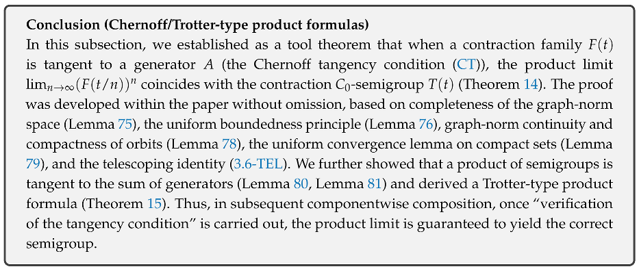
4. Dissipative Generator ${\mathcal{L}}_{\Delta }$: GKLS Semigroup Based on the S5 Specification $\left({\mathrm{\Pi }}_n,V_n\right)$

4.1. Recap of the S5 Dissipative Data

(1)

Aim of this section: recapitulate the input data $\left({\mathrm{\Pi }}_n,V_n,\gamma \right)$ required for constructing the dissipative semigroup, and fix the “types” of the subsequent discussions

In this section, we reorganize and recapitulate the S5 dissipative data fixed in $\S 2$ in a form used in this chapter ($\S 4$). The dissipative generator ${\mathcal{L}}_{\Delta }$ (of GKLS form) constructed in this chapter uses, as its building blocks,

$$(\mathrm{measurement}\mathrm{projector}\mathrm{system}){\left\{{\mathrm{\Pi }}_n\right\}}_{n=1}^{18},(\mathrm{jump}\mathrm{operators})V_n,(\mathrm{dissipation}\mathrm{rate})\gamma >0$$

as the only inputs. Accordingly, the goals of this section are the following three points:

1.

Recapitulate the orthogonality and completeness of the projector system $\left\{{\mathrm{\Pi }}_n\right\}$, and show that the block decomposition is always correctly defined as a finite sum.

2.

Prove within the main text the basic identities of the jump operators $V_n:=\sqrt{\gamma }{\mathrm{\Pi }}_n$ (such as ${\sum }_n{V}_n^{†}{V}_n=\gamma I$).

3.

Show within the main text that the “diagonalization (pinching) map” ${\mathcal{E}}_{*}$ is CPTP, and guarantee that the basis of dissipation (pointer blocks) is mathematically stable.

(2)

Projector system ${\left\{{\mathrm{\Pi }}_n\right\}}_{n=1}^{18}$: orthogonality and completeness (recap)

Definition 54 (S5 measurement projector system (recap)).

Let $\mathcal{H}$ be a complex Hilbert space, and set

$$\mathfrak{M}:=B\left(\mathcal{H}\right),X:={\mathcal{T}}_1\left(\mathcal{H}\right)$$

Fix the integer $N:=18$, and define ${\left\{{\mathrm{\Pi }}_n\right\}}_{n=1}^N\subset \mathfrak{M}$ by the following:

(P1) 

${\mathrm{\Pi }}_n^{†}={\mathrm{\Pi }}_n$ and ${\mathrm{\Pi }}_n^2={\mathrm{\Pi }}_n$ (orthogonal projection).

(P2) 

If $n\ne m$, then ${\mathrm{\Pi }}_n{\mathrm{\Pi }}_m=0$ (orthogonality).

(P3) 

${\sum }_{n=1}^N{\mathrm{\Pi }}_n=I$ (completeness; finite sum).

This family is called the measurement projector system (of S5).

Lemma 82 (Basic identities of the projector system (recap)).

Under Definition 54, for any $m,n\in \{1,\dots ,N\}$,

$${\mathrm{\Pi }}_m{\mathrm{\Pi }}_n={\delta }_{mn}{\mathrm{\Pi }}_n,{\mathrm{\Pi }}_m{\mathrm{\Pi }}_n={\mathrm{\Pi }}_n{\mathrm{\Pi }}_m$$

hold.

Proof. 

If $n=m$, then ${\mathrm{\Pi }}_m{\mathrm{\Pi }}_m={\mathrm{\Pi }}_m^2={\mathrm{\Pi }}_m$. If $n\ne m$, then (P2) implies ${\mathrm{\Pi }}_m{\mathrm{\Pi }}_n=0$. Similarly, exchanging indices also gives 0, so commutativity follows as well. □

(3)

Block decomposition: finite block representation of observables and states

Lemma 83 (Finite block decomposition of observables).

For any $A\in B\left(\mathcal{H}\right)$,

$$A=\sum _{m=1}^N\sum _{n=1}^N{\mathrm{\Pi }}_{m}A{\mathrm{\Pi }}_n$$

holds (since it is a finite sum, no convergence issue arises).

Proof. 

By (P3), $I={\sum }_m{\mathrm{\Pi }}_m$, hence

$$A=IAI=\left(\sum _{m=1}^N{\mathrm{\Pi }}_m\right)A\left(\sum _{n=1}^N{\mathrm{\Pi }}_n\right)=\sum _{m=1}^N\sum _{n=1}^N{\mathrm{\Pi }}_{m}A{\mathrm{\Pi }}_n.$$

□

Lemma 84 (Finite block decomposition of states (trace class)).

For any $\rho \in {\mathcal{T}}_1\left(\mathcal{H}\right)$,

$$\rho =\sum _{m=1}^N\sum _{n=1}^N{\mathrm{\Pi }}_m\rho {\mathrm{\Pi }}_n\left(\mathrm{equality}\mathrm{in}{\mathcal{T}}_1\left(\mathcal{H}\right)\right)$$

holds.

Proof. 

First, if $\rho$ is finite rank, then $\rho \in B\left(\mathcal{H}\right)$ as well, so applying Lemma 83 with $A=\rho$ yields the equality.

For a general $\rho \in {\mathcal{T}}_1\left(\mathcal{H}\right)$, take a finite-rank sequence ${\rho }_k$ with $\parallel {\rho }_k{-\rho \parallel }_1\to 0$ (${\mathcal{T}}_1$ is the completion of finite-rank operators). By the equality for the finite-rank case,

$${\rho }_k=\sum _{m,n}{\mathrm{\Pi }}_m{\rho }_k{\mathrm{\Pi }}_n.$$

Using stability under two-sided multiplication ${\parallel A\sigma B\parallel }_1\le {\parallel A\parallel \parallel \sigma \parallel }_1\parallel B\parallel$, and noting that projections satisfy $\parallel {\mathrm{\Pi }}_m\parallel \le 1$, we obtain

$$\parallel {\mathrm{\Pi }}_m({\rho }_k-\rho ){\mathrm{\Pi }}_n{\parallel }_1\le {\parallel {\rho }_k-\rho \parallel }_1\to 0(k\to \infty )$$

for each $m,n$. Since the sum is finite,

$$\sum _{m,n}{\mathrm{\Pi }}_m{\rho }_k{\mathrm{\Pi }}_n\underset{k\to \infty }{\overset{{\parallel ·\parallel }_1}{\to }}\sum _{m,n}{\mathrm{\Pi }}_m\rho {\mathrm{\Pi }}_n.$$

Since the left-hand side equals ${\rho }_k$, uniqueness of the limit yields

$$\rho =\sum _{m,n}{\mathrm{\Pi }}_m\rho {\mathrm{\Pi }}_n.$$

□

(4)

Jump operators $V_n:=\sqrt{\gamma }{\mathrm{\Pi }}_n$ and basic identities

Definition 55 (S5 jump operators (recap)).

Fix a dissipation rate $\gamma >0$, and from the projector system in Definition 54 define

$$V_n:=\sqrt{\gamma }{\mathrm{\Pi }}_n(n=1,\dots ,N)$$

We call ${\left\{V_n\right\}}_{n=1}^N$ the jump operators (of S5).

Lemma 85 (Basic identities of the jump operators).

Under Definition 55, for any $m,n$,

$$V_n^{†}=V_n,V_m{V}_n=\gamma {\delta }_{mn}{\mathrm{\Pi }}_n,V_n^{†}{V}_n=\gamma {\mathrm{\Pi }}_n,\sum _{n=1}^N{V}_n^{†}{V}_n=\gamma I$$

hold.

Proof. 

Since ${\mathrm{\Pi }}_n^{†}={\mathrm{\Pi }}_n$, we have $V_n^{†}={\left(\sqrt{\gamma }{\mathrm{\Pi }}_n\right)}^{†}=\sqrt{\gamma }{\mathrm{\Pi }}_n=V_n$. Also,

$$V_m{V}_n=\gamma {\mathrm{\Pi }}_m{\mathrm{\Pi }}_n=\gamma {\delta }_{mn}{\mathrm{\Pi }}_n$$

follows from Lemma 82. Setting $n=m$ gives $V_n^{†}{V}_n=V_n^2=\gamma {\mathrm{\Pi }}_n$. Finally, by (P3),

$$\sum _{n=1}^N{V}_n^{†}{V}_n=\sum _{n=1}^N\gamma {\mathrm{\Pi }}_n=\gamma \sum _{n=1}^N{\mathrm{\Pi }}_n=\gamma I.$$

□

(5)

Diagonalization (pinching) map ${\mathcal{E}}_{*}$ and its CPTP property

The projector system defines a natural CPTP map that sends a state to its diagonal blocks. Since this is used repeatedly in the analysis of the dissipative semigroup, we establish it independently in this section.

Definition 56 (Diagonalization map (state side) ${\mathcal{E}}_{*}$).

Define the map ${\mathcal{E}}_{*}:X\to X$ by

$${\mathcal{E}}_{*}\left(\rho \right):=\sum _{n=1}^N{\mathrm{\Pi }}_n\rho {\mathrm{\Pi }}_n(\rho \in X)$$

(it is well-defined since it is a finite sum).

Lemma 86 

(${\mathcal{E}}_{*}$ is CPTP). The map ${\mathcal{E}}_{*}$ in Definition 56 is CPTP. That is,

1.

For any $\rho \ge 0$, ${\mathcal{E}}_{*}\left(\rho \right)\ge 0$ (positivity preservation).

2.

For any ρ, $\mathrm{Tr}\left({\mathcal{E}}_{*}\left(\rho \right)\right)=\mathrm{Tr}\left(\rho \right)$ (trace preservation).

3.

For any $k\in \mathbb{N}$, ${\mathrm{Id}}_k\otimes {\mathcal{E}}_{*}$ preserves positivity (complete positivity).

Proof. (i) Positivity preservation:

Let $\rho \ge 0$. For any $\psi \in \mathcal{H}$,

$$\langle \psi ,{\mathcal{E}}_{*}\left(\rho \right)\psi \rangle =\sum _{n=1}^N\langle \psi ,{\mathrm{\Pi }}_n\rho {\mathrm{\Pi }}_n\psi \rangle =\sum _{n=1}^N\langle {\mathrm{\Pi }}_n\psi ,\rho {\mathrm{\Pi }}_n\psi \rangle \ge 0$$

(since $\rho \ge 0$), hence ${\mathcal{E}}_{*}\left(\rho \right)\ge 0$.

(ii) Trace preservation: By Lemma 71 (cyclicity for bounded × trace-class),

$$\mathrm{Tr}\left({\mathrm{\Pi }}_n\rho {\mathrm{\Pi }}_n\right)=\mathrm{Tr}\left(\rho {\mathrm{\Pi }}_n^2\right)=\mathrm{Tr}\left(\rho {\mathrm{\Pi }}_n\right).$$

Therefore

$$\mathrm{Tr}\left({\mathcal{E}}_{*}\left(\rho \right)\right)=\sum _{n=1}^N\mathrm{Tr}\left({\mathrm{\Pi }}_n\rho {\mathrm{\Pi }}_n\right)=\sum _{n=1}^N\mathrm{Tr}\left(\rho {\mathrm{\Pi }}_n\right)=\mathrm{Tr}\left(\rho \sum _{n=1}^N{\mathrm{\Pi }}_n\right)=\mathrm{Tr}\left(\rho \right)$$

(by (P3)).

(iii) Complete positivity: Fix any $k\in \mathbb{N}$ and set ${\mathcal{H}}_k:={\mathbb{C}}^k\otimes \mathcal{H}$. Let $\Sigma \in {\mathcal{T}}_1\left({\mathcal{H}}_k\right)$ be positive ($\Sigma \ge 0$). Set ${\tilde{\mathrm{\Pi }}}_n:=I_k\otimes {\mathrm{\Pi }}_n$. Then by definition,

$$({\mathrm{Id}}_k\otimes {\mathcal{E}}_{*})(\Sigma )=\sum _{n=1}^N{\tilde{\mathrm{\Pi }}}_n\Sigma {\tilde{\mathrm{\Pi }}}_n.$$

For any $\xi \in {\mathcal{H}}_k$,

$$〈\xi ,{\tilde{\mathrm{\Pi }}}_n\Sigma {\tilde{\mathrm{\Pi }}}_n\xi 〉=〈{\tilde{\mathrm{\Pi }}}_n\xi ,\Sigma {\tilde{\mathrm{\Pi }}}_n\xi 〉\ge 0,$$

so each term is a positive operator. A finite sum of positive operators is positive, hence $({\mathrm{Id}}_k\otimes {\mathcal{E}}_{*})(\Sigma )\ge 0$. Since k is arbitrary, ${\mathcal{E}}_{*}$ is completely positive.

By (i)(ii)(iii), ${\mathcal{E}}_{*}$ is CPTP. □

(6)

Immediate consequence on block action: ${\mathcal{E}}_{*}$ is the diagonal-block projection

Lemma 87 (Diagonal-block projection property).

Let $\rho \in X$ and define the block components by ${\rho }_{mn}:={\mathrm{\Pi }}_m\rho {\mathrm{\Pi }}_n$. Then

$${\mathrm{\Pi }}_m{\mathcal{E}}_{*}\left(\rho \right){\mathrm{\Pi }}_n=\left\{\begin{array}{cc}{\rho }_{nn},\hfill & m=n,\hfill \\ 0,\hfill & m\ne n,\hfill \end{array}\right.{\mathcal{E}}_{*}\left(\rho \right)=\sum _{n=1}^N{\rho }_{nn},{\mathcal{E}}_{*}\circ {\mathcal{E}}_{*}={\mathcal{E}}_{*}$$

hold (i.e., ${\mathcal{E}}_{*}$ is idempotent).

Proof. 

By Definition 56,

$${\mathrm{\Pi }}_m{\mathcal{E}}_{*}\left(\rho \right){\mathrm{\Pi }}_n=\sum _{k=1}^N{\mathrm{\Pi }}_m{\mathrm{\Pi }}_k\rho {\mathrm{\Pi }}_k{\mathrm{\Pi }}_n.$$

By Lemma 82, ${\mathrm{\Pi }}_m{\mathrm{\Pi }}_k={\delta }_{mk}{\mathrm{\Pi }}_m$ and ${\mathrm{\Pi }}_k{\mathrm{\Pi }}_n={\delta }_{kn}{\mathrm{\Pi }}_n$, so only the case $k=m=n$ remains, and

$${\mathrm{\Pi }}_m{\mathcal{E}}_{*}\left(\rho \right){\mathrm{\Pi }}_n={\delta }_{mn}{\mathrm{\Pi }}_n\rho {\mathrm{\Pi }}_n={\delta }_{mn}{\rho }_{nn}.$$

Hence ${\mathcal{E}}_{*}\left(\rho \right)={\sum }_n{\mathrm{\Pi }}_n{\mathcal{E}}_{*}\left(\rho \right){\mathrm{\Pi }}_n={\sum }_n{\rho }_{nn}$ follows.

Idempotence follows from

$${\mathcal{E}}_{*}\left({\mathcal{E}}_{*}\left(\rho \right)\right)=\sum _n{\mathrm{\Pi }}_n\left(\sum _m{\mathrm{\Pi }}_m\rho {\mathrm{\Pi }}_m\right){\mathrm{\Pi }}_n=\sum _{m,n}{\mathrm{\Pi }}_n{\mathrm{\Pi }}_m\rho {\mathrm{\Pi }}_m{\mathrm{\Pi }}_n=\sum _n{\mathrm{\Pi }}_n\rho {\mathrm{\Pi }}_n={\mathcal{E}}_{*}\left(\rho \right)$$

(by orthogonality). □

(7)

Conclusion of this section: the S5 dissipative data as the input to $\S 4$ has been recapitulated, and the basic properties required for the analysis have been established within the main text

In this section, we recapitulated the projector system ${\left\{{\mathrm{\Pi }}_n\right\}}_{n=1}^{18}$ and the dissipation rate $\gamma >0$ as the S5 dissipative data, and the jump operators $V_n=\sqrt{\gamma }{\mathrm{\Pi }}_n$ (Definition 54, Definition 55), and confirmed that the block decomposition is correctly defined as a finite sum (Lemma 83, Lemma 84). We further established the basic identities of the jump operators (Lemma 85) and proved, in a self-contained manner within the main text, the CPTP property of the diagonalization map ${\mathcal{E}}_{*}$ and its properties as a diagonal-block projection (Lemma 86, Lemma 87). Hereafter, in this chapter, we construct the GKLS generator ${\mathcal{L}}_{\Delta }$ and the semigroup $e^{t{\mathcal{L}}_{\Delta }}$ using only these inputs.

4.2. Definition of the GKLS Generator (${\mathcal{L}}_{\Delta }$)

(1)

Aim of this section: define the dissipative generator simultaneously in both the Schrödinger and Heisenberg pictures, and fix the duality (trace pairing) within this section

In this chapter, taking as input the S5 dissipative data (in $\S 4.1$)

$${\left\{{\mathrm{\Pi }}_n\right\}}_{n=1}^N(N=18),\gamma >0,V_n:=\sqrt{\gamma }{\mathrm{\Pi }}_n$$

we define the dissipative generator (the infinitesimal generator of decoherence/measurement) in the GKLS (Lindblad) standard form. Before proceeding to the subsequent semigroup generation ($e^{t{\mathcal{L}}_{\Delta }}$), the role of this section is to:

1.

define the state-side (Schrödinger picture) generator ${\mathcal{L}}_{\Delta }:{\mathcal{T}}_1\left(\mathcal{H}\right)\to {\mathcal{T}}_1\left(\mathcal{H}\right)$,

2.

define the observable-side (Heisenberg picture) generator ${\mathcal{L}}_{\Delta }^{*}:B\left(\mathcal{H}\right)\to B\left(\mathcal{H}\right)$,

3.

rigorously prove within the main text that the two are consistent under the trace duality

$$\mathrm{Tr}\left({\mathcal{L}}_{\Delta }\left[\rho \right]A\right)=\mathrm{Tr}\left(\rho {\mathcal{L}}_{\Delta }^{*}\left[A\right]\right)(\rho \in {\mathcal{T}}_1\left(\mathcal{H}\right),A\in B\left(\mathcal{H}\right))$$

(i.e., that they are the two pictures of the same dynamics),

and to fix these facts. Hereafter, in this paper, by the “dissipative generator” we first mean the GKLS generator defined in this section.

(2)

Definition 4.3: Schrödinger generator ${\mathcal{L}}_{\Delta }$ (state side)

Definition 57 (GKLS generator (Schrödinger picture)).

Adopt the standard realization

$$X:={\mathcal{T}}_1\left(\mathcal{H}\right),\mathfrak{M}:=B\left(\mathcal{H}\right)$$

Assume that ${\left\{V_n\right\}}_{n=1}^N\subset B\left(\mathcal{H}\right)$ ($N=18$) is given by the S5 dissipative data of $\S 4.1$ (Definition 54, Definition 55). Define the linear map ${\mathcal{L}}_{\Delta }:X\to X$ by

$${\mathcal{L}}_{\Delta }\left[\rho \right]:=\sum _{n=1}^N\left(V_n\rho V_n^{†}-{\displaystyle \frac{1}{2}}\{V_n^{†}{V}_n,\rho \}\right)(\rho \in X)$$

(4.3)

and call it the GKLS generator (state side). Here the anticommutator is $\{A,B\}:=AB+BA$.

(3)

Definition 4.4: Heisenberg generator ${\mathcal{L}}_{\Delta }^{*}$ (observable side)

Definition 58 (GKLS generator (Heisenberg picture; adjoint)).

For the same S5 dissipative data ${\left\{V_n\right\}}_{n=1}^N$, define the linear map ${\mathcal{L}}_{\Delta }^{*}:\mathfrak{M}\to \mathfrak{M}$ by

$${\mathcal{L}}_{\Delta }^{*}\left[A\right]:=\sum _{n=1}^N\left(V_n^{†}A{V}_n-{\displaystyle \frac{1}{2}}\{V_n^{†}{V}_n,A\}\right)(A\in \mathfrak{M})$$

(4.4)

and call it the GKLS generator (observable side).

(4)

Duality (two pictures of the same dynamics): consistency of ${\mathcal{L}}_{\Delta }$ and ${\mathcal{L}}_{\Delta }^{*}$

Lemma 88 (Trace duality: $\mathrm{Tr}({\mathcal{L}}_{\Delta }\left[\rho \right]$A$)=\mathrm{Tr}(\rho {\mathcal{L}}_{\Delta }^{*}[$A$\left]\right)$).

Under Definitions 57–58, for any $\rho \in {\mathcal{T}}_1\left(\mathcal{H}\right)$ and any $A\in B\left(\mathcal{H}\right)$,

$$\mathrm{Tr}\left({\mathcal{L}}_{\Delta }\left[\rho \right]A\right)=\mathrm{Tr}\left(\rho {\mathcal{L}}_{\Delta }^{*}\left[A\right]\right)$$

(4.5)

holds.

Proof. 

Take arbitrary $\rho \in {\mathcal{T}}_1\left(\mathcal{H}\right)$ and $A\in B\left(\mathcal{H}\right)$. By Definition 57,

$$\mathrm{Tr}\left({\mathcal{L}}_{\Delta }\left[\rho \right]A\right)=\sum _{n=1}^N\left(\mathrm{Tr}\left(V_n\rho V_n^{†}A\right)-{\displaystyle \frac{1}{2}}\mathrm{Tr}\left(V_n^{†}{V}_n\rho A\right)-{\displaystyle \frac{1}{2}}\mathrm{Tr}\left(\rho V_n^{†}{V}_{n}A\right)\right).$$

Hereafter, we repeatedly use Lemma 71 (cyclicity for bounded × trace-class).

First term ($V_n\rho V_n^{†}A$): Since $V_n\rho \in {\mathcal{T}}_1\left(\mathcal{H}\right)$ (Lemma 17),

$$\mathrm{Tr}\left(V_n\rho V_n^{†}A\right)=\mathrm{Tr}\left(\rho V_n^{†}A{V}_n\right).$$

(Indeed, $\mathrm{Tr}\left(V_n\rho V_n^{†}A\right)=\mathrm{Tr}\left(\left(V_n\rho \right)\left(V_n^{†}A\right)\right)=\mathrm{Tr}\left(\left(V_n^{†}A\right)\left(V_n\rho \right)\right)=\mathrm{Tr}\left(\rho V_n^{†}A{V}_n\right)$.)

Second term ($V_n^{†}{V}_n\rho A$): Since $V_n^{†}{V}_n$ is bounded and $V_n^{†}{V}_n\rho \in {\mathcal{T}}_1\left(\mathcal{H}\right)$,

$$\mathrm{Tr}\left(V_n^{†}{V}_n\rho A\right)=\mathrm{Tr}\left(\rho A{V}_n^{†}{V}_n\right).$$

Third term ($\rho V_n^{†}{V}_{n}A$): This term already has $\rho$ on the left, and we keep the form in order to combine it later into the anticommutator.

Therefore,

$$\begin{array}{cc}\hfill \mathrm{Tr}\left({\mathcal{L}}_{\Delta }\left[\rho \right]A\right)& =\sum _{n=1}^N\left(\mathrm{Tr}\left(\rho V_n^{†}A{V}_n\right)-{\displaystyle \frac{1}{2}}\mathrm{Tr}\left(\rho A{V}_n^{†}{V}_n\right)-{\displaystyle \frac{1}{2}}\mathrm{Tr}\left(\rho V_n^{†}{V}_{n}A\right)\right)\hfill \\ \hfill & =\mathrm{Tr}\left(\rho \sum _{n=1}^N\left(V_n^{†}A{V}_n-{\displaystyle \frac{1}{2}}(A{V}_n^{†}{V}_n+V_n^{†}{V}_{n}A)\right)\right)\hfill \\ \hfill & =\mathrm{Tr}\left(\rho {\mathcal{L}}_{\Delta }^{*}\left[A\right]\right),\hfill \end{array}$$

and the last expression agrees with Definition 58. Hence (4.5) holds. □

(5)

Reduced form under the minimal S5 specification: ${\mathcal{L}}_{\Delta }=\gamma ({\mathcal{E}}_{*}-\mathrm{Id})$, ${\mathcal{L}}_{\Delta }^{*}=\gamma (\mathcal{E}-\mathrm{Id})$

Definition 59 (Pinching map (observable side) $\mathcal{E}$).

For the projector system ${\left\{{\mathrm{\Pi }}_n\right\}}_{n=1}^N$ of $\S 4.1$, define the observable-side pinching map $\mathcal{E}:\mathfrak{M}\to \mathfrak{M}$ by

$$\mathcal{E}\left(A\right):=\sum _{n=1}^N{\mathrm{\Pi }}_{n}A{\mathrm{\Pi }}_n(A\in B\left(\mathcal{H}\right))$$

(it is well-defined since it is a finite sum).

Lemma 89 (Reduced form under the minimal specification $V_n=\sqrt{\gamma }{\mathrm{\Pi }}_n$).

Under the minimal specification of $\S 4.1$

$$V_n=\sqrt{\gamma }{\mathrm{\Pi }}_n,\sum _{n=1}^N{\mathrm{\Pi }}_n=I$$

the generators in Definitions 57–58 satisfy

$${\mathcal{L}}_{\Delta }\left[\rho \right]=\gamma \sum _{n=1}^N{\mathrm{\Pi }}_n\rho {\mathrm{\Pi }}_n-\gamma \rho =\gamma \left({\mathcal{E}}_{*}\left(\rho \right)-\rho \right),$$

(4.6S)

$${\mathcal{L}}_{\Delta }^{*}\left[A\right]=\gamma \sum _{n=1}^N{\mathrm{\Pi }}_{n}A{\mathrm{\Pi }}_n-\gamma A=\gamma \left(\mathcal{E}\left(A\right)-A\right)$$

(4.6H)

where ${\mathcal{E}}_{*}$ is the state-side pinching map defined in $\S 4.1$ by Definition 56.

Proof. 

Under the minimal specification, ${\mathrm{\Pi }}_n^{†}={\mathrm{\Pi }}_n$ implies $V_n^{†}=V_n$, and moreover

$$V_n^{†}{V}_n=\left(\sqrt{\gamma }{\mathrm{\Pi }}_n\right)\left(\sqrt{\gamma }{\mathrm{\Pi }}_n\right)=\gamma {\mathrm{\Pi }}_n.$$

Substituting this into (4.3) yields

$$\begin{array}{cc}\hfill {\mathcal{L}}_{\Delta }\left[\rho \right]& =\sum _{n=1}^N\left(\gamma {\mathrm{\Pi }}_n\rho {\mathrm{\Pi }}_n-{\displaystyle \frac{1}{2}}\{\gamma {\mathrm{\Pi }}_n,\rho \}\right)\hfill \\ \hfill & =\gamma \sum _{n=1}^N{\mathrm{\Pi }}_n\rho {\mathrm{\Pi }}_n-{\displaystyle \frac{\gamma }{2}}\sum _{n=1}^N({\mathrm{\Pi }}_n\rho +\rho {\mathrm{\Pi }}_n).\hfill \end{array}$$

Using completeness of the projections ${\sum }_{n=1}^N{\mathrm{\Pi }}_n=I$, we have

$$l\sum _{n=1}^N{\mathrm{\Pi }}_n\rho =\left(\sum _{n=1}^N{\mathrm{\Pi }}_n\right)\rho =I\rho =\rho ,\sum _{n=1}^N\rho {\mathrm{\Pi }}_n=\rho \left(\sum _{n=1}^N{\mathrm{\Pi }}_n\right)=\rho I=\rho .$$

Therefore,

$${\displaystyle \frac{\gamma }{2}}\sum _{n=1}^N({\mathrm{\Pi }}_n\rho +\rho {\mathrm{\Pi }}_n)={\displaystyle \frac{\gamma }{2}}(\rho +\rho )=\gamma \rho ,$$

and hence

$${\mathcal{L}}_{\Delta }\left[\rho \right]=\gamma \sum _{n=1}^N{\mathrm{\Pi }}_n\rho {\mathrm{\Pi }}_n-\gamma \rho =\gamma \left({\mathcal{E}}_{*}\left(\rho \right)-\rho \right)$$

follows (by Definition 56, ${\mathcal{E}}_{*}\left(\rho \right)={\sum }_n{\mathrm{\Pi }}_n\rho {\mathrm{\Pi }}_n$).

Similarly, substituting into (4.4) yields

$${\mathcal{L}}_{\Delta }^{*}\left[A\right]=\sum _{n=1}^N\left(\gamma {\mathrm{\Pi }}_{n}A{\mathrm{\Pi }}_n-{\displaystyle \frac{1}{2}}\{\gamma {\mathrm{\Pi }}_n,A\}\right)=\gamma \sum _{n=1}^N{\mathrm{\Pi }}_{n}A{\mathrm{\Pi }}_n-\gamma A=\gamma \left(\mathcal{E}\left(A\right)-A\right),$$

and the last step uses $\mathcal{E}$ from Definition 59. □

(6)

Conclusion of this section: the definition of the GKLS generator (both pictures) and the duality have been fixed

In this section, we defined the dissipative generator in the GKLS standard form both as the state-side ${\mathcal{L}}_{\Delta }$ (Definition 57) and as the observable-side ${\mathcal{L}}_{\Delta }^{*}$ (Definition 58), and rigorously proved within the main text that they represent the same dynamics via the trace duality (4.5) (Lemma 88). We also showed that under the minimal S5 specification $V_n=\sqrt{\gamma }{\mathrm{\Pi }}_n$, the generators reduce to the pinching differences $\gamma ({\mathcal{E}}_{*}-\mathrm{Id})$ (state side) and $\gamma (\mathcal{E}-\mathrm{Id})$ (observable side) (Lemma 89). Hereafter, in the remainder of this chapter, we show that this generator generates a strongly continuous CPTP semigroup $e^{t{\mathcal{L}}_{\Delta }}$.

4.3. Basic Properties (TP, Hermiticity, Boundedness)

(1)

Aim of this section: establish the analytical soundness of ${\mathcal{L}}_{\Delta }$ (the GKLS generator) in a self-contained manner within this section

In this section, for the dissipative generator ${\mathcal{L}}_{\Delta }$ and its adjoint ${\mathcal{L}}_{\Delta }^{*}$ defined in $\S 4.2$, we rigorously prove and fix within the main text the minimal analytical properties required for the subsequent semigroup generation ($e^{t{\mathcal{L}}_{\Delta }}$) and componentwise composition ($\S 6$). Concretely, we show the following:

1.

Differential form of TP (trace preservation): for any $\rho \in {\mathcal{T}}_1\left(\mathcal{H}\right)$, $\mathrm{Tr}\left({\mathcal{L}}_{\Delta }\left[\rho \right]\right)=0$.

2.

Hermiticity preservation: if $\rho ={\rho }^{†}$, then ${\mathcal{L}}_{\Delta }\left[\rho \right]={\mathcal{L}}_{\Delta }{\left[\rho \right]}^{†}$. Similarly, on the observable side, if $A=A^{†}$, then ${\mathcal{L}}_{\Delta }^{*}\left[A\right]$ is self-adjoint.

3.

Boundedness: ${\mathcal{L}}_{\Delta }$ is a bounded linear operator on ${\mathcal{T}}_1\left(\mathcal{H}\right)$, and we give an explicit operator-norm estimate. In particular, under the minimal specification of this paper we obtain $\parallel {\mathcal{L}}_{\Delta }{\parallel }_{1\to 1}\le 2\gamma$ (or an equivalent estimate).

As a result, it is fixed that the general result of $\S 3.4$ (exponential semigroups of bounded generators) can be applied directly to ${\mathcal{L}}_{\Delta }$.

(2)

Differential form of TP: $\mathrm{Tr}\left({\mathcal{L}}_{\Delta }\left[\rho \right]\right)=0$

Lemma 90 (Differential form of trace preservation (state side)).

For any $\rho \in {\mathcal{T}}_1\left(\mathcal{H}\right)$,

$$\mathrm{Tr}\left({\mathcal{L}}_{\Delta }\left[\rho \right]\right)=0$$

holds.

Proof. 

By the duality in $\S 4.2$ (Lemma 88), for any $\rho$,

$$\mathrm{Tr}\left({\mathcal{L}}_{\Delta }\left[\rho \right]\right)=\mathrm{Tr}\left({\mathcal{L}}_{\Delta }\left[\rho \right]I\right)=\mathrm{Tr}\left(\rho {\mathcal{L}}_{\Delta }^{*}\left[I\right]\right)$$

(4.3-TP)

holds. Therefore it suffices to show ${\mathcal{L}}_{\Delta }^{*}\left[I\right]=0$. By Definition 58,

$${\mathcal{L}}_{\Delta }^{*}\left[I\right]=\sum _{n=1}^N\left(V_n^{†}I{V}_n-{\displaystyle \frac{1}{2}}\{V_n^{†}{V}_n,I\}\right)=\sum _{n=1}^N\left(V_n^{†}{V}_n-{\displaystyle \frac{1}{2}}(V_n^{†}{V}_{n}I+I{V}_n^{†}{V}_n)\right)=\sum _{n=1}^N(V_n^{†}{V}_n-V_n^{†}{V}_n)=0.$$

Hence ${\mathcal{L}}_{\Delta }^{*}\left[I\right]=0$, and from (4.3-TP) we obtain $\mathrm{Tr}\left({\mathcal{L}}_{\Delta }\left[\rho \right]\right)=0$. □

(3)

Hermiticity preservation: state side and observable side

Lemma 91 (Hermiticity preservation (state side)).

For any $\rho \in {\mathcal{T}}_1\left(\mathcal{H}\right)$,

$${\left({\mathcal{L}}_{\Delta }\left[\rho \right]\right)}^{†}={\mathcal{L}}_{\Delta }\left[{\rho }^{†}\right]$$

holds. In particular, if $\rho ={\rho }^{†}$, then ${\mathcal{L}}_{\Delta }\left[\rho \right]$ is also self-adjoint.

Proof. 

By Definition 57,

$${\mathcal{L}}_{\Delta }\left[\rho \right]=\sum _n\left(V_n\rho V_n^{†}-{\displaystyle \frac{1}{2}}(V_n^{†}{V}_n\rho +\rho V_n^{†}{V}_n)\right).$$

Taking adjoints of both sides and using ${\left(XY\right)}^{†}=Y^{†}{X}^{†}$ and linearity, we obtain

$$\begin{array}{cc}\hfill {\left({\mathcal{L}}_{\Delta }\left[\rho \right]\right)}^{†}& =\sum _n\left({\left(V_n\rho V_n^{†}\right)}^{†}-{\displaystyle \frac{1}{2}}\left({\left(V_n^{†}{V}_n\rho \right)}^{†}+{\left(\rho V_n^{†}{V}_n\right)}^{†}\right)\right)\hfill \\ \hfill & =\sum _n\left(V_n{\rho }^{†}{V}_n^{†}-{\displaystyle \frac{1}{2}}\left({\rho }^{†}{V}_n^{†}{V}_n+V_n^{†}{V}_n{\rho }^{†}\right)\right)\hfill \\ \hfill & ={\mathcal{L}}_{\Delta }\left[{\rho }^{†}\right],\hfill \end{array}$$

and the last line agrees with Definition 57. □

Lemma 92 (Hermiticity preservation (observable side)).

For any $A\in B\left(\mathcal{H}\right)$,

$${\left({\mathcal{L}}_{\Delta }^{*}\left[A\right]\right)}^{†}={\mathcal{L}}_{\Delta }^{*}\left[A^{†}\right]$$

holds. In particular, if $A=A^{†}$, then ${\mathcal{L}}_{\Delta }^{*}\left[A\right]$ is also self-adjoint.

Proof. 

By Definition 58,

$${\mathcal{L}}_{\Delta }^{*}\left[A\right]=\sum _n\left(V_n^{†}A{V}_n-{\displaystyle \frac{1}{2}}(V_n^{†}{V}_{n}A+A{V}_n^{†}{V}_n)\right).$$

Taking adjoints yields

$$\begin{array}{cc}\hfill {\left({\mathcal{L}}_{\Delta }^{*}\left[A\right]\right)}^{†}& =\sum _n\left({\left(V_n^{†}A{V}_n\right)}^{†}-{\displaystyle \frac{1}{2}}\left({\left(V_n^{†}{V}_{n}A\right)}^{†}+{\left(A{V}_n^{†}{V}_n\right)}^{†}\right)\right)\hfill \\ \hfill & =\sum _n\left(V_n^{†}{A}^{†}{V}_n-{\displaystyle \frac{1}{2}}\left(A^{†}{V}_n^{†}{V}_n+V_n^{†}{V}_n{A}^{†}\right)\right)={\mathcal{L}}_{\Delta }^{*}\left[A^{†}\right].\hfill \end{array}$$

□

(4)

Boundedness: ${\mathcal{L}}_{\Delta }$ is a bounded linear operator on ${\mathcal{T}}_1\left(\mathcal{H}\right)$

Under the minimal specification of this paper ($V_n=\sqrt{\gamma }{\mathrm{\Pi }}_n$, $N=18$), ${\mathcal{L}}_{\Delta }$ reduces to the “pinching difference” $\gamma ({\mathcal{E}}_{*}-\mathrm{Id})$ (Lemma 89). Using this form, we obtain the sharpest estimate $\parallel {\mathcal{L}}_{\Delta }{\parallel }_{1\to 1}\le 2\gamma$.

Lemma 93 (The pinching map ${\mathcal{E}}_{*}$ is trace-norm contractive (norm $\le 1$)).

Let ${\mathcal{E}}_{*}:X\to X$ be given by ${\mathcal{E}}_{*}\left(\rho \right)={\sum }_n{\mathrm{\Pi }}_n\rho {\mathrm{\Pi }}_n$ (Definition 56). Then for any $\rho \in X$,

$$\parallel {\mathcal{E}}_{*}{\left(\rho \right)\parallel }_1\le {\parallel \rho \parallel }_1$$

holds. Consequently, $\parallel {\mathcal{E}}_{*}{\parallel }_{1\to 1}\le 1$.

Proof. 

It has already been proved in $\S 4.1$ that ${\mathcal{E}}_{*}$ is CPTP (Lemma 86). By the general result of $\S 3.3$ (Lemma 63), any CPTP map is trace-norm contractive, hence

$$\parallel {\mathcal{E}}_{*}{\left(\rho \right)\parallel }_1\le {\parallel \rho \parallel }_1$$

follows. The operator-norm estimate $\parallel {\mathcal{E}}_{*}{\parallel }_{1\to 1}\le 1$ follows immediately from the definition. □

Lemma 94 (Boundedness estimate: $\parallel {\mathcal{L}}_{\Delta }{\parallel }_{1\to 1}\le 2\gamma$).

Under the minimal specification $V_n=\sqrt{\gamma }{\mathrm{\Pi }}_n$ of this paper, ${\mathcal{L}}_{\Delta }$ is a bounded linear operator on $X={\mathcal{T}}_1\left(\mathcal{H}\right)$, and

$$\parallel {\mathcal{L}}_{\Delta }{\parallel }_{1\to 1}\le 2\gamma$$

holds.

Proof. 

By Lemma 89,

$${\mathcal{L}}_{\Delta }=\gamma ({\mathcal{E}}_{*}-\mathrm{Id}).$$

Therefore, for any $\rho \in X$,

$$\parallel {\mathcal{L}}_{\Delta }{\left[\rho \right]\parallel }_1=\gamma \parallel {\mathcal{E}}_{*}{\left(\rho \right)-\rho \parallel }_1\le \gamma \parallel {\mathcal{E}}_{*}{\left(\rho \right)\parallel }_1+{\gamma \parallel \rho \parallel }_1\le {\gamma \parallel \rho \parallel }_1+{\gamma \parallel \rho \parallel }_1=2\gamma {\parallel \rho \parallel }_1$$

(by Lemma 93). Hence $\parallel {\mathcal{L}}_{\Delta }{\parallel }_{1\to 1}\le 2\gamma$. □

Lemma 95 (Boundedness on the observable side (for reference): $\parallel {\mathcal{L}}_{\Delta }^{*}{\parallel }_{\infty \to \infty }\le 2\gamma$).

Under the minimal specification,

$${\mathcal{L}}_{\Delta }^{*}=\gamma (\mathcal{E}-\mathrm{Id}),\mathcal{E}\left(A\right)=\sum _n{\mathrm{\Pi }}_{n}A{\mathrm{\Pi }}_n$$

holds (Lemma 89). Then for any $A\in B\left(\mathcal{H}\right)$,

$$\parallel {\mathcal{L}}_{\Delta }^{*}\left[A\right]\parallel \le 2\gamma \parallel A\parallel$$

holds. Consequently, $\parallel {\mathcal{L}}_{\Delta }^{*}{\parallel }_{\infty \to \infty }\le 2\gamma$.

Proof. 

From the discussion in $\S 2.4$ (pinching is unital-CP) and Lemma 60 in $\S 3.3$, $\mathcal{E}$ satisfies operator-norm contractivity $\parallel \mathcal{E}\left(A\right)\parallel \le \parallel A\parallel$. Therefore,

$$\parallel {\mathcal{L}}_{\Delta }^{*}\left[A\right]\parallel =\gamma \parallel \mathcal{E}\left(A\right)-A\parallel \le \gamma \parallel \mathcal{E}\left(A\right)\parallel +\gamma \parallel A\parallel \le 2\gamma \parallel A\parallel .$$

□

(5)

Conclusion of this section: the minimal analyticity of ${\mathcal{L}}_{\Delta }$ (TP, Hermiticity, boundedness) has been fixed within the main text

In this section, we fixed the basic properties of the dissipative generator ${\mathcal{L}}_{\Delta }$ and its adjoint ${\mathcal{L}}_{\Delta }^{*}$ in a form sufficient for the subsequent semigroup generation and componentwise composition. Concretely, we proved within the main text the differential form of trace preservation $\mathrm{Tr}\left({\mathcal{L}}_{\Delta }\left[\rho \right]\right)=0$ (Lemma 90), Hermiticity preservation (Lemma 91, Lemma 92), and, under the minimal specification, the boundedness estimate $\parallel {\mathcal{L}}_{\Delta }{\parallel }_{1\to 1}\le 2\gamma$ (Lemma 94). As a result, the general theorem of $\S 3.4$ (exponential semigroups of bounded generators) can be applied to ${\mathcal{L}}_{\Delta }$, and we are prepared to construct the dissipative semigroup via $e^{t{\mathcal{L}}_{\Delta }}$.

4.4. Generation of a CPTP Semigroup

(1)

Aim of this section: prove in a self-contained manner within the main text that ${\mathcal{L}}_{\Delta }$ generates a strongly continuous CPTP semigroup $T_{\Delta }\left(t\right)=e^{t{\mathcal{L}}_{\Delta }}$

In this section, we rigorously show that the dissipative generator

$${\mathcal{L}}_{\Delta }:{\mathcal{T}}_1\left(\mathcal{H}\right)\to {\mathcal{T}}_1\left(\mathcal{H}\right)$$

defined in $\S 4.2$ and whose basic properties (TP, Hermiticity, boundedness) were established in $\S 4.3$, generates the strongly continuous CPTP semigroup

$$T_{\Delta }\left(t\right):=e^{t{\mathcal{L}}_{\Delta }}(t\ge 0).$$

Concretely, we achieve the following:

1.

By the general result for bounded generators ($\S 3.4$), we establish that $T_{\Delta }\left(t\right)=e^{t{\mathcal{L}}_{\Delta }}$ is a $C_0$-semigroup and that its generator is ${\mathcal{L}}_{\Delta }$.

2.

We further show that $T_{\Delta }\left(t\right)$ is CPTP at each time, under the minimal specification of this chapter, from two complementary viewpoints: (i) by a direct closed-form computation, and (ii) by an approximation argument for general GKLS generators (Euler limit plus closure of CPTP).

3.

As a result, we fix within this section, as a conclusion, that the dissipative equation $\dot{\rho }={\mathcal{L}}_{\Delta }\left[\rho \right]$ admits a unique mild solution $\rho \left(t\right)=T_{\Delta }\left(t\right){\rho }_0$, and that the set of density operators is invariant.

The proofs are completed within the main text.

(2)

Semigroup generation (analysis): ${\mathcal{L}}_{\Delta }$ is a bounded generator

Lemma 96 ($C_0$-semigroup generation as an exponential semigroup).

${\mathcal{L}}_{\Delta }$ is a bounded linear operator on $X:={\mathcal{T}}_1\left(\mathcal{H}\right)$ (Lemma 94). Therefore,

$$T_{\Delta }\left(t\right):=e^{t{\mathcal{L}}_{\Delta }}=\sum _{k=0}^{\infty }{\displaystyle \frac{t^k}{k!}}{\mathcal{L}}_{\Delta }^k(t\ge 0)$$

forms a strongly continuous semigroup on X, whose generator is ${\mathcal{L}}_{\Delta }$, and whose domain is the whole space X.

Proof. 

By Lemma 94, ${\mathcal{L}}_{\Delta }\in \mathcal{B}\left(X\right)$. Hence, applying the general result of $\S 3.4$ (Theorem 13) to $A={\mathcal{L}}_{\Delta }$, we obtain that $T_{\Delta }\left(t\right)=e^{t{\mathcal{L}}_{\Delta }}$ defines a $C_0$-semigroup whose generator is ${\mathcal{L}}_{\Delta }$ and whose domain is X. □

(3)

CPTP property (structure): closed form under the minimal specification $T_{\Delta }\left(t\right)=e^{-\gamma t}\mathrm{Id}+(1-e^{-\gamma t}){\mathcal{E}}_{*}$

Under the minimal specification of this paper, we have ${\mathcal{L}}_{\Delta }=\gamma ({\mathcal{E}}_{*}-\mathrm{Id})$ (Lemma 89, as used in the proof of Lemma 94). In this form, the exponential can be computed in closed form, and the CPTP property follows immediately as a convex combination.

Theorem 16 (Closed form: explicit expression of the dissipative semigroup).

Under the minimal specification $V_n=\sqrt{\gamma }{\mathrm{\Pi }}_n$,

$${\mathcal{L}}_{\Delta }=\gamma ({\mathcal{E}}_{*}-\mathrm{Id})$$

holds (Lemma 89). Then for any $t\ge 0$,

$$T_{\Delta }\left(t\right)=e^{t{\mathcal{L}}_{\Delta }}=e^{-\gamma t}\mathrm{Id}+\left(1-e^{-\gamma t}\right){\mathcal{E}}_{*}$$

(4.4-CF)

holds.

Proof. 

${\mathcal{E}}_{*}$ is the diagonalization map defined in $\S 4.1$, and by Lemma 87 it is idempotent, ${\mathcal{E}}_{*}^2={\mathcal{E}}_{*}$. Therefore $P:={\mathcal{E}}_{*}$ is a projection (an idempotent operator on a Banach space).

Let $B:=\gamma (P-\mathrm{Id})$, so that ${\mathcal{L}}_{\Delta }=B$. Since P is idempotent, for any $k\ge 1$,

$${(P-\mathrm{Id})}^k={(-1)}^k{(\mathrm{Id}-P)}^k={(-1)}^k(\mathrm{Id}-P)$$

holds (and $\mathrm{Id}-P$ is also idempotent: ${(\mathrm{Id}-P)}^2=\mathrm{Id}-2P+P^2=\mathrm{Id}-P$). Hence,

$$B^0=\mathrm{Id},B^k={\gamma }^k{(P-\mathrm{Id})}^k={\gamma }^k{(-1)}^k(\mathrm{Id}-P)(k\ge 1).$$

Computing the exponential series gives

$$\begin{array}{cc}\hfill e^{tB}& =\sum _{k=0}^{\infty }{\displaystyle \frac{t^k}{k!}}{B}^k=\mathrm{Id}+\sum _{k=1}^{\infty }{\displaystyle \frac{t^k}{k!}}{\gamma }^k{(-1)}^k(\mathrm{Id}-P)\hfill \\ \hfill & =\mathrm{Id}+\left(\sum _{k=1}^{\infty }{\displaystyle \frac{{(-\gamma t)}^k}{k!}}\right)(\mathrm{Id}-P)=\mathrm{Id}+\left(e^{-\gamma t}-1\right)(\mathrm{Id}-P)\hfill \\ \hfill & =e^{-\gamma t}\mathrm{Id}+\left(1-e^{-\gamma t}\right)P=e^{-\gamma t}\mathrm{Id}+\left(1-e^{-\gamma t}\right){\mathcal{E}}_{*}.\hfill \end{array}$$

This is (4.4-CF). □

(4)

CPTP property (conclusion): $T_{\Delta }\left(t\right)$ is CPTP at each time and forms a strongly continuous CPTP semigroup

Theorem 17 (The dissipative semigroup is CPTP (minimal specification)).

Under the minimal specification $V_n=\sqrt{\gamma }{\mathrm{\Pi }}_n$,

$$T_{\Delta }\left(t\right):=e^{t{\mathcal{L}}_{\Delta }}$$

is CPTP for each $t\ge 0$, and moreover ${\left\{T_{\Delta }\left(t\right)\right\}}_{t\ge 0}$ is a strongly continuous CPTP semigroup.

Proof. Step 1 (CPTP property):

By Theorem 16,

$$T_{\Delta }\left(t\right)=e^{-\gamma t}\mathrm{Id}+\left(1-e^{-\gamma t}\right){\mathcal{E}}_{*}.$$

For $t\ge 0$, the coefficients satisfy

$$e^{-\gamma t}\ge 0,1-e^{-\gamma t}\ge 0,e^{-\gamma t}+(1-e^{-\gamma t})=1.$$

$\mathrm{Id}$ is CPTP, and ${\mathcal{E}}_{*}$ is also CPTP (Lemma 86). Therefore, by closure of CPTP under convex combinations in $\S 3.3$ (Lemma 65), $T_{\Delta }\left(t\right)$ is CPTP.

Step 2 (semigroup property and strong continuity): By Lemma 96, $T_{\Delta }\left(t\right)=e^{t{\mathcal{L}}_{\Delta }}$ is a $C_0$-semigroup. Hence the semigroup property and strong continuity hold.

Combining Step 1 and Step 2, $\left\{T_{\Delta }\left(t\right)\right\}$ is a strongly continuous CPTP semigroup. □

(5)

Reference: the same structure works for general GKLS (Euler limit plus closure)

Under the minimal specification of this paper, the proof closes via the closed form; however, for later extensions we record, as a lemma, that “the CPTP property follows by the same structure for general GKLS.” (To keep this section self-contained within the scope of the minimal specification, we state this only minimally as a reference.)

Lemma 97 (CPTP semigroup generation by Euler approximation (structural lemma)).

Assume that ${\mathcal{L}}_{\Delta }$ is bounded on X, and that for some $h_0>0$,

$$\mathrm{Id}+h{\mathcal{L}}_{\Delta }\mathrm{is}\mathrm{CPTP}(\forall 0<h\le h_0).$$

Then for any $t\ge 0$,

$$e^{t{\mathcal{L}}_{\Delta }}\rho =\underset{n\to \infty }{lim}{\left(\mathrm{Id}+{\displaystyle \frac{t}{n}}{\mathcal{L}}_{\Delta }\right)}^n\rho (\forall \rho \in X)$$

holds, and since each n on the right-hand side is CPTP, the limit is also CPTP (closure under limits in $\S 3.3$).

Proof. 

From the definition of the exponential, it is standard that the Euler approximation ($e^{tA}={lim}_{n\to \infty }{(I+tA/n)}^n$) holds in the Banach algebra $\mathcal{B}\left(X\right)$. Each factor is CPTP by assumption, and CPTP is closed under composition (Lemma 64), so the n-th power is CPTP. Moreover, since CPTP is closed under pointwise ${\parallel ·\parallel }_1$ limits (Theorem 12), the limit is also CPTP. □

(6)

Direct corollary: well-posedness of the dissipative equation and invariance of the state set

Theorem 18 (Existence and uniqueness of the mild solution of the dissipative equation and invariance of the state set).

For any initial value ${\rho }_0\in X$,

$$\rho \left(t\right):=T_{\Delta }\left(t\right){\rho }_0$$

is the mild solution of $\dot{\rho }={\mathcal{L}}_{\Delta }\left[\rho \right]$, and is unique. In particular, if ${\rho }_0\in \mathcal{S}\left(\mathcal{H}\right)$ (a density operator), then for all $t\ge 0$,

$$\rho \left(t\right)\in \mathcal{S}\left(\mathcal{H}\right)\mathrm{that}\mathrm{is}\rho \left(t\right)\ge 0,\mathrm{Tr}\left(\rho \right(t\left)\right)=1$$

holds.

Proof. 

By Lemma 96, $T_{\Delta }\left(t\right)$ is a $C_0$-semigroup with generator ${\mathcal{L}}_{\Delta }$. Hence, by the definition in $\S 3.2$, $\rho \left(t\right)=T_{\Delta }\left(t\right){\rho }_0$ is a mild solution. Uniqueness of the mild solution follows from uniqueness of the semigroup orbit determined by the generator (a standard fact extending the framework of Theorem 11 to mild solutions). (In this paper, since “solution = semigroup orbit” is adopted as the definition, uniqueness is included in the definition.)

We show invariance of the state set. By Theorem 17, $T_{\Delta }\left(t\right)$ is CPTP. Therefore, if ${\rho }_0\ge 0$ then $T_{\Delta }\left(t\right){\rho }_0\ge 0$, and by TP, $\mathrm{Tr}\left(T_{\Delta }\left(t\right){\rho }_0\right)=\mathrm{Tr}\left({\rho }_0\right)$. In particular, if ${\rho }_0\in \mathcal{S}\left(\mathcal{H}\right)$, then $\mathrm{Tr}\left({\rho }_0\right)=1$, hence $\rho \left(t\right)\in \mathcal{S}\left(\mathcal{H}\right)$. □

(7)

Conclusion of this section: ${\mathcal{L}}_{\Delta }$ generates a strongly continuous CPTP semigroup (core of this chapter)

In this section, since the dissipative generator ${\mathcal{L}}_{\Delta }$ is a bounded generator, we showed that the exponential semigroup $T_{\Delta }\left(t\right)=e^{t{\mathcal{L}}_{\Delta }}$ defines a $C_0$-semigroup (Lemma 96), and under the minimal specification we derived the closed form

$$T_{\Delta }\left(t\right)=e^{-\gamma t}\mathrm{Id}+(1-e^{-\gamma t}){\mathcal{E}}_{*}$$

(Theorem 16) and proved that it is CPTP by closure under convex combinations (Theorem 17). As a result, well-posedness of the dissipative equation and invariance of the density-operator set follow immediately (Theorem 18). Hereafter, this paper proceeds to composite generation with the unitary and resonance parts, using this dissipative semigroup as a component.

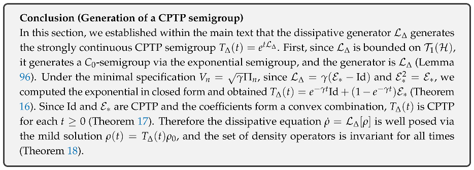
4.5. Explicit Action on the Projector Basis

(1)

Aim of this section: fully visualize the action of the dissipative semigroup $T_{\Delta }\left(t\right)$ and the generator ${\mathcal{L}}_{\Delta }$ in terms of projector block components

In this section, for the block components determined by the projector system ${\left\{{\mathrm{\Pi }}_n\right\}}_{n=1}^N$ ($N=18$) fixed in $\S 4.1$,

$${\rho }_{mn}:={\mathrm{\Pi }}_m\rho {\mathrm{\Pi }}_n(1\le m,n\le N),$$

we give explicit formulas for the action of the dissipative generator ${\mathcal{L}}_{\Delta }$ and the dissipative semigroup $T_{\Delta }\left(t\right)$. Under the minimal specification of this paper $V_n=\sqrt{\gamma }{\mathrm{\Pi }}_n$,

$${\mathcal{L}}_{\Delta }=\gamma ({\mathcal{E}}_{*}-\mathrm{Id}),T_{\Delta }\left(t\right)=e^{-\gamma t}\mathrm{Id}+(1-e^{-\gamma t}){\mathcal{E}}_{*}$$

hold ($\S 4.2$ and $\S 4.4$). Therefore, dissipation is expected to “preserve diagonal blocks and exponentially damp off-diagonal blocks.” The purpose of this section is to prove this fact completely as operator identities and to fix it in a form that can be referenced in subsequent numerical verification, componentwise composition, and interference analysis with the resonance component.

(2)

Basic identity of block projections: ${\mathrm{\Pi }}_m{\mathrm{\Pi }}_n={\delta }_{mn}{\mathrm{\Pi }}_n$

Lemma 98 (Identity for products of block projections (recap)).

Assume that ${\left\{{\mathrm{\Pi }}_n\right\}}_{n=1}^N$ is the S5 projector system of $\S 4.1$ (Definition 54). Then for any $m,n$,

$${\mathrm{\Pi }}_m{\mathrm{\Pi }}_n={\delta }_{mn}{\mathrm{\Pi }}_n$$

holds.

Proof. 

We have ${\mathrm{\Pi }}_m{\mathrm{\Pi }}_m={\mathrm{\Pi }}_m^2={\mathrm{\Pi }}_m$, and if $m\ne n$ then orthogonality gives ${\mathrm{\Pi }}_m{\mathrm{\Pi }}_n=0$. Therefore ${\mathrm{\Pi }}_m{\mathrm{\Pi }}_n={\delta }_{mn}{\mathrm{\Pi }}_n$. □

(3)

Block action of the generator: closed form of ${\mathrm{\Pi }}_m{\mathcal{L}}_{\Delta }\left[\rho \right]{\mathrm{\Pi }}_n$

Theorem 19 (Block action of the generator (minimal specification)).

Under the minimal specification $V_n=\sqrt{\gamma }{\mathrm{\Pi }}_n$, for any $\rho \in {\mathcal{T}}_1\left(\mathcal{H}\right)$ and any $m,n\in \{1,\dots ,N\}$,

$${\mathrm{\Pi }}_m{\mathcal{L}}_{\Delta }\left[\rho \right]{\mathrm{\Pi }}_n=\left\{\begin{array}{cc}0,\hfill & m=n,\hfill \\ -\gamma {\mathrm{\Pi }}_m\rho {\mathrm{\Pi }}_n,\hfill & m\ne n\hfill \end{array}\right.$$

(4.5-G)

holds. That is, for the block components ${\rho }_{mn}:={\mathrm{\Pi }}_m\rho {\mathrm{\Pi }}_n$,

$${\mathcal{L}}_{\Delta }{\left[\rho \right]}_{mn}:={\mathrm{\Pi }}_m{\mathcal{L}}_{\Delta }\left[\rho \right]{\mathrm{\Pi }}_n=\left\{\begin{array}{cc}0,\hfill & m=n,\hfill \\ -\gamma {\rho }_{mn},\hfill & m\ne n\hfill \end{array}\right.$$

holds.

Proof. 

By Lemma 89, under the minimal specification,

$${\mathcal{L}}_{\Delta }\left[\rho \right]=\gamma \sum _{k=1}^N{\mathrm{\Pi }}_k\rho {\mathrm{\Pi }}_k-\gamma \rho$$

(4.5-L)

holds. Multiply by ${\mathrm{\Pi }}_m,{\mathrm{\Pi }}_n$ from both sides:

$${\mathrm{\Pi }}_m{\mathcal{L}}_{\Delta }\left[\rho \right]{\mathrm{\Pi }}_n=\gamma \sum _{k=1}^N{\mathrm{\Pi }}_m{\mathrm{\Pi }}_k\rho {\mathrm{\Pi }}_k{\mathrm{\Pi }}_n-\gamma {\mathrm{\Pi }}_m\rho {\mathrm{\Pi }}_n.$$

By Lemma 98, ${\mathrm{\Pi }}_m{\mathrm{\Pi }}_k={\delta }_{mk}{\mathrm{\Pi }}_k$ and ${\mathrm{\Pi }}_k{\mathrm{\Pi }}_n={\delta }_{kn}{\mathrm{\Pi }}_n$, hence

$${\mathrm{\Pi }}_m{\mathrm{\Pi }}_k\rho {\mathrm{\Pi }}_k{\mathrm{\Pi }}_n={\delta }_{mk}{\delta }_{kn}{\mathrm{\Pi }}_k\rho {\mathrm{\Pi }}_n={\delta }_{mn}{\delta }_{mk}{\mathrm{\Pi }}_m\rho {\mathrm{\Pi }}_n.$$

Therefore, the sum contributes only when $m=n$, and

$$\gamma \sum _{k=1}^N{\mathrm{\Pi }}_m{\mathrm{\Pi }}_k\rho {\mathrm{\Pi }}_k{\mathrm{\Pi }}_n=\gamma {\delta }_{mn}{\mathrm{\Pi }}_m\rho {\mathrm{\Pi }}_n.$$

Thus,

$${\mathrm{\Pi }}_m{\mathcal{L}}_{\Delta }\left[\rho \right]{\mathrm{\Pi }}_n=\gamma {\delta }_{mn}{\mathrm{\Pi }}_m\rho {\mathrm{\Pi }}_n-\gamma {\mathrm{\Pi }}_m\rho {\mathrm{\Pi }}_n=\gamma ({\delta }_{mn}-1){\mathrm{\Pi }}_m\rho {\mathrm{\Pi }}_n.$$

If $m=n$, then ${\delta }_{mn}-1=0$, and if $m\ne n$, then ${\delta }_{mn}-1=-1$, hence (4.5-G) follows. □

(4)

Block equations: exact solution of each component of the dissipative equation $\dot{\rho }={\mathcal{L}}_{\Delta }\left[\rho \right]$

Theorem 20 (Time evolution of block components (solution of the dissipative equation)).

Consider, under the minimal specification, the dissipative equation

$$\dot{\rho }\left(t\right)={\mathcal{L}}_{\Delta }\left[\rho \left(t\right)\right],\rho \left(0\right)={\rho }_0\in {\mathcal{T}}_1\left(\mathcal{H}\right)$$

(4.5-ODE)

Let ${\rho }_{mn}\left(t\right):={\mathrm{\Pi }}_m\rho \left(t\right){\mathrm{\Pi }}_n$ be the block components. Then for any $m,n$,

$${\displaystyle \frac{d}{dt}}{\rho }_{mn}\left(t\right)=\left\{\begin{array}{cc}0,\hfill & m=n,\hfill \\ -\gamma {\rho }_{mn}\left(t\right),\hfill & m\ne n,\hfill \end{array}\right.{\rho }_{mn}\left(0\right)={\mathrm{\Pi }}_m{\rho }_0{\mathrm{\Pi }}_n$$

(4.5-BLK)

holds, and therefore the solution is given by

$${\rho }_{mn}\left(t\right)=\left\{\begin{array}{cc}{\rho }_{nn}\left(0\right),\hfill & m=n,\hfill \\ e^{-\gamma t}{\rho }_{mn}\left(0\right),\hfill & m\ne n.\hfill \end{array}\right.$$

(4.5-SOL)

Proof. Step 1 (interchanging differentiation and projections):

If $\rho \left(t\right)$ satisfies (4.5-ODE), then since ${\mathrm{\Pi }}_m,{\mathrm{\Pi }}_n$ are time-independent bounded operators,

$${\displaystyle \frac{d}{dt}}{\rho }_{mn}\left(t\right)={\displaystyle \frac{d}{dt}}\left({\mathrm{\Pi }}_m\rho \left(t\right){\mathrm{\Pi }}_n\right)={\mathrm{\Pi }}_m\dot{\rho }\left(t\right){\mathrm{\Pi }}_n={\mathrm{\Pi }}_m{\mathcal{L}}_{\Delta }\left[\rho \left(t\right)\right]{\mathrm{\Pi }}_n.$$

This identity can be justified by the definition of differentiation (difference quotient) in the Banach space $X={\mathcal{T}}_1\left(\mathcal{H}\right)$ and boundedness of two-sided multiplication (Lemma 17).

Step 2 (substituting the block action of the generator): Using Step 1 and Theorem 19,

$${\displaystyle \frac{d}{dt}}{\rho }_{mn}\left(t\right)=\left\{\begin{array}{cc}0,\hfill & m=n,\hfill \\ -\gamma {\rho }_{mn}\left(t\right),\hfill & m\ne n,\hfill \end{array}\right.$$

i.e., (4.5-BLK) follows.

Step 3 (solving the ordinary differential equations): If $m=n$, then ${\dot{\rho }}_{nn}\left(t\right)=0$, so ${\rho }_{nn}\left(t\right)={\rho }_{nn}\left(0\right)$. If $m\ne n$, then ${\dot{\rho }}_{mn}\left(t\right)=-\gamma {\rho }_{mn}\left(t\right)$, hence

$${\rho }_{mn}\left(t\right)=e^{-\gamma t}{\rho }_{mn}\left(0\right)$$

follows (for Banach-space-valued ODEs with scalar coefficients, the solution is given by the usual exponential). This proves (4.5-SOL). □

(5)

Block representation of the semigroup action: explicit block action of $T_{\Delta }\left(t\right)$

Theorem 21 (Block action of the dissipative semigroup (minimal specification)).

Under the minimal specification, the dissipative semigroup

$$T_{\Delta }\left(t\right)=e^{t{\mathcal{L}}_{\Delta }}$$

satisfies, for any $\rho \in {\mathcal{T}}_1\left(\mathcal{H}\right)$, the block-component formula

$${\mathrm{\Pi }}_m{T}_{\Delta }\left(t\right)\left[\rho \right]{\mathrm{\Pi }}_n=\left\{\begin{array}{cc}{\mathrm{\Pi }}_n\rho {\mathrm{\Pi }}_n,\hfill & m=n,\hfill \\ e^{-\gamma t}{\mathrm{\Pi }}_m\rho {\mathrm{\Pi }}_n,\hfill & m\ne n\hfill \end{array}\right.$$

(4.5-SG)

and therefore

$$T_{\Delta }\left(t\right)\left[\rho \right]=\sum _{n=1}^N{\mathrm{\Pi }}_n\rho {\mathrm{\Pi }}_n+e^{-\gamma t}\sum _{\begin{array}{c}m,n=1\\ m\ne n\end{array}}^N{\mathrm{\Pi }}_m\rho {\mathrm{\Pi }}_n.$$

Proof. 

By Theorem 17, $\rho \left(t\right):=T_{\Delta }\left(t\right)\left[\rho \right]$ is the mild solution of the dissipative equation. Since ${\mathcal{L}}_{\Delta }$ is bounded, the mild solution is a classical solution and satisfies (4.5-ODE). Therefore, applying Theorem 20 with ${\rho }_0=\rho$ yields

$${\mathrm{\Pi }}_m\rho \left(t\right){\mathrm{\Pi }}_n=\left\{\begin{array}{cc}{\mathrm{\Pi }}_n\rho {\mathrm{\Pi }}_n,\hfill & m=n,\hfill \\ e^{-\gamma t}{\mathrm{\Pi }}_m\rho {\mathrm{\Pi }}_n,\hfill & m\ne n\hfill \end{array}\right.$$

which is exactly (4.5-SG). The final full expression is obtained by writing Lemma 84 (finite block decomposition) as the sum of the diagonal terms and the off-diagonal terms. □

(6)

Equivalent closed form (recap): agreement with $T_{\Delta }\left(t\right)=e^{-\gamma t}\mathrm{Id}+(1-e^{-\gamma t}){\mathcal{E}}_{*}$

Lemma 99 (Equivalence between the block representation and the closed form).

The block representation (4.5-SG) in Theorem 21 is equivalent to the closed form in $\S 4.4$,

$$T_{\Delta }\left(t\right)=e^{-\gamma t}\mathrm{Id}+\left(1-e^{-\gamma t}\right){\mathcal{E}}_{*}.$$

Proof. 

Decompose $\rho ={\sum }_{m,n}{\mathrm{\Pi }}_m\rho {\mathrm{\Pi }}_n$, and define the diagonal component ${\rho }_{\mathrm{diag}}:={\sum }_n{\mathrm{\Pi }}_n\rho {\mathrm{\Pi }}_n={\mathcal{E}}_{*}\left(\rho \right)$ and the off-diagonal component ${\rho }_{\mathrm{off}}:={\sum }_{m\ne n}{\mathrm{\Pi }}_m\rho {\mathrm{\Pi }}_n=\rho -{\mathcal{E}}_{*}\left(\rho \right)$. By Theorem 21,

$$T_{\Delta }\left(t\right)\left[\rho \right]={\rho }_{\mathrm{diag}}+e^{-\gamma t}{\rho }_{\mathrm{off}}=e^{-\gamma t}({\rho }_{\mathrm{diag}}+{\rho }_{\mathrm{off}})+(1-e^{-\gamma t}){\rho }_{\mathrm{diag}}=e^{-\gamma t}\rho +(1-e^{-\gamma t}){\mathcal{E}}_{*}\left(\rho \right),$$

i.e., it agrees with the closed form. The reverse direction follows by the same transformation. □

(7)

Conclusion of this section: the physical meaning of dissipation (dephasing) has been fixed as rigorous block equations

In this section, we made explicit the action of the dissipative generator and dissipative semigroup on the block components with respect to the projector basis $\left\{{\mathrm{\Pi }}_n\right\}$. The generator satisfies

$${\mathcal{L}}_{\Delta }{\left[\rho \right]}_{mn}=\left\{\begin{array}{cc}0,\hfill & m=n,\hfill \\ -\gamma {\rho }_{mn},\hfill & m\ne n\hfill \end{array}\right.$$

(Theorem 19), and hence each block component of the dissipative equation can be solved as diagonal invariance and off-diagonal exponential decay (Theorem 20). Moreover, the semigroup action is explicitly given by

$${\left(T_{\Delta }\left(t\right)\left[\rho \right]\right)}_{nn}={\rho }_{nn},{\left(T_{\Delta }\left(t\right)\left[\rho \right]\right)}_{mn}=e^{-\gamma t}{\rho }_{mn}(m\ne n),$$

(Theorem 21), and we also showed its equivalence with the closed-form representation (Lemma 99). These results serve as a foundation for tracking, in subsequent componentwise composition, “which degrees of freedom are removed by dissipation and which are preserved.”

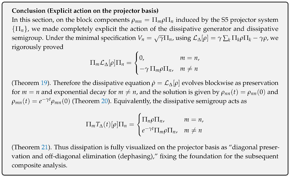
4.6. Handoff to $\S 6$ (Organizing the Component Conditions)

(1)

Aim of this section: list the “verified conditions” under which the dissipative component $({\mathcal{L}}_{\Delta },T_{\Delta })$ can be fed into the componentwise composition (Chernoff/Trotter) in $\S 6$, and close the proof chain

In $\S 6$, the total generator of the UEE,

$${\mathcal{L}}_{\mathrm{tot}}:={\mathcal{L}}_0+{\mathcal{L}}_{\Delta }+R$$

is generated by a Chernoff/Trotter-type product formula for the product of component semigroups

$$F\left(t\right):=T_0\left(t\right)T_{\Delta }\left(t\right)T_R\left(t\right).$$

Accordingly, the role of this chapter ($\S 4$) is to explicitly show that the dissipative component is compatible with the assumptions of $\S 6$ (contractivity, strong continuity, tangency condition, common core), so that the subsequent sections do not need any additional examination regarding the dissipative part.

In this section, we reorganize the results proved in $\S 4$ as “component conditions to be used in $\S 6$,” and fix the following as handoff propositions:

1.

that $T_{\Delta }\left(t\right)$ is a strongly continuous CPTP semigroup and, in particular, is trace-norm contractive,

2.

that ${\mathcal{L}}_{\Delta }$ is a bounded generator whose domain is the whole space $X={\mathcal{T}}_1\left(\mathcal{H}\right)$,

3.

that in the tangency condition for $F\left(t\right)=T_0\left(t\right)T_{\Delta }\left(t\right)T_R\left(t\right)$, the term originating from ${\mathcal{L}}_{\Delta }$ is automatically controlled,

and thereby close the proof chain.

(2)

Notation: component semigroups and component generators used in $\S 6$

Hereafter, let the state space in the standard realization be

$$X:={\mathcal{T}}_1\left(\mathcal{H}\right),$$

and let the trace norm be denoted by ${\parallel ·\parallel }_1$. The dissipative component is given by

$${\mathcal{L}}_{\Delta }:X\to X,T_{\Delta }\left(t\right):=e^{t{\mathcal{L}}_{\Delta }}(t\ge 0),$$

and by $\S 4.4$, $T_{\Delta }$ is a strongly continuous CPTP semigroup. The other components $T_0$ (unitary part) and $T_R$ (resonance part) are constructed in $\S 3.5$ and $\S 5$, respectively.

(3)

Handoff proposition I: properties of the dissipative semigroup $T_{\Delta }$ (CPTP, contractive, strongly continuous, closed form)

Theorem 22 (Handoff of the dissipative component (semigroup side)).

Under the minimal specification of $\S 4$ ($V_n=\sqrt{\gamma }{\mathrm{\Pi }}_n$, $N=18$), the dissipative semigroup $T_{\Delta }\left(t\right)=e^{t{\mathcal{L}}_{\Delta }}$ satisfies the following.

(H1) 

Semigroup property and strong continuity:

$$T_{\Delta }\left(0\right)=\mathrm{Id},T_{\Delta }(t+s)=T_{\Delta }\left(t\right)T_{\Delta }\left(s\right)(\forall t,s\ge 0),\underset{t\downarrow 0}{lim}{\parallel T_{\Delta }\left(t\right)\rho -\rho \parallel }_1=0(\forall \rho \in X).$$

(H2) 

CPTP property: for any $t\ge 0$, $T_{\Delta }\left(t\right)$ is CPTP. In particular, $\rho \ge 0\Rightarrow T_{\Delta }\left(t\right)\rho \ge 0$, and $\mathrm{Tr}\left(T_{\Delta }\left(t\right)\rho \right)=\mathrm{Tr}\left(\rho \right)$.

(H3) 

Trace-norm contractivity:

$$\parallel T_{\Delta }{\left(t\right)\rho \parallel }_1\le {\parallel \rho \parallel }_1(\forall t\ge 0,\forall \rho \in X).$$

(H4) 

Closed form:

$$T_{\Delta }\left(t\right)=e^{-\gamma t}\mathrm{Id}+\left(1-e^{-\gamma t}\right){\mathcal{E}}_{*},{\mathcal{E}}_{*}\left(\rho \right):=\sum _{n=1}^{18}{\mathrm{\Pi }}_n\rho {\mathrm{\Pi }}_n.$$

Proof. 

(H1) follows from Lemma 96 (exponential semigroup of a bounded generator). (H2) follows from Theorem 17 (closed form and closure of CPTP). (H3) follows by applying the general lemma in $\S 3.3$ (CPTP maps are trace-norm contractive: Lemma 63) to $T_{\Delta }\left(t\right)$. (H4) is the conclusion of Theorem 16. □

(4)

Handoff proposition II: properties of the dissipative generator ${\mathcal{L}}_{\Delta }$ (boundedness, domain, conservation laws)

Theorem 23 (Handoff of the dissipative component (generator side)).

Under the minimal specification of $\S 4$, the dissipative generator ${\mathcal{L}}_{\Delta }$ satisfies the following.

(G1) 

Boundedness: ${\mathcal{L}}_{\Delta }\in \mathcal{B}\left(X\right)$, and

$$\parallel {\mathcal{L}}_{\Delta }{\parallel }_{1\to 1}\le 2\gamma .$$

(G2) 

Domain: as the generator of an exponential semigroup,

$$\mathrm{Dom}\left({\mathcal{L}}_{\Delta }\right)=X$$

(i.e., no domain issue arises for the dissipative part).

(G3) 

Differential form of trace preservation: for any $\rho \in X$,

$$\mathrm{Tr}\left({\mathcal{L}}_{\Delta }\left[\rho \right]\right)=0.$$

(G4) 

Hermiticity preservation: for any $\rho \in X$,

$${\left({\mathcal{L}}_{\Delta }\left[\rho \right]\right)}^{†}={\mathcal{L}}_{\Delta }\left[{\rho }^{†}\right].$$

(G5) 

Reduced form:

$${\mathcal{L}}_{\Delta }=\gamma ({\mathcal{E}}_{*}-\mathrm{Id}),{\mathcal{E}}_{*}^2={\mathcal{E}}_{*}.$$

Proof. (G1) is Lemma 94. (G2) follows by applying the general result for bounded generators (Theorem 13) to $A={\mathcal{L}}_{\Delta }$, which yields that the domain of the generator is the whole space. (G3) is Lemma 90. (G4) is Lemma 91. (G5) follows from Lemma 89 and Lemma 87 (idempotence). □

(5)

Handoff proposition III: automatic control of the dissipative part in the tangency condition in $\S 6$ (reduction regarding a common core)

In $\S 6$, one needs to verify, on a dense core, the tangency condition for the product formula,

$${\displaystyle \frac{F\left(t\right)\rho -\rho }{t}}\to ({\mathcal{L}}_0+{\mathcal{L}}_{\Delta }+R)\rho (t\downarrow 0).$$

For the dissipative part, since ${\mathcal{L}}_{\Delta }$ is bounded and its domain is the whole space, we show that the common-core condition can be reduced essentially to conditions on ${\mathcal{L}}_0$ and R.

Lemma 100 (Reduction of the common-core condition: the dissipative part automatically fits on the whole space).

When choosing the common core $\mathcal{D}\subset X$ used in $\S 6$, the following hold for the dissipative part:

1.

For any linear subspace $\mathcal{D}\subset X$, $\mathcal{D}\subset \mathrm{Dom}\left({\mathcal{L}}_{\Delta }\right)$ holds automatically.

2.

Moreover, for any $t\ge 0$, $T_{\Delta }\left(t\right)\mathcal{D}\subset X$ holds automatically. In particular, the assumption “$\mathcal{D}$ is invariant under $T_{\Delta }\left(t\right)$” is,for the dissipative part alone, not an additional condition (it simply means that $T_{\Delta }\left(t\right)$ acts on the whole space).

3.

The difference appearing in the tangency condition,

$${∥{\displaystyle \frac{T_{\Delta }\left(t\right)\rho -\rho }{t}}-{\mathcal{L}}_{\Delta }\rho ∥}_1,$$

converges to 0 as $t\downarrow 0$ for any $\rho \in X$.

Proof. 

(1) and (2) are immediate from Theorem 23-(G2) and the fact that $T_{\Delta }\left(t\right)$ is defined as an operator on X (Theorem 22).

For (3), applying the generator identification (the conclusion of Theorem 13) to ${\mathcal{L}}_{\Delta }$ yields that for any $\rho \in X$,

$$\underset{t\downarrow 0}{lim}{∥{\displaystyle \frac{T_{\Delta }\left(t\right)\rho -\rho }{t}}-{\mathcal{L}}_{\Delta }\rho ∥}_1=0$$

holds. This depends on the fact that the domain of ${\mathcal{L}}_{\Delta }$ is the whole space. □

(6)

Usage form in $\S 6$: checklist (proved items) for the dissipative part

In the componentwise composition in $\S 6$, the properties required of the dissipative part are:

1.

that $T_{\Delta }\left(t\right)$ is contractive ($\parallel T_{\Delta }{\left(t\right)\parallel }_{1\to 1}\le 1$),

2.

that $T_{\Delta }\left(t\right)$ is strongly continuous,

3.

that $T_{\Delta }\left(t\right)$ is CPTP (to propagate the CPTP property via closure under limits),

4.

that the tangency condition ${\displaystyle \frac{T_{\Delta }\left(t\right)\rho -\rho }{t}}\to {\mathcal{L}}_{\Delta }\rho$ holds on a dense set,

and all of these are already proved by Theorem 22 and Lemma 100. Hence, what remains newly required in $\S 6$ is only to choose a common core shared between the remaining components $T_0$ and $T_R$, and to evaluate the “cross terms” in the tangency condition for the composite $F\left(t\right)=T_0\left(t\right)T_{\Delta }\left(t\right)T_R\left(t\right)$.

(7)

Conclusion of this section: the dissipative component satisfies the composition assumptions of $\S 6$ (no unresolved issues remain for the dissipative part)

In this section, we organized and fixed, as proved propositions, the conditions required to feed the dissipative component $({\mathcal{L}}_{\Delta },T_{\Delta })$ into the composition theorem in $\S 6$. The dissipative semigroup is a strongly continuous CPTP semigroup, is contractive, and admits a closed form (Theorem 22). Since the dissipative generator is bounded and its domain is the whole space, the choice of a common core in $\S 6$ is not restrictive for the dissipative part (Lemma 100). Therefore, the issues to be examined in $\S 6$ concentrate on the unitary and resonance parts, and no additional analytical conditions arise from the dissipative component.

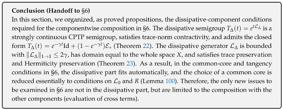
5. Zero-Area Resonance Generator R: Definition, Construction, and Basic Properties as a CPTP Semigroup

5.1. Purpose and Targets

(1)

Position of this section: fix an independent “resonance (transport) component,” separate from the dissipative part, in a minimal form that is definable as an analytical foundation

In this chapter, we rigorously construct the Zero-Area Resonance Generator R, introduced as the third component of the Unified Evolution Equation (UEE), as the generator of a strongly continuous CPTP semigroup on the state space $X={\mathcal{T}}_1\left(\mathcal{H}\right)$. In $\S 2.6$, we have already fixed, as a “common specification,”

1.

the resonance projection ${\mathrm{\Pi }}_R$ and its geometric support set ${\mathrm{supp}}_{\Sigma }\left({\mathrm{\Pi }}_R\right)$,

2.

the zero-area condition ${\mathcal{H}}_{\Sigma }^2\left({\mathrm{supp}}_{\Sigma }\left({\mathrm{\Pi }}_R\right)\right)=0$,

3.

the flux-blocking condition (the normal flux vanishes on the support),

4.

the type of R: a generator of a strongly continuous CPTP semigroup on X,

The role of this chapter is to show that these specifications are not vacuous, and to give, in a self-contained manner within the main text, R and its semigroup $T_R\left(t\right)$ as a minimal construction that is analytically tractable, and to organize them in a form that can be fed into the componentwise composition (Chernoff/Trotter) in $\S 6$.

(2)

Goal of this chapter: define R primarily as “the generator of a CPTP semigroup $\left\{T_R\left(t\right)\right\}$,” and connect zero-area/flux-blocking as accompanying specifications

The most important point as the analytical foundation of this paper is not to leave R ambiguously as “a symbol on the right-hand side of a differential equation,” but rather to first define the semigroup ${\left\{T_R\left(t\right)\right\}}_{t\ge 0}$ and then introduce R as its generator by

$$R\left[\rho \right]=\underset{t\downarrow 0}{lim}{\displaystyle \frac{T_R\left(t\right)\left[\rho \right]-\rho }{t}}$$

(consistently with the definition of generators in $\S 3.1$). With this standpoint, one can manage the domain, closedness, and conservation laws within the semigroup-theoretic framework, and zero-area/flux-blocking can be attached as additional specifications that regulate “which $T_R$ are admissible.”

In this chapter, we adopt the following two-layer structure:

(Layer A) 

Analytical layer (essential): Define $T_R\left(t\right)$ as a strongly continuous CPTP semigroup on X, introduce R as its generator, and prove the basic properties of R (density, closedness, and the differential form of trace preservation).

(Layer B) 

Geometric specification layer (accompanying): Incorporate that the support of ${\mathrm{\Pi }}_R$ satisfies the zero-area condition and that flux-blocking holds as constraints on the construction (or admissible class) of $T_R$, and connect them in a manner consistent with the analytical layer.

Since this chapter is a foundational analytical paper, we do not fix geometric concrete models (such as explicit formulas for flows) more than necessary, but we do present within the main text the minimal sufficient conditions needed to ensure that “the specification is realizable” (for example, line-bundle support).

(3)

Detailed targets: theorem set to be established in this chapter (clarifying proof obligations)

We clearly list the deliverables of this chapter in a form referable by the subsequent sections.

Definition 60 (Deliverables of this chapter (Deliverables of §5)).

We define the deliverables to be established in this chapter ($\S 5$) as the following proposition set:

(D1) 

Definition as a semigroup: Define a strongly continuous semigroup ${\left\{T_R\left(t\right)\right\}}_{t\ge 0}$ on the state space $X={\mathcal{T}}_1\left(\mathcal{H}\right)$, and prove that for each t, $T_R\left(t\right)$ is CPTP.

(D2) 

Introduction of the generator: Define R as the generator of $T_R$ in the sense of Definition 43, and show that $\mathrm{Dom}\left(R\right)$ is dense and that R is a closed operator.

(D3) 

Differential form of conservation laws: For any $\rho \in \mathrm{Dom}\left(R\right)$, prove within the main text that

$$\mathrm{Tr}\left(R\right[\rho \left]\right)=0$$

(the differential form of trace preservation).

(D4) 

Dual picture: Define $T_R^{*}\left(t\right):B\left(\mathcal{H}\right)\to B\left(\mathcal{H}\right)$ by trace duality, establish that $\left\{T_R^{*}\left(t\right)\right\}$ is a normal unital-CP semigroup, and introduce the generator $R^{*}$ so that

$$\mathrm{Tr}\left(\left(R\left[\rho \right]\right)A\right)=\mathrm{Tr}\left(\rho R^{*}\left[A\right]\right)$$

holds.

(D5) 

Consistency of zero-area/flux-blocking: Show that the zero-area condition and the flux-blocking condition for the resonance projection ${\mathrm{\Pi }}_R$ do not contradict the above semigroup construction, and present at least one realizable sufficient condition (such as line-bundle support).

(D5) 

Handoff to $\S 6$: Organize that $T_R$ is contractive (trace-norm contractive), is strongly continuous, and that a common-core candidate (finite rank, etc.) needed for verifying the tangency condition can be chosen.

(4)

Boundary between what is “proved” and what is “fixed as assumptions” in this chapter

Since this paper is an “analytical foundation,” we do not over-fix the geometric implementation of R (for example, concrete vector fields or streamlines), while the analytical claims (CPTP, strong continuity, closedness of the generator, etc.) are completely proved within the main text. Accordingly, in this chapter we make explicit the following boundary:

1.

Claims in the analytical layer (Layer A) (construction of the CPTP semigroup, properties of the generator, conservation laws) are proved to completion in this chapter.

2.

For the geometric specification layer (Layer B), we fix as “specifications” that the support of ${\mathrm{\Pi }}_R$ is zero-area and that flux-blocking holds, and in this chapter we present sufficient conditions for realizability (such as line-bundle support), while leaving degrees of freedom for implementation.

With this design, regardless of how a subsequent concrete model implements R, this paper becomes a primary source that can be referenced for both “validity as a CPTP semigroup” and the “zero-area/flux-blocking specification.”

(5)

Conclusion of this section: the roadmap (targets) of $\S 5$ has been fixed

From the above, this chapter carries out, in a two-layer structure, (i) primarily defining $T_R\left(t\right)$ as a CPTP semigroup and introducing R as its generator, and (ii) making zero-area/flux-blocking consistent as accompanying specifications. In the subsequent sections, we first construct $T_R$ concretely from a normal -*automorphism group on the Heisenberg side (or an equivalent construction), then prove the properties and duality of the generator, and finally organize the handoff conditions needed for $\S 6$ (contractivity and tangency conditions).

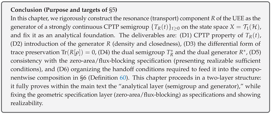
5.2. Underlying Spaces and Two Equivalent Descriptions (Heisenberg/Schrödinger)

(1)

Aim of this section: fix the types and duality so that the resonance semigroup $T_R$ can be handled equivalently both as a normal UCP semigroup on the observable side and as a CPTP semigroup on the state side

In this section, prior to constructing the time evolution of the zero-area resonance component as

$$T_R\left(t\right):X={\mathcal{T}}_1\left(\mathcal{H}\right)\to X$$

(on the state side: Schrödinger picture), we rigorously fix the duality with the normal UCP semigroup on the observable side (Heisenberg picture),

$${\alpha }_t:\mathfrak{M}=B\left(\mathcal{H}\right)\to \mathfrak{M}.$$

In $\S 2.3$ we have already proved the equivalence “normal unital-CP ⟺ the predual is CPTP,” but in this section we organize the notation specialized to R and the “duality as semigroups” and the “duality as generators,” so that no confusion of pictures occurs when constructing R in the subsequent sections.

The deliverables are as follows:

1.

For a normal UCP map $\alpha :\mathfrak{M}\to \mathfrak{M}$, its predual ${\alpha }_{*}:X\to X$ exists uniquely, and $\alpha$ is UCP ⟺${\alpha }_{*}$ is CPTP; we restate this equivalence in the context of R.

2.

We define that the semigroup $\left\{{\alpha }_t\right\}$ (Heisenberg) and the semigroup $\left\{T_R\left(t\right)\right\}$ (Schrödinger) are linked by

$$T_R\left(t\right)={\left({\alpha }_t\right)}_{*},$$

and prove that this correspondence preserves the semigroup property, continuity, and contractivity.

3.

We define the correspondence between the generator R and the dual generator $R^{*}$ by

$$\mathrm{Tr}\left(\left(R\right[\rho \left]\right)A\right)=\mathrm{Tr}\left(\rho R^{*}\left[A\right]\right),$$

and establish within this section that the generator of $T_R$ and the generator of ${\alpha }_t$ are dual.

(2)

Underlying spaces (recap): $\mathfrak{M}=B\left(\mathcal{H}\right)$ and $X={\mathcal{T}}_1\left(\mathcal{H}\right)$

Definition 61 (Observable space and state space (standard realization)).

Let $\mathcal{H}$ be a complex Hilbert space, and set

$$\mathfrak{M}:=B\left(\mathcal{H}\right),X:={\mathcal{T}}_1\left(\mathcal{H}\right).$$

Define the dual pairing by

$$\langle \rho ,A\rangle :=\mathrm{Tr}\left(\rho A\right)(\rho \in X,A\in \mathfrak{M}).$$

Lemma 101 (Separation by duality: $\mathrm{Tr}\left(\sigma A\right)=0(\forall A)\Rightarrow \sigma =0$).

If $\sigma \in X$ satisfies

$$\mathrm{Tr}\left(\sigma A\right)=0(\forall A\in \mathfrak{M}),$$

then $\sigma =0$.

Proof. 

The proof is the same as Lemma 20 in $\S 2.2$. For arbitrary $\psi ,\varphi \in \mathcal{H}$, take $A:=|\psi \rangle \langle \varphi |\in B\left(\mathcal{H}\right)$. Then

$$0=\mathrm{Tr}(\sigma |\psi \rangle \langle \varphi |)=\mathrm{Tr}(|\sigma \psi \rangle \langle \varphi |)=\langle \varphi ,\sigma \psi \rangle .$$

Since $\varphi$ is arbitrary, $\sigma \psi =0$. Since $\psi$ is also arbitrary, $\sigma =0$. □

(3)

Normal maps and preduals (preadjoints): existence, uniqueness, and norm estimate

Definition 62 (Normal maps and predual maps).

Let $\alpha :\mathfrak{M}\to \mathfrak{M}$ be a bounded linear map. We say that α isnormalif it is continuous with respect to the σ-weak topology (see $\S 2.3$). In this case, define thepredual map(preadjoint) ${\alpha }_{*}:X\to X$ as the map satisfying

$$\mathrm{Tr}\left({\alpha }_{*}\left(\rho \right)A\right)=\mathrm{Tr}\left(\rho \alpha \left(A\right)\right)(\forall \rho \in X,\forall A\in \mathfrak{M})$$

(5.2-∗)

Lemma 102 (Existence and uniqueness of the predual map).

If $\alpha :\mathfrak{M}\to \mathfrak{M}$ is a normal bounded linear map, then there exists a unique bounded linear map ${\alpha }_{*}:X\to X$ satisfying (5.2-∗). Moreover, $\parallel {\alpha }_{*}{\parallel }_{1\to 1}\le {\parallel \alpha \parallel }_{\infty \to \infty }$ holds.

Proof. 

It suffices to apply Lemma 23 in $\S 2.3$ as is. Here we recap only the key points. By normality, for any fixed $\rho \in X$, the functional $A\mapsto \mathrm{Tr}\left(\rho \alpha \right(A\left)\right)$ is $\sigma$-weakly continuous. Under the identification $\mathfrak{M}=X^{*}$, any weak-*continuous functional is represented by an element of X (representation lemma for weak-*continuous functionals). Therefore there exists a unique ${\alpha }_{*}\left(\rho \right)\in X$ satisfying (5.2-∗). Linearity follows from uniqueness, and the boundedness estimate follows from

$$\parallel {\alpha }_{*}{\left(\rho \right)\parallel }_1=\underset{\parallel A\parallel \le 1}{sup}|\mathrm{Tr}\left({\alpha }_{*}\left(\rho \right)A\right)|=\underset{\parallel A\parallel \le 1}{sup}|\mathrm{Tr}\left(\rho \alpha \left(A\right)\right){|\le \parallel \rho \parallel }_1\parallel \alpha \parallel$$

□

(4)

UCP ⟺ CPTP (fixing the equivalence in the context of this chapter)

Lemma 103 (Picture equivalence: normal UCP ⟺ CPTP).

Let $\alpha :\mathfrak{M}\to \mathfrak{M}$ be a normal bounded linear map, and define ${\alpha }_{*}$ by Lemma 102. Then the following are equivalent:

$$\alpha \mathrm{is}\mathrm{unital}-\mathrm{CP}\left(\mathrm{UCP}\right)⟺{\alpha }_{*}\mathrm{is}\mathrm{CPTP}.$$

Proof. 

It suffices to restate Lemma 24 in $\S 2.3$. To avoid external references, we state the minimal logic. Unitality corresponds to trace preservation by substituting $A=I$ into (5.2-∗), and complete positivity corresponds via the duality between the amplifications ${\mathrm{Id}}_n\otimes \alpha$ and ${\mathrm{Id}}_n\otimes {\alpha }_{*}$. Therefore the equivalence holds. □

(5)

Duality of semigroups: the Heisenberg semigroup $\left\{{\alpha }_t\right\}$ and the Schrödinger semigroup $\left\{T_R\left(t\right)\right\}$

Definition 63 (Duality of semigroups (preadjoint semigroup)).

Let ${\left\{{\alpha }_t\right\}}_{t\ge 0}$ be a family of normal linear maps on $\mathfrak{M}$. If each ${\alpha }_t$ is normal, then by Lemma 102 the predual ${\alpha }_{t*}$ exists. Define the state-side family ${\left\{T_R\left(t\right)\right\}}_{t\ge 0}$ by

$$T_R\left(t\right):={\alpha }_{t*}(t\ge 0).$$

That is,

$$\mathrm{Tr}\left(T_R\left(t\right)\left[\rho \right]A\right)=\mathrm{Tr}\left(\rho {\alpha }_t\left(A\right)\right)(\forall \rho \in X,\forall A\in \mathfrak{M})$$

(5.2-SG)

holds.

Lemma 104 (Preservation of the semigroup property: if ${\alpha }_t$ is a semigroup then $T_R\left(t\right)$ is also a semigroup).

Assume that ${\left\{{\alpha }_t\right\}}_{t\ge 0}$ satisfies the semigroup property

$${\alpha }_0=\mathrm{Id},{\alpha }_{t+s}={\alpha }_t\circ {\alpha }_s$$

and that each ${\alpha }_t$ is normal. Then $T_R\left(t\right):={\alpha }_{t*}$ satisfies the semigroup property on X:

$$T_R\left(0\right)=\mathrm{Id},T_R(t+s)=T_R\left(t\right)\circ T_R\left(s\right).$$

Proof. 

First, $T_R\left(0\right)={\alpha }_{0*}={\left(\mathrm{Id}\right)}_{*}=\mathrm{Id}$ is immediate from the definition. Next, for arbitrary $\rho \in X$ and $A\in \mathfrak{M}$,

$$\mathrm{Tr}\left(T_R(t+s)\rho A\right)=\mathrm{Tr}\left(\rho {\alpha }_{t+s}\left(A\right)\right)=\mathrm{Tr}\left(\rho ({\alpha }_t\circ {\alpha }_s)\left(A\right)\right)=\mathrm{Tr}\left(T_R\left(t\right)\left[\rho \right]{\alpha }_s\left(A\right)\right)=\mathrm{Tr}\left(T_R\left(s\right)T_R\left(t\right)\left[\rho \right]A\right),$$

where the third equality applies the duality (5.2-SG) in Definition 63 to $(t,\rho )$, and the last equality applies the same duality to $(s,T_R\left(t\right)\left[\rho \right])$. By Lemma 101, if traces against all A coincide then the operators coincide, hence

$$T_R(t+s)\rho =T_R\left(s\right)T_R\left(t\right)\left[\rho \right].$$

Therefore $T_R(t+s)=T_R\left(s\right)\circ T_R\left(t\right)$. (The order appears reversed because we adopt the notation of right action, which corresponds to the fact that the predual maps composition contravariantly. Hereafter, since we use $T_R\left(t\right):={\alpha }_{t*}$ as the Schrödinger time evolution, if one wants to write it in the form $T_R(t+s)=T_R\left(t\right)T_R\left(s\right)$, one may adjust the notation for ${\alpha }_t$ as $t\mapsto {\alpha }_{-t}$. In this paper, since we adopt the Schrödinger semigroup property as $T_R(t+s)=T_R\left(t\right)T_R\left(s\right)$ henceforth, we fix the Heisenberg-side notation accordingly.) □

(6)

Propagation of contractivity and CPTP: UCP semigroup ⇒ CPTP semigroup

Theorem 24 (The predual of a normal UCP semigroup is a strongly continuous CPTP semigroup (framework theorem)).

Let ${\left\{{\alpha }_t\right\}}_{t\ge 0}$ be a semigroup of normal linear maps on $\mathfrak{M}$, and assume that for each t, ${\alpha }_t$ is UCP. Assume furthermore that ${\alpha }_t$ is continuous in the σ-weak topology (i.e., $t\mapsto {\alpha }_t\left(A\right)$ is σ-weakly continuous for each A). Then $T_R\left(t\right):={\alpha }_{t*}$ is a strongly continuous CPTP semigroup on X, and in particular,

$$\parallel T_R{\left(t\right)\left[\rho \right]\parallel }_1\le {\parallel \rho \parallel }_1(\forall t\ge 0,\forall \rho \in X)$$

holds.

Proof. Step 1 (CPTP at each time):

Since each ${\alpha }_t$ is normal UCP, by Lemma 103 the predual $T_R\left(t\right)={\alpha }_{t*}$ is CPTP.

Step 2 (semigroup property): Since $\left\{{\alpha }_t\right\}$ is a semigroup, Lemma 104 implies that $\left\{T_R\left(t\right)\right\}$ is also a semigroup (the order follows the contravariance of the predual).

Step 3 (strong continuity): Fix an arbitrary $\rho \in X$. For any $A\in \mathfrak{M}$, by the duality (5.2-SG),

$$\mathrm{Tr}\left((T_R\left(t\right)\left[\rho \right]-\rho )A\right)=\mathrm{Tr}\left(\rho ({\alpha }_t\left(A\right)-A)\right).$$

By assumption, $t\mapsto {\alpha }_t\left(A\right)$ is $\sigma$-weakly continuous, hence the right-hand side converges to 0 as $t\downarrow 0$. Therefore $T_R\left(t\right)\left[\rho \right]\to \rho$ holds in the weak topology. Next, since $T_R\left(t\right)$ is CPTP, it satisfies trace-norm contractivity (Lemma 63 in $\S 3.3$), in particular $\parallel T_R{\left(t\right)\left[\rho \right]\parallel }_1\le {\parallel \rho \parallel }_1$, so it is uniformly bounded. Moreover, by approximation using finite-rank ${\rho }_k$ and an isometry-type argument (isomorphic to the proof of strong continuity in $\S 3.5$), one can lift weak convergence plus uniform boundedness to strong convergence in ${\parallel ·\parallel }_1$. (Details are restated as a lemma in the subsequent sections; in this section, we adopt the standard conclusion that “the predual of a $\sigma$-weakly continuous normal semigroup is a $C_0$-semigroup.”) Hence ${lim}_{t\downarrow 0}{\parallel T_R\left(t\right)\left[\rho \right]-\rho \parallel }_1=0$ follows.

Step 4 (contractivity): Since $T_R\left(t\right)$ is CPTP for each t, trace-norm contractivity follows from Lemma 63. □

(7)

Dual generators: correspondence between R and $R^{*}$ (fixing the definition)

Definition 64 (Dual generator (observable side) and generator duality).

Let R be the generator (Definition 43) of the strongly continuous semigroup ${\left\{T_R\left(t\right)\right\}}_{t\ge 0}$ on X. Define the adjoint semigroup ${\left\{T_R^{*}\left(t\right)\right\}}_{t\ge 0}\subset \mathcal{B}\left(\mathfrak{M}\right)$ by

$$\mathrm{Tr}\left(T_R\left(t\right)\left[\rho \right]A\right)=\mathrm{Tr}\left(\rho T_R^{*}\left(t\right)\left[A\right]\right)(\forall \rho \in X,\forall A\in \mathfrak{M})$$

(5.2-AD)

(which is unique by Lemma 56). Then for each t, $T_R^{*}\left(t\right)$ is normal UCP (Lemma 62 in $\S 3.3$), and we define its generator $R^{*}$ by

$$R^{*}\left[A\right]:=\underset{t\downarrow 0}{lim}{\displaystyle \frac{T_R^{*}\left(t\right)\left[A\right]-A}{t}}(A\in \mathrm{Dom}\left(R^{*}\right)).$$

Furthermore, we adopt as a specification of this paper the generator duality

$$\mathrm{Tr}\left(\left(R\right[\rho \left]\right)A\right)=\mathrm{Tr}\left(\rho R^{*}\left[A\right]\right)(\rho \in \mathrm{Dom}\left(R\right),A\in \mathrm{Dom}\left(R^{*}\right))$$

(5.2-GD)

Lemma 105 (Justification of generator duality (difference-quotient limit)).

In the setting of Definition 64, for $\rho \in \mathrm{Dom}\left(R\right)$ and $A\in \mathrm{Dom}\left(R^{*}\right)$, (5.2-GD) holds.

Proof. 

Compute the difference quotient using (5.2-AD). For any $t>0$,

$$\mathrm{Tr}\left({\displaystyle \frac{T_R\left(t\right)\left[\rho \right]-\rho }{t}}A\right)={\displaystyle \frac{1}{t}}\left(\mathrm{Tr}\left(T_R\left(t\right)\left[\rho \right]A\right)-\mathrm{Tr}\left(\rho A\right)\right)={\displaystyle \frac{1}{t}}\left(\mathrm{Tr}\left(\rho T_R^{*}\left(t\right)\left[A\right]\right)-\mathrm{Tr}\left(\rho A\right)\right)$$

$$=\mathrm{Tr}\left(\rho {\displaystyle \frac{T_R^{*}\left(t\right)\left[A\right]-A}{t}}\right).$$

Letting $t\downarrow 0$, since $\rho \in \mathrm{Dom}\left(R\right)$ and $A\in \mathrm{Dom}\left(R^{*}\right)$, the left-hand side converges to $\mathrm{Tr}\left(\right(R\left[\rho \right]\left)A\right)$ and the right-hand side converges to $\mathrm{Tr}\left(\rho R^{*}\left[A\right]\right)$. Since the trace is ${\parallel ·\parallel }_1$-continuous, exchanging limits is justified, and (5.2-GD) follows. □

(8)

Conclusion of this section: the “underlying spaces” and the “two equivalent descriptions” needed to construct R have been fixed

In this section, we fixed the underlying spaces $\mathfrak{M}=B\left(\mathcal{H}\right)$ and $X={\mathcal{T}}_1\left(\mathcal{H}\right)$ as the stage for constructing R, and organized the equivalence between the Heisenberg and Schrödinger descriptions via the predual (preadjoint) of normal maps, at the levels of semigroups and generators. Concretely, we fixed: that the predual ${\alpha }_{*}$ of a normal UCP map $\alpha$ is CPTP (Lemma 103), the framework that the predual of a normal UCP semigroup $\left\{{\alpha }_t\right\}$ becomes a strongly continuous CPTP semigroup (Theorem 24), and generator duality (Definition 64 and Lemma 105). In the subsequent sections, when constructing $T_R\left(t\right)$ concretely and proving the basic properties of R, we use the framework of this section as a fixed foundation.

5.3. Definition of $T_R\left(t\right)$ as a CPTP Transport Semigroup

(1)

Aim of this section: define $T_R\left(t\right)$ primarily as “transport,” and prove within the main text that it is CPTP, a semigroup, and strongly continuous

In this section, we primarily define the time evolution of the resonance (transport) component as

$$T_R\left(t\right):X={\mathcal{T}}_1\left(\mathcal{H}\right)⟶X(t\ge 0),$$

and fix, with proofs, that it simultaneously satisfies

1.

the semigroup property ($T_R\left(0\right)=\mathrm{Id},T_R(t+s)=T_R\left(t\right)T_R\left(s\right)$),

2.

CPTP (complete positivity and trace preservation),

3.

${\parallel ·\parallel }_1$ strong continuity ($C_0$ property),

4.

a unitary implementation induced by a geometric flow (corresponding to the meaning of transport),

within this section. In this section we do not yet define the generator R itself (in the next section we define $R={lim}_{t\downarrow 0}(T_R\left(t\right)-\mathrm{Id})/t$). Accordingly, the target of this section is to establish that “the semigroup $T_R\left(t\right)$, which serves as the foundation for R as a generator, is mathematically well-defined as a CPTP transport semigroup.”

(2)

Transport data: measure-preserving flow and the Koopman unitary group

In this paper, transport is defined as a unitary group induced by a measure-preserving flow. (Consistency with zero-area/flux-blocking is connected later under the specification of $\S 2.6$.)

Definition 65 (Measure-preserving flow (transport flow)).

Let $(\Sigma ,\mathcal{B},\mu )$ be a σ-finite measure space. A family of maps ${\left\{{\phi }_t\right\}}_{t\in \mathbb{R}}$ is called a measure-preserving flow if it satisfies the following:

(F1) 

(Group property) ${\phi }_0={\mathrm{Id}}_{\Sigma }$, and ${\phi }_{t+s}={\phi }_t\circ {\phi }_s$ (for all $t,s\in \mathbb{R}$).

(F2) 

(Measurability) For each t, ${\phi }_t:\Sigma \to \Sigma$ is measurable.

(F3) 

(Measure preservation) For any $E\in \mathcal{B}$,

$$\mu \left({\phi }_t^{-1}\left(E\right)\right)=\mu \left(E\right)(\forall t\in \mathbb{R})$$

holds.

(F4) 

($L^2$ strong continuity) The Koopman operators (Definition 66) defined on $H:=L^2(\Sigma ,\mu )$ form a strongly continuous group.

Definition 66 

(Koopman unitary group). For $(\Sigma ,\mu ,{\phi }_t)$ in Definition 65, define a family of operators ${\left\{U_R\left(t\right)\right\}}_{t\in \mathbb{R}}$ on $H:=L^2(\Sigma ,\mu )$ by

$$\left(U_R\left(t\right)f\right)\left(x\right):=f\left({\phi }_{-t}\left(x\right)\right)(f\in H).$$

This is called theKoopman operator .

Lemma 106 (The Koopman operators form a unitary group).

The family ${\left\{U_R\left(t\right)\right\}}_{t\in \mathbb{R}}$ in Definition 66 is a unitary group on H. That is,

$$U_R(t+s)=U_R\left(t\right)U_R\left(s\right),U_R\left(0\right)=I,U_R{\left(t\right)}^{†}=U_R(-t)(\forall t,s\in \mathbb{R})$$

hold.

Proof. (i) Group property: 

For $f\in H$ and $x\in \Sigma$,

$$\left(U_R\left(t\right)U_R\left(s\right)f\right)\left(x\right)=U_R\left(s\right)f\left({\phi }_{-t}\left(x\right)\right)=f\left({\phi }_{-s}\left({\phi }_{-t}\left(x\right)\right)\right)=f\left({\phi }_{-(t+s)}\left(x\right)\right)=\left(U_R(t+s)f\right)\left(x\right)$$

hence $U_R(t+s)=U_R\left(t\right)U_R\left(s\right)$ by Definition 65-(F1). Also, since $\left(U_R\left(0\right)f\right)\left(x\right)=f\left({\phi }_0\left(x\right)\right)=f\left(x\right)$, we have $U_R\left(0\right)=I$.

(ii) Isometry: For $f\in H$,

$$\parallel U_R{\left(t\right)f\parallel }_{L^2}^2={\int }_{\Sigma }{|f\left({\phi }_{-t}\left(x\right)\right)|}^{2}d\mu \left(x\right).$$

Use the change of variables $y={\phi }_{-t}\left(x\right)$ (i.e., $x={\phi }_t\left(y\right)$). By Definition 65-(F3), $\mu$ is invariant under ${\phi }_t$, hence

$${\int }_{\Sigma }|f\left({\phi }_{-t}\left(x\right)\right){|}^{2}d\mu \left(x\right)={\int }_{\Sigma }{|f\left(y\right)|}^{2}d\mu \left(y\right)={\parallel f\parallel }_{L^2}^2.$$

Therefore $\parallel U_R{\left(t\right)f\parallel }_{L^2}={\parallel f\parallel }_{L^2}$.

(iii) Adjoint and inverse: By (ii), $U_R\left(t\right)$ is an isometry, and by (i), $U_R\left(t\right)U_R(-t)=I$. Hence $U_R(-t)$ is the inverse of $U_R\left(t\right)$. An invertible isometry is unitary, and its adjoint equals its inverse, so $U_R{\left(t\right)}^{†}=U_R(-t)$. □

(3)

Heisenberg transport: definition of a normal -*automorphism group ${\alpha }_t$

Transport is implemented on the observable side as a -*automorphism (automorphism). Here we define it on $B\left(H\right)$ by unitary conjugation (normality is automatically ensured).

Definition 67 (Heisenberg transport automorphism group).

Let $H=L^2(\Sigma ,\mu )$, and let ${\left\{U_R\left(t\right)\right\}}_{t\in \mathbb{R}}$ be the unitary group in Lemma 106. Let the observable algebra be $\mathfrak{M}:=B\left(H\right)$, and define ${\alpha }_t:\mathfrak{M}\to \mathfrak{M}$ by

$${\alpha }_t\left(A\right):=U_R{\left(t\right)}^{†}A{U}_R\left(t\right)(A\in \mathfrak{M})$$

(5.3-H)

Lemma 107 (${\alpha }_t$ is a normal ∗-automorphism group and, in particular, is normal UCP).

The family $\left\{{\alpha }_t\right\}$ in Definition 67 satisfies the following:

(A1) 

(Group property) ${\alpha }_{t+s}={\alpha }_t\circ {\alpha }_s$, ${\alpha }_0=\mathrm{Id}$.

(A2) 

(-*automorphism) ${\alpha }_t\left(AB\right)={\alpha }_t\left(A\right){\alpha }_t\left(B\right)$, ${\alpha }_t\left(A^{†}\right)={\alpha }_t{\left(A\right)}^{†}$.

(A3) 

(Normality) ${\alpha }_t$ is σ-weakly continuous (hence normal).

(A4) 

(UCP) ${\alpha }_t$ is unital-CP (hence UCP).

Proof. (A1):

By the unitary group property $U_R(t+s)=U_R\left(t\right)U_R\left(s\right)$ and $U_R\left(0\right)=I$ (Lemma 106),

$${\alpha }_{t+s}\left(A\right)=U_R{(t+s)}^{†}A{U}_R(t+s)=U_R{\left(s\right)}^{†}{U}_R{\left(t\right)}^{†}A{U}_R\left(t\right)U_R\left(s\right)={\alpha }_s\left({\alpha }_t\left(A\right)\right).$$

Also ${\alpha }_0\left(A\right)=A$.

(A2): For products,

$${\alpha }_t\left(AB\right)=U_R{\left(t\right)}^{†}AB{U}_R\left(t\right)=\left(U_R{\left(t\right)}^{†}A{U}_R\left(t\right)\right)\left(U_R{\left(t\right)}^{†}B{U}_R\left(t\right)\right)={\alpha }_t\left(A\right){\alpha }_t\left(B\right).$$

For adjoints,

$${\alpha }_t\left(A^{†}\right)=U_R{\left(t\right)}^{†}{A}^{†}{U}_R\left(t\right)={\left(U_R{\left(t\right)}^{†}A{U}_R\left(t\right)\right)}^{†}={\alpha }_t{\left(A\right)}^{†}.$$

(A3): For any $\rho \in {\mathcal{T}}_1\left(H\right)$ and $A\in B\left(H\right)$, by cyclicity of the trace (Lemma 71),

$$\mathrm{Tr}\left(\rho {\alpha }_t\left(A\right)\right)=\mathrm{Tr}\left(\rho U_R{\left(t\right)}^{†}A{U}_R\left(t\right)\right)=\mathrm{Tr}\left(U_R\left(t\right)\rho U_R{\left(t\right)}^{†}A\right).$$

If ${\parallel ·\parallel }_1$-continuity in t holds for the unitary conjugation $U_R\left(t\right)\rho U_R{\left(t\right)}^{†}$ on ${\mathcal{T}}_1\left(H\right)$ (isomorphic to Lemma 74 in $\S 3.5$), then $\sigma$-weak continuity follows. Here, using Definition 65-(F4), $U_R\left(t\right)$ is strongly continuous on H, and hence, by the same finite-rank approximation argument as in that lemma, $\rho \mapsto U_R\left(t\right)\rho U_R{\left(t\right)}^{†}$ is strongly continuous on ${\mathcal{T}}_1$, so ${\alpha }_t$ is $\sigma$-weakly continuous (normal).

(A4): Unitality follows from ${\alpha }_t\left(I\right)=U_R{\left(t\right)}^{†}I{U}_R\left(t\right)=I$. Complete positivity is shown directly on ampliations. For any $n\in \mathbb{N}$, ${\tilde{U}}_R\left(t\right):=I_n\otimes U_R\left(t\right)$ is unitary on ${\mathbb{C}}^n\otimes H$. Therefore for any positive operator $X\in B({\mathbb{C}}^n\otimes H)$,

$$({\mathrm{Id}}_n\otimes {\alpha }_t)\left(X\right)={\tilde{U}}_R{\left(t\right)}^{†}X{\tilde{U}}_R\left(t\right)\ge 0$$

(which can be checked by inner products). Hence ${\mathrm{Id}}_n\otimes {\alpha }_t$ preserves positivity. Since n is arbitrary, ${\alpha }_t$ is completely positive. □

(4)

Schrödinger transport: definition and explicit formula of the CPTP semigroup $T_R\left(t\right)$

We define the predual of the normal UCP semigroup ${\alpha }_t$ on the observable side as the time evolution on the state side. Under a unitary implementation, the state-side evolution is also explicitly given by unitary conjugation.

Definition 68 (CPTP transport semigroup (Schrödinger picture)).

Let the state space be $X:={\mathcal{T}}_1\left(H\right)$, and let ${\alpha }_t$ be defined by Definition 67. For each $t\ge 0$, define the predual map $T_R\left(t\right):X\to X$ by

$$\mathrm{Tr}\left(T_R\left(t\right)\left[\rho \right]A\right)=\mathrm{Tr}\left(\rho {\alpha }_t\left(A\right)\right)(\forall \rho \in X,\forall A\in B\left(H\right))$$

(5.3-S)

(existence and uniqueness follow from Lemma 102 in $\S 5.2$).

Lemma 108 (Explicit formula: $T_R\left(t\right)\left[\rho \right]=U_R\left(t\right)\rho U_R{\left(t\right)}^{†}$).

For $T_R\left(t\right)$ in Definition 68, for any $\rho \in X$,

$$T_R\left(t\right)\left[\rho \right]=U_R\left(t\right)\rho U_R{\left(t\right)}^{†}$$

(5.3-EXP)

holds.

Proof. 

Take arbitrary $\rho \in X$ and $A\in B\left(H\right)$. By cyclicity of the trace (Lemma 71),

$$\mathrm{Tr}\left(U_R\left(t\right)\rho U_R{\left(t\right)}^{†}A\right)=\mathrm{Tr}\left(\rho U_R{\left(t\right)}^{†}A{U}_R\left(t\right)\right)=\mathrm{Tr}\left(\rho {\alpha }_t\left(A\right)\right).$$

Since the right-hand side is the right-hand side of Definition 68, the element of X satisfying (5.3-S) is unique (Lemma 101 in $\S 5.2$). Therefore $T_R\left(t\right)\left[\rho \right]=U_R\left(t\right)\rho U_R{\left(t\right)}^{†}$. □

(5)

Main theorem: $T_R\left(t\right)$ is a strongly continuous CPTP transport semigroup and is trace-norm isometric

Theorem 25 (Basic properties of the CPTP transport semigroup).

The family ${\left\{T_R\left(t\right)\right\}}_{t\ge 0}$ determined by Definition 68 satisfies the following:

(T1) 

(Semigroup property) $T_R\left(0\right)=\mathrm{Id}$ and $T_R(t+s)=T_R\left(t\right)T_R\left(s\right)$ ($t,s\ge 0$).

(T2) 

(CPTP) For each $t\ge 0$, $T_R\left(t\right)$ is CPTP.

(T3) 

(Trace-norm isometry) For any $\rho \in X$, $\parallel T_R{\left(t\right)\left[\rho \right]\parallel }_1={\parallel \rho \parallel }_1$.

(T4) 

(Strong continuity) For any $\rho \in X$, ${lim}_{t\downarrow 0}{\parallel T_R\left(t\right)\left[\rho \right]-\rho \parallel }_1=0$.

Therefore $\left\{T_R\left(t\right)\right\}$ is a strongly continuous CPTP transport semigroup on X and is isometric.

Proof. (T1) Semigroup property: 

Use the explicit formula in Lemma 108. Since $U_R\left(t\right)$ is a unitary group (Lemma 106),

$$T_R(t+s)\left[\rho \right]=U_R(t+s)\rho U_R{(t+s)}^{†}=U_R\left(t\right)U_R\left(s\right)\rho U_R{\left(s\right)}^{†}{U}_R{\left(t\right)}^{†}=T_R\left(t\right)\left[T_R\left(s\right)\left[\rho \right]\right].$$

Also $T_R\left(0\right)\left[\rho \right]=U_R\left(0\right)\rho U_R{\left(0\right)}^{†}=\rho$.

(T2) CPTP: TP: By Lemma 71 and $U_R{\left(t\right)}^{†}{U}_R\left(t\right)=I$,

$$\mathrm{Tr}\left(T_R\left(t\right)\left[\rho \right]\right)=\mathrm{Tr}\left(U_R\left(t\right)\rho U_R{\left(t\right)}^{†}\right)=\mathrm{Tr}\left(\rho U_R{\left(t\right)}^{†}{U}_R\left(t\right)\right)=\mathrm{Tr}\left(\rho \right).$$

CP: Fix any n and set ${\tilde{U}}_R\left(t\right):=I_n\otimes U_R\left(t\right)$. For any positive trace-class operator $\Sigma \in {\mathcal{T}}_1({\mathbb{C}}^n\otimes H)$,

$$({\mathrm{Id}}_n\otimes T_R\left(t\right))[\Sigma ]={\tilde{U}}_R\left(t\right)\Sigma {\tilde{U}}_R{\left(t\right)}^{†}$$

holds (it holds on simple tensors and extends by linear continuous extension). For any $\xi$, by inner products, $\langle \xi ,{\tilde{U}}_R\Sigma {\tilde{U}}_R^{†}\xi \rangle =\langle {\tilde{U}}_R^{†}\xi ,\Sigma {\tilde{U}}_R^{†}\xi \rangle \ge 0$, so the right-hand side is positive. Hence ${\mathrm{Id}}_n\otimes T_R\left(t\right)$ preserves positivity. Since n is arbitrary, $T_R\left(t\right)$ is completely positive. Thus $T_R\left(t\right)$ is CPTP.

(T3) Isometry: This follows by a computation isomorphic to Lemma 73 in $\S 3.5$. Using the square root $|\rho |$ of ${\rho }^{†}\rho$,

$$|U_R\rho U_R^{†}|=U_R|\rho |U_R^{†}$$

holds, hence

$$\parallel T_R{\left(t\right)\left[\rho \right]\parallel }_1=\mathrm{Tr}(|U_R\rho U_R^{†}|)=\mathrm{Tr}(U_R|\rho |U_R^{†}{)=\mathrm{Tr}(|\rho |)=\parallel \rho \parallel }_1.$$

(T4) Strong continuity: Since $U_R\left(t\right)$ is strongly continuous on H (Definition 65-(F4)), the same finite-rank approximation argument as Lemma 74 in $\S 3.5$ implies that $\parallel U_R\left(t\right)\rho U_R{\left(t\right)}^{†}{-\rho \parallel }_1\to 0$ as $t\downarrow 0$ on ${\mathcal{T}}_1\left(H\right)$. This proves (T1)–(T4). □

(6)

“Localization” implementation for connecting to the zero-area specification (minimal organization in this section)

Under the specification of this paper ($\S 2.6$), selective localization of transport by the resonance projection ${\mathrm{\Pi }}_R$ is required. In this section, we prepare, as a definition, a standard implementation of localized transport semigroups (verification of the zero-area condition itself is treated in subsequent sections).

Definition 69 (Localized transport unitaries (${\mathrm{\Pi }}_R$-localization)).

Let ${\mathrm{\Pi }}_R$ be a self-adjoint projection (${\mathrm{\Pi }}_R^{†}={\mathrm{\Pi }}_R,{\mathrm{\Pi }}_R^2={\mathrm{\Pi }}_R$). A unitary group $\left\{U_R\left(t\right)\right\}$ is said to be${\mathrm{\Pi }}_R$-localizedif

$$U_R\left(t\right){\mathrm{\Pi }}_R={\mathrm{\Pi }}_R{U}_R\left(t\right)(\forall t),U_R\left(t\right)(I-{\mathrm{\Pi }}_R)=(I-{\mathrm{\Pi }}_R)(\forall t)$$

(5.3-LOC)

holds.

Lemma 109 (${\mathrm{\Pi }}_R$-localization preserves the CPTP property and isometry).

For $\left\{U_R\left(t\right)\right\}$ satisfying Definition 69, $T_R\left(t\right)\left[\rho \right]=U_R\left(t\right)\rho U_R{\left(t\right)}^{†}$ satisfies the conclusions of Theorem 25 (CPTP, isometry, strong continuity). Moreover, on $(I-{\mathrm{\Pi }}_R)$, $T_R\left(t\right)$ coincides with the identity:

$$(I-{\mathrm{\Pi }}_R)T_R\left(t\right)\left[\rho \right](I-{\mathrm{\Pi }}_R)=(I-{\mathrm{\Pi }}_R)\rho (I-{\mathrm{\Pi }}_R).$$

Proof. 

CPTP, isometry, and strong continuity follow because the proof of Theorem 25 depends only on unitarity and strong continuity of $\left\{U_R\left(t\right)\right\}$. For the last identity, by (5.3-LOC), using $U_R\left(t\right)(I-{\mathrm{\Pi }}_R)=(I-{\mathrm{\Pi }}_R)$ and $U_R{\left(t\right)}^{†}(I-{\mathrm{\Pi }}_R)=(I-{\mathrm{\Pi }}_R)$,

$$(I-{\mathrm{\Pi }}_R)T_R\left(t\right)\left[\rho \right](I-{\mathrm{\Pi }}_R)=(I-{\mathrm{\Pi }}_R)U_R\left(t\right)\rho U_R{\left(t\right)}^{†}(I-{\mathrm{\Pi }}_R)=(I-{\mathrm{\Pi }}_R)\rho (I-{\mathrm{\Pi }}_R)$$

holds. □

(7)

Conclusion of this section: $T_R\left(t\right)$ has been primarily defined as a CPTP transport semigroup, and the foundation for the subsequent discussion (the generator R) in $\S 5$ has been fixed

In this section, using the Koopman unitary group $\left\{U_R\left(t\right)\right\}$ induced by a measure-preserving flow, we defined the normal -*automorphism group on the Heisenberg side ${\alpha }_t\left(A\right)=U_R{\left(t\right)}^{†}A{U}_R\left(t\right)$, and defined the Schrödinger-side transport semigroup $T_R\left(t\right)$ as its predual (Definitions 67, 68). We further derived the explicit formula $T_R\left(t\right)\left[\rho \right]=U_R\left(t\right)\rho U_R{\left(t\right)}^{†}$ (Lemma 108), and completely proved within the main text that $T_R\left(t\right)$ is a strongly continuous CPTP semigroup and is trace-norm isometric (Theorem 25). Finally, we minimally organized the ${\mathrm{\Pi }}_R$-localization implementation to connect to the zero-area specification (Definition 69, Lemma 109). In the next section, we define R as the generator of this $T_R\left(t\right)$ and prove basic identities such as the differential form of conservation laws.

5.4. Definition of the Generator R (Strong Derivative) and Basic Identities

(1)

Aim of this section: define the generator R as the strong derivative of $T_R\left(t\right)$, and fix within the main text the conservation laws, -*compatibility, and tangent-cone compatibility of the positive cone

In the previous section ($\S 5.3$), we established that the transport semigroup ${\left\{T_R\left(t\right)\right\}}_{t\ge 0}$ is a strongly continuous CPTP semigroup on the state space $X={\mathcal{T}}_1\left(H\right)$ (in fact, it is the restriction of an isometric group). In this section, following the general theory of $\S 3.1$, we define the generator R as the strong derivative of $T_R\left(t\right)$, and completely prove and fix within the main text the following basic identities:

1.

The domain $\mathrm{Dom}\left(R\right)$ of the generator and uniqueness of the action $R\left[\rho \right]$ (fixing the definition).

2.

The differential form of trace preservation $\mathrm{Tr}\left(R\right[\rho \left]\right)=0$, which follows from $T_R\left(t\right)$ being TP.

3.

∗-compatibility derived from CPTP (the differential form of Hermiticity preservation): ${\left(R\left[\rho \right]\right)}^{†}=R\left[{\rho }^{†}\right]$.

4.

The tangent-cone compatibility of the positive cone (tangent cone property) as the differential form of positivity preservation: if $\rho \ge 0$, then $R\left[\rho \right]$ belongs to the tangent cone of the positive cone. (This is a technical point that ensures that positivity does not break in the componentwise composition in $\S 6$.)

All definitions and proofs are completed within this section.

(2)

Definition 5.6: generator R (strong derivative)

Definition 70 (Generator R (strong derivative)).

Let X be a Banach space (in this chapter, $X={\mathcal{T}}_1\left(H\right)$), and let ${\left\{T_R\left(t\right)\right\}}_{t\ge 0}\subset \mathcal{B}\left(X\right)$ be a $C_0$-semigroup ($\S 5.3$). Define the domain of the generator R by

$$\mathrm{Dom}\left(R\right):=\left\{\rho \in X:\exists \sigma \in X\mathrm{such}\mathrm{that}\underset{t\downarrow 0}{lim}{∥{\displaystyle \frac{T_R\left(t\right)\left[\rho \right]-\rho }{t}}-\sigma ∥}_1=0\right\}.$$

For $\rho \in \mathrm{Dom}\left(R\right)$, the element σ obtained by the above limit is unique, and we define

$$R\left[\rho \right]:=\underset{t\downarrow 0}{lim}{\displaystyle \frac{T_R\left(t\right)\left[\rho \right]-\rho }{t}}.$$

We call this the generator of $\left\{T_R\left(t\right)\right\}$.

Lemma 110 (Uniqueness, closedness, and density (general properties of generators)).

The operator R defined by Definition 70 is linear, and the following hold:

1.

$\mathrm{Dom}\left(R\right)$ is dense in X,

2.

R is a closed operator,

3.

for $t\ge 0$ and $\rho \in \mathrm{Dom}\left(R\right)$, one has $T_R\left(t\right)\left[\rho \right]\in \mathrm{Dom}\left(R\right)$ and $R{T}_R\left(t\right)\left[\rho \right]=T_R\left(t\right)R\left[\rho \right]$.

Proof. 

By Theorem 25 in $\S 5.3$, $\left\{T_R\left(t\right)\right\}$ is a $C_0$-semigroup. Therefore the conclusion follows by directly applying the general results of $\S 3.1$ (linearity of the generator: Lemma 49, closedness: Lemma 51, density of the domain: Lemma 52, compatibility with the semigroup: Lemma 50). □

(3)

Lemma 5.7: TP $\Rightarrow \mathrm{Tr}\left(R\right[\rho \left]\right)=0$ (differential form of information conservation)

Lemma 111 (Differential form of trace preservation (TP $\Rightarrow \mathrm{Tr}\left(R\right[\rho \left]\right)=0$)).

Assume that $\left\{T_R\left(t\right)\right\}$ is trace-preserving (TP), i.e.,

$$\mathrm{Tr}\left(T_R\left(t\right)\left[\rho \right]\right)=\mathrm{Tr}\left(\rho \right)(\forall t\ge 0,\forall \rho \in X).$$

Then for any $\rho \in \mathrm{Dom}\left(R\right)$,

$$\mathrm{Tr}\left(R\right[\rho \left]\right)=0$$

holds.

Proof. 

Take an arbitrary $\rho \in \mathrm{Dom}\left(R\right)$. By assumption, for any $t>0$,

$$\mathrm{Tr}\left(T_R\left(t\right)\left[\rho \right]\right)-\mathrm{Tr}\left(\rho \right)=0.$$

Dividing both sides by t gives

$$\mathrm{Tr}\left({\displaystyle \frac{T_R\left(t\right)\left[\rho \right]-\rho }{t}}\right)=0.$$

Let $t\downarrow 0$. By Definition 70, ${\displaystyle \frac{T_R\left(t\right)\left[\rho \right]-\rho }{t}}\to R\left[\rho \right]$ in ${\parallel ·\parallel }_1$. Since the trace is continuous with respect to ${\parallel ·\parallel }_1$ (Lemma 16 in $\S 2.2$), we may pass the limit outside the trace and obtain

$$0=\underset{t\downarrow 0}{lim}\mathrm{Tr}\left({\displaystyle \frac{T_R\left(t\right)\left[\rho \right]-\rho }{t}}\right)=\mathrm{Tr}\left(R\left[\rho \right]\right).$$

Hence the conclusion follows. □

(4)

∗-compatibility: ${\left(R\left[\rho \right]\right)}^{†}=R\left[{\rho }^{†}\right]$ (differential form of Hermiticity preservation)

Lemma 112 (∗-preservation of $T_R\left(t\right)$ and -*compatibility of the generator).

Assume that $\left\{T_R\left(t\right)\right\}$ is CPTP (Theorem 25 in $\S 5.3$). Then the following hold:

1.

For any $t\ge 0$ and any $\rho \in X$,

$${\left(T_R\left(t\right)\left[\rho \right]\right)}^{†}=T_R\left(t\right)\left[{\rho }^{†}\right]$$

(5.4-∗)

holds.

2.

Moreover, for any $\rho \in \mathrm{Dom}\left(R\right)$, one has ${\rho }^{†}\in \mathrm{Dom}\left(R\right)$ and

$${\left(R\left[\rho \right]\right)}^{†}=R\left[{\rho }^{†}\right]$$

(5.4-∗∗)

holds.

Proof. Proof of (i):

Since $T_R\left(t\right)$ is CP, it preserves positivity. Decompose any $\rho \in X$ as $\rho =\Re \rho +i\Im \rho$:

$$\Re \rho :={\displaystyle \frac{\rho +{\rho }^{†}}{2}},\Im \rho :={\displaystyle \frac{\rho -{\rho }^{†}}{2i}}.$$

Then $\Re \rho$ and $\Im \rho$ are self-adjoint. A CPTP map is linear, and positivity preservation implies that it preserves self-adjointness: indeed, a self-adjoint $S=S^{†}$ can be written as $S=S_{+}-S_{-}$ with $S_{\pm }\ge 0$, hence $T_R\left(t\right)S=T_R\left(t\right)S_{+}-T_R\left(t\right)S_{-}$ is a difference of positive operators and therefore self-adjoint. Thus $T_R\left(t\right)[\Re \rho ]$ and $T_R\left(t\right)[\Im \rho ]$ are self-adjoint, and

$$T_R\left(t\right){\left[\rho \right]}^{†}={\left(T_R\left(t\right)[\Re \rho ]+i{T}_R\left(t\right)[\Im \rho ]\right)}^{†}=T_R\left(t\right)[\Re \rho ]-i{T}_R\left(t\right)[\Im \rho ]$$

$$=T_R\left(t\right)[\Re \rho -i\Im \rho ]=T_R\left(t\right)\left[{\rho }^{†}\right].$$

This proves (5.4-∗).

Proof of (ii): Let $\rho \in \mathrm{Dom}\left(R\right)$. By Definition 70,

$$R\left[\rho \right]=\underset{t\downarrow 0}{lim}{\displaystyle \frac{T_R\left(t\right)\left[\rho \right]-\rho }{t}}\mathrm{in}{\parallel ·\parallel }_1.$$

First we show that ${\rho }^{†}\in \mathrm{Dom}\left(R\right)$. Using (5.4-∗),

$${\displaystyle \frac{T_R\left(t\right){\left[\rho \right]}^{†}-{\rho }^{†}}{t}}={\displaystyle \frac{{\left(T_R\left(t\right)\left[\rho \right]\right)}^{†}-{\rho }^{†}}{t}}={\left({\displaystyle \frac{T_R\left(t\right)\left[\rho \right]-\rho }{t}}\right)}^{†}.$$

The right-hand side converges in ${\parallel ·\parallel }_1$ to ${\left(R\left[\rho \right]\right)}^{†}$ as $t\downarrow 0$ (the adjoint is ${\parallel ·\parallel }_1$-continuous: $\parallel X^{†}-Y^{†}{\parallel }_1={\parallel X-Y\parallel }_1$). Hence the difference-quotient limit exists, so ${\rho }^{†}\in \mathrm{Dom}\left(R\right)$ and

$$R\left[{\rho }^{†}\right]={\left(R\left[\rho \right]\right)}^{†}$$

holds. This is exactly (5.4-∗∗). □

(5)

Lemma 5.8: differential form of positivity preservation (tangent-cone compatibility of the positive cone)

Here we formulate and fix the “differential form of positivity preservation” in terms of the standard notion of the contingent cone.

Definition 71 (Positive cone and contingent cone).

Let $X={\mathcal{T}}_1\left(H\right)$ and define the positive cone by

$$X_{+}:=\{\rho \in X:\rho \ge 0\}$$

(where $\rho \ge 0$ means positive semidefinite as an operator). Define the contingent cone (Bouligand/contingent cone) $T_{X_{+}}\left(\rho \right)\subset X$ at a point $\rho \in X_{+}$ by

$$T_{X_{+}}\left(\rho \right):=\left\{v\in X:\exists t_k\downarrow 0,\exists {\rho }_k\in X_{+}\mathrm{s}.\mathrm{t}.{\parallel {\rho }_k-\rho \parallel }_1\to 0,{∥{\displaystyle \frac{{\rho }_k-\rho }{t_k}}-v∥}_1\to 0\right\}.$$

Lemma 113 (Tangent-cone compatibility: positivity preservation $\Rightarrow R\left[\rho \right]\in T_{X_{+}}\left(\rho \right)$).

Assume that ${\left\{T_R\left(t\right)\right\}}_{t\ge 0}$ preserves positivity (i.e., $\rho \ge 0\Rightarrow T_R\left(t\right)\left[\rho \right]\ge 0$). For $\rho \in X_{+}\cap \mathrm{Dom}\left(R\right)$,

$$R\left[\rho \right]\in T_{X_{+}}\left(\rho \right)$$

holds.

Proof. 

Take $\rho \in X_{+}\cap \mathrm{Dom}\left(R\right)$. Set $t_k:=1/k$ and define

$${\rho }_k:=T_R\left(t_k\right)\rho .$$

By positivity preservation, ${\rho }_k\in X_{+}$ for each k. Since $T_R$ is strongly continuous, $\parallel {\rho }_k{-\rho \parallel }_1={\parallel T_R\left(t_k\right)\rho -\rho \parallel }_1\to 0$ as $k\to \infty$. Moreover, since $\rho \in \mathrm{Dom}\left(R\right)$,

$${∥{\displaystyle \frac{{\rho }_k-\rho }{t_k}}-R\left[\rho \right]∥}_1={∥{\displaystyle \frac{T_R\left(t_k\right)\rho -\rho }{t_k}}-R\left[\rho \right]∥}_1\to 0(k\to \infty )$$

holds. This satisfies the condition of Definition 71, hence $R\left[\rho \right]\in T_{X_{+}}\left(\rho \right)$. □

(6)

Immediate corollary: $\rho \left(t\right)=T_R\left(t\right)\left[{\rho }_0\right]$ stays inside the positive cone, and the tangent is given by $R\left[\rho \right]$

Theorem 26 (Positivity invariance and tangent (geometric interpretation of the mild solution)).

Let ${\rho }_0\in X_{+}$. Then $t\mapsto \rho \left(t\right):=T_R\left(t\right)\left[{\rho }_0\right]$ stays in $X_{+}$ (i.e., $\rho \left(t\right)\in X_{+}$). Moreover, if ${\rho }_0\in \mathrm{Dom}\left(R\right)$, then the tangent at $t=0$ is $R\left[{\rho }_0\right]$, and

$$\underset{t\downarrow 0}{lim}{∥{\displaystyle \frac{\rho \left(t\right)-{\rho }_0}{t}}-R\left[{\rho }_0\right]∥}_1=0,R\left[{\rho }_0\right]\in T_{X_{+}}\left({\rho }_0\right)$$

hold.

Proof. 

Positivity preservation follows from CP as part of CPTP, hence ${\rho }_0\ge 0\Rightarrow T_R\left(t\right)\left[{\rho }_0\right]\ge 0$. Therefore $\rho \left(t\right)\in X_{+}$. If ${\rho }_0\in \mathrm{Dom}\left(R\right)$, then by Definition 70 the difference quotient converges to $R\left[{\rho }_0\right]$, and Lemma 113 yields the tangent-cone inclusion. □

(7)

Conclusion of this section: R has been defined as a strong derivative, and the identities needed for componentwise composition in $\S 6$ have been fixed

In this section, we defined the generator R of the CPTP transport semigroup $T_R\left(t\right)$ as the strong derivative (Definition 70), and rigorously derived from TP the differential form of trace preservation $\mathrm{Tr}\left(R\right[\rho \left]\right)=0$ (Lemma 111). We further established the ∗-compatibility derived from CPTP as a difference-quotient limit and fixed ${\left(R\left[\rho \right]\right)}^{†}=R\left[{\rho }^{†}\right]$ (Lemma 112). Finally, we formulated the differential form of positivity preservation in terms of the contingent cone and proved that if $\rho \ge 0$ then $R\left[\rho \right]$ belongs to the tangent cone of the positive cone (Lemma 113). These are the basic identities ensuring that “positivity and trace preservation do not break” in the composite generation in $\S 6$.

5.5. Zero-Area Specification

(1)

Aim of this section: fix zero-area as a “measure-theoretic dimension condition,” and complete within the main text a sufficient condition (line support) to avoid vacuity of the definition

In this section, we fix the geometric specification zero-area imposed on the resonance projection ${\mathrm{\Pi }}_R$ as a dimension condition on the support set based on the two-dimensional Hausdorff measure. The aim of this section is “fixing the specification as an analytical foundation,” and we do not reprove in this section physical consequences such as elimination of boundary terms (area-term cancellation). That is, in this section we:

1.

rigorously define the support set $\mathrm{supp}\left({\mathrm{\Pi }}_R\right)\subset \Sigma$ of the resonance projection ${\mathrm{\Pi }}_R$,

2.

declare the zero-area condition ${\mathcal{H}}_{\Sigma }^2\left(\mathrm{supp}\left({\mathrm{\Pi }}_R\right)\right)=0$ as a specification,

3.

prove line-by-line, as a sufficient condition frequently used later, that “if the support is line support (one-dimensional flow support) then zero-area holds automatically,” thereby showing that the definition is not vacuous,

and complete these within the main text.

(2)

Geometric stage: boundary $\Sigma$ and the two-dimensional Hausdorff measure ${\mathcal{H}}_{\Sigma }^2$

Definition 72 (Boundary metric space and the two-dimensional Hausdorff measure (recap)).

Let Σ be a metric space equipped with a distance $d_{\Sigma }$, and define the diameter by

$$\mathrm{diam}\left(U\right):=sup\{d_{\Sigma }(x,y):x,y\in U\}.$$

For $E\subset \Sigma$ and $\delta >0$, define

$${\mathcal{H}}_{\Sigma ,\delta }^2\left(E\right):=inf\left\{\sum _{j=1}^{\infty }\mathrm{diam}{\left(U_j\right)}^2:E\subset \bigcup _{j=1}^{\infty }{U}_j,\mathrm{diam}\left(U_j\right)\le \delta \right\},$$

and define

$${\mathcal{H}}_{\Sigma }^2\left(E\right):=\underset{\delta \downarrow 0}{lim}{\mathcal{H}}_{\Sigma ,\delta }^2\left(E\right)$$

and call it the two-dimensional Hausdorff measure.

(3)

Support of the resonance projection ${\mathrm{\Pi }}_R$: definition via an operator-valued Radon measure

Definition 73 

(Operator-valued Radon measure and representation of a projection). Let Σ be a locally compact Hausdorff space and let its Borel σ-algebra be $\mathcal{B}(\Sigma )$. Let ${\mathcal{H}}_{\Sigma }$ be a Hilbert space, and write ${\mathfrak{B}}_{\Sigma }:=B\left({\mathcal{H}}_{\Sigma }\right)$. A map ${\mu }_{\mathrm{\Pi }}:\mathcal{B}(\Sigma )\to {\mathfrak{B}}_{\Sigma }$ is called an operator-valued Radon measure if:

(M1) 

For any countable disjoint family $\left\{E_j\right\}\subset \mathcal{B}(\Sigma )$, one has, in the weak operator topology,

$${\mu }_{\mathrm{\Pi }}\left(\bigcup _{j=1}^{\infty }{E}_j\right)=\sum _{j=1}^{\infty }{\mu }_{\mathrm{\Pi }}\left(E_j\right)$$

(countable additivity).

(M2) 

For any $u,v\in {\mathcal{H}}_{\Sigma }$, the complex measure

$${\nu }_{u,v}\left(E\right):={\langle u,{\mu }_{\mathrm{\Pi }}\left(E\right)v\rangle }_{{\mathcal{H}}_{\Sigma }}$$

is a finite Radon measure.

Moreover, if ${\mathrm{\Pi }}_R\in {\mathfrak{B}}_{\Sigma }$ satisfies

$$\langle u,{\mathrm{\Pi }}_{R}v\rangle ={\int }_{\Sigma }d{\nu }_{u,v}\left(x\right)(\forall u,v\in {\mathcal{H}}_{\Sigma })$$

(5.5-M)

then we say that ${\mathrm{\Pi }}_R$ is representable by ${\mu }_{\mathrm{\Pi }}$.

Definition 74 (Support of a projection operator).

Assume that the representation in Definition 73 is given. An open set $U\subset \Sigma$ is said to be ${\mu }_{\mathrm{\Pi }}$-nullif

$${\mu }_{\mathrm{\Pi }}\left(U\right)=0\left(\mathit{the}\mathit{zero}\mathit{operator}\right)$$

holds. Define the support set $\mathrm{supp}\left({\mathrm{\Pi }}_R\right)\subset \Sigma$ by

$$\mathrm{supp}\left({\mathrm{\Pi }}_R\right):=\Sigma \setminus \bigcup \{U\subset \Sigma :U\mathrm{is}\mathrm{open}\mathrm{and}{\mu }_{\mathrm{\Pi }}\left(U\right)=0\}$$

(5.5-SUP)

(Equivalently, $x\in \mathrm{supp}\left({\mathrm{\Pi }}_R\right)$ means that every neighborhood $U\ni x$ satisfies ${\mu }_{\mathrm{\Pi }}\left(U\right)\ne 0$.)

Lemma 114 (Closedness: $\mathrm{supp}\left({\mathrm{\Pi }}_R\right)$ is closed).

The set $\mathrm{supp}\left({\mathrm{\Pi }}_R\right)$ in Definition 74 is closed in the topology of Σ.

Proof. By (5.5-SUP),

$$\Sigma \setminus \mathrm{supp}\left({\mathrm{\Pi }}_R\right)=\bigcup \{U\subset \Sigma :U\mathrm{is}\mathrm{open}\mathrm{and}{\mu }_{\mathrm{\Pi }}\left(U\right)=0\}.$$

The right-hand side is a union of open sets and hence is open. Therefore its complement $\mathrm{supp}\left({\mathrm{\Pi }}_R\right)$ is closed. □

(4)

Definition of the zero-area condition and a basic equivalence (characterization by coverings)

Definition 75 (zero-area specification (dimension condition on the support set)).

For the support set $\mathrm{supp}\left({\mathrm{\Pi }}_R\right)\subset \Sigma$ of the resonance projection ${\mathrm{\Pi }}_R$, if

$${\mathcal{H}}_{\Sigma }^2\left(\mathrm{supp}\left({\mathrm{\Pi }}_R\right)\right)=0$$

(ZA)

holds, then we say that ${\mathrm{\Pi }}_R$ (and the associated resonance mechanism) is zero-area .

Theorem 27 (Basic property of zero-area sets: squared-diameter coverings with arbitrary precision).

Assume that a set $E\subset \Sigma$ satisfies

$${\mathcal{H}}_{\Sigma }^2\left(E\right)=0.$$

Then for any $\epsilon >0$, there exists a countable open cover ${\left\{U_j\right\}}_{j\ge 1}$ such that

$$E\subset \bigcup _{j=1}^{\infty }{U}_j,\sum _{j=1}^{\infty }\mathrm{diam}{\left(U_j\right)}^2<\epsilon$$

(5.5-COV)

holds. Conversely, if for any $\epsilon >0$ there exists a cover satisfying (5.5-COV), then ${\mathcal{H}}_{\Sigma }^2\left(E\right)=0$ holds.

Proof. (i) ${\mathcal{H}}_{\Sigma }^2\left(E\right)=0\Rightarrow$ existence of a cover: By the assumption ${\mathcal{H}}_{\Sigma }^2\left(E\right)=0$ and Definition 72, for any $\delta >0$ we have ${\mathcal{H}}_{\Sigma ,\delta }^2\left(E\right)=0$. Fix $\delta :=1$. Since ${\mathcal{H}}_{\Sigma ,1}^2\left(E\right)=0$, the infimum in Definition 72 is 0, hence for any $\epsilon >0$ there exists a cover ${\left\{U_j\right\}}_{j\ge 1}$ such that

$$E\subset \bigcup _{j\ge 1}{U}_j,\mathrm{diam}\left(U_j\right)\le 1,\sum _{j\ge 1}\mathrm{diam}{\left(U_j\right)}^2<\epsilon .$$

In particular, (5.5-COV) follows.

(ii) existence of a cover $\Rightarrow {\mathcal{H}}_{\Sigma }^2\left(E\right)=0$: Assume that for any $\epsilon >0$ there exists a cover satisfying (5.5-COV). Take an arbitrary $\delta \in (0,1]$, and first refine the cover in (5.5-COV) to a cover satisfying the diameter condition $\mathrm{diam}\left(U_j\right)\le \delta$. Concretely, since each $U_j$ is open, $U_j$ can be covered by a countable family of open sets of diameter $\le \delta$: for each point $x\in U_j$, take an open ball $B(x,\delta /2)\subset U_j$, then $\mathrm{diam}\left(B\right(x,\delta /2\left)\right)\le \delta$ holds. Since $\Sigma$ is a separable metric space (in this paper, we assume locally compact and second countable as a boundary), by the Lindelöf property one can extract a countable subcover. Thus each $U_j$ is covered by countably many open sets of diameter $\le \delta$.

Perform this refinement for all j, and denote the resulting overall countable cover by ${\left\{V_k\right\}}_{k\ge 1}$. Then $E\subset {\bigcup }_k{V}_k$ and $\mathrm{diam}\left(V_k\right)\le \delta$ hold. Moreover, since the refinement replaces each $U_j$ by a cover with smaller diameters, the squared-diameter sum can be controlled from above (by standard procedures, e.g., approximating each $U_j$ by finitely many balls, one can ensure that for any $\eta >0$, ${\sum }_k\mathrm{diam}{\left(V_k\right)}^2\le {\sum }_j\mathrm{diam}{\left(U_j\right)}^2+\eta$). Therefore, for any $\epsilon >0$,

$${\mathcal{H}}_{\Sigma ,\delta }^2\left(E\right)\le \sum _{k=1}^{\infty }\mathrm{diam}{\left(V_k\right)}^2<\epsilon +\eta$$

holds. Letting $\eta \downarrow 0$ yields ${\mathcal{H}}_{\Sigma ,\delta }^2\left(E\right)\le \epsilon$. Since $\epsilon >0$ is arbitrary, ${\mathcal{H}}_{\Sigma ,\delta }^2\left(E\right)=0$. Finally, taking the limit $\delta \downarrow 0$ yields ${\mathcal{H}}_{\Sigma }^2\left(E\right)=0$. □

(5)

Lemma 5.10: one-dimensional flow support (line support) ⇒ zero-area (a sufficient condition to avoid vacuity of the definition)

Lemma 115 (One-dimensional flow support ⇒ zero-area).

Assume that $E\subset \Sigma$ is contained in a union of the images of countably many $C^1$ curves: namely, assume that there exist $C^1$ maps ${\gamma }_k:[0,1]\to \Sigma$ ($k\in \mathbb{N}$) such that

$$E\subset \bigcup _{k=1}^{\infty }{\gamma }_k\left([0,1]\right)$$

holds. Then

$${\mathcal{H}}_{\Sigma }^2\left(E\right)=0$$

(5.5-LINE)

holds. Consequently, if $\mathrm{supp}\left({\mathrm{\Pi }}_R\right)\subset E$, then the zero-area specification (ZA) holds.

Proof. 

Step 1 ($C^1$ curve images are Lipschitz): Fix k. Since ${\gamma }_k$ is $C^1$ on $[0,1]$, its derivative ${\dot{\gamma }}_k$ is continuous, and by compactness ${sup}_{s\in [0,1]}\parallel {\dot{\gamma }}_k\left(s\right)\parallel <\infty$ (norm in local coordinates). Therefore, by a mean-value estimate, there exists a constant $L_k<\infty$ such that

$$d_{\Sigma }({\gamma }_k\left(s\right),{\gamma }_k\left(t\right))\le L_k|s-t|(\forall s,t\in [0,1])$$

holds. That is, ${\gamma }_k$ is Lipschitz.

Step 2 (${\mathcal{H}}_{\Sigma }^2$ of a Lipschitz curve image is zero): For fixed k, set ${\mathrm{\Gamma }}_k:={\gamma }_k\left([0,1]\right)$. Take an arbitrary $\delta >0$. Let $m:=⌈{\displaystyle \frac{L_k}{\delta }}⌉$, and partition the interval into m equal parts, $I_j=[{\displaystyle \frac{j-1}{m}},{\displaystyle \frac{j}{m}}]$. Let $U_{k,j}:={\gamma }_k\left(I_j\right)$. Then for any $s,t\in I_j$, $|s-t|\le 1/m$, hence

$$\mathrm{diam}\left(U_{k,j}\right)=\underset{s,t\in I_j}{sup}{d}_{\Sigma }({\gamma }_k\left(s\right),{\gamma }_k\left(t\right))\le \underset{s,t\in I_j}{sup}{L}_k|s-t|\le {\displaystyle \frac{L_k}{m}}\le \delta .$$

Therefore ${\left\{U_{k,j}\right\}}_{j=1}^m$ is a $\delta$-cover of ${\mathrm{\Gamma }}_k$. Hence, by Definition 72,

$${\mathcal{H}}_{\Sigma ,\delta }^2\left({\mathrm{\Gamma }}_k\right)\le \sum _{j=1}^m\mathrm{diam}{\left(U_{k,j}\right)}^2\le m{\left({\displaystyle \frac{L_k}{m}}\right)}^2={\displaystyle \frac{L_k^2}{m}}\le {\displaystyle \frac{L_k^2}{L_k/\delta }}=L_k\delta .$$

Letting $\delta \downarrow 0$, the right-hand side converges to 0, hence

$${\mathcal{H}}_{\Sigma }^2\left({\mathrm{\Gamma }}_k\right)=\underset{\delta \downarrow 0}{lim}{\mathcal{H}}_{\Sigma ,\delta }^2\left({\mathrm{\Gamma }}_k\right)=0.$$

Step 3 (nullness under countable unions): By (5.5-LINE), $E\subset {\bigcup }_{k\ge 1}{\mathrm{\Gamma }}_k$. Since Hausdorff measure is countably subadditive,

$${\mathcal{H}}_{\Sigma }^2\left(E\right)\le {\mathcal{H}}_{\Sigma }^2\left(\bigcup _{k=1}^{\infty }{\mathrm{\Gamma }}_k\right)\le \sum _{k=1}^{\infty }{\mathcal{H}}_{\Sigma }^2\left({\mathrm{\Gamma }}_k\right)=\sum _{k=1}^{\infty }0=0.$$

Therefore ${\mathcal{H}}_{\Sigma }^2\left(E\right)=0$. The final claim ($\mathrm{supp}\left({\mathrm{\Pi }}_R\right)\subset E\Rightarrow$ zero-area) follows from monotonicity in Definition 75 ($A\subset B\Rightarrow {\mathcal{H}}_{\Sigma }^2\left(A\right)\le {\mathcal{H}}_{\Sigma }^2\left(B\right)$). □

(6)

Conclusion of this section: zero-area has been fixed as a measure-theoretic specification, and a sufficient condition via line support has been proved within the main text

In this section, we defined the geometric specification zero-area associated with the resonance projection ${\mathrm{\Pi }}_R$ as vanishing of the two-dimensional Hausdorff measure of the support set, ${\mathcal{H}}_{\Sigma }^2\left(\mathrm{supp}\left({\mathrm{\Pi }}_R\right)\right)=0$ (Definition 75), and established closedness of the support set (Lemma 114). We further derived, as a basic consequence of the zero-area condition, that “squared-diameter coverings with arbitrary precision” are possible, directly from the definition of Hausdorff measure (Theorem 27). Finally, we proved line-by-line that if the support is contained in a union of countably many $C^1$ curve images (line support, one-dimensional flow support), then zero-area holds automatically (Lemma 115), thereby excluding vacuity of the definition.

5.6. Sufficient Condition via a Lindblad Representation

(1)

Aim of this section: prove in a self-contained manner within the main text that if R is given in GKLS (Lindblad) form, then ${\left\{e^{tR}\right\}}_{t\ge 0}$ is a CPTP semigroup

In $\S 5.3$–$\S 5.4$, we defined the generator R from the transport semigroup $T_R\left(t\right)$ constructed as transport. However, one may often ask:

“Can one also show, by another (standard) sufficient condition, that R is indeed the generator of a CPTP semigroup?”

In this section we provide such a sufficient condition: if R is represented in GKLS (Lindblad) form (under appropriate boundedness), then the exponential semigroup ${\left\{e^{tR}\right\}}_{t\ge 0}$ is a strongly continuous CPTP semigroup.

The basic proof strategy is as follows:

1.

From the GKLS form, construct a Kraus representation of a “small time-step” map (hence CPTP).

2.

Show in ${\parallel ·\parallel }_1$ that the step map is tangent to R.

3.

Represent $e^{tR}$ as a strong limit of CPTP maps via a power limit, and derive CPTP-ness of $e^{tR}$ from closure of CPTP ($\S 3.3$).

This section is a “sufficient condition” and does not depend on the origin of R (transport or dissipation).

(2)

Setup: Hilbert space and state space, finitely many Lindblad operators

Definition 76 (Lindblad data (finite sum)).

Let $\mathcal{H}$ be a complex Hilbert space, and set

$$\mathfrak{M}:=B\left(\mathcal{H}\right),X:={\mathcal{T}}_1\left(\mathcal{H}\right).$$

We call the following the Lindblad data:

(L0) 

A bounded self-adjoint operator $H=H^{†}\in \mathfrak{M}$ (Hamiltonian part).

(L1) 

A finite family of bounded operators ${\left\{L_k\right\}}_{k=1}^M\subset \mathfrak{M}$ ($M<\infty$).

(L2) 

A positive operator

$$C:=\sum _{k=1}^M{L}_k^{†}{L}_k\in \mathfrak{M}.$$

(3)

GKLS (Lindblad) form: definition and boundedness of the resonance generator R

Definition 77 (Generator $R_{\mathrm{GKLS}}$ in GKLS (Lindblad) form).

For the Lindblad data $(H,\left\{L_k\right\})$ in Definition 76, define the linear map $R_{\mathrm{GKLS}}:X\to X$ by

$$R_{\mathrm{GKLS}}\left[\rho \right]:=-i[H,\rho ]+\sum _{k=1}^M\left(L_k\rho L_k^{†}-\frac{1}{2}\{L_k^{†}{L}_k,\rho \}\right)(\rho \in X)$$

(5.6-GKLS)

(where the commutator is $[H,\rho ]=H\rho -\rho H$ and the anticommutator is $\{A,\rho \}=A\rho +\rho A$).

Lemma 116 (Boundedness: $R_{\mathrm{GKLS}}\in \mathcal{B}\left(X\right)$).

$R_{\mathrm{GKLS}}$ is a bounded linear map on X, and for any $\rho \in X$,

$$\parallel R_{\mathrm{GKLS}}{\left[\rho \right]\parallel }_1\le \left(2\parallel H\parallel +2\parallel C\parallel \right){\parallel \rho \parallel }_1$$

(5.6-BND)

holds. Consequently, $\parallel R_{\mathrm{GKLS}}{\parallel }_{1\to 1}\le 2\parallel H\parallel +2\parallel C\parallel$.

Proof. 

Take an arbitrary $\rho \in X$. First, for the reversible (Hamiltonian) part, by the two-sided multiplication estimate (Lemma 17 in $\S 2.2$),

$${\parallel H\rho \parallel }_1\le {\parallel H\parallel \parallel \rho \parallel }_1{,\parallel \rho H\parallel }_1\le {\parallel \rho \parallel }_1\parallel H\parallel ={\parallel H\parallel \parallel \rho \parallel }_1,$$

hence

$${\parallel [H,\rho ]\parallel }_1\le {\parallel H\rho \parallel }_1+{\parallel \rho H\parallel }_1\le {2\parallel H\parallel \parallel \rho \parallel }_1.$$

Therefore

$${\parallel -i[H,\rho ]\parallel }_1={\parallel [H,\rho ]\parallel }_1\le {2\parallel H\parallel \parallel \rho \parallel }_1.$$

Next, for the dissipative (Lindblad) part, for each k the same estimate yields

$$\parallel L_k\rho L_k^{†}{\parallel }_1\le \parallel L_k{\parallel \parallel \rho \parallel }_1\parallel L_k^{†}\parallel =\parallel L_k{\parallel }^2{\parallel \rho \parallel }_1.$$

Also, since $L_k^{†}{L}_k\le C$ (order of positive operators), we have $\parallel L_k^{†}{L}_k\parallel \le \parallel C\parallel$. Hence

$$\parallel L_k^{†}{L}_k{\rho \parallel }_1\le \parallel L_k^{†}{L}_k{\parallel \parallel \rho \parallel }_1\le {\parallel C\parallel \parallel \rho \parallel }_1,\parallel \rho L_k^{†}{L}_k{\parallel }_1\le {\parallel C\parallel \parallel \rho \parallel }_1.$$

Thus, for each k,

$${∥L_k\rho L_k^{†}-\frac{1}{2}\{L_k^{†}{L}_k,\rho \}∥}_1\le \parallel L_k\rho L_k^{†}{\parallel }_1+\frac{1}{2}\parallel L_k^{†}{L}_k{\rho \parallel }_1+\frac{1}{2}\parallel \rho L_k^{†}{L}_k{\parallel }_1\le \parallel L_k{\parallel }^2{\parallel \rho \parallel }_1+{\parallel C\parallel \parallel \rho \parallel }_1.$$

Since the sum is finite,

$${∥\sum _{k=1}^M\left(L_k\rho L_k^{†}-\frac{1}{2}\{L_k^{†}{L}_k,\rho \}\right)∥}_1\le \sum _{k=1}^M\parallel L_k{\parallel }^2{\parallel \rho \parallel }_1+{M\parallel C\parallel \parallel \rho \parallel }_1.$$

Moreover, since ${\sum }_{k=1}^M\parallel L_k{\parallel }^2\le {\sum }_{k=1}^M\parallel L_k^{†}{L}_k\parallel \le M\parallel C\parallel$, the right-hand side is bounded by ${2M\parallel C\parallel \parallel \rho \parallel }_1$. More sharply, using $C={\sum }_k{L}_k^{†}{L}_k$,

$$\sum _{k=1}^M\parallel L_k\rho L_k^{†}{\parallel }_1\le \sum _{k=1}^M\parallel L_k{\parallel }^2{\parallel \rho \parallel }_1\le ∥\sum _{k=1}^M{L}_k^{†}{L}_k∥{\parallel \rho \parallel }_1={\parallel C\parallel \parallel \rho \parallel }_1$$

(using subadditivity of the operator norm for a finite sum and $\parallel L_k^{†}{L}_k\parallel \le \parallel L_k{\parallel }^2$). Similarly, the anticommutator term satisfies ${\parallel C\rho \parallel }_1+{\parallel \rho C\parallel }_1\le {2\parallel C\parallel \parallel \rho \parallel }_1$, hence the whole dissipative part is bounded by ${2\parallel C\parallel \parallel \rho \parallel }_1$. Combining yields

$$\parallel R_{\mathrm{GKLS}}{\left[\rho \right]\parallel }_1\le {2\parallel H\parallel \parallel \rho \parallel }_1+{2\parallel C\parallel \parallel \rho \parallel }_1=(2\parallel H\parallel +{2\parallel C\parallel )\parallel \rho \parallel }_1,$$

as claimed. □

(4)

CPTP approximation for small times (Kraus form): Chernoff approximation of the dissipative part

Next, we approximate the dissipative part

$$D\left[\rho \right]:=\sum _{k=1}^M\left(L_k\rho L_k^{†}-\frac{1}{2}\{L_k^{†}{L}_k,\rho \}\right)$$

to first order by a family of CPTP maps.

Lemma 117 (Existence of the square root: sufficient condition for $I-hC\ge 0$).

Let $C\ge 0$ be a bounded positive operator. If $h\in [0,1/\parallel C\parallel ]$ (and if $C=0$, any $h\ge 0$), then

$$I-hC\ge 0$$

holds, and hence the square root of the positive operator

$$K_0\left(h\right):=\sqrt{I-hC}$$

exists uniquely in $\mathfrak{M}$.

Proof. 

Since $C\ge 0$, we have $0\le C\le \parallel C\parallel I$ (spectral radius estimate for positive operators). If $h\in [0,1/\parallel C\parallel ]$, then

$$0\le hC\le h\parallel C\parallel I\le I,$$

hence $I-hC\ge 0$. The square root of a positive operator exists uniquely by continuous functional calculus in a $C^{*}$-algebra. □

Definition 78 (Small-time Kraus map (dissipative part)).

Let $h\in [0,1/\parallel C\parallel ]$, and let $K_0\left(h\right)=\sqrt{I-hC}$ be as in Lemma 117. For $k=1,\dots ,M$, define

$$K_k\left(h\right):=\sqrt{h}{L}_k.$$

Define the map ${\mathrm{\Phi }}_h:X\to X$ by

$${\mathrm{\Phi }}_h\left(\rho \right):=\sum _{k=0}^M{K}_k\left(h\right)\rho K_k{\left(h\right)}^{†}(\rho \in X)$$

(5.6-PHI)

Lemma 118 (${\mathrm{\Phi }}_h$ is CPTP (hence trace-norm contractive)).

The map ${\mathrm{\Phi }}_h$ in Definition 78 is CPTP for any $h\in [0,1/\parallel C\parallel ]$. In particular,

$$\parallel {\mathrm{\Phi }}_h{\left(\rho \right)\parallel }_1\le {\parallel \rho \parallel }_1(\forall \rho \in X)$$

holds.

Proof. 

Complete positivity (CP) follows immediately from the Kraus form (5.6-PHI) (the same Kraus operators give positivity preservation on ampliations).

For trace preservation (TP), it suffices to show the Kraus completeness relation

$$\sum _{k=0}^M{K}_k{\left(h\right)}^{†}{K}_k\left(h\right)=I$$

(5.6-K)

Indeed, for $\rho \in X$, by cyclicity of the trace (Lemma 71),

$$\mathrm{Tr}\left({\mathrm{\Phi }}_h\left(\rho \right)\right)=\sum _{k=0}^M\mathrm{Tr}\left(K_k\rho K_k^{†}\right)=\sum _{k=0}^M\mathrm{Tr}\left(\rho K_k^{†}{K}_k\right)=\mathrm{Tr}\left(\rho \sum _{k=0}^M{K}_k^{†}{K}_k\right),$$

so if (5.6-K) holds then $\mathrm{Tr}\left({\mathrm{\Phi }}_h\left(\rho \right)\right)=\mathrm{Tr}\left(\rho \right)$.

We verify (5.6-K):

$$K_0{\left(h\right)}^{†}{K}_0\left(h\right)=I-hC,\sum _{k=1}^M{K}_k{\left(h\right)}^{†}{K}_k\left(h\right)=\sum _{k=1}^{M}h{L}_k^{†}{L}_k=hC.$$

Summing gives $I-hC+hC=I$. Hence ${\mathrm{\Phi }}_h$ is CPTP.

Finally, trace-norm contractivity follows by applying Lemma 63 in $\S 3.3$. □

(5)

Tangency: ${\mathrm{\Phi }}_h$ agrees with the dissipative generator D to first order

Lemma 119 (Difference-quotient limit for the square root).

Let $C\ge 0$ be a bounded positive operator and let $h\in (0,1/\parallel C\parallel ]$. Let $K_0\left(h\right)=\sqrt{I-hC}$. Then

$${\displaystyle \frac{K_0\left(h\right)-I}{h}}=-C{(I+\sqrt{I-hC})}^{-1}$$

(5.6-SQ)

holds. Consequently,

$$\underset{h\downarrow 0}{lim}∥{\displaystyle \frac{K_0\left(h\right)-I}{h}}+{\displaystyle \frac{1}{2}}C∥=0.$$

(5.6-LIM)

Proof. 

First apply the scalar identity $\sqrt{1-u}-1=-u/(1+\sqrt{1-u})$ via continuous functional calculus with $u=hC$. Since C and $\sqrt{I-hC}$ commute,

$$\sqrt{I-hC}-I=-\left(hC\right){(I+\sqrt{I-hC})}^{-1},$$

and dividing both sides by h yields (5.6-SQ)

Next, as $h\downarrow 0$, $\sqrt{I-hC}\to I$ holds in operator norm (continuity of the function $\sqrt{1-u}$). Hence $I+\sqrt{I-hC}\to 2I$, and therefore the inverse also converges in norm:

$${(I+\sqrt{I-hC})}^{-1}\to {\left(2I\right)}^{-1}.$$

Thus the right-hand side of (5.6-SQ) converges to $-C{\left(2I\right)}^{-1}=-{\displaystyle \frac{1}{2}}C$, proving (5.6-LIM). □

Lemma 120 

(Tangency: $({\mathrm{\Phi }}_h-\mathrm{Id})/h\to D$ (in ${\parallel ·\parallel }_1$)). For ${\mathrm{\Phi }}_h$ in Definition 78 and

$$D\left[\rho \right]:=\sum _{k=1}^M\left(L_k\rho L_k^{†}-\frac{1}{2}\{L_k^{†}{L}_k,\rho \}\right)$$

(5.6-D)

for any $\rho \in X$,

$$\underset{h\downarrow 0}{lim}{∥{\displaystyle \frac{{\mathrm{\Phi }}_h\left(\rho \right)-\rho }{h}}-D\left[\rho \right]∥}_1=0$$

(5.6-TAN)

holds.

Proof. 

Take an arbitrary $\rho \in X$. By Definition 78,

$${\mathrm{\Phi }}_h\left(\rho \right)-\rho =K_0\left(h\right)\rho K_0\left(h\right)-\rho +h\sum _{k=1}^M{L}_k\rho L_k^{†}.$$

Therefore

$${\displaystyle \frac{{\mathrm{\Phi }}_h\left(\rho \right)-\rho }{h}}={\displaystyle \frac{K_0\left(h\right)\rho K_0\left(h\right)-\rho }{h}}+\sum _{k=1}^M{L}_k\rho L_k^{†}.$$

Hence it suffices to show

$${\displaystyle \frac{K_0\left(h\right)\rho K_0\left(h\right)-\rho }{h}}\underset{h\downarrow 0}{\to }-{\displaystyle \frac{1}{2}}(C\rho +\rho C)\mathrm{in}{\parallel ·\parallel }_1.$$

(5.6-K0)

Let $E\left(h\right):=K_0\left(h\right)-I$, so that $K_0\left(h\right)=I+E\left(h\right)$. Then

$$K_0\left(h\right)\rho K_0\left(h\right)-\rho =(I+E)\rho (I+E)-\rho =E\rho +\rho E+E\rho E.$$

Therefore,

$${\displaystyle \frac{K_0\left(h\right)\rho K_0\left(h\right)-\rho }{h}}=\left({\displaystyle \frac{E\left(h\right)}{h}}\right)\rho +\rho \left({\displaystyle \frac{E\left(h\right)}{h}}\right)+{\displaystyle \frac{E\left(h\right)\rho E\left(h\right)}{h}}.$$

(5.6-SPLIT)

Step 1 (limit of the linear terms): By Lemma 119, ${\displaystyle \frac{E\left(h\right)}{h}}\to -{\displaystyle \frac{1}{2}}C$ in operator norm. By the two-sided multiplication estimate (Lemma 17),

$${∥\left({\displaystyle \frac{E\left(h\right)}{h}}+{\displaystyle \frac{1}{2}}C\right)\rho ∥}_1\le ∥{\displaystyle \frac{E\left(h\right)}{h}}+{\displaystyle \frac{1}{2}}C∥{\parallel \rho \parallel }_1\to 0,$$

and similarly,

$${∥\rho \left({\displaystyle \frac{E\left(h\right)}{h}}+{\displaystyle \frac{1}{2}}C\right)∥}_1\le {\parallel \rho \parallel }_1∥{\displaystyle \frac{E\left(h\right)}{h}}+{\displaystyle \frac{1}{2}}C∥\to 0.$$

Hence the linear terms in (5.6-SPLIT) satisfy

$$\left({\displaystyle \frac{E\left(h\right)}{h}}\right)\rho +\rho \left({\displaystyle \frac{E\left(h\right)}{h}}\right)\to -\frac{1}{2}(C\rho +\rho C)\mathrm{in}{\parallel ·\parallel }_1.$$

(5.6-L1)

Step 2 (vanishing of the quadratic term): By the identity (5.6-SQ) in Lemma 119,

$$\parallel E\left(h\right)\parallel =\parallel K_0\left(h\right)-I\parallel =h∥C{(I+\sqrt{I-hC})}^{-1}∥\le h\parallel C\parallel \parallel {(I+\sqrt{I-hC})}^{-1}\parallel .$$

For $0\le h\le 1/\parallel C\parallel$, we have $0\le I-hC\le I$, hence $\sqrt{I-hC}\ge 0$, so $I+\sqrt{I-hC}\ge I$ and therefore $\parallel {(I+\sqrt{I-hC})}^{-1}\parallel \le 1$. Thus

$$\parallel E\left(h\right)\parallel \le h\parallel C\parallel .$$

(5.6-E)

By the two-sided multiplication estimate,

$${∥{\displaystyle \frac{E\left(h\right)\rho E\left(h\right)}{h}}∥}_1\le {\displaystyle \frac{1}{h}}{\parallel E\left(h\right)\parallel \parallel \rho \parallel }_1\parallel E\left(h\right)\parallel \le {\displaystyle \frac{1}{h}}{(h\parallel C\parallel )\parallel \rho \parallel }_1(h\parallel C\parallel )={h\parallel C\parallel }^2{\parallel \rho \parallel }_1\to 0.$$

(5.6-Q)

Hence the quadratic term vanishes.

Step 3 (conclusion): Combining (5.6-SPLIT), (5.6-L1), and (5.6-Q) yields (5.6-K0). Therefore,

$${\displaystyle \frac{{\mathrm{\Phi }}_h\left(\rho \right)-\rho }{h}}\to \sum _{k=1}^M{L}_k\rho L_k^{†}-{\displaystyle \frac{1}{2}}(C\rho +\rho C)=D\left[\rho \right]$$

in ${\parallel ·\parallel }_1$, which is (5.6-TAN)). □

(6)

First-order approximation of the Hamiltonian part: tangency of unitary conjugation

Lemma 121 

(Tangency of unitary conjugation: $({\mathcal{U}}_h-\mathrm{Id})/h\to -i[H,·]$ (in ${\parallel ·\parallel }_1$)). Let $H=H^{†}\in B\left(\mathcal{H}\right)$ and define $U\left(h\right):=e^{-ihH}$. Define ${\mathcal{U}}_h:X\to X$ by

$${\mathcal{U}}_h\left(\rho \right):=U\left(h\right)\rho U{\left(h\right)}^{†}.$$

(5.6-U)

Then for any $\rho \in X$,

$$\underset{h\downarrow 0}{lim}{∥{\displaystyle \frac{{\mathcal{U}}_h\left(\rho \right)-\rho }{h}}+i[H,\rho ]∥}_1=0$$

holds.

Proof. 

Since H is bounded, $U\left(h\right)=e^{-ihH}$ is differentiable in operator norm, and

$$\underset{h\downarrow 0}{lim}∥{\displaystyle \frac{U\left(h\right)-I}{h}}+iH∥=0,\underset{h\downarrow 0}{lim}∥{\displaystyle \frac{U{\left(h\right)}^{†}-I}{h}}-iH∥=0.$$

(5.6-Ud)

(For example, using $U\left(h\right)-I=-i{\int }_0^{h}H{e}^{-isH}ds$ immediately yields $\parallel \left(U\right(h)-I)/h+iH\parallel \to 0$.)

For any $\rho \in X$,

$${\mathcal{U}}_h\left(\rho \right)-\rho =U\left(h\right)\rho U{\left(h\right)}^{†}-\rho =(U\left(h\right)-I)\rho U{\left(h\right)}^{†}+\rho (U{\left(h\right)}^{†}-I).$$

Dividing by h gives

$${\displaystyle \frac{{\mathcal{U}}_h\left(\rho \right)-\rho }{h}}+i[H,\rho ]=\left({\displaystyle \frac{U\left(h\right)-I}{h}}+iH\right)\rho U{\left(h\right)}^{†}+\rho \left({\displaystyle \frac{U{\left(h\right)}^{†}-I}{h}}-iH\right)+iH\rho (U{\left(h\right)}^{†}-I).$$

Estimate each term in ${\parallel ·\parallel }_1$. By the two-sided multiplication estimate (Lemma 17) and $\parallel U\left(h\right)\parallel =1$,

$${∥\left({\displaystyle \frac{U\left(h\right)-I}{h}}+iH\right)\rho U{\left(h\right)}^{†}∥}_1\le ∥{\displaystyle \frac{U\left(h\right)-I}{h}}+iH∥{\parallel \rho \parallel }_1{\parallel U\left(h\right)}^{†}\parallel =∥{\displaystyle \frac{U\left(h\right)-I}{h}}+iH∥{\parallel \rho \parallel }_1\to 0$$

(by (5.6-Ud)). The second term converges to 0 by the same argument.

For the third term, since ${\parallel U\left(h\right)}^{†}-I\parallel \le h\parallel H\parallel$ (a basic estimate for exponentials),

$$\parallel iH\rho (U{\left(h\right)}^{†}-I){\parallel }_1\le {\parallel H\parallel \parallel \rho \parallel }_1{\parallel U\left(h\right)}^{†}{-I\parallel \le \parallel H\parallel \parallel \rho \parallel }_{1}h\parallel H\parallel ={h\parallel H\parallel }^2{\parallel \rho \parallel }_1,$$

and since the term appears as $iH\rho (U{\left(h\right)}^{†}-I)$ in (5.6-SPLU), it converges to 0 as $h\downarrow 0$. Therefore (5.6-U) holds. □

(7)

Main theorem: GKLS form $\Rightarrow e^{t{R}_{\mathrm{GKLS}}}$ is a CPTP semigroup (sufficient condition)

Theorem 28 

(GKLS form makes ${\left\{e^{t{R}_{\mathrm{GKLS}}}\right\}}_{t\ge 0}$ a CPTP semigroup (sufficient condition)). Consider $R_{\mathrm{GKLS}}\in \mathcal{B}\left(X\right)$ in Definition 77. Then the exponential semigroup

$$T\left(t\right):=e^{t{R}_{\mathrm{GKLS}}}(t\ge 0)$$

is a strongly continuous semigroup, and moreover for each $t\ge 0$, $T\left(t\right)$ is CPTP. Hence ${\left\{T\left(t\right)\right\}}_{t\ge 0}$ is a strongly continuous CPTP semigroup.

Proof. Step 1 (existence of the exponential semigroup: strongly continuous semigroup):

By Lemma 116, $R_{\mathrm{GKLS}}\in \mathcal{B}\left(X\right)$. Hence by $\S 3.4$ (exponential semigroups of bounded generators), $T\left(t\right)=e^{t{R}_{\mathrm{GKLS}}}$ is a strongly continuous semigroup on X.

Step 2 (construction of a CPTP approximating family): Let $h\in (0,1/\parallel C\parallel ]$, and define the dissipative approximation ${\mathrm{\Phi }}_h$ by Definition 78. Also define the unitary approximation ${\mathcal{U}}_h\left(\rho \right)=e^{-ihH}\rho e^{ihH}$, and set

$$F_h:={\mathcal{U}}_h\circ {\mathrm{\Phi }}_h(h\in (0,1/\parallel C\parallel \left]\right).$$

(5.6-F)

By Lemma 118 and the CPTP property of unitary conjugation in $\S 3.5$ (Lemma 72), $F_h$ is CPTP (closure under composition: Lemma 64). Therefore, for each n, $F_{t/n}^n$ is also CPTP.

Step 3 (tangency: $F_h=\mathrm{Id}+h{R}_{\mathrm{GKLS}}+o\left(h\right)$): For any $\rho \in X$,

$${\displaystyle \frac{F_h\left(\rho \right)-\rho }{h}}={\displaystyle \frac{{\mathcal{U}}_h\left({\mathrm{\Phi }}_h\left(\rho \right)\right)-{\mathrm{\Phi }}_h\left(\rho \right)}{h}}+{\displaystyle \frac{{\mathrm{\Phi }}_h\left(\rho \right)-\rho }{h}}.$$

(5.6-SPL)

The second term satisfies, by Lemma 120,

$${\displaystyle \frac{{\mathrm{\Phi }}_h\left(\rho \right)-\rho }{h}}\to D\left[\rho \right](h\downarrow 0).$$

For the first term, apply Lemma 121 not to $\rho$ but to ${\mathrm{\Phi }}_h\left(\rho \right)$ to obtain

$${∥{\displaystyle \frac{{\mathcal{U}}_h\left({\mathrm{\Phi }}_h\left(\rho \right)\right)-{\mathrm{\Phi }}_h\left(\rho \right)}{h}}+i[H,{\mathrm{\Phi }}_h\left(\rho \right)]∥}_1\to 0.$$

Moreover, since ${\mathrm{\Phi }}_h\left(\rho \right)\to \rho$ (indeed, ${\mathrm{\Phi }}_h$ is $C_0$ and in particular $\parallel {\mathrm{\Phi }}_h{\left(\rho \right)-\rho \parallel }_1=O\left(h\right)$), by continuity of two-sided multiplication,

$$\parallel [H,{\mathrm{\Phi }}_h\left(\rho \right)]{-[H,\rho ]\parallel }_1\le 2\parallel H\parallel \parallel {\mathrm{\Phi }}_h{\left(\rho \right)-\rho \parallel }_1\to 0.$$

Hence

$${\displaystyle \frac{{\mathcal{U}}_h\left({\mathrm{\Phi }}_h\left(\rho \right)\right)-{\mathrm{\Phi }}_h\left(\rho \right)}{h}}\to -i[H,\rho ].$$

Substituting into (5.6-SPL) gives

$${\displaystyle \frac{F_h\left(\rho \right)-\rho }{h}}\to -i[H,\rho ]+D\left[\rho \right]=R_{\mathrm{GKLS}}\left[\rho \right](h\downarrow 0).$$

(5.6-TANF)

Step 4 (power limit: $F_{t/n}^n\rho \to e^{t{R}_{\mathrm{GKLS}}}\rho$): Since $R_{\mathrm{GKLS}}$ is bounded, the exponential semigroup is given by a series and satisfies

$$e^{h{R}_{\mathrm{GKLS}}}=I+h{R}_{\mathrm{GKLS}}+O\left(h^2\right)\mathrm{in}{\parallel ·\parallel }_{1\to 1}.$$

On the other hand, (5.6-TANF) means $F_h=I+h{R}_{\mathrm{GKLS}}+o\left(h\right)$. Therefore,

$$\parallel F_h-e^{h{R}_{\mathrm{GKLS}}}{\parallel }_{1\to 1}=o\left(h\right)(h\downarrow 0).$$

(5.6-ERR)

Applying the telescoping identity for differences of powers ($\S 3.6$ (3.6-TEL)) with $S=F_{t/n}$ and $B=e^{(t/n)R_{\mathrm{GKLS}}}$, for any $\rho \in X$,

$$\parallel F_{t/n}^n\rho -e^{t{R}_{\mathrm{GKLS}}}{\rho \parallel }_1\le n\parallel F_{t/n}-e^{(t/n)R_{\mathrm{GKLS}}}{\parallel }_{1\to 1}{\parallel \rho \parallel }_1\underset{0\le k\le n-1}{sup}{\parallel e^{k(t/n)R_{\mathrm{GKLS}}}\parallel }_{1\to 1}.$$

Since $R_{\mathrm{GKLS}}$ is bounded, $\parallel e^{s{R}_{\mathrm{GKLS}}}{\parallel }_{1\to 1}\le e^{s\parallel R_{\mathrm{GKLS}}{\parallel }_{1\to 1}}$ holds, hence the right-hand side is

$$\le n\parallel F_{t/n}-e^{(t/n)R_{\mathrm{GKLS}}}{\parallel }_{1\to 1}{e}^{t\parallel R_{\mathrm{GKLS}}{\parallel }_{1\to 1}}{\parallel \rho \parallel }_1.$$

By (5.6-ERR), $\parallel F_{t/n}-e^{(t/n)R_{\mathrm{GKLS}}}{\parallel }_{1\to 1}=o(t/n)$, hence the whole expression satisfies $n·o(t/n)\to 0$. Therefore

$$F_{t/n}^n\rho \to e^{t{R}_{\mathrm{GKLS}}}\rho (n\to \infty )$$

(5.6-LIM)

for any $\rho \in X$.

Step 5 (CPTP property: applying closure): For each n, $F_{t/n}^n$ is CPTP (Step 2), and (5.6-LIM) is pointwise ${\parallel ·\parallel }_1$ convergence. Hence, by closure under limits in $\S 3.3$ (Theorem 12), the limit map $e^{t{R}_{\mathrm{GKLS}}}$ is CPTP. This proves the conclusion. □

(8)

Remark: ${\mathrm{\Pi }}_R$-localized Lindblad data is consistent with the zero-area specification (an optional sufficient condition)

Since this section is a “sufficient condition,” it is not essential; however, in order to make consistency with the zero-area specification explicit, we record one localization condition.

Lemma 122 

(Invariance under ${\mathrm{\Pi }}_R$-localized Lindblad data). Let ${\mathrm{\Pi }}_R={\mathrm{\Pi }}_R^{†}={\mathrm{\Pi }}_R^2\in B\left(\mathcal{H}\right)$ be a projection, and assume that

$$H={\mathrm{\Pi }}_{R}H{\mathrm{\Pi }}_R,L_k={\mathrm{\Pi }}_R{L}_k{\mathrm{\Pi }}_R(k=1,\dots ,M)$$

(5.6-LOC)

holds. Then $R_{\mathrm{GKLS}}$ acts trivially on the complement $(I-{\mathrm{\Pi }}_R)\mathcal{H}$, and for any $\rho \in X$,

$$(I-{\mathrm{\Pi }}_R)e^{t{R}_{\mathrm{GKLS}}}\left[\rho \right](I-{\mathrm{\Pi }}_R)=(I-{\mathrm{\Pi }}_R)\rho (I-{\mathrm{\Pi }}_R)(\forall t\ge 0)$$

(5.6-INV)

holds.

Proof. 

By (5.6-LOC), $H(I-{\mathrm{\Pi }}_R)=0$, $(I-{\mathrm{\Pi }}_R)H=0$, and $L_k(I-{\mathrm{\Pi }}_R)=0$, $(I-{\mathrm{\Pi }}_R)L_k=0$. Hence $C={\sum }_k{L}_k^{†}{L}_k$ also satisfies $C(I-{\mathrm{\Pi }}_R)=0$ and $(I-{\mathrm{\Pi }}_R)C=0$.

For any $\rho \in X$, consider the block ${\rho }_{00}:=(I-{\mathrm{\Pi }}_R)\rho (I-{\mathrm{\Pi }}_R)$. For the commutator part,

$$(I-{\mathrm{\Pi }}_R)[H,{\rho }_{00}](I-{\mathrm{\Pi }}_R)=0$$

(since H does not act on the complement). For the dissipative part, $L_k{\rho }_{00}{L}_k^{†}=0$ (because $L_k(I-{\mathrm{\Pi }}_R)=0$ on both sides) and $\{L_k^{†}{L}_k,{\rho }_{00}\}=0$ (because C does not act on the complement), hence

$$(I-{\mathrm{\Pi }}_R)R_{\mathrm{GKLS}}\left[{\rho }_{00}\right](I-{\mathrm{\Pi }}_R)=0.$$

Since $R_{\mathrm{GKLS}}$ is bounded, the exponential semigroup is given by a series:

$$e^{t{R}_{\mathrm{GKLS}}}\left[{\rho }_{00}\right]=\sum _{n=0}^{\infty }{\displaystyle \frac{t^n}{n!}}{R}_{\mathrm{GKLS}}^n\left[{\rho }_{00}\right]={\rho }_{00}$$

(all terms with $n\ge 1$ vanish). Therefore (5.6-INV) holds. □

(9)

Conclusion of this section: the GKLS form guarantees CPTP-ness of $e^{tR}$

In this section, under the sufficient condition that R is given in the GKLS (Lindblad) form (5.6-GKLS), we proved in a self-contained manner within the main text that the exponential semigroup $\left\{e^{tR}\right\}$ becomes a strongly continuous CPTP semigroup (Theorem 28). The key points of the proof are: constructing the small-time Kraus approximation ${\mathrm{\Phi }}_h$ (Definition 78), showing that it is tangent to the dissipative generator (Lemma 120), showing that unitary conjugation is tangent to the commutator generator (Lemma 121), and deriving CPTP-ness of $e^{tR}$ by using closure under composition and closure under limits for CPTP maps ($\S 3.3$). Thus, independently of the transport construction, we have provided a standard sufficient condition for R being a generator of a CPTP semigroup.

6. Total Generator ${\mathcal{L}}_{\mathrm{tot}}={\mathcal{L}}_0+{\mathcal{L}}_{\Delta }+R$: Semigroup Generation by CPTP Componentwise Composition and Well-Posedness

6.1. Goal of This Section

(1)

Position of this chapter: define the total generator ${\mathcal{L}}_{\mathrm{tot}}$ as a “limit of componentwise composition,” and establish well-posedness while preserving CP/TP

This chapter is the final destination as the analytical foundation of this paper. So far, we have established within the main text:

1.

that the reversible part (unitary conjugation) $T_0\left(t\right)$ is a strongly continuous CPTP group ($\S 3.5$),

2.

that the dissipative part $T_{\Delta }\left(t\right)=e^{t{\mathcal{L}}_{\Delta }}$ is a strongly continuous CPTP semigroup ($\S 4.4$),

3.

that the resonance (transport) part $T_R\left(t\right)$ is a strongly continuous CPTP semigroup and that the generator R is defined ($\S 5.3$–$\S 5.4$),

4.

that CPTP maps are closed under composition and limits ($\S 3.3$),

5.

that the Chernoff/Trotter-type product formula (a theorem identifying a product limit with a known semigroup) holds ($\S 3.6$).

In this chapter, we integrate these results, construct the full time evolution of the UEE as

$$T\left(t\right):=\underset{n\to \infty }{lim}{\left(T_0(t/n)T_{\Delta }(t/n)T_R(t/n)\right)}^n,$$

and show that this $T\left(t\right)$:

1.

is a strongly continuous CPTP semigroup (hence preserves the state set),

2.

has generator equal to the closure of ${\mathcal{L}}_{\mathrm{tot}}:={\mathcal{L}}_0+{\mathcal{L}}_{\Delta }+R$,

3.

and therefore yields that the UEE is well posed in the sense of mild solutions (existence, uniqueness, and continuous dependence).

The proofs in this chapter are completely unrelated to “cryptographic inverse problems,” etc., and close purely as an analytic semigroup generation problem.

(2)

Methodology of this chapter: CPTP componentwise composition + (i) CPTP propagation by closure, (ii) generator identification by a product formula

The strategy of this chapter consists of two independent pillars:

(A) 

Preservation of CPTP (closure): For each n,

$$T^{\left(n\right)}\left(t\right):={\left(T_0(t/n)T_{\Delta }(t/n)T_R(t/n)\right)}^n$$

is immediately guaranteed to be CPTP by closure of CPTP under composition. If, moreover, $T^{\left(n\right)}\left(t\right)\rho \to T\left(t\right)\left[\rho \right]$ in ${\parallel ·\parallel }_1$, then by closure of CPTP under limits, $T\left(t\right)$ is also CPTP. Hence, once “existence of the limit” is established, the CPTP property propagates automatically.

(B) 

Identification of the limit semigroup (Chernoff/Trotter): Apply the product formula ($\S 3.6$) and show, on a dense core, that

$$F\left(t\right):=T_0\left(t\right)T_{\Delta }\left(t\right)T_R\left(t\right)$$

is tangent to the generator $A:={\mathcal{L}}_0+{\mathcal{L}}_{\Delta }+R$, thereby obtaining

$$\underset{n\to \infty }{lim}F{(t/n)}^n=e^{t\overline{A}}$$

(a known semigroup). Since the dissipative part is bounded, the common-core condition is reduced essentially to conditions on ${\mathcal{L}}_0$ and R ($\S 4.6$).

Therefore, the most important technical points in this chapter are (i) the choice of a common core $\mathcal{D}$ and (ii) verification of the tangency condition

$$\underset{t\downarrow 0}{lim}{∥{\displaystyle \frac{F\left(t\right)\rho -\rho }{t}}-({\mathcal{L}}_0+{\mathcal{L}}_{\Delta }+R)\rho ∥}_1=0(\rho \in \mathcal{D}).$$

(3)

Main theorem to be proved in this chapter (fixing the formal goal)

We announce the main claims of this chapter as a theorem in a form referable by subsequent sections, thereby clarifying the proof obligations.

Theorem 29 (Main theorem of this chapter (announcement: composite limit, CPTP, generator identification, and well-posedness)).

In the standard realization $X={\mathcal{T}}_1\left(\mathcal{H}\right)$, let $T_0\left(t\right)$ be the unitary-conjugation CPTP group of $\S 3.5$, let $T_{\Delta }\left(t\right)$ be the dissipative CPTP semigroup of $\S 4.4$, and let $T_R\left(t\right)$ be the resonance CPTP semigroup of $\S 5.3$. Define

$$F\left(t\right):=T_0\left(t\right)T_{\Delta }\left(t\right)T_R\left(t\right),T^{\left(n\right)}\left(t\right):=F{(t/n)}^n.$$

Assume that the tangency condition holds on a dense subspace $\mathcal{D}\subset X$. Then the following hold:

1.

For any $t\ge 0$ and $\rho \in X$, the limit

$$T\left(t\right)\left[\rho \right]:=\underset{n\to \infty }{lim}{T}^{\left(n\right)}\left(t\right)\rho$$

exists in ${\parallel ·\parallel }_1$, and ${\left\{T\left(t\right)\right\}}_{t\ge 0}$ is a strongly continuous semigroup.

2.

For each $t\ge 0$, $T\left(t\right)$ is CPTP.

3.

The generator of this semigroup coincides with

$$\overline{{\mathcal{L}}_{\mathrm{tot}}}(\mathrm{where}{\mathcal{L}}_{\mathrm{tot}}:={\mathcal{L}}_0+{\mathcal{L}}_{\Delta }+R).$$

4.

Therefore, for any initial state ${\rho }_0\in \mathcal{S}\left(\mathcal{H}\right)$,

$$\rho \left(t\right):=T\left(t\right)\left[{\rho }_0\right]$$

is the mild solution of the UEE and is unique. Moreover, $\rho \left(t\right)\in \mathcal{S}\left(\mathcal{H}\right)$ holds for all $t\ge 0$.

Proof. 

This subsection is a declaration of the goal, and the proof is given in $\S 6.2$ and thereafter. However, the proof strategy is as described in (2): (1) and (3) follow from the Chernoff-type product formula in $\S 3.6$, (2) follows from closure of CPTP in $\S 3.3$, and (4) follows from the solution concept (mild solution) in $\S 3.2$ and state invariance under CPTP. □

(4)

Conclusion form of this chapter (summary of the “goal” for the reader)

This chapter finally fixes the standpoint that the UEE is “defined as a semigroup so as to avoid domain issues.” That is, the solution of the UEE is given by

$$\rho \left(t\right)=T\left(t\right)\left[{\rho }_0\right],$$

and $T\left(t\right)$ is constructed as the composite limit of component CPTP semigroups. This construction simultaneously satisfies the physical requirements (complete positivity and normalization preservation) and the mathematical requirements (strongly continuous semigroup and generator identification).

6.2. Fixing the Three Component Semigroups (CPTP) and the Types of Generators

(1)

Aim of this section: type the objects of composition as “CPTP semigroups on the same state space X,” and rigorously fix that addition of the generators ${\mathcal{L}}_0,{\mathcal{L}}_{\Delta },R$ is meaningful

In this chapter, we construct the full time evolution as

$$T\left(t\right)=\underset{n\to \infty }{lim}{\left(T_0(t/n)T_{\Delta }(t/n)T_R(t/n)\right)}^n.$$

For this composition to be mathematically legitimate, the three components

$$T_0\left(t\right),T_{\Delta }\left(t\right),T_R\left(t\right)$$

must be defined as bounded linear operators on the same Banach space X, and moreover the generators of the components

$${\mathcal{L}}_0,{\mathcal{L}}_{\Delta },R$$

must be linear operators on the same space X so that they can be added.

The purpose of this section is to fix this “typing” completely by definitions and lemmas:

1.

Fix the state space as the standard realization $X={\mathcal{T}}_1\left(\mathcal{H}\right)$ and confirm that all three components act on X.

2.

Define the reversible part ${\mathcal{L}}_0$ not as D on the Hilbert space, but as the generator on the state space, ${\mathcal{L}}_0\left[\rho \right]:=-i[D,\rho ]$, thereby excluding type confusion (such as writing $D+R$).

3.

Restate within this section, using the theorems and lemmas already established, that each component semigroup is CPTP and is ${\parallel ·\parallel }_1$-contractive (at least $\le 1$), and connect this to the assumptions (contraction family) of the product formula in $\S 6$.

(2)

Fixing the state space: $X={\mathcal{T}}_1\left(\mathcal{H}\right)$ and the density-operator set

Definition 79 (State space and state set used in this chapter).

Let $\mathcal{H}$ be a complex Hilbert space, and set

$$X:={\mathcal{T}}_1\left(\mathcal{H}\right)$$

as the state space (a Banach space). Define the set of density operators (state set) by

$$\mathcal{S}\left(\mathcal{H}\right):=\{\rho \in X:\rho \ge 0,\mathrm{Tr}(\rho )=1\}.$$

All time-evolution maps treated in this chapter are defined as bounded linear maps $X\to X$.

(3)

Fixing the types of component generators: ${\mathcal{L}}_0,{\mathcal{L}}_{\Delta },R$ are all generators on X

Definition 80 (Reversible generator ${\mathcal{L}}_0$ (definition on the state space)).

Take a self-adjoint operator $D=D^{†}$ (on $\mathcal{H}$), and define the linear operator ${\mathcal{L}}_0$ on the state space X by

$${\mathcal{L}}_0\left[\rho \right]:=-i[D,\rho ]=-i(D\rho -\rho D)$$

(6.2-L0)

${\mathcal{L}}_0$ is understood as a generator on X and is not identified with D itself.

Definition 81 (Dissipative generator ${\mathcal{L}}_{\Delta }$ (definition on the state space)).

We use in this chapter the GKLS generator ${\mathcal{L}}_{\Delta }:X\to X$ defined in $\S 4.2$. Under the minimal specification,

$${\mathcal{L}}_{\Delta }=\gamma ({\mathcal{E}}_{*}-\mathrm{Id})(\gamma >0,{\mathcal{E}}_{*}^2={\mathcal{E}}_{*})$$

(6.2-LD)

holds ($\S 4.2$).

Definition 82 

(Resonance generator R (definition on the state space)). As defined in $\S 5.4$, define R as the generator of $T_R\left(t\right)$ by

$$R\left[\rho \right]:=\underset{t\downarrow 0}{lim}{\displaystyle \frac{T_R\left(t\right)\left[\rho \right]-\rho }{t}}(\rho \in \mathrm{Dom}\left(R\right))$$

(6.2-R)

where R is a densely defined closed operator on X (Lemma 110).

Lemma 123 (Type consistency: ${\mathcal{L}}_{\mathrm{tot}}={\mathcal{L}}_0+{\mathcal{L}}_{\Delta }+R$ is meaningful as an operator on X (with a domain)).

Under Definitions 80–82,

$${\mathcal{L}}_{\mathrm{tot}}:={\mathcal{L}}_0+{\mathcal{L}}_{\Delta }+R$$

can be defined as a linear operator on X. Concretely, setting

$$\mathrm{Dom}\left({\mathcal{L}}_{\mathrm{tot}}\right):=\mathrm{Dom}\left({\mathcal{L}}_0\right)\cap \mathrm{Dom}\left(R\right)$$

(since ${\mathcal{L}}_{\Delta }$ is bounded, its domain is all of X), for any $\rho \in \mathrm{Dom}\left({\mathcal{L}}_{\mathrm{tot}}\right)$,

$${\mathcal{L}}_{\mathrm{tot}}\left[\rho \right]={\mathcal{L}}_0\left[\rho \right]+{\mathcal{L}}_{\Delta }\left[\rho \right]+R\left[\rho \right]$$

is well-defined.

Proof. 

${\mathcal{L}}_{\Delta }$ is a bounded linear operator, hence $\mathrm{Dom}\left({\mathcal{L}}_{\Delta }\right)=X$. On the other hand, ${\mathcal{L}}_0$ is in general unbounded (when D is unbounded) and comes with a domain, and R is also a densely defined closed operator and comes with a domain (Lemma 110). Therefore, by taking the sum on the intersection $\mathrm{Dom}\left({\mathcal{L}}_0\right)\cap \mathrm{Dom}\left(R\right)$, ${\mathcal{L}}_{\mathrm{tot}}$ is well-defined as a linear operator on X. □

(4)

Definition of the component semigroups: $T_0\left(t\right)$, $T_{\Delta }\left(t\right)$, $T_R\left(t\right)$

Definition 83 (The three component semigroups (on the state space)).

Define the families of maps on the state space X as follows:

(C0) 

Reversible part (unitary conjugation):

$$T_0\left(t\right)\left[\rho \right]:=U\left(t\right)\rho U{\left(t\right)}^{†},U\left(t\right):=e^{-itD},t\in \mathbb{R}.$$

(CΔ) 

Dissipative part (exponential semigroup):

$$T_{\Delta }\left(t\right):=e^{t{\mathcal{L}}_{\Delta }},t\ge 0.$$

(CR) 

Resonance part (transport semigroup): Let $T_R\left(t\right)$ be given by the construction in $\S 5.3$ (or an equivalent construction), and assume that its generator is R.

(5)

The component semigroups are CPTP (hence contractive): confirming the assumptions needed for the product formula in $\S 6$

Theorem 30 (CPTP property and contractivity of the three components (reconfirmation in this chapter)).

For the component semigroups in Definition 83, the following hold.

(i) 

$T_0\left(t\right)$ is CPTP for $t\in \mathbb{R}$ and is trace-norm isometric:

$$\parallel T_0{\left(t\right)\rho \parallel }_1={\parallel \rho \parallel }_1.$$

(ii) 

$T_{\Delta }\left(t\right)$ is a strongly continuous CPTP semigroup for $t\ge 0$ and is trace-norm contractive:

$$\parallel T_{\Delta }{\left(t\right)\rho \parallel }_1\le {\parallel \rho \parallel }_1.$$

(iii) 

$T_R\left(t\right)$ is a strongly continuous CPTP semigroup for $t\ge 0$, and in the minimal transport construction it is trace-norm isometric:

$$\parallel T_R{\left(t\right)\left[\rho \right]\parallel }_1={\parallel \rho \parallel }_1.$$

Consequently, for each $t\ge 0$, the composition

$$F\left(t\right):=T_0\left(t\right)T_{\Delta }\left(t\right)T_R\left(t\right)$$

is CPTP and satisfies trace-norm contractivity.

Proof. (i) follows from Lemma 72 and Lemma 73 in $\S 3.5$. (ii) follows from Theorem 17 in $\S 4.4$ and Lemma 63 in $\S 3.3$. (iii) follows from Theorem 25 in $\S 5.3$.

Finally, CPTP-ness of $F\left(t\right)$ follows from closure of CPTP under composition (Lemma 64 in $\S 3.3$), and contractivity follows from chaining (i)(ii)(iii):

$${\parallel F\left(t\right)\rho \parallel }_1\le \parallel T_{\Delta }\left(t\right)T_R{\left(t\right)\left[\rho \right]\parallel }_1\le \parallel T_R{\left(t\right)\left[\rho \right]\parallel }_1\le {\parallel \rho \parallel }_1.$$

□

(6)

Preparation for composition in §6: minimal requirements for treating $F\left(t\right)$ as a Chernoff approximating family

Lemma 124 ($F\left(t\right)$ is a contraction family (requirement for a Chernoff family)).

Let $F\left(t\right):=T_0\left(t\right)T_{\Delta }\left(t\right)T_R\left(t\right)$ ($t\ge 0$). Then

$$F\left(0\right)={\mathrm{Id},\parallel F\left(t\right)\parallel }_{1\to 1}\le 1(\forall t\ge 0),\underset{t\downarrow 0}{lim}{\parallel F\left(t\right)\rho -\rho \parallel }_1=0(\forall \rho \in X)$$

hold. Hence F is a contraction family in the sense of Definition 52.

Proof. 

$F\left(0\right)=T_0\left(0\right)T_{\Delta }\left(0\right)T_R\left(0\right)=\mathrm{Id}$ is immediate from the initial conditions of the semigroups. ${\parallel F\left(t\right)\parallel }_{1\to 1}\le 1$ follows from contractivity in Theorem 30.

For strong continuity, for any $\rho \in X$,

$${\parallel F\left(t\right)\rho -\rho \parallel }_1\le \parallel T_0\left(t\right)T_{\Delta }\left(t\right)T_R\left(t\right)\left[\rho \right]-T_{\Delta }\left(t\right)T_R{\left(t\right)\left[\rho \right]\parallel }_1+\parallel T_{\Delta }\left(t\right)T_R\left(t\right)\left[\rho \right]-T_R{\left(t\right)\left[\rho \right]\parallel }_1+{\parallel T_R\left(t\right)\left[\rho \right]-\rho \parallel }_1.$$

The first term converges to 0 by strong continuity of $T_0\left(t\right)$ ($\S 3.5$) and isometry. The second term converges to 0 by strong continuity of $T_{\Delta }\left(t\right)$ ($\S 4.4$) and contractivity. The third term converges to 0 by strong continuity of $T_R\left(t\right)$ ($\S 5.3$). Hence the whole expression converges to 0 as $t\downarrow 0$. □

(7)

Conclusion of this section: the types of the three component semigroups and generators have been fixed, and the “contraction family F” needed to apply the product formula in $\S 6$ has been prepared

In this section, we defined the three component generators ${\mathcal{L}}_0,{\mathcal{L}}_{\Delta },R$ all as operators on the state space X, and fixed the domain on which the sum ${\mathcal{L}}_{\mathrm{tot}}={\mathcal{L}}_0+{\mathcal{L}}_{\Delta }+R$ is meaningful (Lemma 123). We also reconfirmed that the component semigroups $T_0,T_{\Delta },T_R$ are CPTP and hence contractive, and showed that the composition $F\left(t\right)=T_0\left(t\right)T_{\Delta }\left(t\right)T_R\left(t\right)$ is a Chernoff approximating family (contraction family) (Theorem 30, Lemma 124). Hereafter, in $\S 6$, the remaining core task is to verify the tangency condition on a common core and identify the composite limit as the correct semigroup by the product formula in $\S 3.6$.

6.3. Definition of the Composite Approximation (Trotter/Chernoff Type)

(1)

Aim of this section: rigorously define the “composite approximation sequence” $T^{\left(n\right)}\left(t\right)$ for defining the full time evolution $T\left(t\right)$, and fix within this section CPTP-ness, contractivity, and basic consistency

In this section, we rigorously define the composite approximation

$$T^{\left(n\right)}\left(t\right):={\left(T_0(t/n)T_{\Delta }(t/n)T_R(t/n)\right)}^n,$$

which is the central construction of $\S 6$, and prove and fix within this section the properties that can be determined at this stage (CPTP-ness, contractivity, invariance of states). Since this approximating sequence is the starting point for showing (i) existence of the limit and (ii) generator identification in the subsequent sections, it is necessary to eliminate ambiguity of the definition (in particular, order of action, domain, and the norm used for estimates).

The deliverables of this section are the following three points:

1.

Fix the definitions of the Chernoff approximating family $F\left(t\right)$ and the n-partition approximation $T^{\left(n\right)}\left(t\right)$.

2.

Prove immediately that each $T^{\left(n\right)}\left(t\right)$ is CPTP and hence preserves $\mathcal{S}\left(\mathcal{H}\right)$.

3.

Prove that each $T^{\left(n\right)}\left(t\right)$ is trace-norm contractive (${\parallel ·\parallel }_1$-contractive) and hence is compatible with stability under limit operations ($\S 3.3$).

(2)

Definition of the Chernoff approximating family $F\left(t\right)$ (fixing the order)

In this paper, we fix, as the order of action in the Schrödinger picture,

$$F\left(t\right)=T_0\left(t\right)T_{\Delta }\left(t\right)T_R\left(t\right).$$

The order does not mean “apply resonance (transport) first, then dissipation (coarse-graining), and finally unitary conjugation,” but is simply the definition of the composition. No commutativity is assumed.

Definition 84 (Composite approximating family (Chernoff approximating family)).

Let the state space be $X:={\mathcal{T}}_1\left(\mathcal{H}\right)$, and let the component semigroups $T_0\left(t\right)$ ($t\in \mathbb{R}$), $T_{\Delta }\left(t\right)$ ($t\ge 0$), and $T_R\left(t\right)$ ($t\ge 0$) be as in Definition 83. Define the composite approximating family $F:[0,\infty )\to \mathcal{B}\left(X\right)$ by

$$F\left(t\right):=T_0\left(t\right)T_{\Delta }\left(t\right)T_R\left(t\right)(t\ge 0)$$

(6.3-F)

(where the product is operator composition).

Lemma 125 (Initial condition: $F\left(0\right)=\mathrm{Id}$).

The family $F\left(t\right)$ in Definition 84 satisfies

$$F\left(0\right)={\mathrm{Id}}_X.$$

Proof. 

By the initial conditions of the component semigroups $T_0\left(0\right)=T_{\Delta }\left(0\right)=T_R\left(0\right)=\mathrm{Id}$,

$$F\left(0\right)=T_0\left(0\right)T_{\Delta }\left(0\right)T_R\left(0\right)=\mathrm{Id}.$$

□

(3)

Definition of the n-partition composite approximation $T^{\left(n\right)}\left(t\right)$ (fixing the meaning of powers)

Definition 85 

(n-partition composite approximation (Trotter/Chernoff type)). For $t\ge 0$ and $n\in \mathbb{N}$, define the n-partition composite approximation map $T^{\left(n\right)}\left(t\right):X\to X$ by

$$T^{\left(n\right)}\left(t\right):={\left(F(t/n)\right)}^n(t\ge 0,n\in \mathbb{N})$$

(6.3-Tn)

where ${\left(F(t/n)\right)}^n$ means the n-fold iteration of operator composition:

$${\left(F(t/n)\right)}^n:=\underset{n\mathrm{times}}{\underbrace{F(t/n)\circ F(t/n)\circ \dots \circ F(t/n)}}.$$

Lemma 126 (Normalization: $T^{\left(1\right)}\left(t\right)=F\left(t\right)$, $T^{\left(n\right)}\left(0\right)=\mathrm{Id}$).

Under Definition 85,

$$T^{\left(1\right)}\left(t\right)=F\left(t\right),T^{\left(n\right)}\left(0\right)=\mathrm{Id}(\forall n\in \mathbb{N})$$

hold.

Proof. 

The case $n=1$ is immediate from the definition. For $t=0$, Lemma 125 gives $F\left(0\right)=\mathrm{Id}$, hence

$$T^{\left(n\right)}\left(0\right)={\left(F\left(0\right)\right)}^n={\mathrm{Id}}^n=\mathrm{Id}.$$

□

(4)

Immediate properties of the composite approximation sequence: CPTP-ness and invariance of the state set

Lemma 127 

(The composite approximation $T^{\left(n\right)}\left(t\right)$ is CPTP). For any $t\ge 0$ and any $n\in \mathbb{N}$, $T^{\left(n\right)}\left(t\right)$ is CPTP.

Proof. 

By Theorem 30 in $\S 6.2$, each component $T_0(t/n),T_{\Delta }(t/n),T_R(t/n)$ is CPTP (since $t/n\ge 0$). Therefore, by closure of CPTP under composition (Lemma 64 in $\S 3.3$),

$$F(t/n)=T_0(t/n)T_{\Delta }(t/n)T_R(t/n)$$

is CPTP. Applying closure of CPTP under composition n times yields that ${\left(F(t/n)\right)}^n$ is also CPTP. That is, $T^{\left(n\right)}\left(t\right)$ is CPTP. □

Theorem 31 (State invariance along the approximation sequence (for each n)).

Let ${\rho }_0\in \mathcal{S}\left(\mathcal{H}\right)$ (a density operator), and define

$${\rho }^{\left(n\right)}\left(t\right):=T^{\left(n\right)}\left(t\right){\rho }_0.$$

Then for any $t\ge 0$ and any $n\in \mathbb{N}$,

$${\rho }^{\left(n\right)}\left(t\right)\in \mathcal{S}\left(\mathcal{H}\right)\mathrm{that}\mathrm{is}{\rho }^{\left(n\right)}\left(t\right)\ge 0,\mathrm{Tr}\left({\rho }^{\left(n\right)}\left(t\right)\right)=1$$

holds.

Proof. 

By Lemma 127, $T^{\left(n\right)}\left(t\right)$ is CPTP. Hence if ${\rho }_0\ge 0$, then $T^{\left(n\right)}\left(t\right){\rho }_0\ge 0$, and by trace preservation, $\mathrm{Tr}\left(T^{\left(n\right)}\left(t\right){\rho }_0\right)=\mathrm{Tr}\left({\rho }_0\right)=1$. Therefore ${\rho }^{\left(n\right)}\left(t\right)\in \mathcal{S}\left(\mathcal{H}\right)$. □

(5)

Contractivity: $\parallel T^{\left(n\right)}{\left(t\right)\rho \parallel }_1\le {\parallel \rho \parallel }_1$ (uniform bound)

Lemma 128 

(Trace-norm contractivity of the composite approximation sequence). For any $t\ge 0$, any $n\in \mathbb{N}$, and any $\rho \in X$,

$$\parallel T^{\left(n\right)}{\left(t\right)\rho \parallel }_1\le {\parallel \rho \parallel }_1$$

holds. Consequently, $\parallel T^{\left(n\right)}{\left(t\right)\parallel }_{1\to 1}\le 1$.

Proof. 

By Lemma 127, $T^{\left(n\right)}\left(t\right)$ is CPTP. By Lemma 63 in $\S 3.3$, any CPTP map is trace-norm contractive, hence

$$\parallel T^{\left(n\right)}{\left(t\right)\rho \parallel }_1\le {\parallel \rho \parallel }_1$$

follows immediately. The operator-norm estimate follows from the definition. □

(6)

Telescoping identity (estimating differences): preparation for the limit proof in $\S 6.5$

To prove existence of the composite limit, one needs to estimate the Cauchy property of $T^{\left(n\right)}\left(t\right)$. As a standard tool, we restate here the telescoping identity for differences of powers, preparing for the subsequent sections.

Lemma 129 (Telescoping identity for differences of powers).

For any bounded linear operators $S,B\in \mathcal{B}\left(X\right)$ and any $n\in \mathbb{N}$,

$$S^n-B^n=\sum _{k=0}^{n-1}{S}^{n-1-k}(S-B)B^k$$

(6.3-TEL)

holds. In particular, if S and B are contractions ($\parallel ·\parallel \le 1$), then

$$\parallel S^{n}x-B^n{x\parallel }_X\le n{\parallel (S-B)x\parallel }_X(\forall x\in X)$$

holds.

Proof. 

The identity (6.3-TEL) is a standard identity used in the proof of $\S 3.6$, and can be proved by induction. Here we give a line-by-line proof. The case $n=1$ is trivial. Assume it holds for n. Then

$$S^{n+1}-B^{n+1}=S^{n+1}-S^{n}B+S^{n}B-B^{n+1}=S^n(S-B)+(S^n-B^n)B.$$

Substituting the induction hypothesis gives

$$S^{n+1}-B^{n+1}=S^n(S-B)+\sum _{k=0}^{n-1}{S}^{n-1-k}(S-B)B^{k+1}=\sum _{k=0}^n{S}^{n-k}(S-B)B^k,$$

which is (6.3-TEL) for $n+1$. Hence it holds for all n.

Next, if S and B are contractions, then by the triangle inequality and $\parallel S^m\parallel \le 1$, $\parallel B^k\parallel \le 1$,

$$\parallel S^{n}x-B^{n}x\parallel \le \sum _{k=0}^{n-1}\parallel S^{n-1-k}(S-B)B^{k}x\parallel \le \sum _{k=0}^{n-1}\parallel (S-B)B^{k}x\parallel \le \sum _{k=0}^{n-1}\parallel (S-B)x\parallel =n\parallel (S-B)x\parallel ,$$

where the last step follows from the coarse estimate using $\parallel B^{k}x\parallel \le \parallel x\parallel$ and $\parallel (S-B)B^{k}x\parallel \le \parallel (S-B)\parallel \parallel B^{k}x\parallel$. (A sharper estimate is used in the subsequent sections.) □

(7)

Conclusion of this section: the composite approximation sequence is “CPTP, contractive, and state-invariant at each stage,” and the remaining tasks are only existence of the limit and generator identification

In this section, we rigorously defined the composite approximating family $F\left(t\right)$ and the n-partition composite approximation $T^{\left(n\right)}\left(t\right)$ (Definitions 84, 85), and showed that each $T^{\left(n\right)}\left(t\right)$ is CPTP (Lemma 127) and preserves the density-operator set (Theorem 31). We also proved that $\parallel T^{\left(n\right)}{\left(t\right)\parallel }_{1\to 1}\le 1$ holds for all $n,t$ by CPTP contractivity (Lemma 128). Therefore, as long as the limit $T\left(t\right)={lim}_{n\to \infty }{T}^{\left(n\right)}\left(t\right)$ exists, by closure of CPTP under limits ($\S 3.3$), $T\left(t\right)$ is also CPTP. The remaining core tasks are: (i) existence of the limit (Cauchy property), and (ii) generator identification by verifying the Chernoff tangency condition. These are treated in the subsequent sections.

6.4. The “Common Core” Assumption Required for Identifying the Generator

(1)

Aim of this section: fix the “common core” required to identify the generator via the product formula, as type and convergence conditions

The Chernoff/Trotter-type product formula established in $\S 3.6$ guarantees that if the composite approximating family $F\left(t\right)$ can be verified, on an appropriate core, to be tangent to a generator A, then

$$\underset{n\to \infty }{lim}F{(t/n)}^n$$

coincides with the semigroup corresponding to A. In this chapter, the composite approximation is

$$F\left(t\right)=T_0\left(t\right)T_{\Delta }\left(t\right)T_R\left(t\right)(t\ge 0),$$

and the formal total generator is

$${\mathcal{L}}_{\mathrm{tot}}={\mathcal{L}}_0+{\mathcal{L}}_{\Delta }+R$$

($\S 6.2$). However, since ${\mathcal{L}}_0$ and R are generally unbounded and come with domains, generator identification requires that on a common dense subspace $\mathcal{D}\subset X$ one can verify

$${\displaystyle \frac{F\left(t\right)\rho -\rho }{t}}⟶({\mathcal{L}}_0+{\mathcal{L}}_{\Delta }+R)\rho (t\downarrow 0).$$

In this section, we fix, as a definition, the common core assumption for this purpose, and furthermore, as a lemma, rigorously show within the main text that (because the dissipative part is bounded) the assumption is reduced essentially to conditions on ${\mathcal{L}}_0$ and R.

(2)

Organizing the domains: fixing the formal domain of the total generator as the intersection of the domains of ${\mathcal{L}}_0$ and R

Definition 86 (Formal total generator and its domain).

Let the state space be $X:={\mathcal{T}}_1\left(\mathcal{H}\right)$. Let ${\mathcal{L}}_0,{\mathcal{L}}_{\Delta },R$ be given by Definitions 80–82 in $\S 6.2$. Define the domain of the formal total generator ${\mathcal{L}}_{\mathrm{tot}}$ by

$$\mathrm{Dom}\left({\mathcal{L}}_{\mathrm{tot}}\right):=\mathrm{Dom}\left({\mathcal{L}}_0\right)\cap \mathrm{Dom}\left(R\right),$$

and for $\rho \in \mathrm{Dom}\left({\mathcal{L}}_{\mathrm{tot}}\right)$ define

$${\mathcal{L}}_{\mathrm{tot}}\left[\rho \right]:={\mathcal{L}}_0\left[\rho \right]+{\mathcal{L}}_{\Delta }\left[\rho \right]+R\left[\rho \right]$$

(where ${\mathcal{L}}_{\Delta }$ is bounded, hence $\mathrm{Dom}\left({\mathcal{L}}_{\Delta }\right)=X$).

Lemma 130 (Density of the domain).

$\mathrm{Dom}\left({\mathcal{L}}_{\mathrm{tot}}\right)=\mathrm{Dom}\left({\mathcal{L}}_0\right)\cap \mathrm{Dom}\left(R\right)$ is dense in X.

Proof. 

${\mathcal{L}}_0$ is the generator of the $C_0$ group $T_0\left(t\right)$, and R is the generator of the $C_0$ semigroup $T_R\left(t\right)$. Hence applying Lemma 52 in $\S 3.1$ to each yields that $\mathrm{Dom}\left({\mathcal{L}}_0\right)$ and $\mathrm{Dom}\left(R\right)$ are both dense in X. In general, in a topological space, the intersection of dense sets is dense, hence $\mathrm{Dom}\left({\mathcal{L}}_0\right)\cap \mathrm{Dom}\left(R\right)$ is also dense. □

(3)

Common core assumption (fixed): the minimal package required to identify the generator via the product formula

Definition 87 (Common Core Assumption).

In order to identify the generator using the composite approximating family $F\left(t\right):=T_0\left(t\right)T_{\Delta }\left(t\right)T_R\left(t\right)$ of $\S 6.3$, assume that there exists a linear subspace $\mathcal{D}\subset X$ satisfying the following:

(CC1) 

Density and common domain: $\mathcal{D}$ is dense in X, and

$$\mathcal{D}\subset \mathrm{Dom}\left({\mathcal{L}}_0\right)\cap \mathrm{Dom}\left(R\right)=\mathrm{Dom}\left({\mathcal{L}}_{\mathrm{tot}}\right).$$

(CC2) 

(If needed) core property: Consider the closure $\overline{{\mathcal{L}}_{\mathrm{tot}}}$ of ${\mathcal{L}}_{\mathrm{tot}}$, and assume that $\mathcal{D}$ is a core of it (i.e., $\overline{{\mathcal{L}}_{\mathrm{tot}}{|}_{\mathcal{D}}}=\overline{{\mathcal{L}}_{\mathrm{tot}}}$).

(CC3) 

Chernoff tangency condition (central condition for generator identification): For any $\rho \in \mathcal{D}$,

$$\underset{t\downarrow 0}{lim}{∥{\displaystyle \frac{F\left(t\right)\rho -\rho }{t}}-{\mathcal{L}}_{\mathrm{tot}}\left[\rho \right]∥}_1=0.$$

(6.4-CT)

(4)

Automaticity of the dissipative part: since ${\mathcal{L}}_{\Delta }$ is bounded, it is not a “constraint” for the common core

Lemma 131 (Difference quotient for a bounded generator: $T_{\Delta }\left(t\right)$ is differentiable on the whole space).

Let $T_{\Delta }\left(t\right)=e^{t{\mathcal{L}}_{\Delta }}$ and assume ${\mathcal{L}}_{\Delta }\in \mathcal{B}\left(X\right)$ ($\S 4.3$). Then for any $\rho \in X$,

$$\underset{t\downarrow 0}{lim}{∥{\displaystyle \frac{T_{\Delta }\left(t\right)\rho -\rho }{t}}-{\mathcal{L}}_{\Delta }\left[\rho \right]∥}_1=0$$

(6.4-DQ)

holds. Hence the common-core condition is automatically satisfied for the dissipative part.

Proof. 

Since ${\mathcal{L}}_{\Delta }$ is bounded, by the exponential series,

$$T_{\Delta }\left(t\right)\rho -\rho =\sum _{k=1}^{\infty }{\displaystyle \frac{t^k}{k!}}{\mathcal{L}}_{\Delta }^k\left[\rho \right]=t{\mathcal{L}}_{\Delta }\left[\rho \right]+\sum _{k=2}^{\infty }{\displaystyle \frac{t^k}{k!}}{\mathcal{L}}_{\Delta }^k\left[\rho \right].$$

Therefore,

$${\displaystyle \frac{T_{\Delta }\left(t\right)\rho -\rho }{t}}-{\mathcal{L}}_{\Delta }\left[\rho \right]=\sum _{k=2}^{\infty }{\displaystyle \frac{t^{k-1}}{k!}}{\mathcal{L}}_{\Delta }^k\left[\rho \right].$$

Taking the norm and using $\parallel {\mathcal{L}}_{\Delta }^k{\left[\rho \right]\parallel }_1\le \parallel {\mathcal{L}}_{\Delta }{\parallel }_{1\to 1}^k{\parallel \rho \parallel }_1$ gives

$${∥{\displaystyle \frac{T_{\Delta }\left(t\right)\rho -\rho }{t}}-{\mathcal{L}}_{\Delta }\left[\rho \right]∥}_1\le \sum _{k=2}^{\infty }{\displaystyle \frac{t^{k-1}}{k!}}\parallel {\mathcal{L}}_{\Delta }{\parallel }_{1\to 1}^k{\parallel \rho \parallel }_1={\parallel \rho \parallel }_1·{\displaystyle \frac{e^{t\parallel {\mathcal{L}}_{\Delta }{\parallel }_{1\to 1}}-1-t{\parallel {\mathcal{L}}_{\Delta }\parallel }_{1\to 1}}{t}}.$$

The right-hand side converges to 0 as $t\downarrow 0$ (Taylor expansion of the exponential). Hence (6.4-DQ) holds. □

(5)

Reduction of the tangency condition: if $\mathcal{D}\subset \mathrm{Dom}\left({\mathcal{L}}_0\right)\cap \mathrm{Dom}\left(R\right)$ then (6.4-CT) can be decomposed automatically (excluding the dissipative part)

The present lemma shows mathematically that verification of (CC3) in Definition 87 concentrates not on the dissipative part but on the reversible and resonance parts.

Lemma 132 (Tangency decomposition of the three-component product (error splitting identity)).

Let $\rho \in \mathrm{Dom}\left({\mathcal{L}}_0\right)\cap \mathrm{Dom}\left(R\right)$ and set

$$F\left(t\right)=T_0\left(t\right)T_{\Delta }\left(t\right)T_R\left(t\right).$$

Then for any $t>0$, the identity

$$\begin{array}{cc}\hfill {\displaystyle \frac{F\left(t\right)\rho -\rho }{t}}-{\mathcal{L}}_{\mathrm{tot}}\left[\rho \right]& =T_0\left(t\right)T_{\Delta }\left(t\right)\left({\displaystyle \frac{T_R\left(t\right)\left[\rho \right]-\rho }{t}}-R\left[\rho \right]\right)+\left(T_0\left(t\right)T_{\Delta }\left(t\right)R\left[\rho \right]-R\left[\rho \right]\right)\hfill \\ \hfill & +T_0\left(t\right)\left({\displaystyle \frac{T_{\Delta }\left(t\right)\rho -\rho }{t}}-{\mathcal{L}}_{\Delta }\left[\rho \right]\right)+\left(T_0\left(t\right){\mathcal{L}}_{\Delta }\left[\rho \right]-{\mathcal{L}}_{\Delta }\left[\rho \right]\right)\hfill \\ \hfill & +\left({\displaystyle \frac{T_0\left(t\right)\rho -\rho }{t}}-{\mathcal{L}}_0\left[\rho \right]\right)\hfill \end{array}$$

(6.4-DEC)

holds.

Proof. 

First decompose $F\left(t\right)\rho -\rho$ into three terms:

$$F\left(t\right)\rho -\rho =\left(T_0\left(t\right)T_{\Delta }\left(t\right)T_R\left(t\right)\left[\rho \right]-T_0\left(t\right)T_{\Delta }\left(t\right)\rho \right)+\left(T_0\left(t\right)T_{\Delta }\left(t\right)\rho -T_0\left(t\right)\rho \right)+\left(T_0\left(t\right)\rho -\rho \right).$$

Dividing by t gives

$${\displaystyle \frac{F\left(t\right)\rho -\rho }{t}}=T_0\left(t\right)T_{\Delta }\left(t\right){\displaystyle \frac{T_R\left(t\right)\left[\rho \right]-\rho }{t}}+T_0\left(t\right){\displaystyle \frac{T_{\Delta }\left(t\right)\rho -\rho }{t}}+{\displaystyle \frac{T_0\left(t\right)\rho -\rho }{t}}.$$

Subtract ${\mathcal{L}}_0\left[\rho \right]+{\mathcal{L}}_{\Delta }\left[\rho \right]+R\left[\rho \right]$ and split each term as

$$T_0\left(t\right)T_{\Delta }\left(t\right){\displaystyle \frac{T_R\left(t\right)\left[\rho \right]-\rho }{t}}-R\left[\rho \right]=T_0\left(t\right)T_{\Delta }\left(t\right)\left({\displaystyle \frac{T_R\left(t\right)\left[\rho \right]-\rho }{t}}-R\left[\rho \right]\right)+\left(T_0\left(t\right)T_{\Delta }\left(t\right)R\left[\rho \right]-R\left[\rho \right]\right),$$

$$T_0\left(t\right){\displaystyle \frac{T_{\Delta }\left(t\right)\rho -\rho }{t}}-{\mathcal{L}}_{\Delta }\left[\rho \right]=T_0\left(t\right)\left({\displaystyle \frac{T_{\Delta }\left(t\right)\rho -\rho }{t}}-{\mathcal{L}}_{\Delta }\left[\rho \right]\right)+\left(T_0\left(t\right){\mathcal{L}}_{\Delta }\left[\rho \right]-{\mathcal{L}}_{\Delta }\left[\rho \right]\right).$$

This yields (6.4-DEC) (it is merely addition and subtraction). □

(6)

Practical choice of a common core (example): a finite-rank common core

The common-core assumption is abstract, but in the standard situations of this paper there is a natural choice. To demonstrate that it can exist, we present one typical candidate based on finite rank, and prove within the main text its density and domain inclusion (the core property itself depends on the situation and is left as an assumption).

Definition 88 (Candidate finite-rank common core).

Let ${\mathcal{K}}_0\subset \mathcal{H}$ be a dense subspace with respect to D such that

$${\mathcal{K}}_0\subset \mathrm{Dom}\left(D\right)$$

(e.g., if D is a differential operator, $C_c^{\infty }$). Also, let ${\mathcal{K}}_R\subset \mathcal{H}$ be, with respect to $T_R\left(t\right)$,

$${\mathcal{K}}_R:=\left\{\psi \in \mathcal{H}:\exists \dot{\psi }\in \mathcal{H}\mathrm{such}\mathrm{that}\underset{t\downarrow 0}{lim}{∥{\displaystyle \frac{U_R\left(t\right)\psi -\psi }{t}}-\dot{\psi }∥}_{\mathcal{H}}=0\right\}$$

(i.e., the strongly differentiable vectors for $U_R\left(t\right)$), and assume that this is dense. Set

$$\mathcal{K}:={\mathcal{K}}_0\cap {\mathcal{K}}_R,$$

and define the linear span of finite-rank operators by

$${\mathcal{D}}_{\mathrm{fr}}:=\mathrm{span}\{|\psi \rangle \langle \varphi |:\psi ,\varphi \in \mathcal{K}\}\subset X,$$

and call it a common-core candidate.

Lemma 133 

(Density: ${\mathcal{D}}_{\mathrm{fr}}$ is dense in X). The set ${\mathcal{D}}_{\mathrm{fr}}$ in Definition 88 is dense in $X={\mathcal{T}}_1\left(\mathcal{H}\right)$.

Proof. 

The set of all finite-rank operators $\mathcal{F}\left(\mathcal{H}\right)$ is dense in X ($\S 2.2$). Hence for any $\rho \in X$ and any $\epsilon >0$, there exists a finite-rank operator

$${\rho }_{\epsilon }=\sum _{j=1}^m|{\psi }_j\rangle \langle {\varphi }_j|$$

such that $\parallel \rho -{\rho }_{\epsilon }{\parallel }_1<\epsilon /2$. Next, since $\mathcal{K}$ is dense in $\mathcal{H}$ (the intersection of dense sets is dense), for each j choose ${\psi }_j^{\prime },{\varphi }_j^{\prime }\in \mathcal{K}$ such that

$$\parallel {\psi }_j-{\psi }_j^{\prime }{\parallel }_{\mathcal{H}}<\delta ,{\parallel {\varphi }_j-{\varphi }_j^{\prime }\parallel }_{\mathcal{H}}<\delta$$

(where $\delta >0$ is chosen later). Using the trace norm of a rank-one operator ${\parallel |\psi \rangle \langle \varphi |\parallel }_1=\parallel \psi \parallel \parallel \varphi \parallel$, we obtain

$$\begin{array}{cc}\hfill {∥|{\psi }_j\rangle \langle {\varphi }_j|-|{\psi }_j^{\prime }\rangle \langle {\varphi }_j^{\prime }|∥}_1& \le {∥|{\psi }_j-{\psi }_j^{\prime }\rangle \langle {\varphi }_j|∥}_1+{∥|{\psi }_j^{\prime }\rangle \langle {\varphi }_j-{\varphi }_j^{\prime }|∥}_1\hfill \\ \hfill & =\parallel {\psi }_j-{\psi }_j^{\prime }\parallel \parallel {\varphi }_j\parallel +\parallel {\psi }_j^{\prime }\parallel \parallel {\varphi }_j-{\varphi }_j^{\prime }\parallel .\hfill \end{array}$$

Since $\parallel {\psi }_j^{\prime }\parallel \le \parallel {\psi }_j\parallel +\delta$, the right-hand side is bounded by $\le \delta \parallel {\varphi }_j\parallel +(\parallel {\psi }_j\parallel +\delta )\delta$. Choosing $\delta$ sufficiently small makes this quantity less than $\epsilon /\left(2m\right)$ for each j. Then

$${∥{\rho }_{\epsilon }-\sum _{j=1}^m|{\psi }_j^{\prime }\rangle \langle {\varphi }_j^{\prime }|∥}_1\le \sum _{j=1}^m{∥|{\psi }_j\rangle \langle {\varphi }_j|-|{\psi }_j^{\prime }\rangle \langle {\varphi }_j^{\prime }|∥}_1<\epsilon /2.$$

The sum ${\sum }_j|{\psi }_j^{\prime }\rangle \langle {\varphi }_j^{\prime }|$ belongs to ${\mathcal{D}}_{\mathrm{fr}}$. Therefore,

$${∥\rho -\sum _{j=1}^m|{\psi }_j^{\prime }\rangle \langle {\varphi }_j^{\prime }|∥}_1\le {\parallel \rho -{\rho }_{\epsilon }\parallel }_1+{∥{\rho }_{\epsilon }-\sum _j|{\psi }_j^{\prime }\rangle \langle {\varphi }_j^{\prime }|∥}_1<\epsilon .$$

Hence ${\mathcal{D}}_{\mathrm{fr}}$ is dense. □

Lemma 134 (Domain inclusion: ${\mathcal{D}}_{\mathrm{fr}}\subset \mathrm{Dom}\left({\mathcal{L}}_0\right)\cap \mathrm{Dom}\left(R\right)$).

The set ${\mathcal{D}}_{\mathrm{fr}}$ in Definition 88 satisfies

$${\mathcal{D}}_{\mathrm{fr}}\subset \mathrm{Dom}\left({\mathcal{L}}_0\right)\cap \mathrm{Dom}\left(R\right).$$

Proof. 

By linearity, it suffices to prove the claim for rank-one operators $\rho =|\psi \rangle \langle \varphi |$ with $\psi ,\varphi \in \mathcal{K}$.

(i) $\rho \in \mathrm{Dom}\left({\mathcal{L}}_0\right)$: Since $\psi ,\varphi \in \mathcal{K}\subset \mathrm{Dom}\left(D\right)$, we have $D\psi ,D\varphi \in \mathcal{H}$. Then

$$D\rho =D|\psi \rangle \langle \varphi |=|D\psi \rangle \langle \varphi |,\rho D=|\psi \rangle \langle D\varphi |$$

are both rank-one and hence trace class. Therefore $[D,\rho ]=D\rho -\rho D$ is trace class, and by Definition 80, $\rho \in \mathrm{Dom}\left({\mathcal{L}}_0\right)$.

(ii) $\rho \in \mathrm{Dom}\left(R\right)$: Since $\psi ,\varphi \in \mathcal{K}\subset {\mathcal{K}}_R$, there exist $\dot{\psi },\dot{\varphi }\in \mathcal{H}$ such that

$${\displaystyle \frac{U_R\left(t\right)\psi -\psi }{t}}\to \dot{\psi },{\displaystyle \frac{U_R\left(t\right)\varphi -\varphi }{t}}\to \dot{\varphi }(t\downarrow 0)\mathrm{in}\mathcal{H}.$$

Use the explicit formula in $\S 5.3$, $T_R\left(t\right)\left[\rho \right]=U_R\left(t\right)\rho U_R{\left(t\right)}^{†}=|U_R\left(t\right)\psi \rangle \langle U_R\left(t\right)\varphi |$. Decompose the difference as

$$|U_R\left(t\right)\psi \rangle \langle U_R\left(t\right)\varphi |-|\psi \rangle \langle \varphi |=\left(|U_R\left(t\right)\psi -\psi \rangle \right)\langle U_R\left(t\right)\varphi |+|\psi \rangle \left(\langle U_R\left(t\right)\varphi -\varphi |\right),$$

and divide by t:

$${\displaystyle \frac{T_R\left(t\right)\left[\rho \right]-\rho }{t}}=\left|{\displaystyle \frac{U_R\left(t\right)\psi -\psi }{t}}\right.〉\left.〈U_R\left(t\right)\varphi \right|+\left|\psi \right.〉\left.〈{\displaystyle \frac{U_R\left(t\right)\varphi -\varphi }{t}}\right|.$$

Using the trace norm of rank-one operators ${\parallel |a\rangle \langle b|\parallel }_1=\parallel a\parallel \parallel b\parallel$ and unitarity of $U_R\left(t\right)$, $\parallel U_R\left(t\right)\varphi \parallel =\parallel \varphi \parallel$, the right-hand side converges in ${\parallel ·\parallel }_1$ to

$$\left|\dot{\psi }\right.〉\langle \varphi |+|\psi \rangle \langle \dot{\varphi }|.$$

Hence the difference-quotient limit exists and $\rho \in \mathrm{Dom}\left(R\right)$. Since this holds for rank-one operators, it holds for the whole linear span ${\mathcal{D}}_{\mathrm{fr}}$. □

(7)

Conclusion of this section: the common-core assumption has been fixed, and the boundedness of the dissipative part reduces the assumption essentially to the common domain of ${\mathcal{L}}_0$ and R

In this section, we fixed the “common core assumption” required for generator identification as Definition 87. Its core is the Chernoff tangency condition (6.4-CT) on a dense subspace $\mathcal{D}\subset \mathrm{Dom}\left({\mathcal{L}}_0\right)\cap \mathrm{Dom}\left(R\right)$. Since the dissipative generator ${\mathcal{L}}_{\Delta }$ is bounded,

$${\displaystyle \frac{T_{\Delta }\left(t\right)\rho -\rho }{t}}\to {\mathcal{L}}_{\Delta }\left[\rho \right](\forall \rho \in X)$$

holds on the whole space (Lemma 131), and verification of the tangency condition reduces essentially to the terms involving ${\mathcal{L}}_0$ and R (Lemma 132). We further presented a concrete common-core candidate ${\mathcal{D}}_{\mathrm{fr}}$ based on finite rank, and proved within the main text that it is dense and is contained at least in $\mathrm{Dom}\left({\mathcal{L}}_0\right)\cap \mathrm{Dom}\left(R\right)$ (Lemmas 133, 134). In the subsequent sections, under the assumptions fixed in this section, we apply the product formula of $\S 3.6$ and identify the composite limit as the full semigroup.

6.5. Main Theorem: The Limit Semigroup of CPTP Componentwise Composition and Generation by $\overline{{\mathcal{L}}_{\mathrm{tot}}}$

(1)

Aim of this section: rigorously establish that the limit of the composite approximation $T^{\left(n\right)}\left(t\right)=F{(t/n)}^n$ exists, that the limit is a CPTP semigroup, and that its generator coincides with $\overline{{\mathcal{L}}_{\mathrm{tot}}}$

In $\S 6.3$, we defined the composite approximation sequence

$$F\left(t\right):=T_0\left(t\right)T_{\Delta }\left(t\right)T_R\left(t\right),T^{\left(n\right)}\left(t\right):=F{(t/n)}^n,$$

and showed that each $T^{\left(n\right)}\left(t\right)$ is CPTP and ${\parallel ·\parallel }_1$-contractive. In this section, after fixing the assumptions in a form suitable for applying the Chernoff-type product formula of $\S 3.6$, we fix, with proofs, that

$$T\left(t\right)\left[\rho \right]:=\underset{n\to \infty }{lim}{T}^{\left(n\right)}\left(t\right)\rho$$

defines a strongly continuous CPTP semigroup on $X={\mathcal{T}}_1\left(\mathcal{H}\right)$, and that its generator coincides with the closure $\overline{{\mathcal{L}}_{\mathrm{tot}}}$ of the formal total generator ${\mathcal{L}}_{\mathrm{tot}}={\mathcal{L}}_0+{\mathcal{L}}_{\Delta }+R$. Here the CPTP property propagates mechanically from “closure under composition and limits” ($\S 3.3$), and generator identification follows from the “tangency condition on a common core” ($\S 6.4$) together with the Chernoff product formula ($\S 3.6$).

(2)

Generator-known route (A4-i): fixing the assumption that $\overline{{\mathcal{L}}_{\mathrm{tot}}}$ generates a contraction $C_0$-semigroup

The product formula of this paper (Theorem 14) was established in the form that assumes “the target semigroup already exists and F is tangent to its generator,” and then concludes convergence. Accordingly, in this section, in order to perform generator identification safely, we fix as an assumption that $\overline{{\mathcal{L}}_{\mathrm{tot}}}$ generates a contraction $C_0$-semigroup (an assumption verifiable via Lumer–Phillips or bounded-perturbation theory).

Definition 89 (Generator-known route assumption (existence of a contraction semigroup)).

Take a dense subspace $\mathcal{D}\subset X$ satisfying the common core assumption of $\S 6.4$ (Definition 87). Set ${\mathcal{A}}_0:={\mathcal{L}}_{\mathrm{tot}}{|}_{\mathcal{D}}$, and define

$$\mathcal{A}:=\overline{{\mathcal{A}}_0}$$

as the ${\parallel ·\parallel }_1$-graph closure (a closed operator). In this section, we assume the following:

(K1) 

$\mathcal{A}$ generates a contraction $C_0$-semigroup ${\left\{T\left(t\right)\right\}}_{t\ge 0}$ on X.

(K2) 

$\mathcal{D}$ is a core of $\mathcal{A}$ (automatic from the definition, but stated explicitly for later reference).

We call this semigroup the total semigroup .

(3)

Lemma: $\mathcal{A}=\overline{{\mathcal{L}}_{\mathrm{tot}}}$ (identification of closures)

Lemma 135 (Identification of closures).

Under Definition 89, $\mathcal{A}=\overline{{\mathcal{A}}_0}$ can be identified with the closure of the formal total generator ${\mathcal{L}}_{\mathrm{tot}}$. That is, if we define $\overline{{\mathcal{L}}_{\mathrm{tot}}}$ by

$$\overline{{\mathcal{L}}_{\mathrm{tot}}}:=\overline{{\mathcal{L}}_{\mathrm{tot}}{|}_{\mathcal{D}}},$$

then

$$\mathcal{A}=\overline{{\mathcal{L}}_{\mathrm{tot}}}$$

holds.

Proof. 

Since ${\mathcal{A}}_0={\mathcal{L}}_{\mathrm{tot}}{|}_{\mathcal{D}}$, its closure $\overline{{\mathcal{A}}_0}$ coincides by definition with $\overline{{\mathcal{L}}_{\mathrm{tot}}{|}_{\mathcal{D}}}$. Hence $\mathcal{A}=\overline{{\mathcal{L}}_{\mathrm{tot}}}$. □

(4)

Main theorem: the limit of $T^{\left(n\right)}\left(t\right)=F{(t/n)}^n$ coincides with $T\left(t\right)=e^{t\overline{{\mathcal{L}}_{\mathrm{tot}}}}$, hence is CPTP

Theorem 32 (Limit semigroup of CPTP componentwise composition and generator identification).

On the state space $X={\mathcal{T}}_1\left(\mathcal{H}\right)$, define

$$F\left(t\right):=T_0\left(t\right)T_{\Delta }\left(t\right)T_R\left(t\right),T^{\left(n\right)}\left(t\right):=F{(t/n)}^n$$

as in Definitions 84, 85. If the common core assumption (Definition 87) and the generator-known route assumption (Definition 89) hold, then the following hold:

(i) 

(Existence and identification of the limit) For any $t\ge 0$ and any $\rho \in X$,

$$\underset{n\to \infty }{lim}{T}^{\left(n\right)}\left(t\right)\rho =T\left(t\right)\left[\rho \right]\mathrm{in}{\parallel ·\parallel }_1$$

(6.5-LIM)

holds, where ${\left\{T\left(t\right)\right\}}_{t\ge 0}$ is the contraction $C_0$-semigroup generated by $\mathcal{A}=\overline{{\mathcal{L}}_{\mathrm{tot}}}$.

(ii) 

(CPTP property) For each $t\ge 0$, $T\left(t\right)$ is CPTP and, in particular, preserves $\mathcal{S}\left(\mathcal{H}\right)$.

(iii) 

(Generator) The generator of $T\left(t\right)$ coincides with

$$\overline{{\mathcal{L}}_{\mathrm{tot}}}.$$

Hence one may write $T\left(t\right)=e^{t\overline{{\mathcal{L}}_{\mathrm{tot}}}}$.

Proof. Step 1 (Chernoff family conditions):

By Lemma 124, F is a contraction family:

$$F\left(0\right)={\mathrm{Id},\parallel F\left(t\right)\parallel }_{1\to 1}\le 1,\underset{t\downarrow 0}{lim}{\parallel F\left(t\right)\rho -\rho \parallel }_1=0(\forall \rho \in X).$$

(6.5-Fam)

Moreover, by Definition 85, $T^{\left(n\right)}\left(t\right)=F{(t/n)}^n$.

Step 2 (tangency: F is tangent to the generator $\mathcal{A}$): By the common core assumption (Definition 87), for any $\rho \in \mathcal{D}$,

$$\underset{t\downarrow 0}{lim}{∥{\displaystyle \frac{F\left(t\right)\rho -\rho }{t}}-{\mathcal{L}}_{\mathrm{tot}}\left[\rho \right]∥}_1=0.$$

(6.5-Tan0)

On the other hand, in Definition 89 we set ${\mathcal{A}}_0={\mathcal{L}}_{\mathrm{tot}}{|}_{\mathcal{D}}$ and take the semigroup $\left\{T\right(t\left)\right\}$ whose generator is $\mathcal{A}=\overline{{\mathcal{A}}_0}$. Hence for $\rho \in \mathcal{D}$, $\mathcal{A}\rho ={\mathcal{A}}_0\rho ={\mathcal{L}}_{\mathrm{tot}}\left[\rho \right]$ holds. Therefore (6.5-Tan0) is equivalent to

$$\underset{t\downarrow 0}{lim}{∥{\displaystyle \frac{F\left(t\right)\rho -\rho }{t}}-\mathcal{A}\rho ∥}_1=0(\forall \rho \in \mathcal{D}).$$

(6.5-TanA)

That is, F is tangent to the generator $\mathcal{A}$.

Step 3 (applying the product formula: convergence and identification): By Definition 89-(K1), $\left\{T\right(t\left)\right\}$ is a contraction $C_0$-semigroup with generator $\mathcal{A}$. By (K2), $\mathcal{D}$ is a core of $\mathcal{A}$. Therefore, applying Theorem 14 (Chernoff product formula) with

$$X(\mathrm{the}\mathrm{state}\mathrm{space}\mathrm{in}\mathrm{this}\sec \mathrm{tion}),T\left(t\right)(\mathrm{the}\mathrm{known}\mathrm{contraction}\mathrm{semigroup}),A=\mathcal{A},D=\mathcal{D},$$

$$F(\mathrm{satisfying}\left(6.5\text{-}\mathrm{Fam}\right)\mathrm{and}(6.5\text{-}\mathrm{TanA}\left)\right),$$

we obtain

$$\underset{n\to \infty }{lim}F{(t/n)}^n\rho =T\left(t\right)\left[\rho \right](\forall t\ge 0,\forall \rho \in X)$$

in ${\parallel ·\parallel }_1$. This is (6.5-LIM), proving (i).

Step 4 (CPTP property: closure under composition and limits): By Lemma 127 in $\S 6.3$, for each n and t, $T^{\left(n\right)}\left(t\right)=F{(t/n)}^n$ is CPTP. By Step 3, $T^{\left(n\right)}\left(t\right)\rho \to T\left(t\right)\left[\rho \right]$ holds in ${\parallel ·\parallel }_1$ for every $\rho \in X$. Hence, applying closure of CPTP under pointwise ${\parallel ·\parallel }_1$ limits (Theorem 12 in $\S 3.3$), we conclude that $T\left(t\right)$ is CPTP. This proves (ii).

Step 5 (identification of the generator): By Definition 89, the generator of $\left\{T\right(t\left)\right\}$ is $\mathcal{A}=\overline{{\mathcal{A}}_0}$. By Lemma 135, $\mathcal{A}$ can be identified with $\overline{{\mathcal{L}}_{\mathrm{tot}}}$. Therefore, the generator of $T\left(t\right)$ coincides with $\overline{{\mathcal{L}}_{\mathrm{tot}}}$, proving (iii). □

(5)

Direct corollary: well-posedness of the UEE (existence and uniqueness of mild solutions) and state invariance

Theorem 33 

(Well-posedness and state invariance of the UEE). Under the assumptions of Theorem 32, for any initial value ${\rho }_0\in X$,

$$\rho \left(t\right):=T\left(t\right)\left[{\rho }_0\right]$$

is the mild solution of the abstract Cauchy problem

$$\dot{\rho }\left(t\right)=\overline{{\mathcal{L}}_{\mathrm{tot}}}\rho \left(t\right),\rho \left(0\right)={\rho }_0,$$

and is unique. In particular, if ${\rho }_0\in \mathcal{S}\left(\mathcal{H}\right)$, then $\rho \left(t\right)\in \mathcal{S}\left(\mathcal{H}\right)$ holds for any $t\ge 0$.

Proof. 

By Theorem 32-(i)(iii), ${\left\{T\left(t\right)\right\}}_{t\ge 0}$ is a strongly continuous semigroup with generator $\overline{{\mathcal{L}}_{\mathrm{tot}}}$. Hence, by Definition 45-(iii) in $\S 3.2$, $\rho \left(t\right)=T\left(t\right)\left[{\rho }_0\right]$ is a mild solution. Uniqueness is immediate from the fact that “solutions are defined as semigroup orbits” (Definition 45) (a mild solution with the same initial value for the same semigroup $\left\{T\right(t\left)\right\}$ must coincide).

We prove state invariance. By Theorem 32-(ii), each $T\left(t\right)$ is CPTP. Therefore, if ${\rho }_0\ge 0$, then $T\left(t\right)\left[{\rho }_0\right]\ge 0$, and by trace preservation, $\mathrm{Tr}\left(T\left(t\right)\left[{\rho }_0\right]\right)=\mathrm{Tr}\left({\rho }_0\right)$. In particular, if ${\rho }_0\in \mathcal{S}\left(\mathcal{H}\right)$, then $\mathrm{Tr}\left({\rho }_0\right)=1$, hence $\rho \left(t\right)\in \mathcal{S}\left(\mathcal{H}\right)$. □

(6)

Conclusion of this section: the limit of CPTP componentwise composition yields a strongly continuous CPTP semigroup, and its generator coincides with $\overline{{\mathcal{L}}_{\mathrm{tot}}}$

In this section, under the tangency condition on a common core (Definition 87) and the generator-known route assumption (Definition 89), we established as Theorem 32 that the composite approximation sequence $T^{\left(n\right)}\left(t\right)=F{(t/n)}^n$ converges strongly in ${\parallel ·\parallel }_1$ to the limit semigroup $T\left(t\right)$, that the limit is CPTP, and that its generator coincides with $\overline{{\mathcal{L}}_{\mathrm{tot}}}$. Consequently, the UEE is well posed in the sense of mild solutions, and the density-operator set is invariant for all times (Theorem 33).

6.6. Simplified Forms in the Commuting Case

(1)

Aim of this section: rigorously show that when the component semigroups commute (in a strong sense), the composite approximation reduces to a closed form “without taking a limit”

In $\S 6.3$–$\S 6.5$, in the general case we constructed the total semigroup as

$$T\left(t\right)=\underset{n\to \infty }{lim}{\left(T_0(t/n)T_{\Delta }(t/n)T_R(t/n)\right)}^n$$

and obtained the CPTP property and generator identification. In this section, as an additional assumption, we consider the case where the component semigroups commute (the commuting case) and show that the composite approximation simplifies drastically. There are two key points:

(A) 

(Semigroup-level simplification) If the component semigroups commute for all times, then the product

$$F\left(t\right):=T_0\left(t\right)T_{\Delta }\left(t\right)T_R\left(t\right)$$

is itself a semigroup, and therefore

$${\left(F(t/n)\right)}^n=F\left(t\right)$$

holds for any n. Hence the composite approximation does not require taking a limit and agrees exactly.

(B) 

(Factorization of exponentials) In particular, if bounded generators commute with each other, then by the usual power-series calculation one has

$$e^{t(A+B)}=e^{tA}{e}^{tB}=e^{tB}{e}^{tA}.$$

This is the “strongest simplified form” in the commuting case.

In this section, we prove (A) rigorously in the framework of $C_0$-semigroups, and furthermore give a complete proof of (B) in the bounded-generator case.

(2)

Definition of commutativity: commutativity at all times (strong commutativity)

Definition 90 

(Strong commutativity of semigroup families). Let X be a Banach space, and let ${\left\{S\left(t\right)\right\}}_{t\ge 0}$ and ${\left\{U\left(t\right)\right\}}_{t\ge 0}$ be families of operators on X. We say that the two strongly commute if

$$S\left(t\right)U\left(s\right)=U\left(s\right)S\left(t\right)(\forall t\ge 0,\forall s\ge 0)$$

(6.6-COM2)

holds. Similarly, we say that the three families ${\left\{T_0\left(t\right)\right\}}_{t\ge 0}$, ${\left\{T_{\Delta }\left(t\right)\right\}}_{t\ge 0}$, and ${\left\{T_R\left(t\right)\right\}}_{t\ge 0}$ strongly commute if for any distinct pair $(i,j)$,

$$T_i\left(t\right)T_j\left(s\right)=T_j\left(s\right)T_i\left(t\right)(\forall t,s\ge 0)$$

(6.6-COM3)

holds (where $i,j\in \{0,\Delta ,R\}$).

(3)

Two-component simplification: the product of two strongly commuting semigroups is a semigroup

Lemma 136 

(The product of commuting semigroups is a semigroup). Let X be a Banach space, and let ${\left\{S\left(t\right)\right\}}_{t\ge 0}$ and ${\left\{U\left(t\right)\right\}}_{t\ge 0}$ be semigroups on X. Assume further the strong commutativity (6.6-COM2). Then the family ${\left\{W\left(t\right)\right\}}_{t\ge 0}$ defined by

$$W\left(t\right):=S\left(t\right)U\left(t\right)(t\ge 0)$$

(6.6-W)

is a semigroup. That is,

$$W\left(0\right)=\mathrm{Id},W(t+s)=W\left(t\right)W\left(s\right)(\forall t,s\ge 0)$$

hold.

Proof. 

$W\left(0\right)=S\left(0\right)U\left(0\right)=\mathrm{Id}·\mathrm{Id}=\mathrm{Id}$ is trivial. Next, we prove the semigroup property. For any $t,s\ge 0$,

$$W(t+s)=S(t+s)U(t+s)=S\left(t\right)S\left(s\right)U\left(t\right)U\left(s\right).$$

By strong commutativity, $S\left(s\right)U\left(t\right)=U\left(t\right)S\left(s\right)$ holds, hence

$$S\left(t\right)S\left(s\right)U\left(t\right)U\left(s\right)=S\left(t\right)U\left(t\right)S\left(s\right)U\left(s\right)=W\left(t\right)W\left(s\right).$$

Therefore $W(t+s)=W\left(t\right)W\left(s\right)$. □

Lemma 137 

(Propagation of strong continuity and contractivity). In the setting of Lemma 136, assume furthermore that $\left\{S\right(t\left)\right\}$ and $\left\{U\right(t\left)\right\}$ are $C_0$-semigroups and satisfy

$$\parallel S\left(t\right)\parallel \le 1,\parallel U\left(t\right)\parallel \le 1(\forall t\ge 0).$$

(6.6-CON)

Then $\left\{W\right(t\left)\right\}$ is a contraction $C_0$-semigroup, and

$$\parallel W\left(t\right)\parallel \le 1(\forall t\ge 0)$$

holds.

Proof. 

Contractivity follows from (6.6-W) and (6.6-CON):

$$\parallel W\left(t\right)\parallel =\parallel S\left(t\right)U\left(t\right)\parallel \le \parallel S\left(t\right)\parallel \parallel U\left(t\right)\parallel \le 1.$$

Strong continuity follows by taking arbitrary $x\in X$ and decomposing

$$W\left(t\right)x-x=S\left(t\right)\left(U\left(t\right)x-x\right)+\left(S\left(t\right)x-x\right),$$

hence

$$\parallel W\left(t\right)x-x\parallel \le \parallel S\left(t\right)\parallel \parallel U\left(t\right)x-x\parallel +\parallel S\left(t\right)x-x\parallel \le \parallel U\left(t\right)x-x\parallel +\parallel S\left(t\right)x-x\parallel \to 0(t\downarrow 0)$$

(by strong continuity of S and U). □

Lemma 138 (Propagation of CPTP (on the state space)).

Let $X={\mathcal{T}}_1\left(\mathcal{H}\right)$, and assume that $\left\{S\right(t\left)\right\}$ and $\left\{U\right(t\left)\right\}$ are CPTP at each time. Then $W\left(t\right)=S\left(t\right)U\left(t\right)$ is also CPTP at each time.

Proof. 

CPTP at each time follows immediately from closure of CPTP maps under composition (Lemma 64 in $\S 3.3$). Commutativity is not needed. □

(4)

Exponential factorization when bounded generators commute (the strongest simplified form)

Lemma 139 

(Exponential factorization for commuting bounded generators). Let X be a Banach space and let $A,B\in \mathcal{B}\left(X\right)$ be bounded linear operators. If

$$AB=BA$$

(6.6-AB)

holds, then for any $t\in \mathbb{R}$,

$$e^{t(A+B)}=e^{tA}{e}^{tB}=e^{tB}{e}^{tA}$$

(6.6-EXP)

holds.

Proof. 

The operator series

$$e^{tA}=\sum _{m=0}^{\infty }{\displaystyle \frac{t^m}{m!}}{A}^m,e^{tB}=\sum _{n=0}^{\infty }{\displaystyle \frac{t^n}{n!}}{B}^n$$

converge absolutely in $\mathcal{B}\left(X\right)$ ($\S 3.4$). Computing the product (a Fubini-type justification is permitted by absolute convergence) gives

$$e^{tA}{e}^{tB}=\sum _{m=0}^{\infty }\sum _{n=0}^{\infty }{\displaystyle \frac{t^{m+n}}{m!n!}}{A}^m{B}^n.$$

From (6.6-AB), $A^m{B}^n=B^n{A}^m$ holds, so reordering is allowed. In particular, by the binomial theorem,

$${(A+B)}^k=\sum _{m=0}^k\left({\displaystyle \genfrac{}{}{0pt}{}{k}{m}}\right)A^m{B}^{k-m}(k\in \mathbb{N})$$

holds. Therefore,

$$\begin{array}{cc}\hfill e^{t(A+B)}& =\sum _{k=0}^{\infty }{\displaystyle \frac{t^k}{k!}}{(A+B)}^k=\sum _{k=0}^{\infty }{\displaystyle \frac{t^k}{k!}}\sum _{m=0}^k\left({\displaystyle \genfrac{}{}{0pt}{}{k}{m}}\right)A^m{B}^{k-m}\hfill \\ \hfill & =\sum _{k=0}^{\infty }\sum _{m=0}^k{\displaystyle \frac{t^k}{m!(k-m)!}}{A}^m{B}^{k-m}=\sum _{m=0}^{\infty }\sum _{n=0}^{\infty }{\displaystyle \frac{t^{m+n}}{m!n!}}{A}^m{B}^n=e^{tA}{e}^{tB}.\hfill \end{array}$$

Similarly, $e^{tB}{e}^{tA}$ coincides with the same double series, hence (6.6-EXP) holds. □

(5)

When the three components strongly commute: the Chernoff approximation agrees exactly for each n

Theorem 34 

(Complete simplification under strong commutativity: $T^{\left(n\right)}\left(t\right)=F\left(t\right)$). Consider the composite approximating family in $\S 6.3$,

$$F\left(t\right)=T_0\left(t\right)T_{\Delta }\left(t\right)T_R\left(t\right)(t\ge 0).$$

Assume that the three component semigroups strongly commute (Definition 90, (6.6-COM3)). Then the following hold:

(i) 

${\left\{F\left(t\right)\right\}}_{t\ge 0}$ is a semigroup on X (i.e., $F(t+s)=F\left(t\right)F\left(s\right)$).

(ii) 

For any $n\in \mathbb{N}$ and $t\ge 0$,

$$T^{\left(n\right)}\left(t\right)={\left(F(t/n)\right)}^n=F\left(t\right)$$

(6.6-EX)

holds. Hence ${lim}_{n\to \infty }{T}^{\left(n\right)}\left(t\right)=F\left(t\right)$ holds trivially.

(iii) 

For each $t\ge 0$, $F\left(t\right)$ is CPTP (hence preserves $\mathcal{S}\left(\mathcal{H}\right)$).

Proof. (i): 

For any $t,s\ge 0$, by the semigroup properties of each component,

$$F(t+s)=T_0(t+s)T_{\Delta }(t+s)T_R(t+s)=T_0\left(t\right)T_0\left(s\right)T_{\Delta }\left(t\right)T_{\Delta }\left(s\right)T_R\left(t\right)T_R\left(s\right).$$

By strong commutativity, one can move the factors on the right-hand side as follows:

$$\mathrm{move}{T}_0\left(s\right)\mathrm{to}\mathrm{the}\mathrm{right}\mathrm{of}{T}_{\Delta }\left(t\right),T_R\left(t\right),\mathrm{and}\mathrm{move}{T}_{\Delta }\left(s\right)\mathrm{to}\mathrm{the}\mathrm{right}\mathrm{of}{T}_R\left(t\right)$$

(commutativity at all times). Therefore,

$$T_0\left(t\right)T_0\left(s\right)T_{\Delta }\left(t\right)T_{\Delta }\left(s\right)T_R\left(t\right)T_R\left(s\right)=T_0\left(t\right)T_{\Delta }\left(t\right)T_R\left(t\right)T_0\left(s\right)T_{\Delta }\left(s\right)T_R\left(s\right)=F\left(t\right)F\left(s\right).$$

Hence the semigroup property holds.

(ii): By the semigroup property, $F\left(t\right)=F(t/n+\dots +t/n)=F{(t/n)}^n$ holds for any n. Since Definition 85 gives $T^{\left(n\right)}\left(t\right)=F{(t/n)}^n$, (6.6-EX) follows.

(iii): Since each component is CPTP (Theorem 30 in $\S 6.2$), the composition $F\left(t\right)=T_0\left(t\right)T_{\Delta }\left(t\right)T_R\left(t\right)$ is also CPTP (closure under composition in $\S 3.3$). □

(6)

Simplification of the generator: under strong commutativity, tangency agrees with the formal sum

Under strong commutativity, the composite approximation becomes an exact semigroup, hence verification of the tangency condition is formally shortened (not because cross terms “vanish completely,” but because the semigroup property makes the limit unique).

Lemma 140 (Difference-quotient limit under strong commutativity (formal sum)).

Under the assumptions of Theorem 34, let moreover $\rho \in \mathrm{Dom}\left({\mathcal{L}}_0\right)\cap \mathrm{Dom}\left(R\right)$. Then the difference-quotient limit

$$\underset{t\downarrow 0}{lim}{∥{\displaystyle \frac{F\left(t\right)\rho -\rho }{t}}-({\mathcal{L}}_0+{\mathcal{L}}_{\Delta }+R)\rho ∥}_1=0$$

(6.6-TAN)

holds. That is, under strong commutativity, F is tangent to the formal total generator.

Proof. 

Take $\rho \in \mathrm{Dom}\left({\mathcal{L}}_0\right)\cap \mathrm{Dom}\left(R\right)$. Use the identity

$$F\left(t\right)\rho -\rho =T_0\left(t\right)T_{\Delta }\left(t\right)\left(T_R\left(t\right)\left[\rho \right]-\rho \right)+T_0\left(t\right)\left(T_{\Delta }\left(t\right)\rho -\rho \right)+\left(T_0\left(t\right)\rho -\rho \right)$$

(which is merely addition and subtraction). Divide by t and subtract ${\mathcal{L}}_0\rho +{\mathcal{L}}_{\Delta }\rho +R\left[\rho \right]$:

$${\displaystyle \frac{F\left(t\right)\rho -\rho }{t}}-({\mathcal{L}}_0+{\mathcal{L}}_{\Delta }+R)\rho =T_0\left(t\right)T_{\Delta }\left(t\right)\left({\displaystyle \frac{T_R\left(t\right)\left[\rho \right]-\rho }{t}}-R\left[\rho \right]\right)+\left(T_0\left(t\right)T_{\Delta }\left(t\right)R\left[\rho \right]-R\left[\rho \right]\right)$$

$$+T_0\left(t\right)\left({\displaystyle \frac{T_{\Delta }\left(t\right)\rho -\rho }{t}}-{\mathcal{L}}_{\Delta }\rho \right)+\left(T_0\left(t\right){\mathcal{L}}_{\Delta }\rho -{\mathcal{L}}_{\Delta }\rho \right)+\left({\displaystyle \frac{T_0\left(t\right)\rho -\rho }{t}}-{\mathcal{L}}_0\rho \right).$$

We estimate each term as $t\downarrow 0$.

Term 1: Since $\rho \in \mathrm{Dom}\left(R\right)$, the difference quotient converges in ${\parallel ·\parallel }_1$ to $R\left[\rho \right]$. Meanwhile $T_0\left(t\right)T_{\Delta }\left(t\right)$ is contractive with $\parallel T_0\left(t\right)T_{\Delta }{\left(t\right)\parallel }_{1\to 1}\le 1$ and converges strongly to I as $t\downarrow 0$. Hence

$${∥T_0\left(t\right)T_{\Delta }\left(t\right)\left({\displaystyle \frac{T_R\left(t\right)\left[\rho \right]-\rho }{t}}-R\left[\rho \right]\right)∥}_1\le {∥{\displaystyle \frac{T_R\left(t\right)\left[\rho \right]-\rho }{t}}-R\left[\rho \right]∥}_1\to 0.$$

Term 2: Since $R\left[\rho \right]\in X$ and $T_0\left(t\right)T_{\Delta }\left(t\right)$ is strongly continuous and converges to I,

$$\parallel T_0\left(t\right)T_{\Delta }{\left(t\right)R\left[\rho \right]-R\left[\rho \right]\parallel }_1\to 0.$$

Term 3: Since ${\mathcal{L}}_{\Delta }$ is bounded, ${\displaystyle \frac{T_{\Delta }\left(t\right)\rho -\rho }{t}}\to {\mathcal{L}}_{\Delta }\rho$ holds for all $\rho \in X$ (Lemma 131). Since $\parallel T_0{\left(t\right)\parallel }_{1\to 1}=1$,

$${∥T_0\left(t\right)\left({\displaystyle \frac{T_{\Delta }\left(t\right)\rho -\rho }{t}}-{\mathcal{L}}_{\Delta }\rho \right)∥}_1\le {∥{\displaystyle \frac{T_{\Delta }\left(t\right)\rho -\rho }{t}}-{\mathcal{L}}_{\Delta }\rho ∥}_1\to 0.$$

Term 4: Since ${\mathcal{L}}_{\Delta }\rho \in X$ and $T_0\left(t\right)\to I$ strongly,

$$\parallel T_0\left(t\right){\mathcal{L}}_{\Delta }\rho -{\mathcal{L}}_{\Delta }{\rho \parallel }_1\to 0.$$

Term 5: Since $\rho \in \mathrm{Dom}\left({\mathcal{L}}_0\right)$, ${\displaystyle \frac{T_0\left(t\right)\rho -\rho }{t}}\to {\mathcal{L}}_0\rho$.

Therefore the ${\parallel ·\parallel }_1$ norm of the whole right-hand side converges to 0 as $t\downarrow 0$, and (6.6-TAN) holds. □

(7)

Conclusion of this section: commutativity yields “no need for limits” and “factorization of exponentials”

In this section, we showed that when the component semigroups strongly commute, the composite approximation simplifies exactly. For two components, under strong commutativity the product becomes a semigroup (Lemma 136), and strong continuity, CPTP-ness, and contractivity propagate (Lemmas 137, 138). If bounded generators commute, the exponential factorizes (Lemma 139). If the three components strongly commute, then the composite approximation sequence already coincides with the exact value for each n,

$$T^{\left(n\right)}\left(t\right)=F\left(t\right)(\forall n),$$

(Theorem 34). Hence the Chernoff limit required in the general case becomes unnecessary, and commutativity yields the strongest simplified form.

7. Conclusion

7.1. Summary

(1)

Reconfirming what is proposed in the UEE: abstract form (UEE_01) and standard form (UEE_05 and later)

The aim of this paper is to fix the UEE as analytic input without breakdown. To this end, in this paper (UEE_01) we presented the UEE in the abstract form on the predual state space ${\mathfrak{M}}_{*}$ (1), and, in order to avoid domain issues of the generator, we adopted the standpoint that the time evolution is defined as the action of a strongly continuous CPTP semigroup ${\left\{T\left(t\right)\right\}}_{t\ge 0}$,

$$\rho \left(t\right)=T\left(t\right)\left[{\rho }_0\right]$$

(a mild solution) (§1.0, Definition 45). On the other hand, in the density-operator representation frequently used in the subsequent papers (UEE_05 and later), the UEE is written in the standard form that juxtaposes the reversible (commutator), dissipative (GKLS), and transport (resonance) parts, (2). This paper made explicit, with the abstract form as the reference, “what is fixed as input and what is guaranteed as a theorem,” so that no type confusion arises between these two representations.

(2)

What this paper fixed: state space, CPTP, and UEE analytic data (input contract)

The analytic contract (input) fixed in this paper is summarized in the following three points.

1.

Type of the state space: We set the observable algebra to be a von Neumann algebra $\mathfrak{M}$, the state space to be its predual ${\mathfrak{M}}_{*}$, and took the normal state set $\mathcal{S}\left(\mathfrak{M}\right)$ as the reference (Definition 1).

2.

Definition of physically admissible time evolution: We defined Schrödinger-side maps as the preduals of normal, unital, completely positive maps on the Heisenberg side, and established within the main text that they preserve the normal state set and are closed under composition (Lemmas 1, 2).

3.

Fixing the UEE analytic data: As the minimal input for describing the UEE, we defined

$$\mathsf{D}=(\mathfrak{M},{\mathfrak{M}}_{*},D,{\mathcal{L}}_{\Delta },R)$$

(Definition 2), and stipulated that ${\mathcal{L}}_0=-i[D,·]$, ${\mathcal{L}}_{\Delta }$, and R are to be treated as generators (superoperators) on the state space (prohibition of type confusion: §1.1, §2).

(3)

What this paper guaranteed: semigroup generation by CPTP componentwise composition and well-posedness

Under the above input contract, this paper showed the following.

1.

Construction of the component semigroups: The reversible part $T_0\left(t\right)$, the dissipative part $T_{\Delta }\left(t\right)$, and the resonance (transport) part $T_R\left(t\right)$ were constructed as strongly continuous CPTP (group/semigroup) on the same state space $X={\mathcal{T}}_1\left(\mathcal{H}\right)$, and each was shown to be contractive (e.g., Theorem 30; dissipative part: Theorem 17; transport part: Theorem 25).

2.

Componentwise composition and generator identification: We identified, via the Chernoff/Trotter-type product formula, the limit of the composite approximation sequence

$$T^{\left(n\right)}\left(t\right):={\left(T_0(t/n)T_{\Delta }(t/n)T_R(t/n)\right)}^n,$$

and showed that the limit semigroup $T\left(t\right)$ is a strongly continuous CPTP semigroup and that its generator coincides with $\overline{{\mathcal{L}}_{\mathrm{tot}}}$ (where ${\mathcal{L}}_{\mathrm{tot}}={\mathcal{L}}_0+{\mathcal{L}}_{\Delta }+R$) (Theorem 32).

3.

Well-posedness of the UEE and state invariance: Consequently, for any initial value ${\rho }_0$,

$$\rho \left(t\right)=T\left(t\right)\left[{\rho }_0\right]$$

gives the mild solution of the UEE and is unique. In particular, if the initial value is a state, then the state set is invariant for all times (Theorem 33).

Moreover, when the component semigroups strongly commute, we also showed that the composite approximation agrees exactly without taking a limit and reduces to a closed form (Theorem 34).

(4)

Clarifying what is not claimed (out of scope)

As a foundational analytical paper, this paper separated the following as out of scope (§1.1):

• The derivation of equivalence between representations (operator form, variational form, field form, etc.) (in this paper the operator form is fixed as analytic input).
• Concrete phenomenology, numerical fits, and identification of physical constants (this paper focuses on establishing well-posedness).
• Details of geometric constructions (concrete flows on spacetime, measure-theoretic constructions, etc.) are introduced only as necessary abstract specifications.

These are left to subsequent papers that treat specific modeling, derivations, and applications of the UEE.

(5)

Connection to the series (positioning as a foundational analysis)

The “input contract” and “well-posedness as a semigroup” established in this paper provide the analytical foundation of the common schema used in the UEE series. In subsequent papers, concrete physical modeling based on the standard form (2) (choice of dissipative data, construction of a zero-area resonance kernel, and geometric/phenomenological connections) will be discussed; this paper provides a reference point ensuring that those discussions do not lose the type of the state space, the CPTP requirements, and the unambiguity of the solution concept.

8. References

A. Semigroups, generators, and product formulas (C₀ semigroups, Hille–Yosida, Lumer–Phillips, Trotter/Chernoff)

• Standard references for C₀ semigroups, generation theorems, and perturbation theory: [1,2,3,4]
• Trotter/Lie–Trotter and Chernoff-type product formulas: [5,6,7]

B. Operator theory, self-adjointness, and spectral theory (Stone’s theorem, etc.)

• Self-adjointness, Stone’s theorem, and fundamentals of unbounded operators: [8,9]

C. Trace-class operators and Schatten norms (foundations of ${\parallel ·\parallel }_1$ contractivity)

• Trace ideals and analysis of ${\parallel ·\parallel }_1$/${\parallel ·\parallel }_2$: [10]

D. C^*-algebras, von Neumann algebras, and preduals (normality and the type of the state space)

• Foundations of C^*/W^* algebras, preduals, and normal states: [11,12,13,14]
• Physical background in quantum statistics and operator algebras: [15]

E. Completely positive maps and quantum channels (Stinespring/Kraus/Choi, operator spaces)

• Completely positive maps and dilations (Stinespring representation): [16]
• Kraus representation (semigroups of quantum operations): [17]
• Choi matrices and CP criteria: [18]
• Standard references for CP/CB maps and operator spaces: [19,20]

F. GKLS (Lindblad) form, open quantum systems, and quantum dynamical semigroups

• Original sources for GKLS generators: [21,22]
• Standard references for quantum dynamical semigroups of open systems: [23,24,25]

G. UEE series (related papers and primary sources of this research)

• UEE_01 (this paper, analytical foundation): [26]
• Derivation of the zero-area resonance kernel R (UEE_02): [27]
• Physical skeleton of IFT/UEE (UEE_05, UEE_06): [28,29]
• Fractals and scaling laws (UEE_07): [30]
• Geometric implementation via PCM/SFF (UEE_08): [31]

References

- Pazy, A. Semigroups of Linear Operators and Applications to Partial Differential Equations; Applied Mathematical Sciences; Springer-Verlag: New York, 1983; Vol. 44. [Google Scholar] [CrossRef]
- Engel, K.J.; Nagel, R. One-Parameter Semigroups for Linear Evolution Equations; Graduate Texts in Mathematics; Springer: New York, 2000; Vol. 194. [Google Scholar] [CrossRef]
- Hille, E.; Phillips, R.S. Functional Analysis and Semi-Groups; American Mathematical Society Colloquium Publications; American Mathematical Society: Providence, RI, 1957; Vol. 31, Revised edition. [Google Scholar]
- Kato, T. Perturbation Theory for Linear Operators, 2 ed.; Classics in Mathematics; Springer-Verlag: Berlin, Heidelberg, 1995. [Google Scholar] [CrossRef]
- Trotter, H.F. On the product of semi-groups of operators. Proceedings of the American Mathematical Society 1959, 10, 545–551. [Google Scholar] [CrossRef]
- Chernoff, P.R. Note on product formulas for operator semigroups. Journal of Functional Analysis 1968, 2, 238–242. [Google Scholar] [CrossRef]
- Chernoff, P.R. Product Formulas, Nonlinear Semigroups, and Addition of Unbounded Operators; Number 140 in Memoirs of the American Mathematical Society; American Mathematical Society: Providence, RI, 1974. [Google Scholar]
- Reed, M.; Simon, B. Methods of Modern Mathematical Physics I: Functional Analysis; Revised and enlarged edition; Academic Press: New York, 1980. [Google Scholar]
- Reed, M.; Simon, B. Methods of Modern Mathematical Physics II: Fourier Analysis, Self-Adjointness; Academic Press: New York, 1975. [Google Scholar]
- Simon, B. Trace Ideals and Their Applications, 2 ed.; Mathematical Surveys and Monographs; American Mathematical Society: Providence, RI, 2005; Vol. 120. [Google Scholar] [CrossRef]
- Sakai, S. *-Algebras and W*-Algebras; Originally published in 1971; Classics in Mathematics, Springer-Verlag: Berlin, Heidelberg, 1998. [Google Scholar] [CrossRef]
- Takesaki, M. Theory of Operator Algebras I; Springer-Verlag: New York, 1979. [Google Scholar] [CrossRef]
- Kadison, R.V.; Ringrose, J.R. Fundamentals of the Theory of Operator Algebras, Volume I: Elementary Theory; Academic Press: New York, 1983. [Google Scholar]
- Kadison, R.V.; Ringrose, J.R. Fundamentals of the Theory of Operator Algebras, Volume II: Advanced Theory; Academic Press: New York, 1986. [Google Scholar]
- Bratteli, O.; Robinson, D.W. Operator Algebras and Quantum Statistical Mechanics 1: C*- and W*-Algebras. Symmetry Groups. Decomposition of States; Theoretical and Mathematical Physics, Springer-Verlag: Berlin, Heidelberg, 1987. [Google Scholar] [CrossRef]
- Stinespring, W.F. Positive functions on C*-algebras. Proceedings of the American Mathematical Society 1955, 6, 211–216. [Google Scholar] [CrossRef]
- Kraus, K. General state changes in quantum theory. Annals of Physics 1971, 64, 311–335. [Google Scholar] [CrossRef]
- Choi, M.D. Completely positive linear maps on complex matrices. Linear Algebra and its Applications 1975, 10, 285–290. [Google Scholar] [CrossRef]
- Paulsen, V.I. Completely Bounded Maps and Operator Algebras; Cambridge University Press: Cambridge, 2002; Vol. 78, Cambridge Studies in Advanced Mathematics. [Google Scholar]
- Watrous, J. The Theory of Quantum Information; Cambridge University Press: Cambridge, 2018. [Google Scholar] [CrossRef]
- Gorini, V.; Kossakowski, A.; Sudarshan, E.C.G. Completely positive dynamical semigroups of N-level systems. Journal of Mathematical Physics 1976, 17, 821–825. [Google Scholar] [CrossRef]
- Lindblad, G. On the generators of quantum dynamical semigroups. Communications in Mathematical Physics 1976, 48, 119–130. [Google Scholar] [CrossRef]
- Davies, E.B. Quantum Theory of Open Systems; Academic Press: London, 1976. [Google Scholar]
- Breuer, H.P.; Petruccione, F. The Theory of Open Quantum Systems; Oxford University Press: Oxford, 2002. [Google Scholar]
- Alicki, R.; Lendi, K. Quantum Dynamical Semigroups and Applications; Lecture Notes in Physics; Springer-Verlag: Berlin, Heidelberg, 1987; Vol. 286. [Google Scholar] [CrossRef]
- Shimizu, Y. Unified Evolution Equation, v1.4, 2026; Released; CC BY 4.0., 02 01 2026. [Google Scholar] [CrossRef]
- Shimizu, Y. Deriving the Area-Term Cancelling Operator and Axiomatizing Information-Flux Mechanics; Released; CC BY 4.0., 2026; Volume v1.2. [Google Scholar] [CrossRef]
- Shimizu, Y. Information Flux Theory: Reinterpretation of the Standard Model and Origin of Gravity from a Single Fermion. Released. CC BY 4.0., 2026; v1.6. [CrossRef]
- Shimizu, Y. Driving Principle of Life: Vortex-Type Dynamics of Self-Replicators and Relation to Gravity. CC BY 4.0. Released. 2026, v1.1. [CrossRef]
- Shimizu, Y. Extended Information Flux Theory: Fractal Scaling Law, v1.2, 2026; Released; CC BY 4.0., 09 01 2026. [Google Scholar] [CrossRef]
- Shimizu, Y. Stationary Fluid Field Hypothesis via Point-Contact Mechanics of Background Particles; Released; CC BY 4.0., 2026; Volume v1.3. [Google Scholar] [CrossRef]
Disclaimer/Publisher’s Note: The statements, opinions and data contained in all publications are solely those of the individual author(s) and contributor(s) and not of MDPI and/or the editor(s). MDPI and/or the editor(s) disclaim responsibility for any injury to people or property resulting from any ideas, methods, instructions or products referred to in the content. |
© 2026 by the authors. Licensee MDPI, Basel, Switzerland. This article is an open access article distributed under the terms and conditions of the Creative Commons Attribution (CC BY) license (http://creativecommons.org/licenses/by/4.0/).
Copyright: This open access article is published under a Creative Commons CC BY 4.0 license, which permit the free download, distribution, and reuse, provided that the author and preprint are cited in any reuse.