Submitted:
23 July 2025
Posted:
24 July 2025
You are already at the latest version
Abstract
In this paper, the Hamiltonian for the damped harmonic oscillator (DHO) is derived using the complex-analytic formalism of Quantitative Geometrical Thermodynamics (QGT). By introducing complex time, with the real part encoding entropy production and the imaginary part governing reversible dynamics, QGT provides a unified geometric framework for irreversible thermodynamics, showing that the DHO Hamiltonian can be obtained directly from the (complex) entropy production in a simple exponential form that is generalized across all damping regimes. The derived Hamiltonian preserves a modified Poisson bracket structure and embeds thermodynamic irreversibility into the system's evolution. The results are compared with the GENERIC framework, showing that QGT offers an elegant alternative to existing approaches that maintains consistency with symplectic geometry. Furthermore, the imaginary time component is interpreted as isomorphic to the antisymmetric Poisson matrix through the lens of geometric algebra. The formalism opens promising avenues for extending Hamiltonian mechanics to dissipative systems, with potential applications in nonlinear dynamics, quantum thermodynamics, and space-time algebra.
Keywords:
QGT
; arrow of time
; complex time
; Hamiltonian
; entropy production
; irreversible thermodynamics
; Poisson brackets
; GENERIC
; DHO
1. Introduction
The arrow of time—the observed asymmetry between past and future—remains one of the most profound questions in physics. While the fundamental laws governing classical and quantum mechanics are time-reversible [1], macroscopic phenomena clearly exhibit an irreversible temporal direction, manifested in processes such as the increase of entropy. This asymmetry has been at the center of many philosophical and scientific quests since the 19th century, with roots in the Second Law of Thermodynamics, formulated by Clausius, and its statistical foundation developed by Boltzmann, who famously introduced the -theorem to quantify entropy production [2,3].
At the heart of time directionality paradox lies the connection between microscopic time-symmetric dynamics (e.g., Newtonian, Lagrangian, Hamiltonian, or Schrödinger evolution) and the irreversibility observed in macroscopic systems [4]. The standard explanation tells us that the universe began with low-entropy initial conditions, but this does not explain the fundamental encoding of temporal directionality in physical laws. Several physical frameworks—such as non-equilibrium statistical mechanics, thermodynamic geometry, and information theory—have tried to explain the arrow of time in terms of entropy production, and causal emergence [5,6].
In the seminal work of Ilya Prigogine [7,8], the role of irreversibility and the arrow of time in natural phenomena are explored, particularly in far-from-equilibrium systems. He challenged the traditional reversible nature of time in physics and underlined how irreversibility is fundamental to understand complex systems like those found in biology and far-from-equilibrium thermodynamics. He also discussed self-organization, a process where complex systems spontaneously develop order and structure without external direction. This process is intrinsically linked to the arrow of time and the non-equilibrium conditions that allow for such organization. It is evident that time is not just a mathematical parameter but a dynamic and active element in the universe, shaping the evolution and complexity of systems.
One of the most intriguing mathematical attempts to address the temporal directionality is through the introduction of complex time. Unlike real-valued Newtonian or relativistic time, complex time incorporates an imaginary component. While originally introduced for mathematical convenience—such as in Wick rotations in quantum field theory—complex time has acquired an important role in the study of temporal asymmetry [9,10]. In this manner, complex time paths are essential in quantum tunneling for describing transitions across classically forbidden regions. The instanton method developed by Callan and Coleman uses imaginary time to compute quantum tunneling amplitudes, effectively encoding irreversible probability flow in a time-asymmetric trajectory [11]. In black hole thermodynamics and quantum cosmology, the work of Stephen Hawking and James Hartle revealed that complex time plays a fundamental role in defining the quantum state of the universe. The no-boundary proposal, which replaces singular temporal origins with smooth Euclidean geometries, illustrates how imaginary time can regularize singularities and encode time asymmetry [12,13,14].
One of the most recent attempts to integrate the concept of complex time within classical mechanics and irreversible thermodynamics is Quantitative Geometrical Thermodynamics (QGT). QGT is a new framework originally derived by Parker and Jeynes [15,16] that treats the complex entropy production as the Wick-rotated complex conjugate of the complex Hamiltonian using complex time approach. Specifically, an analytical relation of the complex sum of the system’s Hamiltonian and entropy production (rate of entropy increase) is derived based on the consideration of causality as Hilbert transform. In natural units, when complexified, one is the Wick-rotated complex conjugate of the other. Within this framework, Hamiltonian expressions can be derived for dissipative systems, which was not standard in physics until now. QGT has been already applied to explain the existence and the form of various natural structures like DNA, spiral galaxies, alpha particles, and black holes [15,16,17,18,19].
As discussed in the previous paragraph, one very important concrescence of QGT is the derivation of Hamiltonian structures for dissipative systems from the entropy production using complex time. But why is this useful? In general, the derivation of Hamiltonian for dissipative systems extends the powerful formalism of classical mechanics to real-world systems exhibiting irreversible behavior, such as friction, viscosity, and heat conduction. While traditional Hamiltonian mechanics is inherently conservative and time-reversible, many physical systems experience energy dissipation and entropy production. Embedding dissipative dynamics within a generalized Hamiltonian framework allows for a unified treatment of reversible and irreversible processes using geometric and algebraic tools such as Poisson brackets and symplectic structures [20,21]. This approach not only provides a deeper insight into the physical structure of dissipative phenomena but also enhances the modeling of complex systems in fields ranging from statistical mechanics and biophysics to control theory and numerical simulation. Moreover, it bridges microscopic conservative dynamics with macroscopic nonequilibrium behavior, enabling structure-preserving methods and compatibility with quantum and statistical formulations [22,23,24].
Beyond QGT, the extension of Hamiltonian in dissipative systems has been also explored by other frameworks, such as GENERIC (General Equation for Non-Equilibrium Reversible-Irreversible Coupling) which is among the most successful models. GENERIC combines the Poisson bracket formulation governing reversible systems with a symmetric, positive semi-definite dissipation bracket that ensures entropy production in accordance with the Second Law of Thermodynamics. The entropy functional, which is traditionally a thermodynamic scalar acts as a generator of irreversible phenomena, analogous to how the Hamiltonian generates reversible motion [25,26,27]. While GENERIC offers this dual-generator approach, QGT combines both Hamiltonian and entropy production into a single complex relation, offering a minimal yet thermodynamically consistent representation. These two frameworks, although conceptually distinct, converge in their treatment of irreversibility as a geometric phenomenon embedded within the evolution equations.
One paradigmatic test case (while also useful for laboratory experiments) of dissipative system is the damped harmonic oscillator (DHO), whose irreversible dynamics have been analyzed through multiple lenses. Chandrasekar et al. [28] employed the modified Prelle-Singer method to derive explicit time-independent integrals of motion for the DHO across all damping regimes. These integrals enabled the derivation of Lagrangian and Hamiltonian formulations, offering a conservative description for the DHO. The authors further showed that the canonical equations reproduce the standard dynamics, and suggested quantization schemes in momentum space. McDonald [29] showed that the DHO, despite its dissipative nature, can be formulated within the Hamiltonian framework by introducing a time-dependent canonical momentum. This construction preserves Liouville’s theorem and reveals constants of motion through canonical transformations. In this context, a Hamiltonian was derived in exponential form, which can be potentially used to any particle subject to velocity-dependent damping. The treatment is extended to relativistic cases and systems with time-dependent damping or forcing, providing a unified view of dissipative dynamics in classical and quantum contexts. Öttinger in his paper [30] applied the GENERIC (General Equation for the Non-Equilibrium Reversible-Irreversible Coupling) framework to the DHO, offering a thermodynamically consistent formulation that distinguishes reversible and irreversible dynamics. By introducing entropy as a state variable and separating the dynamics into antisymmetric (Hamiltonian) and symmetric (dissipative) contributions, the GENERIC formalism captures both energy conservation and entropy production. This approach provides a powerful geometric and variational structure for describing dissipation within classical mechanics.
In this work, it is shown that the QGT formalism provides a suitable framework for deriving the DHO Hamiltonian directly from entropy production, applicable across all damping regimes. By interpreting entropy production as the imaginary component of a complex Hamiltonian, McDonald's result is recovered and generalized to all possible damping cases. Moreover, the result is embedded within a consistent Poisson bracket structure, while its relationship to the results of the GENERIC framework is discussed. In this context, the geometric isomorphism between the antisymmetric Poisson operator and the imaginary axis of complex time is explored using geometric algebra. The implications of this approach extend beyond the DHO, offering a general methodology for incorporating Hamiltonian structures into dissipative systems, while also suggesting new directions for unifying classical mechanics and irreversible thermodynamics through the lens of complexified time.
2. Problem Setup and Solution
A damped harmonic oscillator (DHO) is similar to the simple harmonic oscillator, including a resistive (damping) force , proportional to velocity, which acts on a moving object. The following second-order differential equation commonly describes this type of system [29,30]:
or
where being the damping parameter and being the angular frequency of the undamped simple harmonic oscillator. The general solution to Equation (2), using McDonald’s notation [29] is:
where , , and . By differentiating over time, the velocity is derived as:
where and . The constants and (and consequently and ) directly depend on the initial conditions of the problem, and , where and .
The damped harmonic oscillator is distinguished into three characteristic cases depending on the value of , i.e., the overdamped motion for , the underdamped motion for and the critically dumped motion for .
2.1. Overdamped Oscillator
If is large enough for the inequality to hold, then and takes real values. Equations (3) and (4) describe the solutions of both position and velocity. In this case, the oscillator is characterized by a decaying amplitude depending on the initial conditions. There is no oscillatory motion; the oscillator slowly moves monotonically to zero as shown in Figure 1. The amplitude decays away with a time constant that is longer than .
2.2. Critically-Damped Oscillator
This is the limiting case where . For this case the solution of the position takes the form:
where, similar to Equation (3), the constants and directly depend on the initial conditions of the problem, and , This motion is also non-sinusoidal and evolves monotonically to zero, as shown in Figure 2. The critically-damped solution goes to zero with the shortest time constant , that is, the largest angular frequency.
2.3. Underdamped Oscillator
In this case is pure imaginary and the solution of the position reduces to:
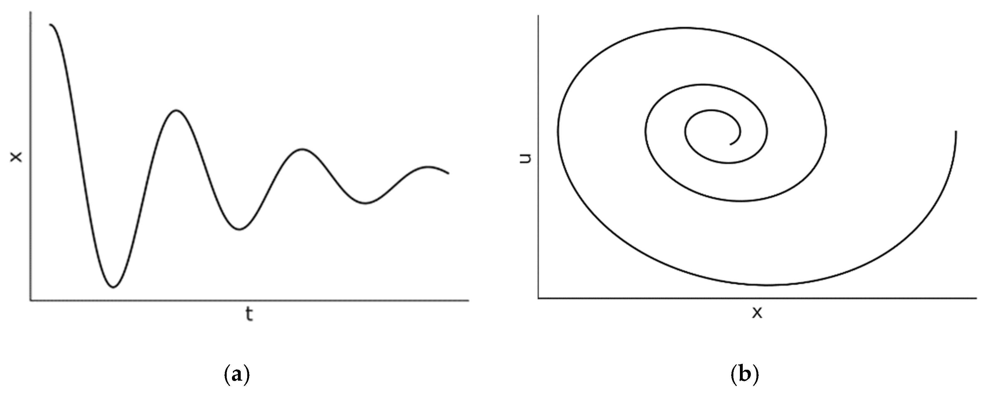
where . It is easy to see that Equation (6) is very similar to the underdamped case . The key differences are that the frequency is smaller and there is an overall exponential damping term . The motion is a damped sinusoidal oscillation as it is illustrated in Figure 3. Here, the oscillation amplitude decreases exponentially with a time constant . Using the initial conditions and , it can be easily seen that and .
3. Hamiltonian Mechanics and Poisson Brackets
Hamiltonian mechanics provides a geometric formulation of classical and quantum mechanics where the state of a system is described by canonical coordinates of position and momentum in phase space, where . The evolution of the system is governed by a scalar function , the Hamiltonian, which typically corresponds to the total mechanical energy. More generally, the Hamiltonian is defined as.
where is the kinetic energy and is the potential energy of the system. For any particle of mass in a potential , this becomes:
The equations of motion are given by Hamilton's equations:
These can be compactly expressed using the Poisson bracket , defined for any two functions and as:
The evolution of any observable is then given by:
This structure ensures that phase-space volume is preserved during evolution (Liouville's theorem), and that the Hamiltonian is conserved. In this sense, the Poisson bracket formalism not only generates the equations of motion but also encodes the geometric properties of conservative dynamics. However, this framework, applies strictly to conservative systems. Dissipative systems, such as those involving friction or damping, fall outside this traditional scope since energy is dissipated and entropy is produced. To describe irreversible processes, a more general framework is needed—one that incorporates both reversible (Hamiltonian) and irreversible (dissipative) dynamics in a consistent way, such the GENERIC framework or Quantitative Geometrical Thermodynamics (QGT).
4. Irreversible Thermodynamics and Entropy Production
In a damped harmonic oscillator, the total mechanical energy (the sum of kinetic and potential energy) is not conserved due to the energy being dissipated as heat or another form of energy through the damping mechanism. The instantaneous mechanical energy is given by:
The energy dissipation rate is derived by taking the time derivative of :
Using the equation of motion (Equation 1):
Substitute into Equation (13):
This energy is dissipated as heat into the environment, implying entropy production. If the surrounding reservoir is at constant temperature , the rate of entropy production is:
Using the definition of momentum , the rate of entropy production for the damped harmonic oscillator can be written as:
This irreversible entropy generation is incompatible with standard Hamiltonian mechanics, which assumes zero entropy production. Among the first attempts to unify conservative and dissipative dynamics was the GENERIC framework (General Equation for Non-Equilibrium Reversible-Irreversible Coupling), which extends the phase space to include both energy and entropy. In GENERIC, the state of the system is described by a set of variables (which now includes position, momentum, and entropy), and evolves according to the equation [26,27,30]:
Here, is the total energy functional, is the total entropy functional, is the Poisson operator, which is antisymmetric and encodes reversible dynamics, and is the dissipative operator, which is symmetric, positive semi-definite, and encodes irreversibility. The GENERIC structure ensures that:
- (entropy is not affected by reversible dynamics);
- (energy is not affected by dissipative dynamics);
By analogy with Hamiltonian mechanics where the evolution of any observable can be calculated using the Poisson brackets (Equation 10), it is equivalent for to write:
where
and
GENERIC framework imposes mathematical and physical constraints to ensure thermodynamic consistency. This theoretical structure can elegantly embed the irreversible thermodynamics of a dissipative system, such as the damped oscillator within a generalized Hamiltonian formalism, thereby enabling a consistent description of entropy production and conservative mechanics in a unified framework.
5. Quantitative Geometrical Thermodynamics (QGT)
As discussed in the Introduction, in QGT the physical time is defined as a complex dynamical variable. Instead of treating the imaginary parameter as isomorphic to the real-time variable , is defined as the analytic continuation into the complex plane as:
That is, the real and imaginary components of the complex time are explicitly distinguished, such that and appear independent of each other.
Following the introduction of the complex time , Velazquez, Parker and Jeynes introduce the concept of action-entropy as a holomorphic function of the classical action and the thermodynamic entropy across complex time (see Equations 16 and 17), which explicitly combines action and entropy as follows [19]:
where the Boltzmann constant and is reduced Planck constant (). It is obvious from Equation (23) that is dimensionless. Since is holomorphic, Cauchy–Riemann equations are valid as:
Using the conventional definition of the Hamiltonian , which is related to dissipationless (reversible) processes and the entropy production (or from Equations 16 and 17), related to dissipative (irreversible) processes, it is derived:
In Equation (26), is the associated with reversible processes, while is associated with irreversible processes.
When a function is holomorphic and the Cauchy-Riemann equations are satisfied, differentiating across the complex plane z is given by the Wirtinger operator as:
In this way, the complex differential of the actio-entropy is evaluated as:
It should be emphasized that represents the real (reversible) part of the complex Hamiltonian (the subscript indicates the relation of the variable to the complex time ), while is regarded as the real (irreversible) part of the complex entropy production . The nature of any physical process, as described by the complex Hamiltonian and the complex entropy production , depends on the trajectory the system follows through complex time. Specifically, the reversibility or irreversibility of the process (or any combination thereof) is determined by the combination of the real and imaginary components at each moment.
Within the framework of the temporal complex plane , its counterpart (complex-conjugated) complex frequency plane is introduced as:
In this manner, the Fourier transform for the conjugate frequencies of the respective real and imaginary temporal components are defined:
Equation (31) shows that both time and frequency are respectively analytically continued into their complex planes, with the complex time and complex frequency representing the appropriate conjugate pair, . For the case of the function being causal (i.e., for , where is chosen as a convenient point in time to express the causality of the system) and also physically realizable (square-integrable) function, then Cauchy’s theorem applies. This means that the Hamiltonian is holomorphic in the required (upper, as appropriate) half-plane, such that it obeys the dispersion relations (best known as practical constraints in signal processing). John Toll [31] gives rigorous proof that strict causality is logically equivalent to the existence of dispersion relations. Specifically, he shows that the real and imaginary properties of the dispersion are mutually related via the Kramers–Kronig relations, using the properties of the Hilbert transform. Following Toll ‘s [31] Equation (2.5), the dispersion of the complex Hamiltonian (Equation 28) using the component of the complex frequency is written as:
where is the principal part to be taken at the point . It should be noted that because the real and imaginary parts of are Hilbert transforms of each other, they are indeed causal. Similarly, the dispersion of the complex entropy production (Equation 29) using the component of the complex frequency is written as:
Again, is the principal part to be taken at the point . It is also noteworthy that applying the Hilbert transform to the negative temporal direction of the irreversible -axis reverses the conventional cause-and-effect relationship observed in the forward time direction. In other words, along the irreversible -axis, from the viewpoint of normal (forward-moving) time, the order of events is reversed: the "effect" precedes the "cause."
Using the mathematical properties of analytical continuation, one may write two symmetrical pairs of expressions for how the complex entropy production function and the complex Hamiltonian function relate along the two conjugate frequency axes forming the complex frequency plane:
Using the Cauchy–Riemann equations (Equations 24-25), it is now possible to relate the entropy production values on the real frequency -axis to the appropriate Hamiltonian values on the imaginary frequency -axis.
Using the formulation above, and can be evaluated as:
In general, and are evaluated as:
Finally, in a slightly more compact form, and are related as:
The relevant (cross-axial) components of the complex Hamiltonian and entropy production in Equations (28-29) are also simplified as:
6. Entropy Production and Hamiltonian of the Underdamped Harmonic Oscillator Using QGT
As discussed above, for conservative systems like an undamped harmonic oscillator, the Hamiltonian represents the system's total energy and remains constant over time. On the other hand, damping introduces energy dissipation, which implies breaking time-reversal symmetry, making the system non-conservative. In such cases, the Hamiltonian is not given straightforwardly. Based on these, QGT can be employed to explore the dynamics of a DHO and perhaps derive a Hamiltonian from its entropy production. It should be noted that Parker and Jeynes [31] derived an analytic relation for the entropy production of a DHO using McDonald’s [31] Hamiltonian approach. Here, the opposite process is followed, where a Hamiltonian is derived from entropy production as it is given from irreversible thermodynamics.
As a start, the simplest case of the DHO will be considered, i.e., the underdamped oscillator where . The position of this oscillator as a function of time is given by Equation (6). Using generic boundary conditions and , Equation (6) is written as:
while the velocity is calculated as:
where and .
Averaging over one period (see Appendix A), the total energy decays exponentially:
where equal to total mechanical energy of the undamped oscillator. Using Equation (55), is calculated as:
In this manner, using Equation (16) is derived as:
Following the steps of Parker and Jeynes [15], the Fourier transform of is calculated using Equation (31) to determine its real and imaginary frequency components as:
where, without loss of generality, it is considered that for . From Equation (58), it is evident that the complex entropy production has real and imaginary frequency components:
Similar to the Hamiltonian frequency components for the DHO in the paper of Parker and Jeynes [15], the two components of Equation (58) are also Hilbert transforms of each other, as causality requires. Using Equation (29) while including an additional instance of frequency to maintain correct dimensionality, it is derived that:
From Equations (39) and (42), it derived that:
Using Equations (62) and (63), it is concluded:
From Equation (45), the complex entropy production associated with an underdamped oscillator is written as follows:
Equation (65) can be further simplified using the concept of relaxation time, i.e., the time needed for the underdamped oscillator to dissipate all its energy, which in this case is (see §2.3). As stated by Córdoba et al. [32], any nonstationary system thermalizes to its final equilibrium state in time of the order of Boltzmann time . It is possible to identify the oscillator’s mechanical relaxation time with Boltzmann time due to the fact that the oscillator is immersed in a thermal reservoir at temperature and the damping is interpreted as arising from quantum–thermal dissipation (i.e., ). In this manner, relating the relaxation time of the underdamped oscillator with Boltzmann time, it is derived that:
It should be noted that Parker and Jeynes [15] derived a similar relation for temperature (see Equation 36 in their paper). Inserting Equation (66) into Eq. (65), the complex entropy production in now evaluated as:
while and are calculated as:
Using Equations. (40) and (41), and are derived from and as follows:
Inserting Equations (68)-(69) in Equations (70)-(71), it is concluded that:
From Equation (44), is written as:
It is evident from Equations (67) and (74) that as it is predicted from QGT (see Equation 50). Moreover, Equations (72) and (73) are similar to Equation (32) from the paper of Parker and Jeynes [15]. Finally, the real Hamiltonian can be now derived using the inverse Fourier transform as:
where the additional instance of frequency is now subtracted. It is evident that Equation (75) is identical to the Equation (9) of McDonald's paper. In addition to McDonald's methodology for deriving Hamiltonian formulation for dissipative systems, such as the DHO, the real Hamiltonian of the underdamped harmonic oscillator can be also predicted as a Wick-rotated complex conjugate of the entropy production using QGT. In this manner, the entropy production, as well as the Hamiltonian for the general solution of a DHO (a solution valid in all cases), will be calculated using QGT in the next section.
7. Entropy Production and Hamiltonian of the General Form of the DHO Using QGT
As can be seen from §2, a DHO is distinguished into three cases depending on the value of . Fortunately, these cases can be written in a closed form using a general solution that is valid in all the parameter ranges and initial conditions (see Equation 3). In this manner, the square of the velocity (see Equation 4) is calculated as follows:
Using the definition of entropy production (Equation 16), the latter for the general form of the DHO is derived as:
Following the steps from §6, the Fourier transform of is calculated using Eq. (31) to determine its real and imaginary frequency components as:
where, for simplicity, it is considered that for . From Equation (78), it is evident that the complex entropy production has real and imaginary frequency components:
Similarly to the entropy frequency components for the underdamped harmonic oscillator (Equations 59-60), the two components in Equations (79)-(80) are Hilbert transforms of each other, as causality requires. Using Equation (29) while including an additional instance of frequency to maintain correct dimensionality, it is derived that:
Using Equation (63) with Equation (82), it is concluded:
In this manner, the complex entropy production for the DHO is written as follows:
As in the case of the underdamped harmonic oscillator (see §6, Equation 84) can be further simplified using the concept of relaxation time, i.e., Equation (66):
while and are calculated as:
Using Equations (70) and (71), and are derived from and as follows:
From Equation (44), is written as:
As it was expected from the results of the underdamped oscillator, , a standard relation predicted from QGT (see Equation 50). Finally, the real Hamiltonian can be now derived using the inverse Fourier transform (Equation 75) as:
where the additional instance of frequency is now subtracted. Using that and , the real Hamiltonian can be written as:
which coincides with the instantaneous mechanical energy of the DHO multiplied by the factor . This result matches that of the underdamped harmonic oscillator, with the difference that the mechanical energy is not constant—an approach which was also adopted by Parker and Jeynes [15] in their own calculations. Furthermore, this result also coincides with McDonald's expression for the Hamiltonian of the DHO (see Equation 9 in his paper), again with the distinction that the mechanical energy does not remain constant. In this manner, the final expression for the Hamiltonian of the general solution of the DHO is written as:
To calculate the Poisson brackets for the underdamped harmonic oscillator, it is necessary to define the canonical momentum, also introduced by McDonald [29], rather than the mechanical momentum :
The canonical momentum ensures that the system can be cast into a Hamiltonian form with a well-defined Poisson bracket structure that satisfies Liouville's theorem. Physically, accounts for the energy loss introduced by the dissipative medium (in this case the heat bath), scaling the momentum to embed the irreversible effects into the phase-space evolution. Moreover, the Hamiltonian of the general solution of the DHO, derived using QGT (Equation 93) can be written in terms of the mechanical momentum and the canonical momentum :
In this manner, Hamilton's equations (Equation 9) are satisfied as:
By differentiating one more time and using Equations (94) and (96), the DHO differential equation of motion is recovered (Equation 1).
While the Hamiltonian formalism derived from QGT (see Equation 93) embeds dissipative dynamics into a reversible framework using complex time, the GENERIC framework separates the reversible and irreversible contributions by introducing an explicit entropy variable. To compare the two frameworks, the differential equation of motion will be derived for the DHO using GENERIC. In this manner, the state variable for the DHO is defined as where the entropy is also an independent variable along with the position and the momentum . The total energy is given as:
where is the internal energy of the system with:
The gradients of the energy and entropy with respect to the state variable are calculated as:
The Poisson operator depends only on and as:
Being antisymmetric, satisfies . Next, the dissipative operator should be defined. It is important for to contribute damping to , to preserve the total energy and to increase entropy. Moreover, must be symmetric, positive semidefinite and to satisfy . Due to these reasons, the final form of was determined as:
Using Equation (18), the final GENERIC structure for the DHO is written as:
The above equation results in the derivation of the known equations of motion for the DHO as:
The GENERIC structure for the DHO highlights entropy as thermodynamic potential. It also ensures that the second thermodynamics law holds, while the energy is conserved through .
8. Discussion
In this paper, a Hamiltonian formulation is derived for the damped harmonic oscillator, both for the underdamped case and for the general form that includes all damping cases. The Hamiltonian is formed using the Quantitative Geometrical Thermodynamics (QGT). This model is based on the complex time formalism which allows to reinterpret dissipation in classical systems through a unifying thermodynamic framework. By analytically continuing real time into the complex plane—where reversible dynamics evolve along the imaginary axis and irreversible processes along the real axis—one obtains a dual description of physical evolution in terms of energy (Hamiltonian) and entropy production. In this setting, the Hamiltonian of the system and its entropy production rate are not just analogous but mathematically isomorphic, connected through Hilbert transform that emerges from causality. Such a result reframes the classical energy–entropy relationship as a deeper geometrical equivalence in the complex temporal domain.
Τhe derivation of the Hamiltonian for the DHO from entropy production was successfully achieved through QGT, validating and extending the formalism proposed by Parker and Jeynes [15]. Notably, for the underdamped case, the entropy production rate was shown to yield a real Hamiltonian of the form matching McDonald’s relation (Equation 9) [29] when is the average mechanical energy over a period. Due to the oscillatory nature of this case, the averaging produces a constant mechanical energy, which justifies the exponential form of the Hamiltonian. This confirms that dissipation, encoded in entropy production, can be Wick-rotated to reconstruct a valid Hamiltonian for systems with weak damping, where weak oscillations dominate.
However, extending this analysis to the general DHO solution, valid across all damping regimes, reveals a key distinction: the mechanical energy is no longer constant but evolves explicitly in time, leading to a time-dependent Hamiltonian. Despite this, the formal structure of the Hamiltonian remains similar to the underdamped case, preserving the exponential factor and satisfying the same causality and Hilbert transform conditions prescribed by QGT. This verifies that QGT is not limited to near-conservative or weakly dissipative systems, but is robust enough to derive well-defined Hamiltonians even for systems characterized by strong thermodynamic irreversibility, such as the critically damped and overdamped harmonic oscillators. Therefore, the generalized Hamiltonian derived from QGT not only recovers McDonald's formulation [29] but unifies the regimes by embedding the entropy production directly into the Hamiltonian.
In general, the results of this work carry significant implications for our understanding of time asymmetry in dissipative systems. Classical mechanics, when formulated through conventional Hamiltonian dynamics, is inherently time-reversible; yet real-world systems ubiquitously exhibit irreversible behavior. By embedding entropy production directly into the Hamiltonian structure through the complexification of time, QGT offers a unified and elegant framework in which the arrow of time emerges not as an external constraint, but as an intrinsic geometric feature of the system’s evolution. The appearance of imaginary energy components—manifesting as entropy production—demonstrate that the asymmetry between past and future is encoded within the analytic structure of the actio-entropy function itself. In this view, time irreversibility is not merely a statistical artifact but a fundamental consequence of the holomorphic extension of classical dynamics. Thus, the QGT formalism not only combines energy dissipation with Hamiltonian mechanics but also deepens our conceptual grasp of the origins of temporal directionality in physical systems.
An additional insight emerging from the QGT-derived Hamiltonian for the DHO is its compatibility with a generalized Poisson bracket structure, despite the presence of dissipation. Traditionally, Poisson brackets encode the symplectic geometry of conservative systems, where the Hamiltonian preserves phase-space volume (Liouville's theorem). However, the exponential factor found in the QGT-derived Hamiltonian, derived from the entropy production, explicitly breaks time-reversal symmetry and induces phase-space conservation. Notably, by defining the canonical momentum in a manner similar to McDonald's formulation [29] one can retain a modified, yet meaningful Poisson bracket structure. In this formulation, the time evolution of the variables remains governed by Hamilton’s equations, but now includes irreversible dynamics through the QGT Hamiltonian. Thus, the results of this paper enable the embedding of thermodynamically consistent dissipation into the framework of classical mechanics, laying a foundation for extension into metriplectic and GENERIC formulations that systematically unify reversible and irreversible dynamics.
A natural extension of this work lies in comparing the QGT-derived Hamiltonian structure with the GENERIC (General Equation for the Non-Equilibrium Reversible-Irreversible Coupling) framework. GENERIC provides a geometric structure that combines a Poisson bracket (antisymmetric) for reversible dynamics and a dissipative bracket (symmetric and positive semi-definite) for irreversible dynamics. In this setting, the state vector comprising position, momentum, and entropy—evolves according to the coupled flow equations generated by both the Hamiltonian and entropy. While QGT embeds dissipation through the complexification of time and derives a single effective Hamiltonian containing both reversible and irreversible content, GENERIC maintains a dual-generator structure where the Hamiltonian governs the reversible part and the entropy governs the irreversible. Yet, both approaches reveal an intimate link between entropy production and the time evolution of the dissipative system.
Crucially, the QGT-derived Hamiltonian for the DHO integrates entropy production implicitly through its time dependence, matching the GENERIC requirement that the total energy is not conserved in the presence of entropy increase. While GENERIC preserves the explicit separation of structure via the and matrices (antisymmetric and symmetric, respectively), QGT internalizes these features into the analytic structure of the complexified Hamiltonian and its causal properties. Importantly, both frameworks converge on a consistent thermodynamic interpretation: entropy production is directly tied to irreversible evolution, whether captured as an explicit generator (in GENERIC) or as an imaginary energy component (in QGT). Therefore, the QGT result provides a minimal, unified Hamiltonian description of dissipation that enriches the more structured, bracket-based GENERIC approach.
Finally, it is important to note the isomorphism between the imaginary component of the complex time and the antisymmetric Poisson matrix through the lens of geometric algebra (see Appendix B). The imaginary component of complex time in QGT, responsible for reversible dynamics, plays the same structural role as the antisymmetric Poisson matrix in GENERIC. Both define infinitesimal generators of rotation, preserve a conserved quantity (energy), and act on their respective spaces (complexified time and phase space) to produce reversible, unitary evolution. This correspondence allows us to interpret and as isomorphic in geometric algebra, suggesting that QGT’s complex geometry is a natural complexification of the real-valued symplectic geometry of conventional Hamiltonian mechanics. In this view, entropy production arises from the breakdown of symmetry between these two geometrical structures — the real axis in QGT and the dissipative metric bracket in GENERIC.
9. Conclusions and future Directions
In this work, it is demonstrated that a Hamiltonian relation for the damped harmonic oscillator (DHO) can be rigorously derived from entropy production using the framework of Quantitative Geometrical Thermodynamics (QGT). By treating time as a complex variable and interpreting entropy production as the imaginary component of energy, a unified Hamiltonian structure is recovered that remains valid across all damping regimes. This formulation not only reproduces the known results of McDonald's Hamiltonian and Parker and Jeynes [15,29] for the underdamped oscillator but also extends to critically and overdamped cases, embedding the full dissipative character of the system within a causally consistent, complex-analytic framework. The QGT-derived Hamiltonian was shown to preserve a generalized Poisson structure, while the imaginary time component seems to be isomorphic to the antisymmetric Poisson operator in GENERIC, which shows the deeper connection between entropy, energy, and complex time.
The implications of these findings extend well beyond the scope of the DHO. First, the ability of QGT to encode irreversible thermodynamics in a single complex Hamiltonian suggests that similar approaches could be fruitfully applied to a broader class of dissipative systems, including the Navier–Stokes equations, reaction–diffusion systems, and viscoelastic media. Moreover, the geometric isomorphism between the imaginary time component and the Poisson matrix, as revealed through geometric algebra, opens a pathway to reinterpret classical mechanics in a holomorphic and geometrically unified formalism. Future work may explore how this framework interacts with spacetime algebra, providing insights into the arrow of time and causality at a relativistic or even cosmological scale. In quantum mechanics, the complex time approach may offer new routes to reconcile unitary evolution with decoherence and information loss, with potential connections to the thermodynamics of measurement, quantum entropy production, and Von Neumann entropy. Finally, the connection between energy and entropy production within complex time presents intriguing opportunities for advancing information theory, geometric thermodynamics, and classical mechanics, ultimately enriching our understanding of both microscopic and macroscopic irreversibility from a unified geometric standpoint.
Funding
This research received no external funding.
Institutional Review Board Statement
Not applicable.
Data Availability Statement
The data presented in this study are available on request from the corresponding author.
Acknowledgments
The author would like to thank Dr. Chris Jeynes for fruitful discussions regarding QGT and the nature of time.
Appendix A
Here a general proof for the time-averaged energy over one oscillation for the underdamped harmonic oscillator is shown. The general solution for the position can be written as (in addition to the form that is shown in Equation 53):
where phase constant and is the initial amplitude. The time derivative of equals to the velocity as:
The square of the velocity is given as:
The instantaneous total energy is given by Equation (12). Since oscillates rapidly due to the and terms, it is useful to consider its time average over one period. This means that the and terms are averaged as:
In this manner, the time-averaged kinetic energy is calculated as:
and the time-averaged potential energy is calculated as:
The total averaged mechanical energy is now derived as:
Using that (see §2.3), is written as:
where . Equation (10) shows that the time-averaged mechanical energy for the underdamped harmonic oscillator decays exponentially with initial energy equal to total mechanical energy of the undamped harmonic oscillator.
Appendix B
In this Appendix, the isomorphism between the unit antisymmetric matrix and the bivector in Geometric Algebra (GA) will be shown. A real antisymmetric matrix satisfies:
which leads to the form:
This matrix has one degree of freedom and its determinant is equal to one (). The square of this matrix is calculated as:
where is the unit matrix. This shows that the unit antisymmetric matrix can rotate any vector in by 90°.
In geometric algebra of the wedge product of two orthonormal basis vectors and defines the unit bivector [33,34]:
The bivector behaves algebraically like the imaginary unit from complex numbers with . The wedge product defines an oriented area and is antisymmetric as [35]:
Now consider the action of the matrix on a vector . This yields:
This is exactly a counterclockwise rotation by 90°, which is also the effect of multiplying the complex number by as:
which is written in vector form:
This corresponds to the action of matrix , which highlights the duality between bivectors in geometric algebra and antisymmetric matrices in linear algebra.
It is concluded that the unit antisymmetric matrix is the real matrix representation of the bivector in geometric algebra, and corresponds to multiplication by the imaginary unit in the complex plane. It encodes a 90° rotation and satisfies , just like .
References
- Mita, K. Schrödinger's equation as a diffusion equation. Am. J. Phys. 2021, 89, 500–510. [Google Scholar] [CrossRef]
- Callender, C. Measures, Explanations and the Past: Should ‘Special’ Initial Conditions be Explained? Brit. J. Philos. Sci. 2004, 55, 195–217. [Google Scholar] [CrossRef]
- Lebowitz, J.L. Boltzmann's Entropy and Time's Arrow. Phys. Today 1993, 46, 32–38. [Google Scholar] [CrossRef]
- Riek, R. Entropy Derived from Causality. Entropy 2020, 22. [Google Scholar] [CrossRef] [PubMed]
- Rovelli, C. White Holes; Random House: New York, USA, 2023. [Google Scholar]
- Seifert, U. Stochastic thermodynamics, fluctuation theorems and molecular machines. Rep. Prog. Phys. 2012, 75, 126001. [Google Scholar] [CrossRef] [PubMed]
- Prigogine, I. Time, Structure, and Fluctuations. Science 1978, 201, 777–785. [Google Scholar] [CrossRef] [PubMed]
- Prigogine, I.; Hiebert, E.N. From Being to Becoming: Time and Complexity in the Physical Sciences. Phys. Today 1982, 35, 69–70. [Google Scholar] [CrossRef]
- Kapusta, J.I.; Gale, C. Finite-Temperature Field Theory: Principles and Applications, 2nd ed.; Cambridge University Press: Cambridge, 2006. [Google Scholar]
- Wick, G.C. Properties of Bethe-Salpeter Wave Functions. Phys. Rev. 1954, 96, 1124–1134. [Google Scholar] [CrossRef]
- Callan, C.G.; Coleman, S. Fate of the false vacuum. II. First quantum corrections. Phys. Rev. D 1977, 16, 1762–1768. [Google Scholar] [CrossRef]
- Hartle, J.B.; Hawking, S.W. Wave function of the Universe. Phys. Rev. D 1983, 28, 2960–2975. [Google Scholar] [CrossRef]
- Hawking, S.W. Arrow of time in cosmology. Phys. Rev. D 1985, 32, 2489–2495. [Google Scholar] [CrossRef] [PubMed]
- Hawking, S.W. Particle creation by black holes. Commun. Math. Phys. 1975, 43, 199–220. [Google Scholar] [CrossRef]
- Parker, M.C.; Jeynes, C. Relating a System’s Hamiltonian to Its Entropy Production Using a Complex Time Approach. Entropy 2023, 25, 629. [Google Scholar] [CrossRef] [PubMed]
- Parker, M.C.; Jeynes, C. Maximum entropy (most likely) double helical and double logarithmic spiral trajectories in space-time. Sci. Rep. 2019, 9, 10779. [Google Scholar] [CrossRef] [PubMed]
- Parker, M.C.; Jeynes, C. Entropic uncertainty principle, partition function and holographic principle derived from Liouville’s Theorem. Phys. Open 2021, 7, 100068. [Google Scholar] [CrossRef]
- Parker, M.C.; Jeynes, C.; Walker, S.D. A Metric for the Entropic Purpose of a System. Entropy 2025, 27, 131. [Google Scholar] [CrossRef] [PubMed]
- Velazquez, L.; Parker, M.; Jeynes, C. The Geometry of Thermodynamics III. 2022. [CrossRef]
- Kaufman, A.N. Dissipative hamiltonian systems: A unifying principle. Phys. Lett. A 1984, 100, 419–422. [Google Scholar] [CrossRef]
- Morrison, P.J. A paradigm for joined Hamiltonian and dissipative systems. Phys. D: Nonlinear Phenom. 1986, 18, 410–419. [Google Scholar] [CrossRef]
- Arnol'd, V.I. Mathematical methods of classical mechanics; Springer Science & Business Media, 2013; Volume 60. [Google Scholar]
- Gay-Balmaz, F.; Yoshimura, H. A Lagrangian variational formulation for nonequilibrium thermodynamics. Part I: Discrete systems. J. Geom. Phys. 2017, 111, 169–193. [Google Scholar] [CrossRef]
- Sanders, J.W.; DeVoria, A.C.; Washuta, N.J.; Elamin, G.A.; Skenes, K.L.; Berlinghieri, J.C. A canonical Hamiltonian formulation of the Navier–Stokes problem. J. Fluid Mech. 2024, 984, A27. [Google Scholar] [CrossRef]
- De Groot, S.R.; Mazur, P. Non-equilibrium thermodynamics; Courier Corporation, 2013. [Google Scholar]
- Lebon, G.; Jou, D.; Casas-Vázquez, J. Understanding non-equilibrium thermodynamics; Springer, 2008; Volume 295. [Google Scholar]
- Öttinger, H.C. Beyond equilibrium thermodynamics; John Wiley & Sons, 2005. [Google Scholar]
- Chandrasekar, V.K.; Senthilvelan, M.; Lakshmanan, M. On the Lagrangian and Hamiltonian description of the damped linear harmonic oscillator. J. Math. Phys. 2007, 48, 032701. [Google Scholar] [CrossRef]
- McDonald, K.T. A damped oscillator as a Hamiltonian system. Available online: http://kirkmcd.princeton.edu/examples/damped.pdf (accessed on 29/03/2025).
- Öttinger, H.C. GENERIC integrators: structure preserving time integration for thermodynamic systems. J. Non-Equilib. Thermodyn. 2018, 43, 89–100. [Google Scholar] [CrossRef]
- Toll, J.S. Causality and the dispersion relation: logical foundations. Phys. Rev. 1956, 104, 1760. [Google Scholar] [CrossRef]
- Fernández de Córdoba, P.; Isidro, J.M.; Vázquez Molina, J. Schroedinger vs. Navier–Stokes. Entropy 2016, 18, 34. [Google Scholar] [CrossRef]
- Hestenes, D. Spacetime physics with geometric algebra. Am. J. Phys. 2003, 71, 691–714. [Google Scholar] [CrossRef]
- Hestenes, D.; Lasenby, A. Space-time algebra; Springer, 2015. [Google Scholar]
- Hestenes, D. Vectors, spinors, and complex numbers in classical and quantum physics. Am. J. Phys. 1971, 39. [Google Scholar] [CrossRef]
Figure 1.
The (a) position-time dependence and (b) state-space diagrams (right side) for the overdamped harmonic oscillator where . In Figure 1b, the velocity is denoted by .
Figure 1.
The (a) position-time dependence and (b) state-space diagrams (right side) for the overdamped harmonic oscillator where . In Figure 1b, the velocity is denoted by .
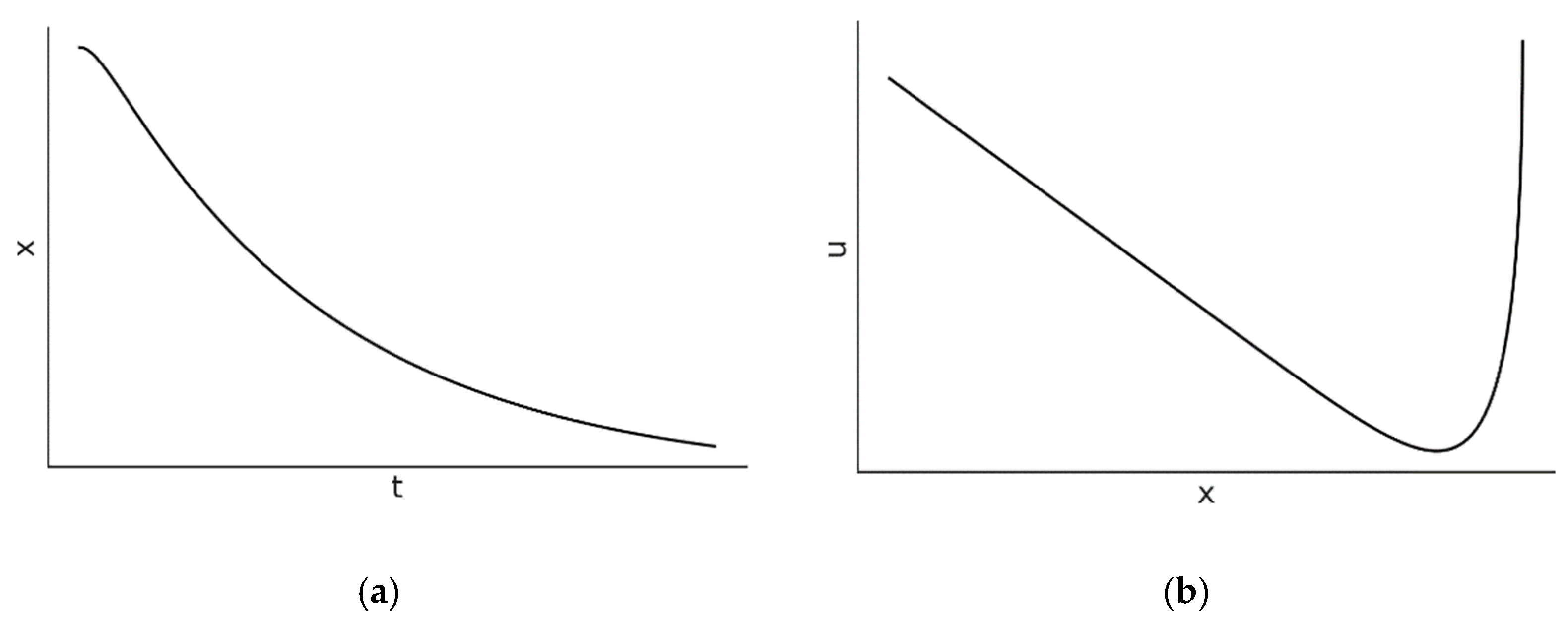
Figure 2.
The (a) position-time dependence and (b) state-space diagrams (right side) for the critically damped harmonic oscillator where . In Figure 2b, the velocity is denoted by .
Figure 2.
The (a) position-time dependence and (b) state-space diagrams (right side) for the critically damped harmonic oscillator where . In Figure 2b, the velocity is denoted by .
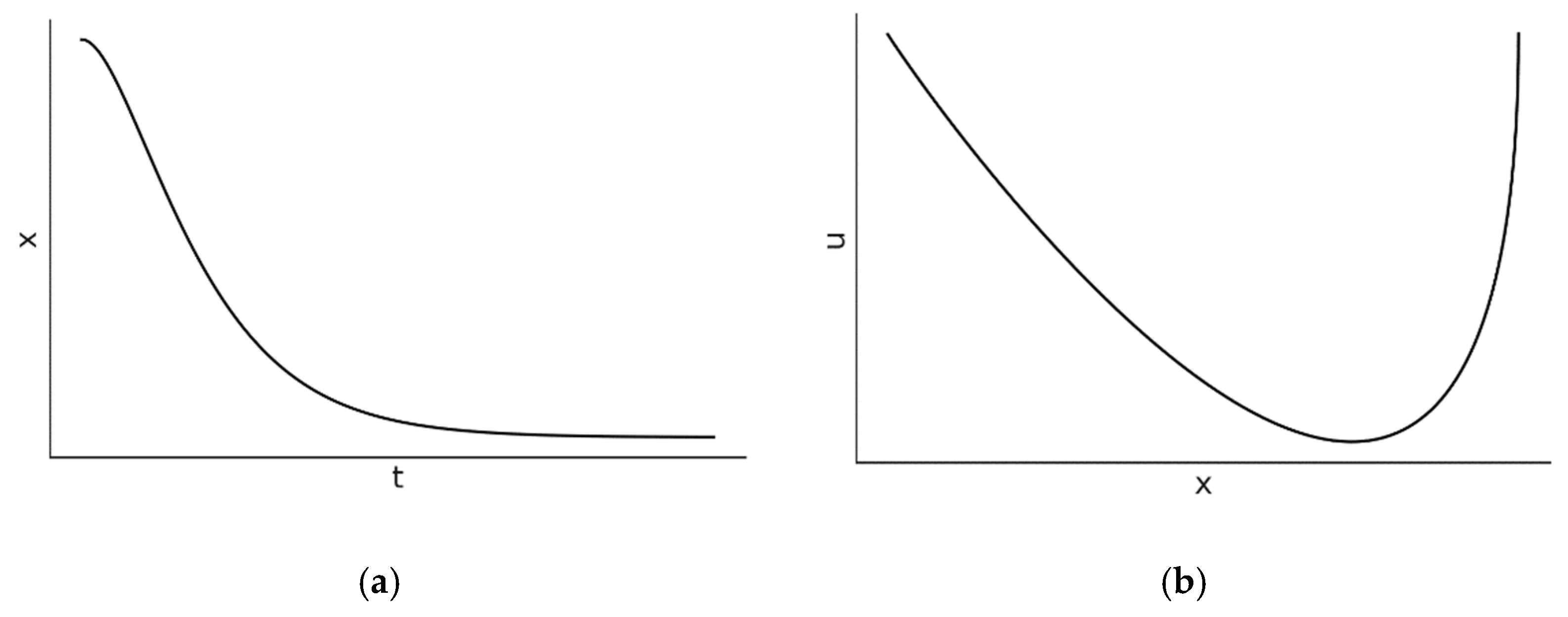
Figure 3.
The (a) position-time dependence and (b) state-space diagrams (right side) for the underdamped harmonic oscillator where . In Figure 3b, the velocity is denoted by .
Figure 3.
The (a) position-time dependence and (b) state-space diagrams (right side) for the underdamped harmonic oscillator where . In Figure 3b, the velocity is denoted by .
Disclaimer/Publisher’s Note: The statements, opinions and data contained in all publications are solely those of the individual author(s) and contributor(s) and not of MDPI and/or the editor(s). MDPI and/or the editor(s) disclaim responsibility for any injury to people or property resulting from any ideas, methods, instructions or products referred to in the content. |
© 2025 by the authors. Licensee MDPI, Basel, Switzerland. This article is an open access article distributed under the terms and conditions of the Creative Commons Attribution (CC BY) license (http://creativecommons.org/licenses/by/4.0/).
Copyright: This open access article is published under a Creative Commons CC BY 4.0 license, which permit the free download, distribution, and reuse, provided that the author and preprint are cited in any reuse.


