
Submitted:
28 April 2025
Posted:
29 April 2025
You are already at the latest version
Abstract
Quantifying methane (CH₄) emissions is essential for climate change mitigation, yet current estimation methods often suffer from substantial uncertainties, particularly at the site level. This study introduces a drone-based approach for measuring CH₄ emissions using an open-path Tunable Diode Laser Absorption Spectroscopy (TDLAS) sen-sor mounted parallel to the ground, rather than in the traditional nadir-pointing con-figuration. Controlled CH₄ release experiments were conducted to evaluate the method’s accuracy, employing a modified mass balance technique to estimate emission rates. Two wind data processing strategies were compared: a logarithmic wind profile (LW) and a constant scalar wind speed (SW). The LW approach yielded highly accurate results, with an average recovery rate of 98%, while the SW approach showed greater variability with increasing distance from the source, though remained reliable in close proximity. The method demonstrated the ability to quantify emissions as low as 0.08 g s⁻¹ with approximately 5% error, given sufficient sampling. These findings suggest that the proposed UAV-based system is a promising, cost-effective tool for ac-curate CH₄ emission quantification in sectors such as agriculture, energy, and waste management, where traditional monitoring techniques may be impractical or limited.
Keywords:
methane emission
; drone-based monitoring
; open-path TDLAS
; mass-balance approach
1. Introduction
The reduction of anthropogenic methane emissions is one of the most effective strategies to rapidly curb the rate of global-warming and significantly contribute to limiting global temperature rise. Methane (CH₄) is in fact a powerful greenhouse gas, with a global warming potential 86 times greater than that of CO₂ over a 20-year period, and 30 times greater over a 100-year timescale [1].
Anthropogenic methane emissions are responsible for nearly half of the observed global warming since pre-industrial levels and account for 60% of the total methane released into the atmosphere. Over the past two centuries, the Earth’s average temperature has increased by 1.2°C, largely due to human-caused emissions [2].
The main sources of anthropogenic methane emissions are attributable to agriculture and livestock (enteric fermentation, manure management, rice cultivation), the energy sector (extraction, storage, transport and use of fossil fuels), and the waste sector (landfill disposal, wastewater treatment). In 2021, agriculture was the leading source of anthropogenic emissions (42%), followed by energy (38%) and waste (20%) [2].
Quantifying methane emissions into the atmosphere from these three sectors is usually approached through either bottom-up or top-down methodologies, and the validation of emission inventories requires both. Bottom-up methods use activity data (amount of waste produced or disposed of, number of livestock, facility components, energy consumption, etc.) multiplied by standardised emission factors. Top-down approaches, on the other hand, rely on direct measurements (usually aerial or satellite) of atmospheric CH₄ concentrations, from which emission rates are derived using dispersion models.
Despite its significant impact as a greenhouse gas, current estimates of CH₄ emissions are characterised by high uncertainty across all sectors, and there is rarely good agreement between the two inventory types.
Several studies have highlighted a substantial underestimation by bottom-up methodologies when compared with direct field (top-down) measurements, concluding that many bottom-up inventories are likely not representative of actual atmospheric methane emissions [3,4,5,6,7].
A recent study compared bottom-up estimates of an agricultural area in Ontario with aerial measurements and various emission quantification methods [8]. The top-down estimates showed good agreement among themselves but exceeded the bottom-up figures by 117%.
In the energy sector, emissions from a natural gas extraction facility were estimated using satellite measurements and compared with bottom-up inventories, revealing values up to seven times higher [9].
To quantify emissions from coal mines in Queensland (Australia's largest coal-producing state) satellite measurements were carried out over two years [10]. The resulting estimates were significantly higher than those reported in the Australian government’s bottom-up inventories.Methane emissions from landfill waste disposal and wastewater treatment also show a marked discrepancy between bottom-up and top-down estimates, with the former often significantly lower [11,12].
The reasons for this divergence remain unclear. Some studies point out that emission factors are based on datasets from the 1990s and are thus potentially outdated [13,14]; others suggest that the underestimation may stem from bottom-up inventories failing to account for emissions released during abnormal conditions or equipment malfunctions [13,15,16].
Additionally, uncertainties remain in the quantification methods and technologies used for top-down estimates. It is therefore important to continue and expand top-down studies to enhance understanding of the divergence between the two inventory types across the three sectors [17].
Quantifying methane emissions requires measuring the molar fraction of the gas in the atmosphere in combination with wind measurements (speed and direction). CH₄ concentrations can be estimated using ground-based, aerial or satellite systems. Ground-based systems may include fixed stations [18,19], mobile units operated manually [20,21,22], or vehicle-mounted platforms [23,24,25,26].
Ground-based systems allow for direct measurement of emissions close to the surface and can eliminate interference from surrounding sources, but these methods are often time-consuming and require complex interpolation techniques. Vehicle-based surveys can reduce the duration of data collection; however, they require accessible road infrastructure, which is not always available, thereby limiting their applicability in certain environments. Moreover, these surveys often encounter challenges in accurately locating and distinguishing individual emission points [27,28].
Aerial monitoring is widely used to quantify CH₄ emissions over large areas, such as cities or wetlands [29,30,31]. However, conventional research aircraft are often too large and lack the manoeuvrability required to estimate emissions from small local sources such as landfills or fossil fuel facilities [32].
Several solutions employ smaller, more manoeuvrable aircraft to estimate small-scale anthropogenic methane emissions, but the quantification methods used require a stable background and minimal external influences [33,34,35].
Satellite measurements have greatly aided in identifying methane super-emitters, but the technology is not yet mature enough to estimate CH₄ emissions at small scales. Satellite systems can struggle in mountainous terrain, snow- or ice-covered regions, and at high latitudes. They are also affected by cloud cover, even partial, limiting the number of usable observation days and making them poorly suited to comparison with bottom-up inventories [36].
Unmanned Aerial Vehicles (UAVs, or drones) offer new opportunities to quantify CH₄ fluxes from various facility types, thanks in part to advances in sensor miniaturisation, which has made instruments lighter and suitable for drone deployment.
Compared with crewed aerial monitoring, drones can sample air closer to the surface, providing information otherwise inaccessible by aircraft. Their high manoeuvrability, fewer flight restrictions, and the relatively low cost of many sensors have driven rapid adoption of UAV-based systems across sectors, from agriculture to energy and waste management [37,38].
For atmospheric CH₄ monitoring, drones are often equipped with closed-path TDLAS (Tunable Diode Laser Absorption Spectroscopy) sensors. These instruments take point measurements along horizontal transects at different altitudes on the downwind side of a site. The data are then interpolated and combined with wind measurements to estimate emission rates via a mass balance approach.Numerous studies have implemented this in practice, for example to estimate CH₄ emissions from livestock [39], coal mines [40,41], and solid waste landfills [42,43,44].
Sampling density is crucial for obtaining reliable results but may require long and impractical survey times. As a result, the spacing between successive transects is often around 10 m, which can introduce significant uncertainty in the data interpolation.
Additionally, measurements must be taken at a sufficient distance from the site to ensure adequate plume mixing and representative point measurements. However, increasing distance requires higher-sensitivity sensors (on the order of ppb) which are more expensive, and makes it harder to separate external contributions in flux estimation.
An alternative solution involves using an open-path TDLAS sensor, which may improve the representativeness of spatial interpolation by providing integrated CH₄ concentrations along an optical path and eliminating the need to reconstruct data distribution along the beam direction.
This study proposes a UAV-based approach to estimate CH₄ emissions from various site types and discusses the results of controlled release tests. It differs from the experiments conducted by [45,46] in the orientation of the optical path, which is not nadir-pointing but horizontal.
The methodological approach is similar to that of [47], with comparable spatial test scales. However, it differs in the use of a drone and a non-fixed, drone-mounted sensor.
This paper is structured as follows. Section 2 describes the proposed method and test design in detail. Results are analysed and discussed in Section 3, with a focus on measured concentrations (Section 3.1) and their spatial distribution (Section 3.2). Emission fluxes are then derived using two distinct wind data processing methods (Section 3.3). The influence of key parameters on results is discussed in Section 3.4. Section 4 concludes the study, summarising the strengths and limitations of the proposed approach, suggesting potential solutions, and identifying aspects warranting further investigation.
2. Materials and Methods
This section outlines the methods and tools used in the present study. Section 2.1 introduces the UAV platform, and the sensors required for the application of the method. Section 2.2 briefly summarises the adopted mass balance approach. Finally, Section 2.3 describes the experimental configurations of the controlled release tests.
2.1. UAV Platform and Instrumentation
The UAV platform used is a commercial quadcopter (Matrice 350, DJI), equipped with a Real-Time Kinematic (RTK) system for high-precision positioning. Typically, spatial coordinates are obtained using GPS (Global Positioning System) data combined with on-board atmospheric pressure measurements, particularly to determine flight altitude. However, this method generally provides vertical accuracy within several tens of centimetres, which is not sufficient to quantify gas fluxes with the required precision [52]. The RTK system used by the M350 drone allows for positioning accuracy of 1.5 cm (± 1 ppm) vertically and 1 cm (± 1 ppm) horizontally.
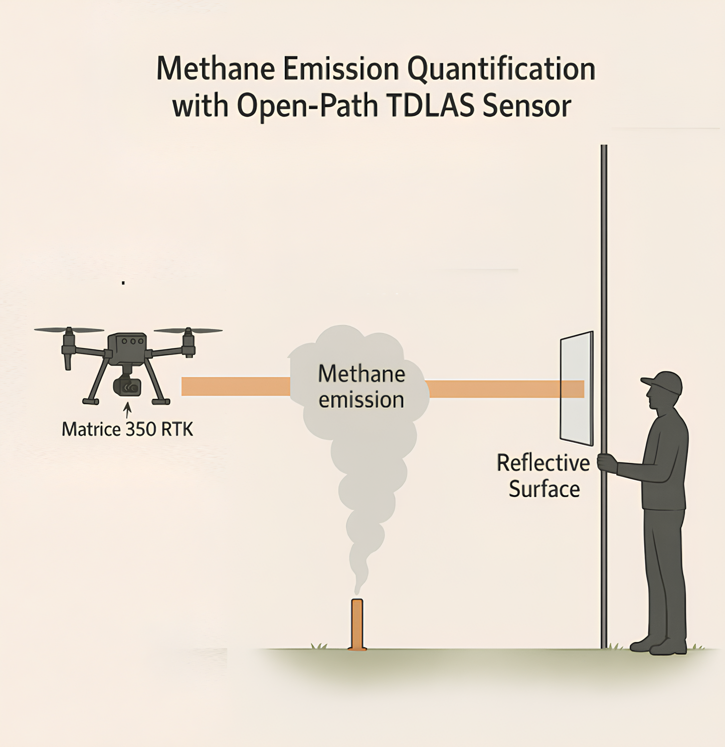
The UAV platform is fitted with an open-path Tunable Diode Laser Absorption Spectroscopy (OP-TDLAS) methane spectrometer. The sensor (Laser Falcon methane detector, Pergam-Suisse AG) emits electromagnetic radiation at a wavelength selective for CH₄ (1.65 μm); this beam reaches a designated target (typically the ground) and is then reflected back to the sensor. The intensity of the return signal is proportional to the CH₄ concentration along the optical path (in accordance with the Beer-Lambert law). The device records data at a frequency of 10 Hz and provides measurements expressed in ppm-m (range: 0–50,000 ppm-m). The support brackets were customised to allow horizontal mounting of the sensor. Thus, the laser is not oriented nadirally towards the ground but rather directed at a vertical target – a pole-mounted, mobile retro-reflective panel.
The retro-reflective panel measures 50 cm x 50 cm and is attached to a 9-metre pole, along which it can be raised using a pulley system. The maximum height of the pole was determined as a compromise between operational constraints and data from the literature. [47,48] observed measurable CH₄ increases at no more than 6–7 metres above ground level under comparable conditions in terms of the spatial scale of the measurements.
The design of the retro-reflective panel was optimised to enhance pointing precision and accuracy. The drone is equipped with a zoom camera and a viewfinder to maintain correct alignment with the target during flight. Any misalignment is identified and corrected during post-processing of the raw data, together with potential false positives from the OP-TDLAS sensor, using a dedicated algorithm [49].
False positives refer to erroneous readings indicating the presence of CH₄ when it is either absent or present in negligible amounts. These may arise from external interferences, calibration errors, or unfavourable environmental conditions. False positives can lead to incorrect conclusions and negatively impact the precision and reliability of measurements. Therefore, regular calibration checks and the development of dedicated algorithms are essential to minimise the occurrence of false positives.
Meteorological parameters (wind speed and direction, temperature, atmospheric pressure) were recorded at 2 metres above ground level using a weather station positioned near the retro-reflective panel.
2.2. Mass-Balance Approach
The methodology proposed in this study is based on a Lagrangian approach to mass balance, which has previously been employed to estimate fugitive CH₄ emissions from various landfill sites through airborne measurements [34] or UAV platforms [42,50,51].
It differs in the type of concentration measured and processed, which is not a point value but rather represents the total amount of CH₄ along a horizontally measured optical path (g m⁻²).
The UAV system described in Section 2.1 directs the horizontal laser beam towards a retro-reflective panel, performing rapid successive scans at different heights. The maximum distance from the panel depends on the technical specifications of the OP-TDLAS sensor mounted on the drone. The sensor used in this study can detect CH₄ over an optical path of up to 100 m. However, the manufacturer recommends an optical path length between 30 and 50 m to optimise performance. Therefore, the tests were carried out using a 50 m optical path.
Since the OP-TDLAS sensor allows for the calculation of an integrated concentration along an optical path (g m⁻²), the CH₄ flux for the i-th vertical scan, Fᵢ (g s⁻¹), can be estimated using Equation (1):
where (m s-1) is the horizontal wind component at altitude z (m), θ is the angle between the wind direction and the optical path, and represents the increase in the integrated CH₄ concentration relative to the background level along the same path (g m⁻²). The subscript d indicates that the measurement was taken downwind of the source, b refers to the background concentration, z denotes the altitude of the optical path, and i identifies the i-th vertical scan.
The final emission rate F (g s⁻¹) is calculated as the average over n scans conducted during a single flight (Equation 2):
The duration of a flight depends on the number of scans performed, as well as the drone’s altitude and vertical speed. Experimental observations have shown that a minimum of four scans is sufficient to obtain satisfactory results. Assuming an altitude of 9 m and a vertical speed of 1 m s⁻¹, the time required to complete four scans is approximately 36 seconds.
When comparing our approach with that of a drone equipped with a point sensor, each single scan across a plane downwind of the source typically takes longer to complete (approximately 50 seconds). As a result, spatial resolution is compromised in favour of faster scanning, but this complicates subsequent data interpolation and reduces accuracy (particularly in the vertical direction). Furthermore, non-simultaneous sampling along the vertical axis of the plume is one of the main limiting factors in achieving accurate emission estimates using the mass balance approach [39]. In Figure 1, the flight plan is shown with the transects covered by the drone during the survey.
2.2.1. Conversion from ppm-m to Integrated Concentration (g m⁻²)
The integrated mole fractions returned by the sensor (ppm-m) were converted into an integrated concentration (g m⁻²) using equation (3), which approximates the behaviour of CH₄ as an ideal gas:
where the terms P, T, and R respectively represent atmospheric pressure, temperature, and the universal gas constant, while 16.04 (g mol⁻¹) is the molecular weight of CH₄. The mole fraction of water vapour (H₂O, %) is calculated based on temperature and relative humidity (RH) measurements. In cases where humidity is not measured during the survey, the (1 – H₂O) contribution may be omitted from equation (3). The uncertainty introduced by humidity is, in fact, less than 1% [52]. Since the focus is solely on CH₄ concentration increase above the background level, this error can be considered minor and negligible in the absence of field measurements.
2.2.2. CH4 Background Measurements
The background concentrations (CH₄,b) were measured by conducting upwind flights relative to the emission source, carried out a few minutes prior to the quantification flight. The same experimental setup was adopted (maintaining the same distance from the retroreflective panel and scanning height). The results were then processed statistically to remove any false positives. The validated measurements were divided by the actual lengths of the optical paths and subsequently averaged, yielding an average background CH₄ concentration expressed in ppmv.
Assuming an approximately constant background level across the vertical plane, the integrated CH₄,b concentration along each path was calculated as the product of the average value and the optical path length.
2.2.3. Wind Measurements
The wind speed perpendicular to the generic optical path was estimated using two different approaches. The first method is based on the construction of a theoretical logarithmic wind profile, which has already been adopted by several UAV-based methodologies in landfills [53,54] and in various controlled release tests [52,55].
Based on the parameters measured by the meteorological station at a height of 2 m, the wind speed v(z,i) (m s⁻¹) at a given height z (m) is calculated using equation 4:
where (m s-1) is the wind speed measured at the reference height zr (2m), z₀ represents the surface roughness of the terrain (m), while Ψm is a correction function depending on atmospheric stability. The term L represents the Monin-Obukhov length, which defines the ratio between the convective and mechanical forcing of turbulence.
The second approach is conceptually simpler. Each sensor measurement was associated with the instantaneous wind data recorded by the meteorological station at 2 m above ground level. It is assumed that the station is near the measurement plane, in order to minimise the uncertainty due to spatial variability of the wind field and turbulent transport.
2.3. Controlled Release Test
The controlled release tests were conducted in an open field cultivated with grass. The site morphology is approximately flat, and there are no potential external sources of CH4 nearby. The grass height was less than 5 cm, and there are were obstructions to wind flow within the field. However, the site is bordered by high-speed roads on two sides. To exclude possible interference from turbulent phenomena induced by vehicular traffic, a safety zone was defined. This limitation allowed the vertical plane to be placed no more than 20 m from the source.
A total of 22 tests were conducted between 15 and 17 January 2024, of which 20 were suitable for flux quantification. During the last two flights on 17 January, the meteorological station failed to record data due to technical issues, and the flights were discarded. The main operational parameters of the valid tests are summarised in Table 1.
The days selected for the tests presented favourable meteorological conditions, with winds exceeding 1 m s-1 and no precipitation. The source consisted of a cylinder containing CH4 (99%), equipped with a flow meter and connected by a small tube (internal diameter 1.2 cm) to the release point. The end of the tube was positioned approximately 10 cm above the surface to simulate a ground emission. Each release lasted on average 20 seconds, and the vertical plane was measured at various distances from the source (1 m, 10 m, 20 m).
The release rates were selected based on the minimum emission estimated using the chamber method across 11 US landfills (Abichou et al., 2011). The 428 tests conducted between May 2006 and December 2009 provided an emission rate ranging from 0.06 g s-1 to 2.00 g s-1.
To verify that the CH4 released during one test did not interfere with the measurements of the next, screening flights were conducted at the end of each test. For this purpose, a second drone was used, equipped with a multi-gas sensor (Sniffer 4D, range 0–10000 ppm, resolution 1 ppm). The subsequent release was carried out only when the concentrations measured within the study area fell within the ambient background range.
3. Results and Discussion
This section summarises and discusses the results obtained from the experimental tests. The statistical distributions of CH4 concentrations are analysed in section 3.1, along with their vertical profiles in section 3.2. Section 3.3 describes and compares the CH4 fluxes obtained from the two methodological assumptions tested. Finally, section 3.4 examines the impact of the two approaches on the result.
3.1. CH4 Concentration Measurements
Figure 2 shows the distribution of the average CH4 increments relative to the background concentration for the 20 valid tests, aggregated based on the distance from the emission point. The average values are obtained by dividing each measurement by the length of the respective optical path. A clear decrease in average ppm values is evident as the distance from the source increases. The value quickly drops from 40.6 ppm at 1 m (Figure 2a) to 4.7 ppm at 10 m (Figure 2b) and then further decreases to 0.96 ppm at 20 m (Figure 2c). Similarly, the maximum concentration observed at 1 m from the source (966 ppm) reduces by 70% at 10 m and by 98% at 20 m. This represents a clear expression of the dispersion phenomenon and transport mechanisms. It also confirms the ability of the proposed methodology to capture emissions during the controlled release tests.
A particular feature of the open-path TDLAS sensor is that its sensitivity depends on the optical path length. Provided that the return signal strength is adequate to ensure measurement reliability and that the recorded value exceeds the background noise, the Laser Falcon can detect the presence of CH4 when the total concentration along the optical path reaches a minimum value of 1 ppm-m. The optical path length in the tests conducted was about 50 m, which corresponds to a sensitivity of 0.02 ppmv.
As is well known, the horizontal dispersion of the plume is more pronounced than the vertical dispersion during transport, although the impact depends on atmospheric stability. This aspect compromises the spatial resolution of the sensor when mounted on a drone in a nadir position and limits the detection of CH4 emissions around 0.011 g s-1 to within 10 m of the source [45,46].
To increase the signal-to-noise ratio, it is necessary to detect high concentrations of CH4 above the background level. Flying at low altitude would be optimal, but turbulence induced by the downwash of the propellers may yield unreliable results [48], 2021; Kim et al., 2021).
Orienting the optical path horizontally allows for exploiting the transverse dispersion and keeping the readings above the instrument’s detection threshold for greater distances from the emission point compared to the nadir configuration. As a result, it was possible to fully capture CH4 increments above the background concentration even at more than 10 m from the source (Figure 2c).
To understand how the orientation of the optical path affects spatial resolution, tests were conducted using a Lagrangian particle model in both configurations (horizontal and vertical configurations). The aim was to quantify the capture percentage at increasing downwind distances (from 1 m to 50 m) for a CH4 emission point at ground level with a rate of 0.050 g s-1. The simulations were carried out under neutral atmospheric stability conditions, on a flat, obstacle-free surface cultivated with grass (surface roughness 2 cm), with various wind speeds (from 1 to 5 m s-1).
A downwind plane, perpendicular to the wind direction, was defined, with dimensions of 50 m x 10 m, centred on the emission point. The plane was scanned by several linear sensors to measure integrated concentrations along the optical path (ppm-m), with a step of 10 cm for the vertical configuration and 2 cm for the horizontal configuration.
At the end of each simulation, the measured integrated concentrations were compared to those exceeding 1 ppm-m (the sensitivity of the instrument). The test was then repeated by increasing the wind speed up to 5 m s-1, followed by increasing the distance from the source by one metre and repeating the procedure until reaching 50 m. The limit distance was defined based on the sensor's ability to fully capture the plume.
The results are shown in Figure 3 for the vertical configuration and in Figure 4 for the horizontal configuration.
As expected, spatial resolution worsens with increasing wind speed in both cases. When the OP-TDLAS sensor is positioned in a nadir orientation relative to the ground, the maximum detection distance rapidly decreases with wind speed (35 m at 2 m s-1, 20 m at 3 m s-1, 15 m at 4 m s-1, and 10 m at 5 m s-1). At 50 m with a wind speed of 1 m s-1, the system detects only 50% of the total emission.
The horizontal orientation of the sensor allows for significantly better recovery, managing to capture 30% of the emission at 50 m from the source when the wind is 5 m s-1 and 95% when the wind is 1 m s-1.
These results were derived assuming neutral atmospheric stability conditions; therefore, it is expected that capture percentages and maximum detection distances will tend to increase with higher stability classes and worsen in unstable conditions.
Additionally, the mathematical model operates under steady-state assumptions. With a constant wind of 1 m s-1, an emission takes 50 seconds to travel 50 m. Due to atmospheric turbulence, it is unlikely that there will be no changes in speed and/or direction during this time interval. This suggests that the actual curves may be characterised by steeper slopes or may result in a combination of the curves represented in Figure 3 and Figure 4. This deviation is expected to increase with flight time, being minimal near the source and maximum at 50 m with weak winds (1 m s-1).
3.2. Vertical Distribution of Average CH4 Concentrations
The extent of the plume depends on its distance from the emission point and atmospheric stability. Under stable conditions, convective motions are strongly inhibited, favouring the horizontal transport of the gas along the mean wind direction. This tends to keep the emission plume low during transport. As instability increases, convective contributions become more significant, leading to a marked predominance of vertical motions, which contributes to more crosswise dispersion of the gas at higher altitudes than in the longitudinal direction.
Figure 5 shows the vertical profiles of CH4 increments for the 20 tests conducted, once again divided based on the downwind distance from the emission point. The results near the source (1 m) highlight average horizontal transport below 4 m. The concentrations show a slight decreasing trend with height, reaching the peak at 1.57 m (966 ppm) and the minimum at 4.16 m (5.43 ppm).
Even at 10 m from the emission point, the horizontal transport dissipates within 4 m of the ground, but the decreasing trend is less pronounced due to the increased turbulent dispersion in the atmosphere caused by the distance.
Tests conducted at 20 m suggest CH4 increments beyond the maximum measured height (8.5 m), and the peak concentration is observed at 4.72 m above the ground.
It is likely that the height of the retroreflector was insufficient to fully capture the plume at this distance, or the number of averaging repetitions (4 for each flight) was not adequate to define a representative plume morphology.
The results are consistent with those obtained by [47], who conducted several controlled CH4 release tests under similar conditions. Compared to the maximum detection distance of 30 m estimated by the authors, the study conducted here limits the distance to 20 m downwind for estimating a CH4 flux with 50 m optical paths.
Since the source position was central to the measurement plane in both studies, it would be beneficial to increase the horizontal extent of the window by conducting more measurements and integrating the measured data. For instance, the window could be extended to 100 m and the measurement could be split into two separate planes (0-50 m and 50-100 m), estimating the total CH4 flux as the sum of the two contributions.
For practical reasons, it will be quite difficult to extend the measurement heights beyond 10 m. This obstacle could be overcome by using two synchronised drones in a simultaneous flight, with the first carrying the OP-TDLAS sensor and the second carrying the retroreflector panel and following the movements of the first drone.
The use of a drone equipped with a retroreflector panel has already been observed in literature [56,57], although in these studies the detector is fixed on the ground. There are significant regulatory restrictions regarding flying, which currently make the development and management of a simultaneous flight with multiple drones quite impractical.
3.3. Emission Estimates
The CH4 fluxes (g s-1) estimated for each test are summarised in Table 2, differentiated by the approach used for processing the wind data (scalar wind SW and logarithmic wind LW) (Table 2).
Both approaches show a good degree of agreement with the actual emission; however, the assumption of a logarithmic wind profile appears to be more robust than the scalar one. In fact, this method exhibits lower mean absolute errors (1.9-10.3%) compared to the use of scalar wind (2.3-37.8%), with a tendency for the error to increase as the downwind distance from the release point grows.
These results suggest that the logarithmic wind-based approach could be more accurate.In the SW approach, the mean absolute error also tends to increase with distance from the source, but the trend is less clear, and errors of a similar magnitude can be observed both 1 metre downwind (test 9: 36.9%; test 10: 20.8%; test 15: 17.4%) and at 20 m (test 7: 23.2%; test 13: 28.4%; test 14: 37.8%).
When using an atmospheric mass balance to estimate the methane flux in the atmosphere, the wind vector is a key parameter, and it accounts for much of the total uncertainty in the estimate, along with the variability of the background concentration during the flight [42].
It is therefore important to estimate the wind field with sufficient accuracy, in order to associate each concentration measurement with the wind speed that best approximates the actual value. The error is also amplified near the source due to poor vertical mixing of the plume. This results in a high variability in CH4 concentrations, which risks not being captured and could compromise the representativeness of the result.
The LW approach tends to slightly underestimate the actual emitted flux (Figure 6). The only exception is represented by tests 19 and 20, conducted 10 m from the source under weak wind conditions. These circumstances do not favour adequate transport of the emitted gas, which tends to stagnate and is therefore repeatedly detected by the sensor. The SW approach does not exhibit a clear trend; the CH4 flux was both overestimated (8 tests) and underestimated (12 tests). In tests 7, 9, 10, 13, and 14, the overestimation exceeded 20% of the actual emission rate, and almost all of these measurements were taken 20 m downwind.
Figure 7 summarises the capture efficiencies of the two tested approaches. The LW approach shows a constant average efficiency (around 98%), regardless of distance. In contrast, the use of scalar wind overestimates at 1 m (103%) and at 20 m (120%), while it tends to underestimate at 10 m (94%).
The results are consistent with those obtained by [52], who highlighted a mean error using scalar wind that was 4% higher than that of logarithmic wind under optimal conditions.
Ultimately, the assumption of a logarithmic wind profile has proven to be a more robust approach than the use of scalar wind. While the former captured the emission with minimal deviation (2%) from the actual flux, the latter is affected by the turbulent fluctuations typical of transport phenomena, resulting in larger errors. The reduced standard deviation is attributable to the speed of the measurement, which allows for four scans to be completed in less than 40 seconds (which is not able to capture the stochastic variability of the emission profile).
Finally, it is noted that the capture percentages for the LW approach are perfectly comparable to those shown in Figure 5, which report efficiencies ranging from 95% to 100% for distances less than 20 m, with winds between 1 and 2 m s-1 (conditions of the field tests).
3.4. Optimal Conditions
The experimental data were further analysed using a DOE (Design of Experiment) approach. This term refers to a design and analysis technique that involves the intentional manipulation of one or more process factors to study their effect on measurable responses.
The method allows for detailed information to be gathered on the cause-and-effect relationships between variables and helps to identify the optimal conditions to either maximise or minimise a given response. DOE thus provides a statistical and scientific approach to making decisions based on experimental data, offering a solid foundation for process optimisation and the search for innovative solutions. It is widely used in various sectors, from pharmaceutical design to water treatment [58,59,60].
In this study, two process variables (wind speed and distance from the source) were identified, with the aim of understanding their effect on the response variable (mean percentage error). Other available process variables (mean concentration of ambient background, standard deviation of wind speed, angle between the plane and the wind vector) were excluded as they were statistically insignificant (p value > 0.05).
The low standard deviation observed in wind speed is likely due to the speed of the measurement, which was completed in about 40 seconds per flight (too short to capture the variability induced by atmospheric turbulence). More interesting is the non-significance of the angle between the plane and the wind direction. This is due to both the speed of the measurement and the flexibility of the panel equipped with a retroreflector. Unlike fixed systems (which require initial collimation and must remain stationary to maintain alignment with the sensor), the designed panel can be easily rotated by the operator. This allows for the panel to be positioned perpendicular to the wind direction just moments before the flight, reducing random effects induced by turbulence over time.
Figure 8 illustrates the trend of the mean percentage error for the LW approach. Near the source (d < 3 m) with weak winds (< 1.2 m s-1), the underestimation is at its maximum (< 8%). This is likely due to the portion of the plane not scanned by the drone (from 0 to about 0.5 m). The drone automatically initiates the landing protocol when it is at a short distance from the ground. To address this issue, it was necessary to maintain a minimum altitude during the scans, which left a dark zone in the first vertical segment. It is possible that the plume was not fully captured during some tests, as also indicated by Figure 5.
As the distance from the source increases, the error tends to decrease without showing a clear dependence on wind speed. In the range of 14 - 18 m and for winds below 1.6 m s-1, the best match is observed, and the method starts to slightly overestimate the actual flux (< 2%). As the distance increases and for winds below 1.3 m s-1, the overestimation exceeds 2%.
The SW approach (Figure 9) is characterised by higher mean percentage errors, and the graph is consistent with what was already observed in the previous section. Near the source (d < 2 m), the method slightly overestimates the actual emission (up to 10%). As the distance increases, there is a tendency to underestimate by up to 10%, with no apparent relationship to wind speed. From 15 m onwards, the trend reverses, with vertical areas showing increasing overestimation up to 20 m (> 40%).
4. Conclusions
This study presents and discusses the results of 22 controlled CH4 release tests conducted between 15 and 17 January 2024 at a test field cultivated with grass. The objective was to estimate the emission rate on a downwind plane at various distances from the source, using an UAV-based mass balance. A quadcopter drone (M350, DJI) was used, equipped with a TDLAS sensor with an open path to measure integrated CH4 concentrations. Wind data were collected from a ground-based weather station. Two different approaches for processing the wind data were tested: assuming a logarithmic wind profile (LW) with height or using the wind data from the weather station as constant and representative over the entire plane (SW).
The main results can be summarised in the following points:
- The recoveries calculated using the LW approach were on average 98%, regardless of the downwind distance from the source.
- The recoveries calculated using the SW approach showed more variable trends with distance, with good correspondence near the source (102%) and marked overestimation at 20 m from the source (120%).
- Experimentally, it was observed that a minimum of 4 scans was sufficient for the LW approach, while it is recommended to increase this number for the SW approach in order to reduce the plume variability induced by atmospheric turbulence.
- Due to the short time required to perform 4 scans (about 40 seconds) and the manoeuvrability of the retroreflector panel, it was easy to ensure the perpendicularity of the plane to the wind during each test. Therefore, wind direction variability was negligible.
- The results were consistent with numerical simulations carried out using a Lagrangian particle model for pollutant dispersion in the atmosphere, considering two different scenarios: one with a horizontal path and the other with a vertical path for the laser sensor.
The study demonstrated that the proposed technique can identify an emission rate of at least 0.08 g s-1 within 5% of the actual value using the LW approach, provided that the number of scans is sufficient (at least 4).
Several limitations and aspects requiring further study were also identified. In particular, the height of the plane is limited by the operational practicality of the retroreflector system (which can hardly exceed 10 m in the field).
An ideal configuration would involve the simultaneous and synchronised flight of two drones, but this is currently strongly constrained by existing flight regulations (procedural complications for issuing permits, waiting times, and higher costs). Alternatively, gas-filled balloons, building walls or industrial sheds could be used to lift the retroreflector panel, as they are considered to be similar to masts under many regulations up to 50 m in height and do not require specific permits. However, this reduces the system's flexibility and adds costs and management complications for transporting and storing the gas to be used.
Another aspect to consider is the maximum length of the optical path. The laser sensor used in this study allows measurement along an optical path up to 50 m, enabling the scanning of a plane with approximate dimensions of 50 m x 9 m. Since the plume disperses and the cross-section increases with distance, a wider scanning window is necessary.
Furthermore, the position of the source is often unknown. Therefore, it is preferable to scan larger planes by subdividing them into 50 m long tracks, estimating the emission as the sum of the contributions.
Finally, CH4 increments above the ambient background tend to decrease with distance from the emission point. It would be preferable to measure the ambient background concurrently with the release, rather than at previous or subsequent times. This aspect could be addressed in future experiments.
In conclusion, the proposed and analysed method is a promising tool for estimating CH4 emissions from various sectors (agriculture, energy, and especially waste), where the field situation allows its use.
Author Contributions
Conceptualization, D.F.; methodology, D.F., M.D.M., B.N., P.A.R.; software, F.A., M.D.M.; validation, B.N., P.A.R. and D.F.; formal analysis, D.F., F.A.; data curation, D.F., F.A., B.N., P.A.R., M.D.M.; writing—original draft preparation, D.F.; writing—review and editing, D.F.; visualization, B.N., P.A.R., M.D.M.; supervision, B.N., P.A.R. All authors have read and agreed to the published version of the manuscript.
Funding
This research received no external funding.
Data Availability Statement
The raw data supporting the conclusions of this article will be made available by the authors on request
Conflicts of Interest
The authors declare no conflicts of interest.
References
- IPCC, 2021: Climate Change 2021: The Physical Science Basis. Contribution of Working Group I to the Sixth Assessment Report of the Intergovernmental Panel on Climate Change [Masson-Delmotte, V., P. Zhai, A. Pirani, S.L. Connors, C. Johnson D. and Heltzel R., “Methane emissions measurements of natural gas components using a utility terrain vehicle and portable methane quantification system”. Atmospheric Environment, Volume 144, 2016, Pages 1-7. ISSN 1352-2310. [CrossRef]
- IEA, 2023. World Energy Outlook 2023, IEA, Parigi https://www.iea.org/reports/world-Energy-Outlook-2023, Licenza: CC BY 4.0 (rapporto); CC BY NC SA 4.0 (Allegato A).
- Zavala-Araiza, D, et al. 2018. Methane emissions from oil and gas production sites in Alberta, Canada. Elem Sci Anth, 6: 27. [CrossRef]
- Chan E., Worthy D.E.J., Chan D., Ishizawa M., Moran M.D., Delcloo A., Vogel F., 2020. Eight-year estimates of methane emissions from oil and gas operations in western Canada are nearly twice those reported in inventories. Environ. Sci. Technol., 54, pp. 14899-14909.
- Cusworth, D.H., Bloom, A.A., Ma, S. et al., 2021. A Bayesian framework for deriving sector-based methane emissions from top-down fluxes. Commun Earth Environ 2, 242 (2021). [CrossRef]
- MacKay, K., Lavoie, M., Bourlon, E. et al. 2021. Methane emissions from upstream oil and gas production in Canada are underestimated. Sci Rep 11, 8041 (2021). [CrossRef]
- Olczak M., Piebalgs A., Balcombe P., 2023. A global review of methane policies reveals that only 13% of emissions are covered with unclear effectiveness. One Earth, Volume 6, Issue 5, Pages 519-535. ISSN 2590-3322. [CrossRef]
- Desjardins R.L., Worth D.E., Pattey E., VanderZaag A., Srinivasan R., Mauder M., Worthy D., Sweeney C., Metzger S., 2018. The challenge of reconciling bottom-up agricultural methane emissions inventories with top-down measurements. Agricultural and Forest Meteorology, Volume 248, Pages 48-59. ISSN 0168-1923. [CrossRef]
- Dubey L., Cooper J., Staffell I., Hawkes A., Balcombe P., 2023. Comparing satellite methane measurements to inventory estimates: A Canadian case study. Atmospheric Environment: X, Volume 17, 100198. ISSN 2590-1621. [CrossRef]
- Sadavarte P., Pandey S., Maasakkers J.D., Lorente A., Borsdorff T., Denier van der Gon H., Houweling S., Aben I., 2021. Methane Emissions from Superemitting Coal Mines in Australia Quantified Using TROPOMI Satellite Observations. Environmental Science & Technology 2021 55 (24), 16573-16580. [CrossRef]
- Yeşiller N., Hanson J.L., Manheim D.C., Newman S., Guha A., 2022. Assessment of methane emissions from a California landfill using concurrent experimental, inventory, and modeling approaches. Waste Management, Volume 154, Pages 146-159. ISSN 0956-053X. [CrossRef]
- Liu Y., Paris J.D., Vrekoussis M., Quéhé P.Y, Desservettaz M., Kushta J., Dubart F., Demetriou D., Bousquet P., Sciare J., 2023. Reconciling a national methane emission inventory with in-situ measurements. Science of The Total Environment, Volume 901, 165896. ISSN 0048-9697. [CrossRef]
- Brandt, A. R. Heath, G.A., Kort, E.A. O’Sullivan, F., Pétron, G., Jordaan, S.M., Tans, P., Wilcox, J., Gopstein, A.M., Arent, D., Wofsy, S., Brown, N.J., Bradley, R., Stucky, G.D., Eardley, D., Harriss, R., 2014. Methane leaks from North American natural gas systems. Science 343, 733–735. https://www.researchgate.net/publication/260211785.
- Heath, G., Warner, E., Steinberg, D., Brandt, A. R., 2015. Estimating U. S. Methane Emissions from the Natural Gas Supply Chain: Approaches, Uncertainties, Current Estimates, and Future Studies.
- Brandt, A.R., Heath, G.A., Coole, D. 2016. Methane Leaks from Natural Gas Systems Follow Extreme Distributions. Environ. Sci. Technol. [CrossRef]
- Alvarez, R. A., Zavala-Araiza D., Lyon, D.R., Allen, D.T., Barkley, Z.R., Brandt, A.R., Davis, K.J., Scott C. Herndon, S.C., Jacob, D.J., Karion, A., Kort, E.A., Lamb, B.K., Lauvaux, T., Maasakkers J. D., Marchese, A.J., Omara, M., Pacala, S. W., Peischl, J., Robinson, A.L., Shepson, P.B., Sweeney, C., Townsend-Small, A., Wofsy, S.C., Hamburg, S.P., 2018. Assessment of methane emissions from the U.S. oil and gas supply chain. Science. eaar7204 (2018). https://www.researchgate.net/publication/325916333_Assessment_of_methane_emissions_from_the_US_oil_and_gas_supply_chain.
- Zhang S., Ma J., Zhang X., Guo C., 2023. Atmospheric remote sensing for anthropogenic methane emissions: Applications and research opportunities. Science of The Total Environment, Volume 893, 164701. ISSN 0048-9697. [CrossRef]
- Shaw Jacob T., Allen G., Pitt J., Mead M.I., Purvis R.M., Dunmore R., Wilde S., Shah A., Barker P., Bateson P., Bacak A., Lewis A.C., Lowry D., Fisher R., Lanoisellé M., Ward R.S., 2019. A baseline of atmospheric greenhouse gases for prospective UK shale gas sites. Science of The Total Environment, Volume 684, Pages 1-13. ISSN 0048-9697. [CrossRef]
- Knox, S. H., and Coauthors, 2019. FLUXNET-CH4 Synthesis Activity: Objectives, Observations, and Future Directions. Bull. Amer. Meteor. Soc., 100, 2607–2632. [CrossRef]
- Wu T, Cheng J, Wang S, He H, Chen G, Xu H, Wu S., 2023. Hotspot Detection and Estimation of Methane Emissions from Landfill Final Cover. Atmosphere. 14(11):1598. [CrossRef]
- Gazola B., Mariano E., Mota Neto L.V., Rosolem C.A., 2024. Greenhouse gas and ammonia emissions from a maize-soybean rotation under no-till as affected by intercropping with forage grass and nitrogen fertilization. Agricultural and Forest Meteorology, Volume 345, 109855. ISSN 0168-1923. [CrossRef]
- Stadler C., Fusé V.S., Linares S., Guzmán S.A., Juliarena M.P., 2024. Accessible sampling methodologies to quantify the net methane emission from landfill cells. Atmospheric Pollution Research, Volume 15, Issue 3, 102011. ISSN 1309-1042. [CrossRef]
- Zazzeri G., Lowry D., Fisher R.E., France J.L., Lanoisellé M., Nisbet E.G., 2015. Plume mapping and isotopic characterisation of anthropogenic methane sources. Atmospheric Environment, Volume 110, Pages 151-162. ISSN 1352-2310. [CrossRef]
- Johnson M.R., Tyner D.R., Szekeres A.J., 2021. Blinded evaluation of airborne methane source detection using Bridger Photonics LiDAR. Remote Sensing of Environment, Volume 259, 2021,112418. ISSN 0034-4257. [CrossRef]
- Fischer J.C., Cooley D., Chamberlain S., Gaylord A., Griebenow C.J., Hamburg S.P., Salo J., Schumacher R., Theobald D., Ham J., 2017. Rapid, Vehicle-Based Identification of Location and Magnitude of Urban Natural Gas Pipeline Leaks. Environmental Science & Technology 51 (7), 4091-4099. [CrossRef]
- Lowry D., Fisher R.E., France J.L., Coleman M., Lanoisellé M., Zazzeri G., Nisbet E.G., Shaw Jacob T., Allen G., Pitt J., Ward R.S., 2020. Environmental baseline monitoring for shale gas development in the UK: Identification and geochemical characterisation of local source emissions of methane to atmosphere. Science of The Total Environment, Volume 708, 2020, 134600. ISSN 0048-9697. [CrossRef]
- Ayasse, A.K., Thorpe, A.K., Cusworth, D.H., Kort, E.A., Negron, A.G., Heckler, J., Asner, G., Duren, R.M., 2022. Methane remote sensing and emission quantification of offshore shallow water oil and gas platforms in the Gulf of Mexico. Environ. Res. Lett. 17. [CrossRef]
- Wang, M., Shi, W., Tang, J., 2011. Water property monitoring and assessment for China’s inland Lake Taihu from MODIS-Aqua measurements. Remote Sens. Environ. 115, 841–854. [CrossRef]
- O'Shea, S. J., Allen, G., Gallagher, M. W., Bower, K., Illingworth, S. M., Muller, J. B. A., Jones, B. T., Percival, C. J., Bauguitte, S. J.-B., Cain, M., Warwick, N., Quiquet, A., Skiba, U., Drewer, J., Dinsmore, K., Nisbet, E. G., Lowry, D., Fisher, R. E., France, J. L., Aurela, M., Lohila, A., Hayman, G., George, C., Clark, D. B., Manning, A. J., Friend, A. D., and Pyle, J.,2014. Methane and carbon dioxide fluxes and their regional scalability for the European Arctic wetlands during the MAMM project in summer 2012. Atmos. Chem. Phys., 14, 13159–13174. [CrossRef]
- Heimburger, AMF, et al, 2017. Assessing the optimized precision of the aircraft mass balance method for measurement of urban greenhouse gas emission rates through averaging. Elem Sci Anth, 5: 26. [CrossRef]
- Tong X., van Heuven S., Scheeren B., Kers B., Hutjes R., Chen H., 2023. Aircraft-Based AirCore Sampling for Estimates of N2O and CH4 Emissions. Environmental Science & Technology 57 (41), 15571-15579. [CrossRef]
- Shaw, J.T.; Shah, A., Han, Y; Allen, G. 2021. Methods for quantifying methane emissions using unmanned aerial vehicles: a review. Phil. Trans. R. Soc. A.3792020045020200450. [CrossRef]
- Lavoie T.N., Shepson P.B., Cambaliza M.O.L., Stirm B.H., Karion A., Sweeney C., Yacovitch T.I., Herndon S.C., Lan X., and Lyon D., 2015. Aircraft-Based Measurements of Point Source Methane Emissions in the Barnett Shale Basin. Environmental Science & Technology 49 (13), 7904-7913. [CrossRef]
- Gasbarra D., Toscano P., Famulari D., Finardi S., Di Tommasi P., Zaldei A., Carlucci P., Magliulo E., Gioli B., 2019. Locating and quantifying multiple landfills methane emissions using aircraft data. Environmental Pollution, Volume 254, Part B, 112987. ISSN 0269-7491. [CrossRef]
- Kunkel W.M., Carre-Burritt A.E., Aivazian G.S., Snow N.C., Harris J.T., Mueller T.S., Roos P.A., and Thorpe M.J., 2023. Extension of Methane Emission Rate Distribution for Permian Basin Oil and Gas Production Infrastructure by Aerial LiDAR. Environmental Science & Technology 57 (33), 12234-12241. [CrossRef]
- Gaudioso D., 2022. Le emissioni di metano in Italia - Stime di emissione e priorità di intervento per la loro riduzione – giugno 2022. https://www.wwf.it/cosa-facciamo/pubblicazioni/le-emissioni-di-metano-initalia/.
- Fosco, D., De Molfetta, M., Renzulli, P., & Notarnicola, B., 2024. Progress in monitoring methane emissions from landfills using drones: an overview of the last ten years. Science of The Total Environment, 945, 173981. [CrossRef]
- Yao, H.; Qin, R.; Chen, X. 2019. Unmanned Aerial Vehicle for Remote Sensing Applications—A Review. Remote Sens., 11, 1443. [CrossRef]
- Vinković K., Andersen T., de Vries M., Bert Kers B., van Heuven S., Peters W., Hensen A., van den Bulk P., Chen H., 2022. Evaluating the use of an Unmanned Aerial Vehicle (UAV)-based active AirCore system to quantify methane emissions from dairy cows. Science of The Total Environment, Volume 831, 154898. ISSN 0048-9697. [CrossRef]
- Andersen, T.; Vinkovic, K.; de Vries, M.; Kers, B.; Necki, J.; Swolkien, J.; Roiger, A.; Peters, W.; Chen, H. 2021. Quantifying methane emissions from coal mining ventilation shafts using an unmanned aerial vehicle (UAV)-based active AirCore system, Atmospheric Environment: X, Volume 12, 100135, ISSN 2590-1621. [CrossRef]
- Andersen, T., Zhao, Z., de Vries, M., Necki, J., Swolkien, J., Menoud, M., Röckmann, T., Roiger, A., Fix, A., Peters, W., and Chen, H., 2023. Local-to-regional methane emissions from the Upper Silesian Coal Basin (USCB) quantified using UAV-based atmospheric measurements, Atmos. Chem. Phys., 23, 5191–5216. [CrossRef]
- Allen G., Hollingsworth P., Kabbabe K., Pitt J.R., Mead M.I., Illingworth S., Roberts G., Bourn M., Shallcross D.E., Percival C.J., 2019. The development and trial of an unmanned aerial system for the measurement of methane flux from landfill and greenhouse gas emission hotspots. Waste Management, Volume 87, Pages 883-892, ISSN 0956-053X. [CrossRef]
- Ali N.B.H., Abichou T. and Green R., 2020. Comparing estimates of fugitive landfill methane emissions using inverse plume modeling obtained with Surface Emission Monitoring (SEM), Drone Emission Monitoring (DEM), and Downwind Plume Emission Monitoring (DWPEM). Journal of the Air & Waste Management Association, 70:4, 410-424. [CrossRef]
- Yong, H.; Allen, G.; Mcquilkin, J.; Ricketts, H.; Shaw, J.T., 2024. Lessons learned from a UAV survey and methane emissions calculation at a UK landfill. Waste Management, Volume 180, Pages 47-54. ISSN 0956-053X. [CrossRef]
- Yang, S., Talbot, R.W., Frish, M.B., Golston, L.M., Aubut, N.F., Zondlo, M.A., Gretencord, C., McSpiritt, J., 2018. Natural Gas Fugitive Leak Detection Using an Unmanned Aerial Vehicle: Measurement System Description and Mass Balance Approach. Atmosphere, Volume 9, 383. [CrossRef]
- Golston, L.M.; Aubut, N.F.; Frish, M.B.; Yang, S.; Talbot, R.W.; Gretencord, C.; McSpiritt, J.; Zondlo, M.A., 2018. Natural Gas Fugitive Leak Detection Using an Unmanned Aerial Vehicle: Localization and Quantification of Emission. Rate. Atmosphere 9, 333. [CrossRef]
- Desjardins, R. L; Denmead, O.T.; Harper, L.; McBain, M.; Masse´, D.; Kaharabata, S.; 2004. Evaluation of a micrometeorological mass balance method employing an open-path laser for measuring methane emissions. Atmospheric Environment, Volume 38, Issue 39, Pages 6855-6866, ISSN 1352-2310. [CrossRef]
- Gålfalk M, Nilsson Påledal S, Bastviken D., 2021. Sensitive Drone Mapping of Methane Emissions without the Need for Supplementary Ground-Based Measurements. ACS Earth Space Chemistry; 5(10):2668-2676. [CrossRef]
- De Molfetta, M., Fosco, D., Renzulli, P. A., & Notarnicola, B., 2025. Identification and treatment of false methane values produced by the TDLAS technology equipped on UAVs. Integrated Environmental Assessment and Management. [CrossRef]
- Allen, G., Williams, P., Ricketts, H., Shah, A., Hollingsworth, P., Kabbabe, K., Helmore, J., Finlayson, A., Robinson, R., Rees-White, T., Beaven, R., Scheutz, C., Fredenslund, A., 2018. Validation of landfill methane measurements from an unmanned aerial system. Project SC 160006. Bristol, UK: Environment Agency. Available online: https://assets.publishing.service.gov.uk/government/uploads/system/uploads/attachment_data/file/684501/Validation_of_landfill_methane_measurements_from_an_unma nned_aerial_system_-_report.pdf.
- Allen G., Hollingsworth P., Kabbabe K., Pitt J.R., Mead M.I., Illingworth S., Roberts G., Bourn M., Shallcross D.E., Percival C.J., 2017. The development and trial of an unmanned aerial system for the measurement of methane flux from landfill and greenhouse gas emission hotspots. Waste Management, Volume 87, Pages 883-892, ISSN 0956-053X. [CrossRef]
- Morales, R., Ravelid, J., Vinkovic, K., Korbeń, P., Tuzson, B., Emmenegger, L., Chen, H., Schmidt, M., Humbel, S., and Brunner, D., 2022. Controlled-release experiment to investigate uncertainties in UAV-based emission quantification for methane point sources. Atmos. Meas. Tech., 15, 2177–2198. [CrossRef]
- Abichou, T.; Bel Hadj Ali, N.; Amankwah, S.; Green, R.; Howarth, E.S. 2023. Using Ground- and Drone-Based Surface Emission Monitoring (SEM) Data to Locate and Infer Landfill Methane Emissions. Methane, 2, 440-451. [CrossRef]
- Fosco, D., Molfetta, M. D., Renzulli, P., Notarnicola, B., Carella, C., & Fedele, G., 2025. Innovative drone-based methodology for quantifying methane emissions from landfills. Waste Management, Vol. 195, pp. 79–91. [CrossRef]
- Corbett, A.; Smith, B., 2022. A Study of a Miniature TDLAS System Onboard Two Unmanned Aircraft to Independently Quantify Methane Emissions from Oil and Gas Production Assets and Other Industrial Emitters. Atmosphere, 13, 804. [CrossRef]
- Cossel, K. C., Waxman, E. M., Hoenig, E., Hesselius, D., Chaote, C., Coddington, I., and Newbury, N. R., 2023. Ground-to-UAV, laser-based emissions quantification of methane and acetylene at long standoff distances. Atmos. Meas. Tech., 16, 5697–5707. [CrossRef]
- Soskind M.G., Li N.P., Moore D.P., Chen Y., Wendt L.P., McSpiritt J., Zondlo M.A., Wysocki G., 2023. Stationary and drone-assisted methane plume localization with dispersion spectroscopy. Remote Sensing of Environment, Volume 289, 113513, ISSN 0034-4257. [CrossRef]
- Shokri, A. 2018. Application of Sono–photo-Fenton process for degradation of phenol derivatives in petrochemical wastewater using full factorial design of experiment. Int J Ind Chem 9, 295–303. [CrossRef]
- Baştürk, E.; Alver, A. 2019. Modeling azo dye removal by sono-fenton processes using response surface methodology and artificial neural network approaches. Journal of Environmental Management, Volume 248, 109300. ISSN 0301-4797. [CrossRef]
- Cai, Q.Q.; Lee, B.C.Y.; Ong, S.L.; Hu, J.Y. 2021. Application of a Multiobjective Artificial Neural Network (ANN) in Industrial Reverse Osmosis Concentrate Treatment with a Fluidized Bed Fenton Process: Performance Prediction and Process Optimization. ACS ES&T Water 2021 1 (4), pages 847-858. [CrossRef]
Figure 1.
Flight diagram illustrating the quantification of CH₄ flux. The variation in plume morphology (a–d) reflects turbulent fluctuations encountered during the flight.
Figure 1.
Flight diagram illustrating the quantification of CH₄ flux. The variation in plume morphology (a–d) reflects turbulent fluctuations encountered during the flight.
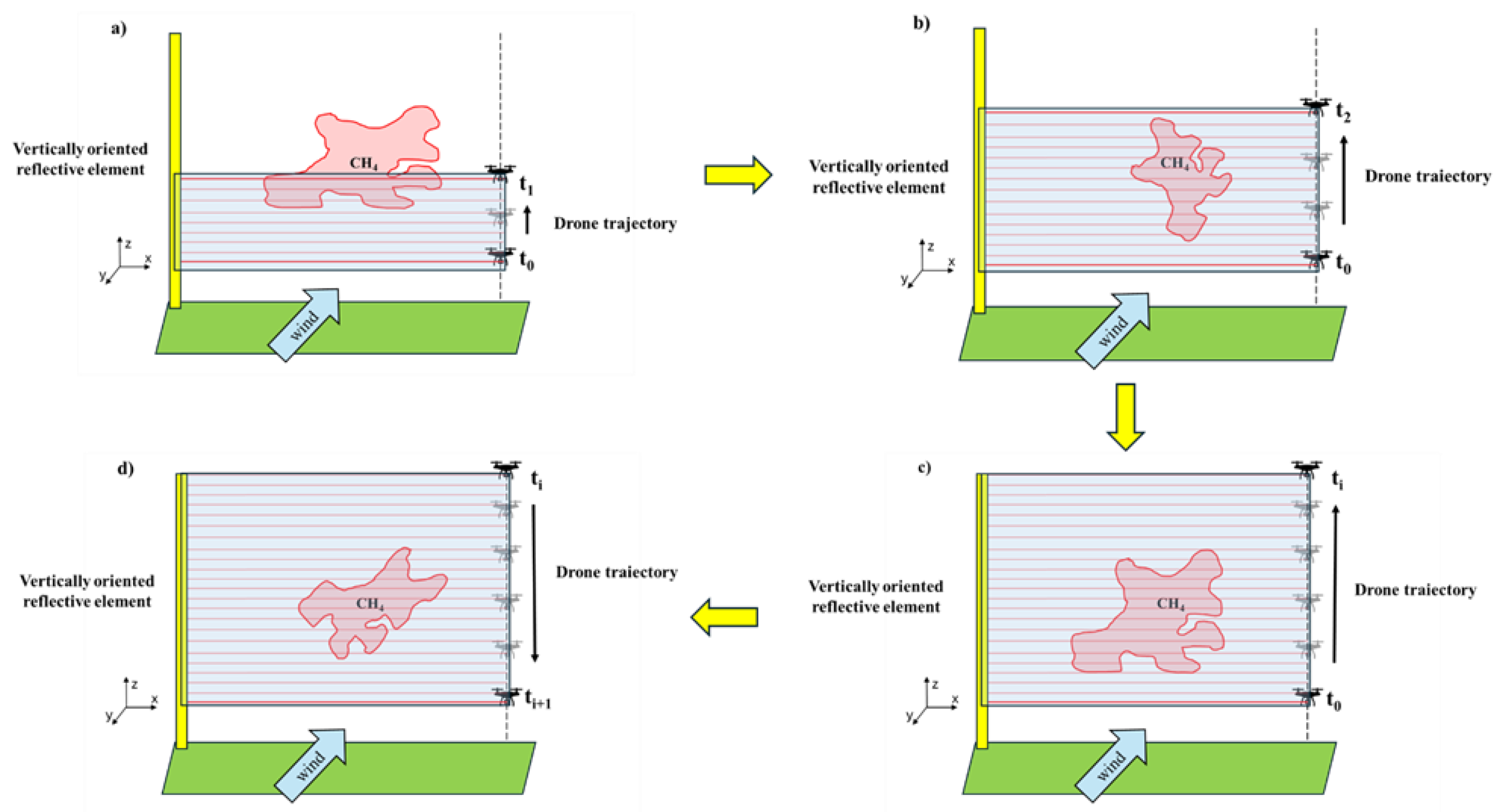
Figure 2.
Distribution of average ppm at 1 m (a), 10 m (b) and 20 m (c) downwind from the source.
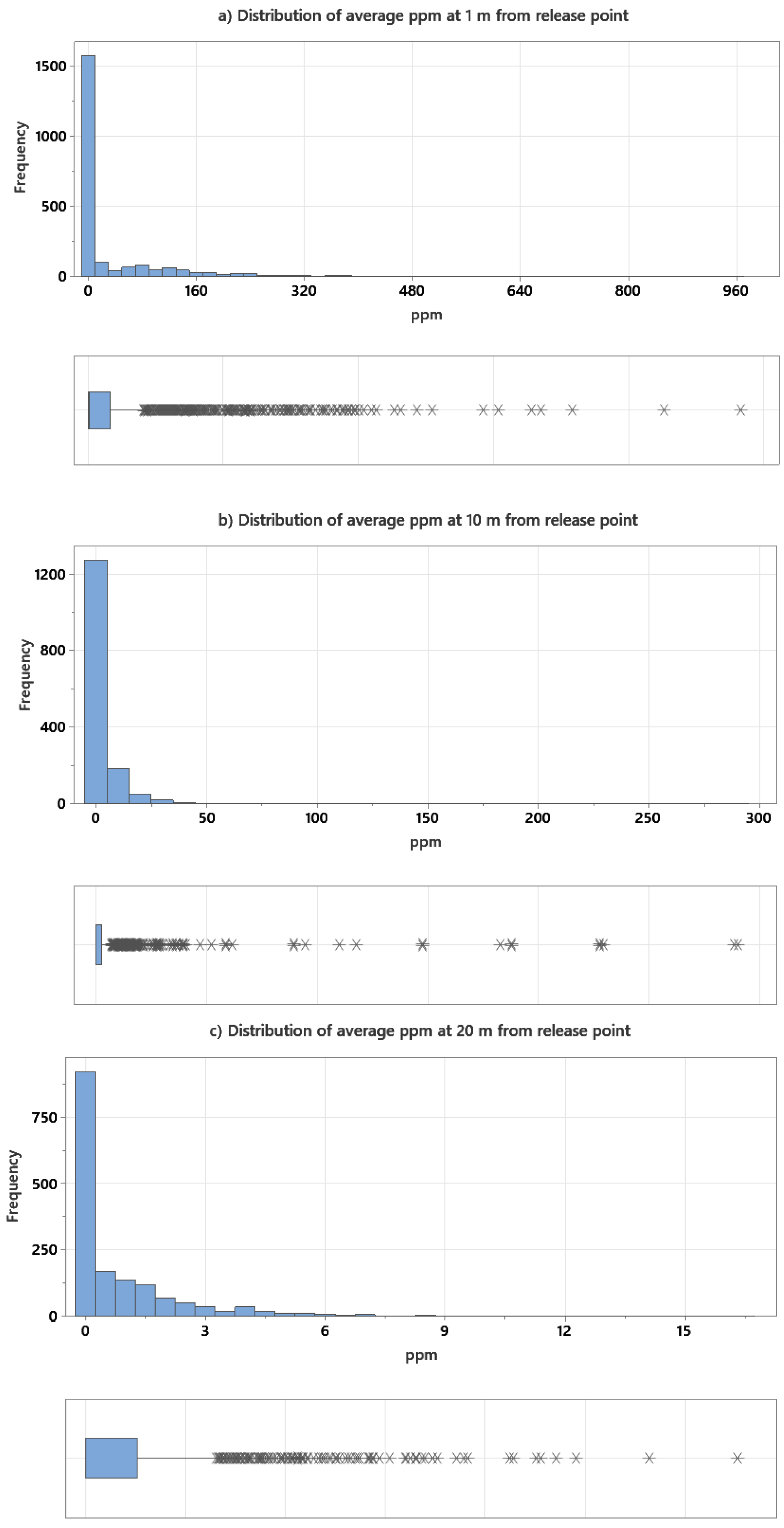
Figure 3.
Emission capture (%) vs distance with Nadiral OP-TDLAS equipped. Simulations carried out under conditions of neutral atmospheric stability (emission rate 0.050 g s-1).
Figure 3.
Emission capture (%) vs distance with Nadiral OP-TDLAS equipped. Simulations carried out under conditions of neutral atmospheric stability (emission rate 0.050 g s-1).
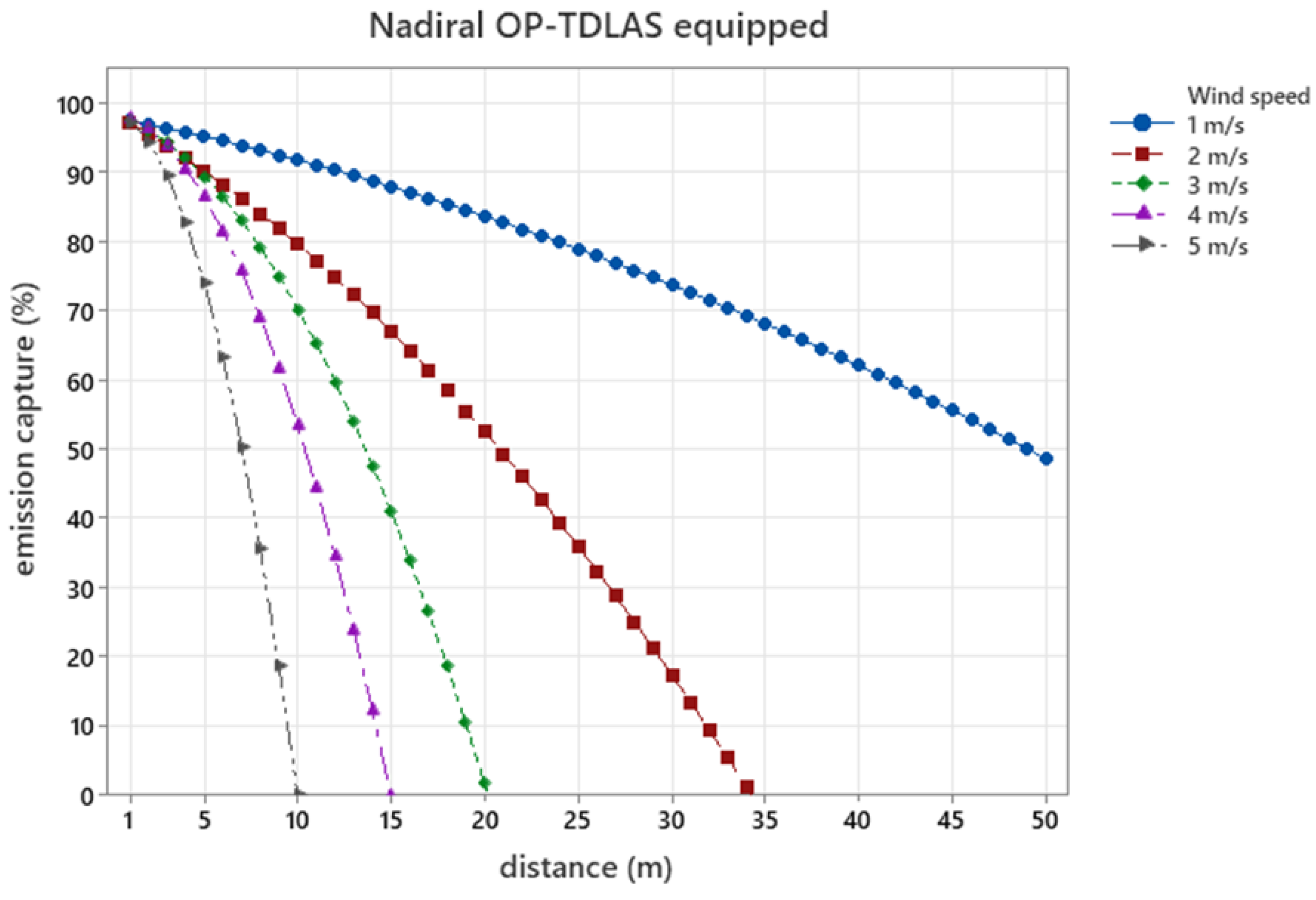
Figure 4.
Emission capture (%) vs distance with Horizontal OP-TDLAS equipped. Simulations carried out under conditions of neutral atmospheric stability (emission rate 0.050 g s-1).
Figure 4.
Emission capture (%) vs distance with Horizontal OP-TDLAS equipped. Simulations carried out under conditions of neutral atmospheric stability (emission rate 0.050 g s-1).
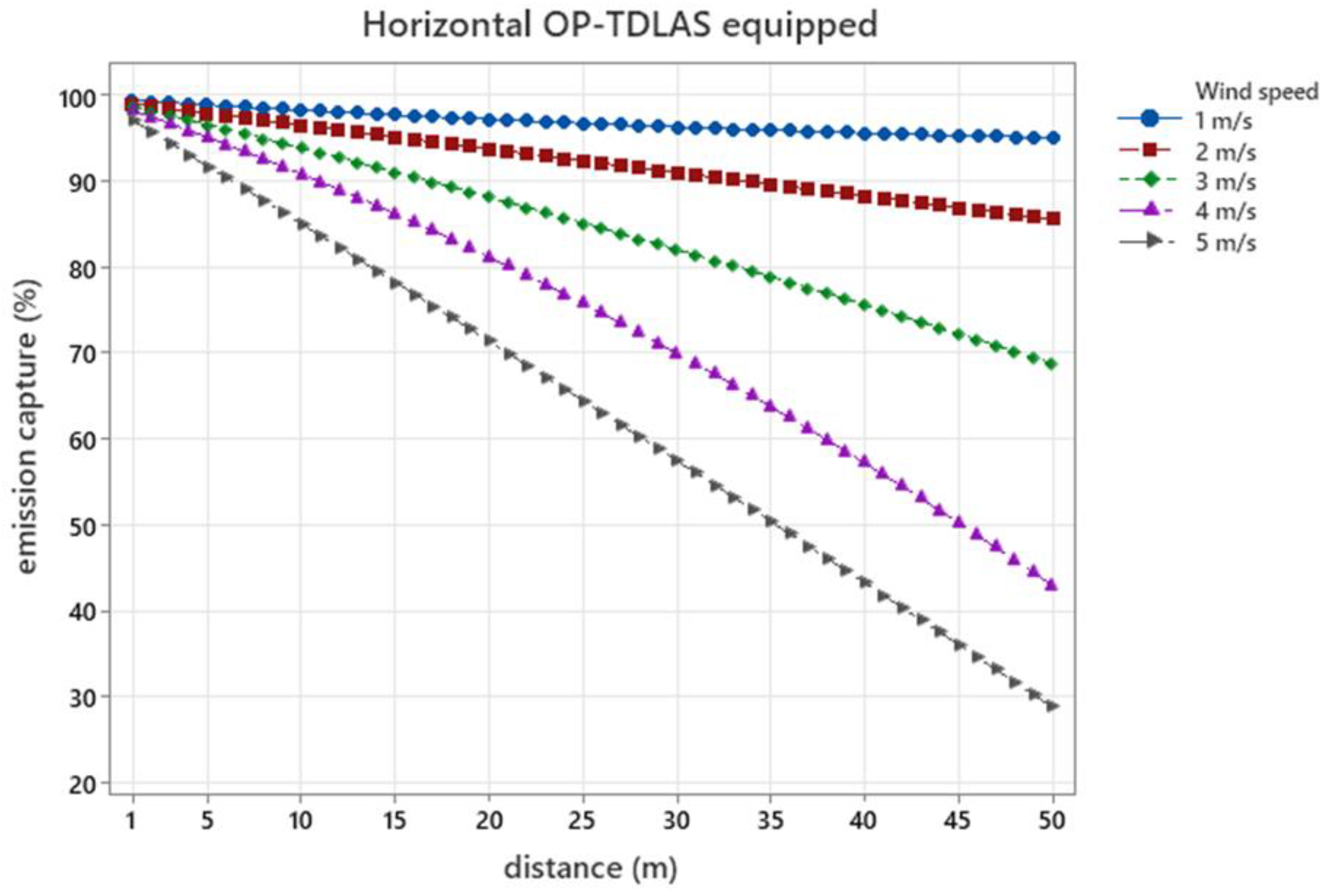
Figure 5.
Vertical Profile Concentration at 1 m, 10 m and 20 m downwind from the source.
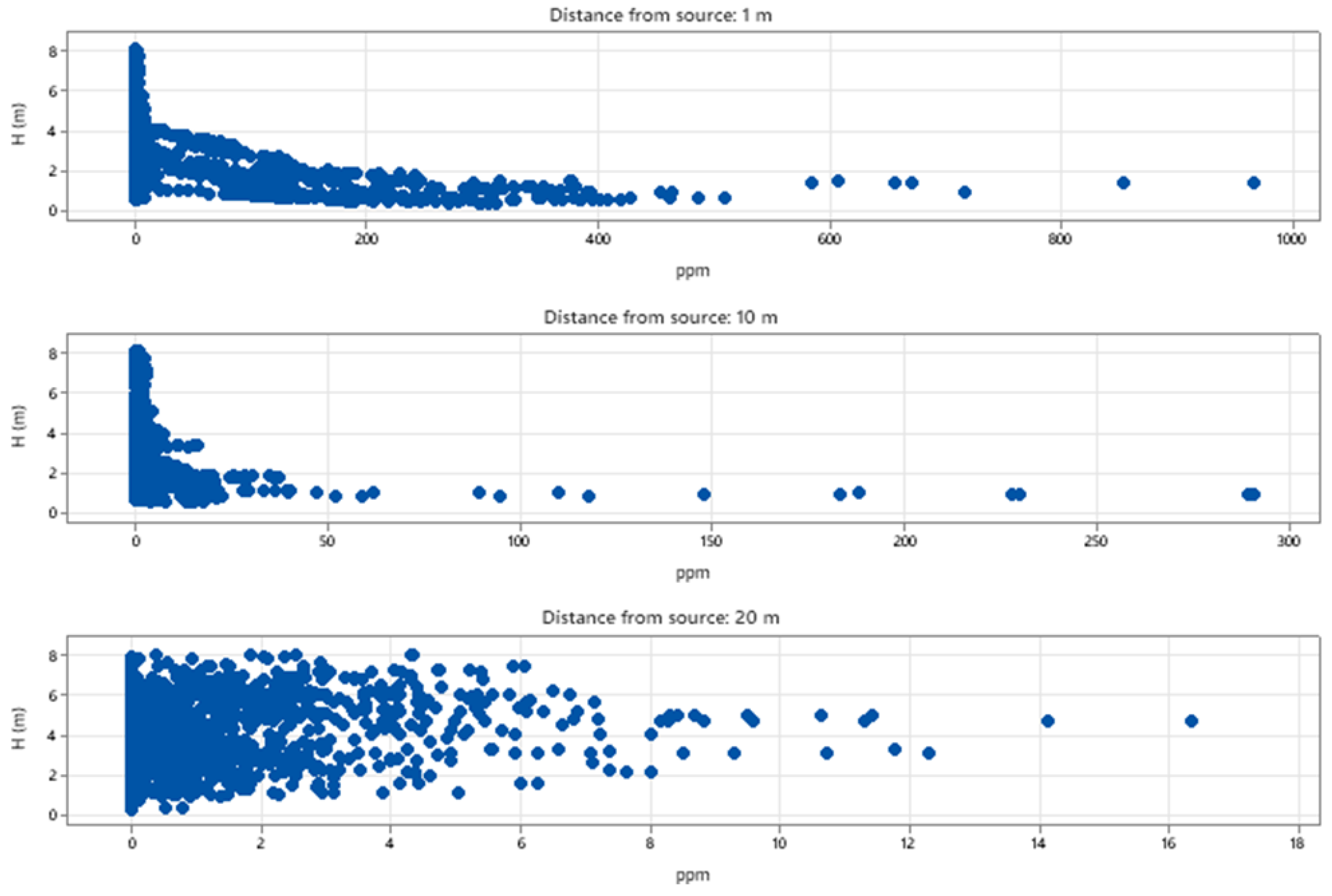
Figure 6.
Recovery rates for scalar and logarithmic wind approach.
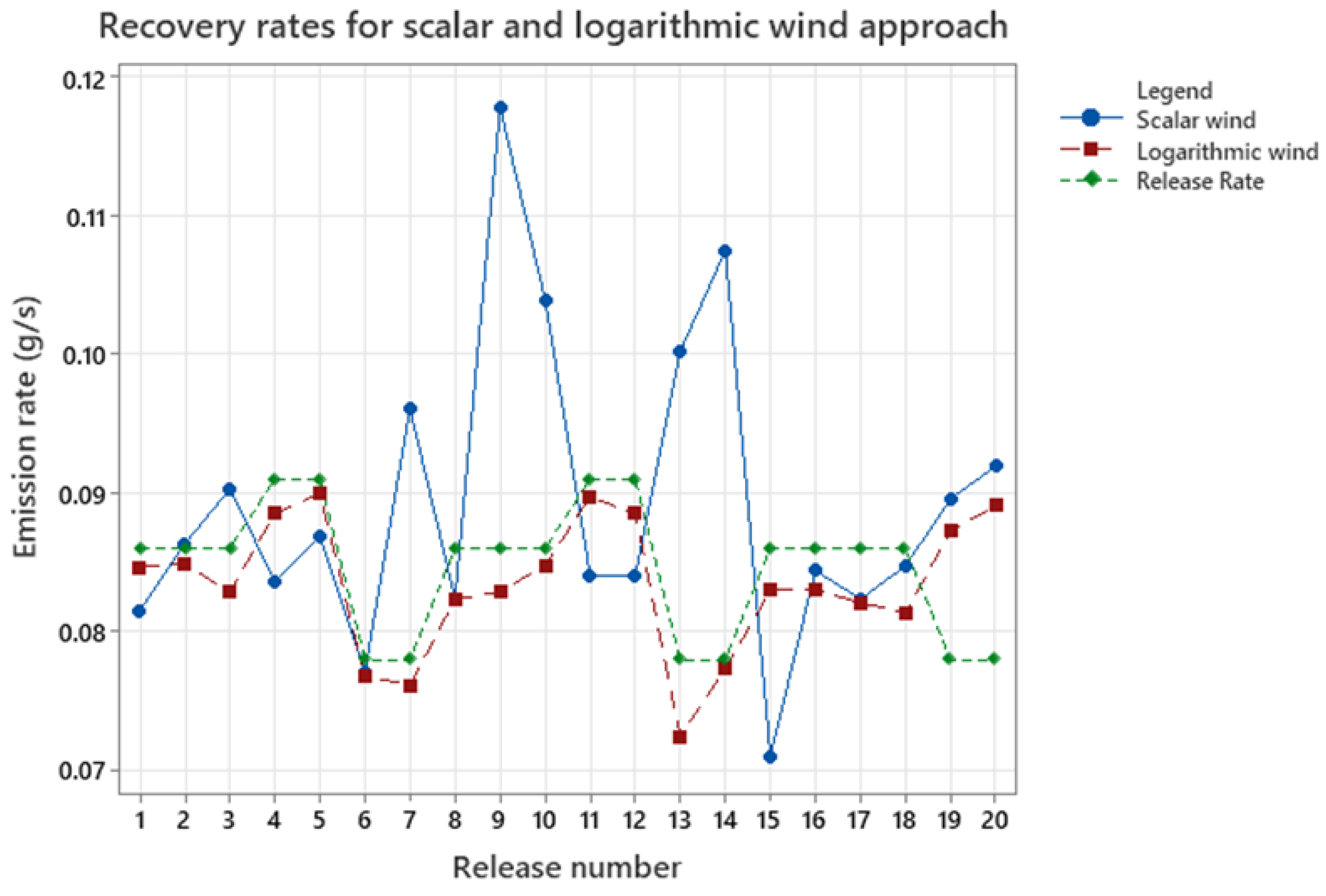
Figure 7.
Interval plot of LW and SW approach for different distance from source.
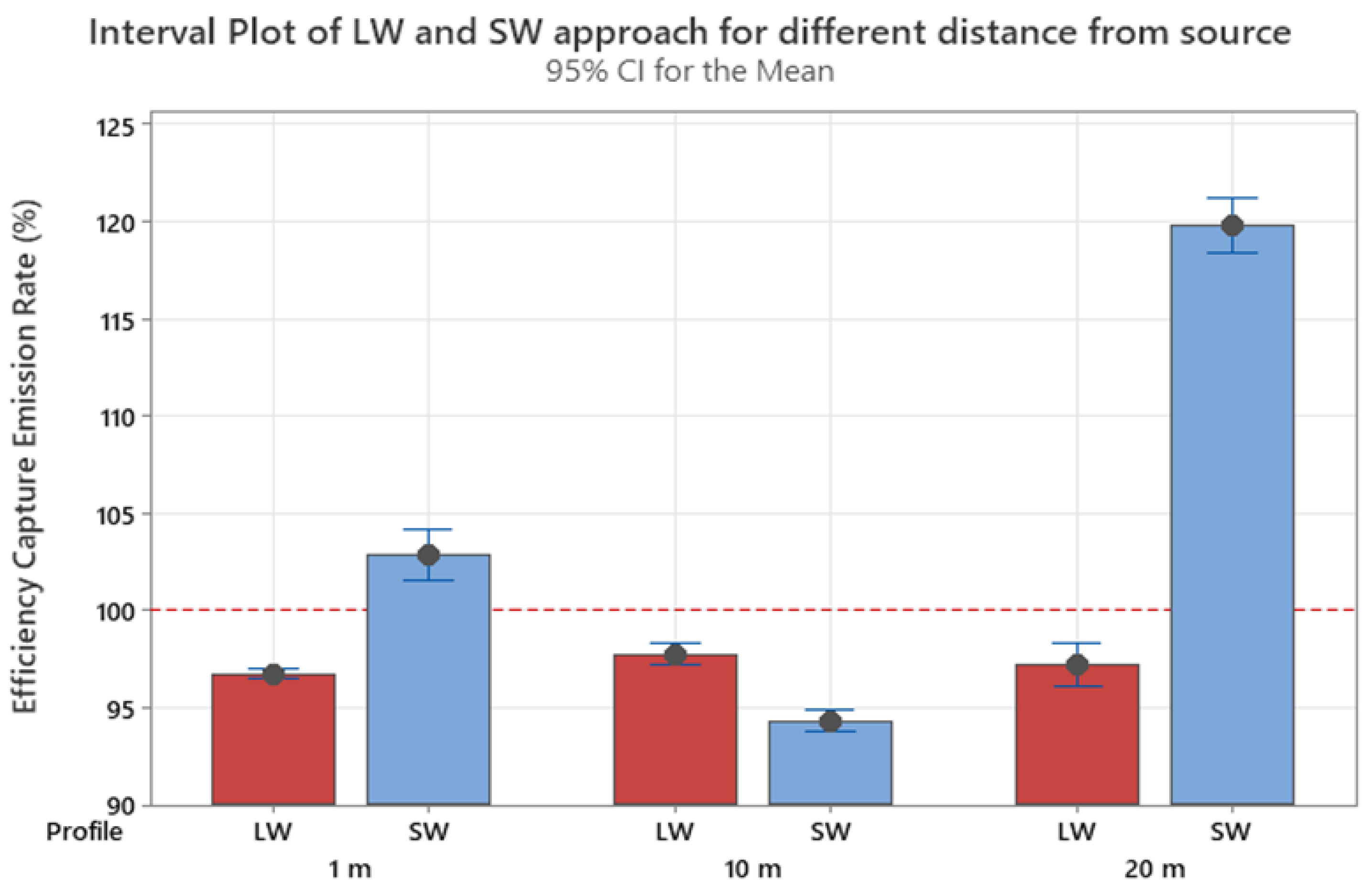
Figure 8.
Contour plot of Mean error (%) vs distance vs wind speed for LW approach.
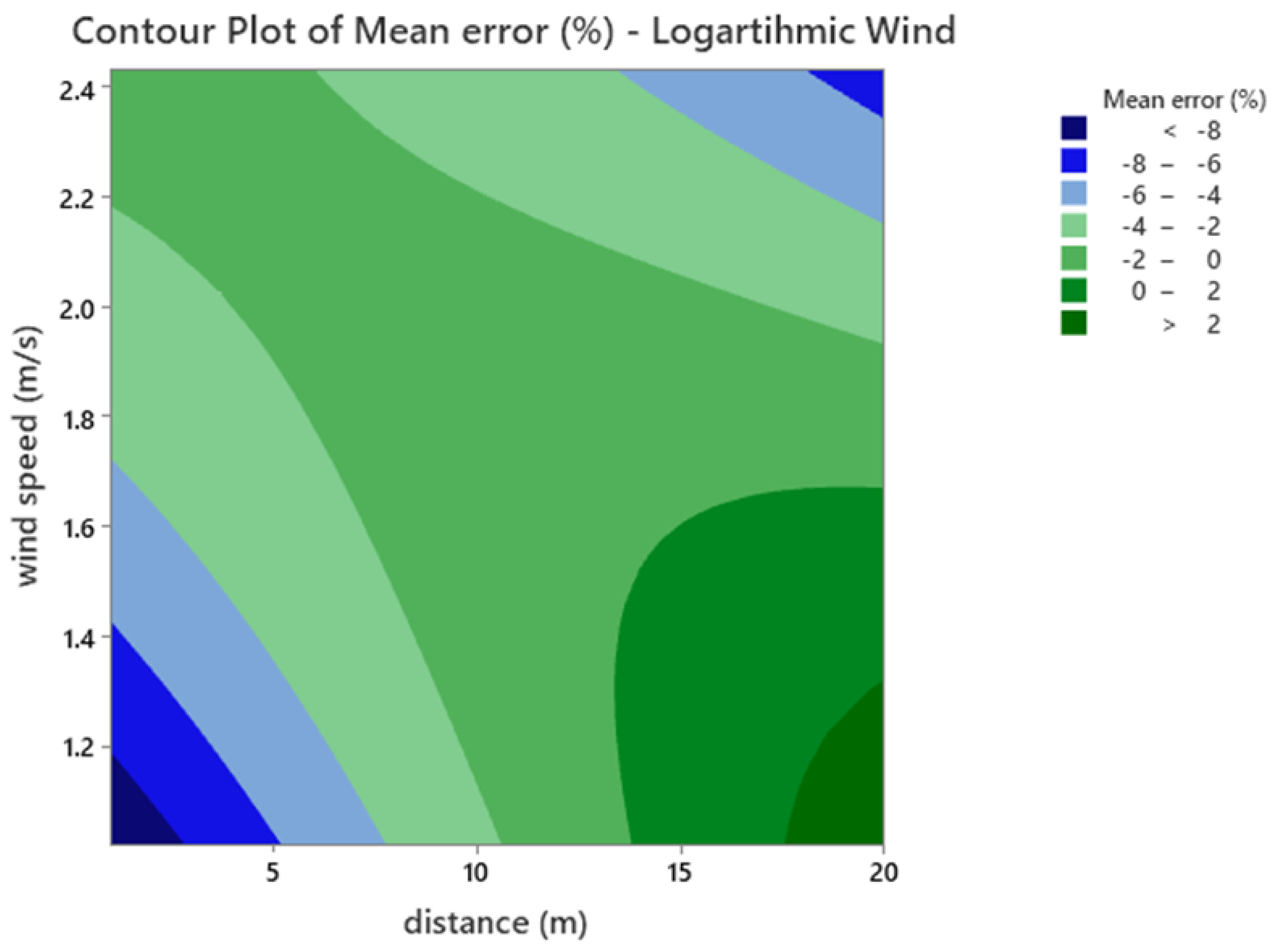
Figure 9.
Contour plot of Mean error (%) vs distance vs wind speed for SW approach.
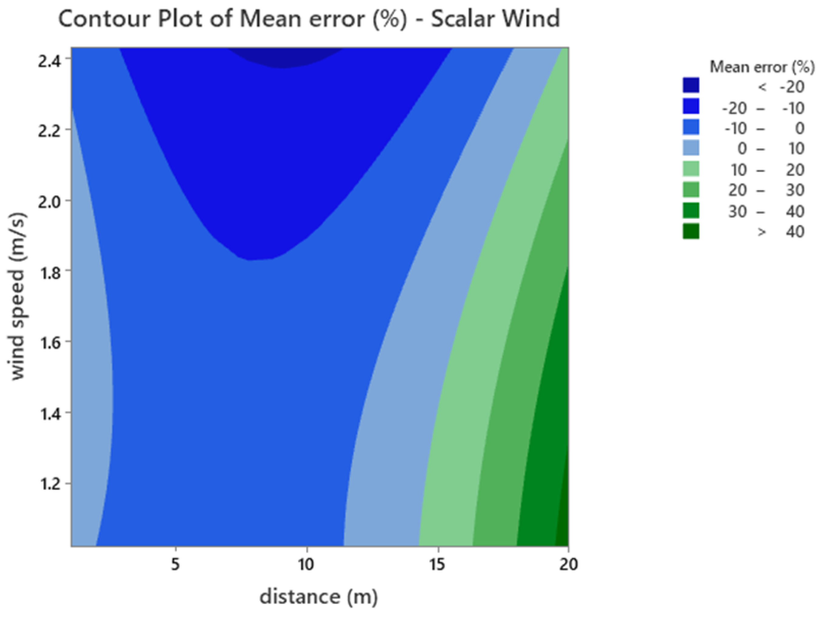

Table 1.
Summaries of controlled release test.
| Date | Number test | Time (Take off – Landing) |
Downwind distance [m] |
Release Rate [g s-1] |
Mean Wind speed [m s-1] |
Mean Wind direction [deg Nord] |
Angle between wind and plane [deg Nord] |
|---|---|---|---|---|---|---|---|
| 15/01/2024 | 1 | 11:28:05 - 11:28:54 | 1 | 0.086 ± 0.006 | 2.32 ± 0.34 | 266 ± 20 | 82 ± 20 |
| 2 | 11:35:03 - 11:35:52 | 1 | 0.086 ± 0.007 | 2.41 ± 0.30 | 294 ± 28 | 84 ± 28 | |
| 3 | 11:42:22 - 11:43:12 | 1 | 0.086 ± 0.009 | 2.02 ± 0.32 | 313 ± 18 | 84 ± 18 | |
| 4 | 12:00:05 - 12:00:52 | 10 | 0.091 ± 0.009 | 1.33 ± 0.15 | 311 ± 16 | 87 ± 16 | |
| 5 | 12:06:26 - 12:07:07 | 10 | 0.091 ± 0.008 | 1.77 ± 0.25 | 288 ± 25 | 96 ± 25 | |
| 6 | 12:20:03 - 12:20:54 | 20 | 0.078 ± 0.007 | 2.42 ± 0.62 | 302 ± 20 | 98 ± 20 | |
| 7 | 12:26:01 - 12:26:51 | 20 | 0.078 ± 0.006 | 2.43 ± 0.77 | 299 ± 26 | 101 ± 30 | |
| 16/01/2024 | 8 | 15:24:16 - 15:25:01 | 1 | 0.086 ± 0.007 | 1.64 ± 0.30 | 302 ± 27 | 81 ± 27 |
| 9 | 15:31:01 - 15:31:53 | 1 | 0.086 ± 0.009 | 1.97 ± 0.51 | 288 ± 31 | 101 ± 25 | |
| 10 | 15:39:12 - 15:40:00 | 1 | 0.086 ± 0.007 | 1.33 ± 0.18 | 143 ± 21 | 104 ± 21 | |
| 11 | 15:47:01 - 15:47:52 | 10 | 0.091 ± 0.008 | 1.28 ± 0.08 | 283 ± 18 | 86 ± 21 | |
| 12 | 15:52:25 - 15:53:04 | 10 | 0.091 ± 0.007 | 1.49 ± 0.21 | 247 ± 15 | 92 ± 23 | |
| 13 | 15:57:12 - 15:58:01 | 20 | 0.078 ± 0.007 | 1.96 ± 0.27 | 304 ± 25 | 91 ± 25 | |
| 14 | 16:05:42 - 16:06:33 | 20 | 0.078 ± 0.007 | 1.46 ± 0.25 | 259 ± 23 | 103 ± 42 | |
| 17/01/2024 | 15 | 10:19:18 - 10:20:02 | 1 | 0.086 ± 0.008 | 1.91 ± 0.11 | 96 ± 18 | 88 ± 18 |
| 16 | 10:30:02 - 10:30:52 | 1 | 0.086 ± 0.008 | 1.77 ± 0.07 | 64 ± 12 | 85 ± 12 | |
| 17 | 10:35:27 - 10:36:03 | 1 | 0.086 ± 0.006 | 1.93 ± 0.05 | 92 ± 16 | 102 ± 16 | |
| 18 | 10:45:01 - 10:45:47 | 1 | 0.086 ± 0.009 | 1.02 ± 0.08 | 69 ± 21 | 82 ± 19 | |
| 19 | 11:02:07 - 11:02:56 | 10 | 0.091 ± 0.007 | 0.97 ± 0.10 | 299 ± 23 | 86 ± 23 | |
| 20 | 11:09:03 - 11:09:49 | 10 | 0.091 ± 0.008 | 1.02 ± 0.18 | 280 ± 16 | 86 ± 21 |
Table 2.
Result flux measurement of controlled release test.
| Date | Number test | Downwind distance [m] |
Release Rate [g s-1] |
LW Approach [g s-1] |
SW Approach [g s-1] |
LW | SW |
|---|---|---|---|---|---|---|---|
| Mean Absolute Error |
Mean Absolute Error |
||||||
| 15/01/2024 | 1 | 1 | 0.086 ± 0.006 | 0.085 ± 0.004 | 0.082 ± 0.002 | 3.6% | 5.2% |
| 2 | 1 | 0.086 ± 0.007 | 0.085 ± 0.002 | 0.086 ± 0.003 | 2.1% | 2.3% | |
| 3 | 1 | 0.086 ± 0.009 | 0.083 ± 0.002 | 0.090 ± 0.002 | 3.8% | 5.1% | |
| 4 | 10 | 0.091 ± 0.009 | 0.089 ± 0.006 | 0.084 ± 0.004 | 6.0% | 8.4% | |
| 5 | 10 | 0.091 ± 0.008 | 0.090 ± 0.007 | 0.087 ± 0.004 | 5.5% | 5.3% | |
| 6 | 20 | 0.078 ± 0.007 | 0.077 ± 0.012 | 0.077 ± 0.006 | 6.8% | 5.4% | |
| 7 | 20 | 0.078 ± 0.006 | 0.076 ± 0.010 | 0.096 ± 0.007 | 10.3% | 23.2% | |
| 16/01/2024 | 8 | 1 | 0.086 ± 0.007 | 0.082 ± 0.002 | 0.082 ± 0.003 | 4.5% | 4.6% |
| 9 | 1 | 0.086 ± 0.009 | 0.083 ± 0.002 | 0.118 ± 0.004 | 3.6% | 36.9% | |
| 10 | 1 | 0.086 ± 0.007 | 0.085 ± 0.003 | 0.104 ± 0.003 | 1.9% | 20.8% | |
| 11 | 10 | 0.091 ± 0.008 | 0.090 ± 0.004 | 0.084 ± 0.004 | 3.2% | 8.0% | |
| 12 | 10 | 0.091 ± 0.007 | 0.089 ± 0.007 | 0.084 ± 0.005 | 4.0% | 8.0% | |
| 13 | 20 | 0.078 ± 0.007 | 0.072 ± 0.005 | 0.100 ± 0.006 | 8.9% | 28.4% | |
| 14 | 20 | 0.078 ± 0.007 | 0.077 ± 0.002 | 0.107 ± 0.008 | 5.5% | 37.8% | |
| 17/01/2024 | 15 | 1 | 0.086 ± 0.008 | 0.083 ± 0.002 | 0.071 ± 0.002 | 3.6% | 17.4% |
| 16 | 1 | 0.086 ± 0.008 | 0.083 ± 0.001 | 0.084 ± 0.002 | 3.5% | 2.4% | |
| 17 | 1 | 0.086 ± 0.006 | 0.082 ± 0.002 | 0.082 ± 0.003 | 4.5% | 4.4% | |
| 18 | 1 | 0.086 ± 0.009 | 0.081 ± 0.003 | 0.085 ± 0.004 | 5.4% | 3.8% | |
| 19 | 10 | 0.091 ± 0.007 | 0.087 ± 0.005 | 0.090 ± 0.006 | 5.8% | 5.8% | |
| 20 | 10 | 0.091 ± 0.008 | 0.089 ± 0.004 | 0.092 ± 0.008 | 4.1% | 6.7% |
Disclaimer/Publisher’s Note: The statements, opinions and data contained in all publications are solely those of the individual author(s) and contributor(s) and not of MDPI and/or the editor(s). MDPI and/or the editor(s) disclaim responsibility for any injury to people or property resulting from any ideas, methods, instructions or products referred to in the content. |
© 2025 by the authors. Licensee MDPI, Basel, Switzerland. This article is an open access article distributed under the terms and conditions of the Creative Commons Attribution (CC BY) license (http://creativecommons.org/licenses/by/4.0/).
Copyright: This open access article is published under a Creative Commons CC BY 4.0 license, which permit the free download, distribution, and reuse, provided that the author and preprint are cited in any reuse.


