
Submitted:
29 April 2025
Posted:
29 April 2025
You are already at the latest version
Abstract
The effective management of landfills requires advancements in techniques for rapid data collection and analysis of gas emissions. This work aims to refine methane (CH₄) emission data acquired from landfills by applying a robust geostatistical method to drone-collected measurements. Specifically, we use UAV-mounted laser spectrophotometer technology (TDLAS-UAV) to gather rapid, high-resolution data, which can sometimes be noisy due to atmospheric variations and sensor drift. For data handling, the key innovation is the application of the Local Indicator of Spatial Association (LISA) to compute the p-values for observed clusters of observations (or better, of grouped observations). This approach was applied both on an areal basis and on a linear basis, following the order of data acquisition, and it produced comparable results. Very low p-values are considered indicative of non-random clustering, suggesting the influence of an underlying spatial control factor. These results were subsequently validated through independent flux chamber surveys. This validation confirms the reliability and objectivity of our geostatistical method in improving drone-based methane emission assessments. The research highlights the need to optimize drone flight paths to ensure a uniform spatial distribution of data and reduce edge effects. It notes that many CH₄ flux measurements often yield non-detectable results, suggesting a review of detection limits. Future work should refine UAV flight patterns and data processing, with semi-controlled experiments -using known methane sources- to determine optimal acquisition parameters such as flight height, sampling frequency, grid resolution, and wind influence.
Keywords:
methane detection
; UAV acquisition
; Geostatistical analysis
; Flux chamber
; Landfill
1. Introduction
In recent years great attention has been paid to monitoring gas emissions from landfills and detecting leaks in natural gas distribution networks. In landfills, the rate and type of gas production vary over time. Shortly after closure of the landfill (months to years), when gas production is greatest, methane (CH4) is the primary component of the gas, typically accounting for 55% by volume, and carbon dioxide (CO2) accounts for most of the remaining volume (Mønster et al., 2019; European commission, 2000). These components are produced from the anaerobic decomposition of biodegradable organic material. The detection of methane leakage is an environmental issue for the following reasons: i) methane escaping into the atmosphere can lead to potential hazards, including the risk of explosion (Rusín et al., 2022; Berisha and Osmanaj, 2021; Ozcan et al., 2006) and it constitutes an important greenhouse gas; (ii) methane leakage lowers the yield of gas collection and distribution systems and thus represents a wasted source of energy; (iii) the presence of emission points within the landfill may highlight portions of the landfill's impermeable waterproofing cover which are flawed and could constitute preferential pathways for meteoric water infiltration resulting in increased leachate production and the associated costs of disposal and potential groundwater pollution.
Hence, the mitigation of methane emission to atmosphere from landfill gas is targeted as a relevant issue in the European Commission Guidance on landfill gas control (European Commission, 2016).
Gas emission monitoring can be conducted in several ways: soil gas, near surface gases, emission, ambient air, indoor air, (Darynova et. al. 2023, Allen et. al. 2019, Agency for Toxic Substances and Disease Registry, 2024). On the ground, probes can be used to sample soil gas topping the landfill, even at different depths (taking care not to intercept the cover sheet, if present) to determine the soil-pore gas concentration, and then using migration (diffusion) models the flow of gas at the soil-atmosphere interface is inferred (Randazzo et al., 2024). Flux chambers, static or dynamic, allow a direct measurement of flux to be determined (Castro Gámez et al., 2019; Ngwabie et al., 2019; Obersky et al., 2018; Scheutz et al., 2017). In recent years, flux measurement techniques with flux chambers have developed in the direction of a rather rapid response (Jeong et al., 2019; Cassini et al., 2017; Di Trapani et al., 2013).
Other methods of measuring CH4 concentrations at the soil/atmosphere interface, or in the first few meters of the atmosphere, related to possible landfill gas emissions, involve the use of portable analysers based on infrared detectors (IRGA) (Shi et al., 2024; Shah et al., 2019; Martin et al., 2017), absorption spectroscopy (TDLAS) (You et al., 2024; Lando et al., 2016; Zhu et al., 2013), and interferometry (Li et al., 2023; Liu et al., 2018; Dullo et al., 2015). Clearly, the methodological approach, e.g. the areal density of sampling, the gaseous species of interest, and the complementary acquisition of ground-based data largely depends on the purposes of the study. However, due to a pronounced “nugget effect” -often resulting from localized gas exhalation- survey campaigns require a very large number of observations to identify exhalation/emission “hot spots” (Wong C.L.Y., 2018; Pratt et al., 2013; Scheutz et al., 2011).
In order to reduce both the time and cost of acquisition campaigns—and to enable data collection in inaccessible areas—UAV-mounted sensors offer significant improvements in acquisition speed and study area coverage (Fosco et al., 2024; Yong et al., 2024; Abichou et al., 2023). After data collection, the processing phase becomes critical. Depending on the measurement method, it may be necessary to filter out noise (such as false positives) before identifying points or areas with fluxes or concentrations that exceed the local background (Barchyn et al., 2019; Barchyn et al., 2017; Emran et al., 2017). Typically, detecting these “hot spots” requires geostatistical techniques. This can involve building a two-dimensional model of the spatial distribution through interpolation techniques (e.g., Morales et al., 2022; Allen et al., 2019; Mackie & Cooper, 2009) or applying the Local Indicator of Spatial Association (LISA) analysis (e.g., Anselin, 1995; Anselin and Xun, 2019).
This work aims to verify whether drone surveys can effectively identify gaseous emissions from both capped and uncapped landfill sectors. Accurate identification requires proper data handling to overcome uncertainties inherent in ambient air measurements -taken over an air column of about 10 m- which are affected by factors such as background variability, wind speed, and instrumental error.
The UAV-mounted TDLAS sensor generates a vast number of observations, resulting in a distribution of values that can be challenging to interpret. Therefore, this study focuses on advanced statistical processing of the data to identify significant clusters of high CH₄ values that are unlikely to occur by chance.
To assess the performance of the UAV-based surveys and our statistical approach, the results were compared with landfill gas flow measurements obtained via flux chambers at the soil-atmosphere interface. Although these flux chamber measurements carry their own uncertainties, they provide gas flux values that are less influenced by air column averaging and wind effects.
2. Materials and Methods
2.1. Equipment
Sensor for CH4 UAV Monitoring
A sensor based on Tuneable Diode Laser Absorption Spectroscopy (TDLAS), also known as a laser spectrophotometer, was used to measure methane (CH4) concentrations. This sensor utilizes a laser source that emits a precisely tuned beam at a specific frequency. This frequency is chosen to be readily absorbed by methane gas molecules, while minimizing interference from other airborne compounds. The sensor then detects the returning laser beam with a receiving device.
The instrument has several ports for connection and communication with other systems (a micro USB port that provides power supply, a standard USB port that enables bi-directional data transfer with a data logger and the drone itself, a microSD card slot for storing hardware upgrade files). For easy integration onto the drone, the equipment features pre-drilled holes in its casing. Lightweight yet robust, custom-moulded brackets are securely fastened to these holes using mechanical systems.
The sensor system also includes a data logger that has the role of acquiring information from the TDLAS, RTK (real time kinematic) system, and altimeter, coupling methane measurement with the coordinates and height data.
The data-logger also exchanges important information to and from the UAV system, such as flight telemetry, loading of preset routes for automatic mode flight activities and sensor control.
With the TDLAS technology, the CH4 concentration (ppm*m) is determined over the distance between the sensor and the ground, i.e. the height above the ground. Therefore, it is necessary for the system to accurately scan and keep constant the flight elevation, as so far as possible, to make observations comparable. The UAV system is equipped with its own autonomous height assessment system to avoid relying on pre-loaded maps (which were found to be prone to significant errors). This part of the system consists of an additional radar altimeter that measures directly the UAV - ground distance and allows the UAV to fly in a “Terrain Following” mode. Thus, even when flying over jagged planes, the distance between the ground plane and the UAV always remains constant.
UAV platform
The TDLAS sensor was mounted on a quadricopter with a mass of 4 kg and a maximum takeoff weight of 6.14 kg. The quadricopter system represented the best choice for reliability, in-flight stability, payload portability and maximization of flight time. The chosen system was then equipped with the above mentioned RTK system which provides excellent precision for georeferencing. The power system, consisting of two batteries operating simultaneously, ensured flight times of about 30 minutes, taking into account the increased power consumption due to the presence of the sensor and the data-logger. Additional plus value inherent in four-motor systems is in-flight manoeuvrability and precision of movement both when used with manual flight and when operated by automatic flight. Table 4 summarises the UAC system specs.
Flux chamber and flux determination
Landfill gas emissions were estimated following the procedure illustrated in Appendix B of SNPA (2018). As provided for in the guideline, flow measurements were conducted using a static non-stationary measurement system1 consisting of a handheld chamber connected to the sensors box. In particular, the capacity of the chamber is 11.2 liter and it is made of steel and Teflon. Inside the chamber, a mixing device and sensors for pressure, humidity, and temperature are installed. Finally, its circular base area is 6.697E-02 m2. The system is equipped with the following sensors:
- PID (Photo Ionization Detector): for measuring Volatile Organic Compounds (VOC) with a 10 eV PID lamp. Sensitive to a wide range of organic substances (and some inorganic substances such as NH3, H2S); the reading is given as isobutylene equivalent, (Accuracy < 3% of the reading).
- IR (Non-Dispersive Infrared Absorption, NDIR): for measuring CO2, (Accuracy < 3% of the reading).
- IR-TLDAS (Infrared Spectroscopy with Tunable Laser Diode Spectrometer): combined with a multipass cell for measuring CH4, (Accuracy < 3% of the reading).
- Ec (Electrochemical cell): for measuring H2S, (Accuracy < 3% of the reading).

Table 5.
Gas concentration ranges measurable by the sensors.
| Sensor | Target | Measurable range | Resolution (ppm) |
|---|---|---|---|
| TD LAS | CH4 | 0.1 ppm – 10% vol | 0.1 |
| IR | CO2 | 0-4000 ppm | 1 |
| PID | VOCs | 0-50 ppm | 1 |
| EC | H2S | 0-100 ppm | 1 |
At each measurement point, data acquisition for flux calculation required approximately 3 to 5 minutes, that is the time span in which a linear increase of gas concentrations is generally observed. Curves of real-time concentration C(t) versus time were generated graphically by the bundled software, which is installed in the handheld computer, and the relative slope gradient for each compound was calculated. The equation that describes the interpolation curve is:
where:
C(t)=αt+β
β is the y-intercept, corresponding to the expected value of C when t=0.
α is the slope of the regression line, i.e. the increasing rate of C with time (dC/dt).
Dimensions of the flux chamber barometric pressure data, air temperature and the slope gradient of the curve (α ppm/sec), were used for deriving the flux values in moles per square meter per day (mol∙m-2 ∙d−1) as defined by the equation (Virgili et al. 2008):
Flux=α Ack
The Ack factor is related to the physical properties of the flux chamber and the environmental sampling parameters (SNPA, 2018).
where:
- 86.400 is the number of seconds in a day [sec d−1];
- 106 is the conversion factor from ppm (in α) to mol∙mol−1;
- Patm is the atmospheric pressure [Pa];
- Vc is the net volume of the chamber [m3];
- R = 8.314472 is the universal gas constant [ m3∙Pa∙K−1∙mol−1];
- T is the air temperature [°K];
- AC is the base area of the chamber [m2].
Weather data monitoring
Environmental conditions, including soil and atmospheric parameters, can greatly affect CH4 emission from soil (e.g. Wu et al., 2023) as well as the CH4 detection along the air-column (e.g. He et al., 2021; Yang et al., 2022). Weather monitoring at the site was carried out during the survey and in the four days preceding it. This was necessary to contextualize the emission phenomena based on any meteorological phenomena that may have occurred. Monitoring in the days prior aimed to verify the absence of rainfall and/or meteorological events of an unusual magnitude for the period of the year and for the area of interest, thereby excluding the possibility of anomalous emission profiles induced by such events. Weather data were acquired by a weather station, mounted on tripods; technical specification as well as data acquired during the survey are provided in the supplementary material.
2.2. Sampling Strategies
Data collection was carried out in four areas as illustrated in Figure 1.
Areas A1 and A2 are two small plots located outside the main landfill body. Currently used for agricultural purposes (specifically, for growing animal fodder), they serve as local reference sites for soil emissivity studies. A drone flight over Area A1 yielded 469 methane (CH4) observations. Area A2, situated approximately 300 meters south of Area A1, underwent two flux measurements using a flux chamber for CH4 and CO2.
Area B, approximately 60×20 m large, is located on a steep slope of the landfill where waste is still being disposed, and where a final cover (capping) has not yet been applied. In Area B, drone surveys yielded 658 CH4 measurements, and six points were measured for CH₄ and CO₂ flux using a flux chamber.
Area C is the main study area, with a surface of approximately 3 ha. Following the completion of landfill operations in 2021, a specialized plastic sheet, a high-density polyethylene (HDPE) geomembrane, was installed as a final cover (capping). A system of biogas wells and an active suction system are used in this area to collect the biogas and convert it into energy. The biogas wells are regularly inspected and cleaned to ensure they are working properly. A stabilized, unpaved track runs circularly throughout the site. Most of the biogas suction system is underground except for some above-ground lines. Within the site, there are three collectors for the biogas capture lines, two located in the central area of the lot and the third positioned at the foot of the slope. Drone surveys in Area C yielded 2552 methane (CH4) measurements, and flux measurements (CH4 and CO2) were conducted at 37 points. In all areas the acquisition parameters, including flight elevation (10 m agl) were the same. The data acquisition pattern is reported in Table 5.
3. Results
Data were acquired in the four areas illustrated in Figure 1: A1, A2, B and C (where areas A1 and A2, are representative of the background scenario outside the landfill) with different expected emission characteristics.
The drone and flow chamber measurements were recorded via methods that do not return completely comparable results. Specifically, the CH4 observations acquired from the drone-mounted sensor returns a concentration, expressed in ppmv*m, representing the CH4 concentration along the column of air (traversed by the TDLAS laser beam) between the ground and the sensor (at a height of approximately 10 m). With the flux chambers, the flux of CO2 and CH4, expressed as moles/m2/d-1, was measured directly at the soil/atmosphere interface.
A non-negligible disturbance component, related to different factors (e.g. (ambient variability of the background, wind speed and instrumental error), is expected for the measurements taken via drone, in the above-mentioned terrain-drone air column, where the escaping gas from surface mixes with atmosphere. On the other hand, acquisition from drone-mounted sensors allows the acquisition of thousands of readings in a very brief time span at extremely low cost. In addition, it is important to highlight that the measurements taken with a flow chamber are point specific and more representative of the actual emission "signal"; however, it is also known that the flux of volatiles is extremely variable in space and time.
Data processing included:
- Descriptive statistics of raw data obtained from the drone sensor (CH4) and from flow chamber (CH4 and CO2) for each investigated area and the comparison between the dataset of each surveyed area
- Spatial distribution of raw data
- Organization of CH4 drone-derived data according to the following steps:
- Grouping of raw observations
- Definition of the statistical indicator to assign to the grouped observations.
- Definition of the threshold value (TV).
- Contiguity analysis of grouped observations exceeding the TV (clustering).
- Calculation of the probabilities that the clustering is random.
- Comparison between non-random clustering and measurements from the flow chamber
The following paragraphs describe in detail the results of the data processing.
3.1. Descriptive Statistics of Raw Data
Table 6 presents the descriptive statistics for drone and flux chamber measurements collected within the studied areas. As highlighted in Figure 2 (left and right), the distributions of CH4 (ppm*m) values in areas B and C largely fit, i.e. no significant difference in CH4 values is observed between capped and uncapped sections within the landfill. Instead, the background area (A1) located outside the landfill exhibits significantly lower values, particularly at higher percentiles. Specifically, CH4 values in A1 for >90 percentiles are approximately half of those observed in areas B and C.
3.2. Spatial Distribution of Raw Data
The distribution of values acquired by drone and flux chamber is represented in Figure 3 (areas A1 and B) and Figure 4 (area C). To highlight the areas with higher values of drone surveys, the raw observations (ROs) were classified into 3 classes:
- Values below the 25th percentile (P25)
- Values between the 25th and 90th percentiles (P25-P90)
- Values between the 90th and 100th percentiles (P90-max)
In area A1, ROs values greater than P90 identify no spatial structures. No flux measurements were made with the flux chamber in this area.
In area B, several observations exceeding P90 (i.e., values greater than 57 ppm*m) seem to be clustered in small portion of area, approximatively in correspondence with the only two methane flux measurements exceeding the detection limit (Figure 3, bottom). It can be observed that the distance between the flux chamber measurement points and the point with the highest drone-measured values is only a few meters. However, within these few meters, there are also numerous observations with relatively low values; therefore, the relationships between the two types of measurements are not fully clear.
The situation is more complex in area C, the main area of investigation (Figure 4). In the northern and western sectors, the values measured by the drone are relatively low. In other areas of the site, along the measurement acquisition path, the values are extremely variable over very small distances (about a few tens of centimetres). Overall, it is quite difficult to identify spatial structures in the CH4 distribution that can be correlated with the flux measurements. Out of 36 flux measurements, only two showed measurable values, while the rest were below the detection limit (DL).
3.3. Organization and Results of CH4 Drone-Derived Data
Individual raw observations (ROs) collected by the drone show a certain degree of randomness due to sensor errors and, mostly, complex acquisition conditions. To make the data informative and reliable, it is therefore necessary to develop a method of processing the data that highlights the spatial structure of CH4 distribution. The surveying of CH4 spatial structures of emission points/areas is based on two criteria:
- Spatial contiguity: the spatial structure is given by the contiguity of two or more points (or spatial elements) that show values above a certain threshold (binary approach).
- Low probability of randomness: the spatial contiguity of two or more elements, exceeding the threshold, must have a low probability of being random.
Ultimately, the probability of the contiguity of several points (or spatial elements) not being random regulates the identification of the threshold and the number of contiguous elements that define that structure.
These criteria were used to process the data, according to two different approaches: i) a "linear" analysis between observations acquired at successive times and points of the drone's trajectory, and ii) a 2D "spatial" analysis, where raw observations were grouped in areal units (Figure 5).
The "linear" analysis: this method involves grouping ROs (taken in the same spatial and temporal order as detected) into sets of 11 and calculating the P75 for each group. Additionally, the coordinates of the central point within each group (i.e. the coordinates of the 6th observation), are assigned. The original number of n ROs is thus reduced to n/11 (which we will be referred to herein as the "linear grouped observations", LGOs). A threshold value (TV) is set; here the TV is the P90 of the values (P75 of GOs) assigned to the LGOs. The TV splits the grouped observations into 2 sets, i) grouped observations lower that TV (90% of LGOs) and ii) grouped observation higher that TV (i.e. 10% of grouped observations, HLGOs).
According to combinatorial calculation, the probability of randomly obtaining a series x of consecutive (adjacent) HLGOs, given n the total number of LGOs and h the number of HLGOs is given by:
Referring to the data from Area C, it can be seen that the approximately 2550 ROs (see Table 6) are reduced to 232 LGOs (2552/11). Assuming the TV as P90 of the values assigned to all LGOs (i.e the P75 value of the 11 ROs forming a LGO), 22 HLGOs are obtained. In the same area the 22 HLGOs define 2 sets of 4 adjacent HLGOs and 4 sets of 2 adjacent HLGOs. In Figure 6 the adjacent HLGOs are connected by lines to better recognize them.
Next step is to evaluate if these “HLGOs lineaments” may be due to chance. Applying equation [1], the following probability values (p_val%) are obtained (Table 7):
The lower the p_val%, the lower is the probability that the contiguity of x HLGO will occur by chance. Contextually, the higher will be the chance that the contiguity of x HLGO is due to a spatial control factor. In area C, the lowest values of p_val%, (0.0062%) are related to 2 sets of 4 adjacent HLGOs that therefore can rightly be considered correlated with an emissive source of CH4. This conclusion is supported by the flux measurements. In fact, the only two flux measures exceeding the DL (solid red squares, Figure 6) are situated near the linear structures identified by the proposed data processing. The spatial structure formed by only two adjacent HLGOs has a probability of being generated by chance greater than 0.5%. Consequently, there is a lower confidence that these spatial structures could be linked to actual emissive phenomena.
The same procedure was applied to areas A1 and B. Results are showed in Figure 7. In each area only one lineament formed by two adjacent HLGOs was found. These lineaments have the probability of being generated by chance greater than 0.5 (p_val%>0.5), therefore they are considered not fully reliable.
The "2D" spatial analysis: in this case, grouping of ROs was related to a regular hexagonal grid. The hexagonal shape was selected as the most isotropic form. The entire area C was subdivided into 104 hexagons with an apothem of approximately 9 meters. ROs included in each hexagon are grouped into an AGO (areal grouped observation). Unlike LGOs, each AGO consists of a different number of ROs and its graphical representation consists of a hexagon and not a point.
Subsequently, various attributes were assigned to each AGO:
- ID number;
- num_obs: number ROs forming each AGO. Moreover, to ensure the reliability of the statistical attributes assigned to each AGO, a “percentage of coverage” is computed, given by the ratio between number of ROs in the i-AGO and maximum number of ROs in a AGO *100. In Figure 8, the percentage of coverage for each AGO is reported. As can be observed, some AGO consist only of 2 ROs, while others have up to a maximum of 90 ROs.
- main statistics of ROs falling in each single AGO (mean, st_dev, 25p, median, P75, P95, max).
While the CH4 concentration value (ppm*m) assigned to each LGO is given by P75 of the ROs forming that LGO, the value assigned to each AGO is given by the average of the ROs (this is because in some AGOs the number of ROs is very small so it would not appropriate to refer to percentiles).
As in the linear analysis, the HAGOs are referenced as the AGOs exceeding the TV, that is set as the P90 of the values assigned to the AGOs (i.e. HAGOs are the top 10% of all AGOs).
In Figure 9, the outcomes of this processing are shown for area C. Each hexagon was assigned the corresponding value of the AGOs. The TV is set as P90 of all 104 AGOs value. The AGOs exceeding the TV are referred as HAGOs (in red). There are two clusters of HAGOs (n. 123-132-141-142-143 and 126-127-136). HAGOs n. 68, 145 and 164 are excluded from consideration, as they do not represent a cluster (they are not bordered by other HAGOs). The LISA (Local indicator of Spatial Association; Anselin, 2019) approach has been adopted to check if the observed clustering is casual or not. LISA provides a way to analyse spatial autocorrelation at the local level, allowing for the identification of local clusters, spatial outliers, and patterns that might not be apparent when examining the data globally. In particular, when a binary parameter is being investigated, the local joint count (LJC) indicator helps to understand how likely is that the clustering occurred by chance. The evaluation of HAGOs clustering involves the calculation of a pseudo-probability value, pp_val%, which is an estimate based on the number of random permutations rather than being calculated analytically. Therefore, pp_val% is not perfectly comparable to the p_val%, which is analytically calculated for assessing the HLGOs clusters. The higher the number of permutations, the closer the pseudo-probability will be to a theoretical probability. In any case, similar to p_val, the lower pp_val is, the higher the chance that clustering around the ith element is due to a “control factor” governing the spatial distribution of the examined parameter. pp_val% calculations were made using the free and open-source software GeoDa.
Table 8 reports the results of the LJC analysis for area C.
In Figure 10, the hexagons indicating a number of JC not attributable to random circumstances (i.e with pp_val<5%) are highlighted in yellow. Among these, hexagons 142 and 132 (pp_val near 1%) stand out, essentially coinciding with the area where a higher CH4 flux than the DL was measured. For hexagons 127 and 136, located in the southern margin of the investigated area, the pp_val% calculation is possibly affected by the edge effect, as discussed below.
Analogous data processing was conducted for area B (the active filling area, without capping). In this case, since the area is quite small (approximately 60 × 30 m), it was necessary to resize the areal units (hexagons with an apothem of about 2.5 m). A total of 60 hexagons (and therefore 60 AGOs) were obtained. The mean of CH4 values of ROs was assigned to AGO. The clustering of HAGOs is shown in Figure 11. As can be seen in the figure, the only two CH4 flux values above the DL (which are also quite high, at 9.2 and 5.3 mol/m2/g respectively) correspond to, or are in the immediate vicinity (with distances less than 1.5 m) of, the HAGOs. Similar considerations apply to CO2 fluxes (the two highest CO2 values correspond to the points with highest CH4 flux).
Also in Area B, for each HAGO bordered by one or more HAGOs, the probabilities are calculated for the clustering to be a random result. pp_val less than 5% were found in HAGO n. 61 (i.e. clustering around this hexagon was supposed not to be random). The flux measurement inside this hexagon was lower that DL, however another flux measurement 3-4 m from hexagon 61 exceeded the DL.
In the background area A1 (not represented in figure), only three and not clustered HAGOs were found. This result is possibly due to a) a poor data set; b) the limited area investigated and c) the lack of a CH4 emission “structure”. In A1 area no CH4 flux measurements are available.
4. Discussion
4.1. Field Results
CH4 data acquired via UAVs show similar values in areas A1, B, and C in terms of absolute values (Figure 2); however, areas B and C show a higher frequency of potential outliers (i.e., values exceeding the inner fence at 75P + 1.5 IQR) than values in background area A1.
Areas B and C show different characteristics: in Area C (capped), it can be assumed that CH4 production processes are already active (with the maximum CH4 production rate expected within 10 years after capping; IPPC, 2006). In this area, the CH4 signal detected by the drone could be related to: i) fluxes at the soil/atmosphere interface due to capping failures; ii) emissive sources located above the interface (e.g., wells/biogas collection lines). In Area B, which is still in the filling phase, it is possible that the methanogenic anaerobic phase has not yet reached its peak.
The main emission zones detected by UAV generally coincide with the few detectable flux measurements taken with the flux chambers (e.g. area C: hexagons 123, 132, 141, 142, 143 in Figure 9 and Figure 10, and Area B: hexagons 50, 60 ,61 ,73 in Figure 11).
The observed coincidence between non-random HAGOs clusters and locations identified by flux chambers as exhibiting higher CH4 (and CO2) fluxes is undoubtedly encouraging. However, perfect spatial alignment between the two measurement techniques could not be anticipated at a fine scale. This is because the sampling and the analysis principles are different. The TDLAS-on-UAV method produces a weighted average of the CH4 concentration in free air along the vertical drone-ground axis (measured in ppm*m). Differently, with the second approach, the rising over time of the CH4 concentration inside the flux chamber allows the calculation of a mass flux (mol/m2/d). The aforesaid differences between UAV and flux chamber measurements methods can lead to data discrepancies that may be difficult to interpret (Figure 12).
An idealized scenario would involve an undisturbed gas plume rising directly from the emission source to the soil-atmosphere interface (scenario “a” in Figure 12), leading to coincident signals from both acquisition methods. In the real-world scenario, factors like wind (scenario “c” in Figure 12) and/or the lateral displacement caused by the drone's propellers (scenario “b” in Figure 12) can disrupt the plume, resulting in a "misalignment" between measurements taken at the soil-atmosphere interface and those within the overlying air column. Additionally, the presence of above-ground emission sources that generate atmospheric plumes but lack a corresponding flux at the soil-atmosphere interface (scenario “d” in Figure 12) must also be considered.
The measurements carried out with the flux chamber produce data that are more accurate because taken directly on the landfill surfaces. However, they offer discontinuous spatial data coverage that could lead to missing out small emission sources (e.g., a punctual failure of a landfill liner). Instead, TDLAS acquisition on UAV can produce thousands of affordable observations in very short time. In fact, a good flight planning allows an excellent uniform coverage of the survey area. However, these measurements often suffer from the critical acquisition conditions of a UAV (the first 10 m of the air column). In this layer, the original gas flow in the atmosphere undergoes extremely fast and uncontrollable/unpredictable dispersion (dilution) in time and space rapidly occurs.
Hence the need for appropriate statistical techniques to filter the data and verify the existence of spatial structures related to the (higher) values of the observations.
4.2. Methods
The proposed processing of drone data ultimately consists of:
- the identification of spatial structures (i.e. clusters of spatial entities exceeding a threshold value, TV);
- the evaluation that such spatial structures are not randomly distributed (i.e., the probability that they are random is extremely low).
Once a non-random spatial structure is identified, it is compared with the outcome of the flux chambers.
The identification of a non-random spatial structure (linear or areal) includes the following steps:
- 4.
- Grouping of raw observations (ROs)
- 5.
- Defining the statistical indicator to assign to the grouped observations.
- 6.
- Setting the threshold value (TV).
- 7.
- Conducting a contiguity analysis of grouped observations exceeding the TV (clustering).
- 8.
- Calculating the probabilities that the observed clustering is random.
Within each stage of this process, various development options influence the final output. Nevertheless, these stages are interdependent and, to some extent, exhibit self-regulating characteristics. Specifically:
a. Grouping of ROs. The process of spatially aggregating ROs was implemented using two distinct methodologies: linear segmentation and areal unit (hexagonal grid) aggregation. Linear segmentation aggregates ROs acquired sequentially in time and space along the drone's flight path, whereas areal unit aggregation uses hexagons to encompass all drone ROs acquired over a specific area.. These two aggregation methods exhibit contrasting characteristics. Linear aggregation yields linear grouped observations (LGOs) with a uniform number of ROs (11 in this study) and is representative of the drone’s flight direction, translating to consistent statistical reliability. However, this method suffers from incomplete spatial coverage. Conversely, areal unit aggregation yields areal grouped observations (AGOs) that guarantee complete coverage of the survey area. However, the number of ROs within each AGO, and consequently the reliability of the derived statistical parameters, exhibits high variability contingent upon the drone's flight paths. Ideally, each AGO should theoretically encompass a minimum of 20 ROs. In the present study, with 2550 ROs, 104 AGOs were established, resulting in an average of approximately 25 ROs/AGO, nevertheless the numbers of ROs vary between 2 and 90. Moreover, even if the number of ROs within each AGO is adequate, their distribution may still be uneven due to a high concentration of ROs along a preferred pathway, such as the drone’s flight direction. Therefore, it is crucial to emphasize the importance of: i) a UAV flight plan that ensures the most uniform areal coverage possible; ii) considering a reliability index (Figure 8).
b. Selection of statistical indicators to assign to LGOs and AGOs.
Within this study, LGOs were assigned P75 of aggregated ROs, while AGO were assigned the mean of aggregated ROs. Other statistical indicators such as the P50, P75 or P90, etc. could be also assigned. However, the analysis of the available dataset revealed a slight influence of the chosen statistical indicator on the final spatial distribution of HLGOs and HAGOs. For example, see distribution of HAGOs when mean, P50, P75 and max are assigned to AGOs and TV is set at P90 of the chosen statistical indicator (Figure 13).
a. Definition of the threshold value (TV).
Selecting an appropriate Threshold Value (TV) is critical for interpreting the data. A higher TV results in a decrease in the number of HLGOs and HAGOs Consequently, the likelihood of encountering random clusters of two or more adjacent HLGOs and HAGOs diminishes. In essence, increasing the TV reduces the overall number of clusters detected, but strengthens the probability that identified clusters are non-random and attributable to underlying influencing factors (e.g., gas emissions). Conversely, employing a lower TV yields a greater number of HLGOs and HAGOs clusters, but generally, it elevates the probability that these clusters are random occurrences.
b. Contiguity analysis of grouped observations exceeding the TV. This phase is the result of the choices made in the previous phases. The clusters of HLGOs and HAGOS are highlighted (consecutive HLGOs in the case of linear grouping, clustering of hexagons in the case of HAGOs).
c. Calculation of the probabilities that the clustering is random. Following the identification of HLGOs or HAGOs clusters, their statistical significance is evaluated using a p-value and pp-value. This value represents the probability that the clusters are merely random occurrences. For HLGOs clusters, p-value calculation employs combinatorial methods. Although the underlying concept behind p-value calculation is straightforward, computational challenges may arise when dealing with large numbers of LGOs.
Based on the provided shapefile, the open-source software GeoDA is utilized to assess the pp_val of HAGO clusters. Given the total number of AGOs and the number of HAGOs, the software performs 10,000 simulations. In each simulation, HAGOs are randomly distributed across the study area. Subsequently, for each HAGO, GeoDA counts the number of neighbouring HAGOs. For instance, if after 10,000 simulations, an HAGO is found adjacent to other four HAGOs in 23 simulations, the resulting pp_val% would be 23/10,000 × 100 = 0. 23%. At this stage the problem of the "edge effect" may arise. Referring to Figure 13, normally each HAGO borders 6 other elements, HAGOs or AGOs (i.e., hexagons that exceed or do not exceed the TV). When the calculation involves HAGOs at the boundary of the area under investigation, the total number of shared boundaries is less than 6 (e.g. 3 or 4). Therefore, the pp-value calculation could provide lower values (the probability of having one HAGO-HAGO border out of 3 or 4 total edges is lower than if the total number of edges is 6).
As an example, in Figure 10, each n. 126, 127, and 136 HAGOs share 2 bounds with the other HAGOs, but only HAGOs 127 and 136 have pp_val <5%. The edge effect can be a critical issue in data interpretation. For this reason, in planning the field activity, it will be advisable to extend the surveys in a small buffer around the target area. Another factor that influences the values of p_val and pp_val is the selection of TV. As TV decreases, the number of HLGOs and HAGOs increases and consequently the probability of random clustering increases (see Figure 13, plot a and e).
5. Conclusions
The study focuses on the development and validation of a statistical method based on the Local Indicator of Spatial Association (LISA) for processing CH₄ data acquired via UAV. The innovation lies in the systematic grouping of thousands of raw observations to identify spatial structures -clusters of high methane values - that are unlikely to occur by chance. The analysis employs both a linear segmentation approach, which groups sequential observations along the drone’s flight path, and a two-dimensional areal aggregation using a hexagonal grid. In both cases, a threshold value is defined and clusters exceeding this threshold are evaluated for randomness using combinatorial probability and LISA-derived pseudo-probabilities. Flux chamber measurements, which provide precise and localized methane and carbon dioxide flux data at the soil–atmosphere interface, were used as an independent reference to validate the identified statistical patterns. The encouraging correspondence between non-random clusters identified via LISA and the flux chamber data supports the reliability of the proposed method, even though perfect spatial alignment is not expected due to inherent differences in measurement principles.
The study also highlights areas for improvement in both UAV acquisition and flux measurement. In particular, it reveals the importance of an effective data acquisition strategy, including well-planned drone routes, to ensure: i) a uniform areal distribution of observations across the study area; and ii) a buffer zone around the target area to mitigate edge effects. Additionally, CH₄ flow measurements often did not yield detectable methane values, indicating a need to refine the detection limits of the method. Further research should include conducting data acquisition in semi-controlled conditions, where the methane source is known in terms of quantity and location, to determine optimal parameters such as flight height, sampling frequency, grid resolution, and the influence of wind.
Exploring the scalability of this approach to other gases and environmental contexts is also recommended. Despite some limitations, the experimental results from the landfill study are encouraging, demonstrating that the advanced statistical processing of drone data can effectively identify emission hotspots and be reliably validated by independent flux measurements.
Supplementary Materials
The following supporting information can be downloaded at the website of this paper posted on Preprints.org.
| 1 | This type of system is defined as "non-stationary" because, assuming a constant emission flow from the soil, the concentration of analytes in the gas mixture within the chamber increases over time without remaining constant at any point in the chamber. It is termed 'static' because, unlike dynamic chambers where an inert gas flows through the chamber, this system recirculates the gas without any treatment and analyzes it directly in the field. |
References
- Abichou, T.; Bel Hadj Ali, N.; Amankwah, S.; Green, R.; Howarth, E.S. (2023). Using Ground- and Drone-Based Surface Emission Monitoring (SEM) Data to Locate and Infer Landfill Methane Emissions. Methane. Vol. 2, pp. 440-451. [CrossRef]
- Agency for Toxic Substances and Disease Registry (2024) WEB site: Landfill Gas Primer - AnOverview for Environmental Health Professionals. Chapter 4: Monitoring of Landfill Gas https://www.atsdr.cdc.gov/HAC/landfill/html/ch4.html.
- Allen G., Hollingsworth P., Kabbabe K., Pitt J.R., Mead M., Illingworth S., Roberts G., Bourn M., Shallcross D.E., Percival C.J. (2019): The development and trial of an unmanned aerial system for the measurement of methane flux from landfill and greenhouse gas emission hotspots. Waste Management 87 (2019) 883–892. [CrossRef]
- Anselin, L. (1995), Local Indicators of Spatial Association—LISA. Geographical Analysis, 27: 93-115. [CrossRef]
- Anselin L., Xun L. (2019): Operational local join count statistics for cluster detection. Journal of Geographical Systems (2019) 21:189–210. [CrossRef]
- Barchyn, T. E., Hugenholtz, C. H. e Fox,T.A., (2019). Plume detection modeling of a drone-based natural gas leak detection system. Elementa: Science of the Anthropocene. Vol. 7. [CrossRef]
- Barchyn, T., Hugenholtz, C. H., Myshak, S. e Bauer, J., (2017). A UAV-based system for detecting natural gas leaks. Journal of Unmanned Vehicle Systems. [CrossRef]
- Berisha, A. e Osmanaj, L., (2021). Determination of Methane Explosion Level in the Velekince Municipal Solid Waste Landfill. Ecological Engineering & Environmental Technology. Vol. 22 (5), pp. 82–88. [CrossRef]
- Cassini, F., Scheutz, C., Skov, B. H., Mou, Z. e Kjeldsen, P., (2017). Mitigation of methane emissions in a pilot-scale biocover system at the AV Miljø Landfill, Denmark: 1. System design and gas distribution. Waste Management. Vol. 63, pp. 213–225. [CrossRef]
- Castro Gámez, A. F., Rodríguez Maroto, J. M. e Vadillo Pérez, I., (2019). Quantification of methane emissions in a Mediterranean landfill (Southern Spain). A combination of flux chambers and geostatistical methods. Waste Management. Vol. 87, pp. 937–946. [CrossRef]
- Darynova,Z., Blanco,B., Juery,C., Donnat,L. e Duclaux,O., (2023). Data assimilation method for quantifying controlled methane releases using a drone and ground-sensors. Atmospheric Environment: X. 100210. [CrossRef]
- De Molfetta, M. Fosco, D., Renzulli P.A., Notarnicola, B. 2024. Identification and treatment of false methane values produced by the TDLAS technology equipped on UAVs. Integrated Environmental Assessment and Management (2024). Undergoing publication. [CrossRef]
- Di Trapani, D., Di Bella, G., Viviani, G., (2013). Uncontrolled methane emissions from a MSW landfill surface: Influence of landfill features and side slopes. Waste Management. Vol. 33 (10), 2108–2115. [CrossRef]
- Dullo, F. T. Dullo, F. T., Lindecrantz, S., Jágerská, J., Hansen, J. H., Engqvist, M., Solbø, S. A. e Hellesø, O. G., (2015). Sensitive on-chip methane detection with a cryptophane-A cladded Mach-Zehnder interferometer. Optics Express. Vol. 23 (24), 31564. [CrossRef]
- Emran, Bara J., Dwayne D. Tannant, and Homayoun Najjaran. (2017). "Low-Altitude Aerial Methane Concentration Mapping" Remote Sensing 9, no. 8: 823. [CrossRef]
- European Commission, DG Environment (2000): A Study on the Economic Valuation of Environmental Externalities from Landfill Disposal and Incineration of Waste. Final Appendix Report. https://circabc.europa.eu/ui/group/636f928d-2669-41d3-83db-093e90ca93a2/library/809ab9bf-4a37-4ae4-82c0-653115da237b/details.
- European Commission, (2016). http://ec.europa.eu/environment/waste/landfill/pdf/.
- guidance%20on%20landfill%20gas.pdf.
- Fosco, D., De Molfetta, M., Renzulli, P. e Notarnicola, B., (2024). Progress in monitoring methane emissions from landfills using drones: an overview of the last ten years. Science of The Total Environment. Vol. 945, 173981. [CrossRef]
- He, H.; Gao, S.; Hu, J.; Zhang, T.;Wu, T.; Qiu, Z.; Zhang, C.; Sun, Y.; He, S. (2021) . In-Situ Testing of Methane Emissions from Landfills Using Laser Absorption Spectroscopy. Appl. Sci. 2021, 11, 2117. [CrossRef]
- IPCC (Intergovernmental Panel on Climate Change). (2006). 2006 IPCC Guidelines for National Greenhouse Gas Inventories: Waste. Vol. 5, National Greenhouse Gas Inventories Programme.
- Ishigaki, T., Yamada, M., Nagamori, M., Ono, Y., Inoue, Y., (2005). Estimation of methane emission from whole waste landfill site using correlation between flux and ground temperature. Environmental Geology, Vol. 48 No. 7, pp. 845–853. https://ui.adsabs.harvard.edu/link_gateway/2005EnGeo.48..845I/doi:10.1007/s00254-005-0008-0. [CrossRef]
- Jeong, S., Park, J., Kim, Y. M., Park, M. H. e Kim, J. Y., (2019). Innovation of flux chamber network design for surface methane emission from landfills using spatial interpolation models. Science of The Total Environment. Vol. 688, 18–25. [CrossRef]
- Karanjekar, R. V., Bhatt, A., Altouqui, S., Jangikhatoonabad, N., Durai, V., Sattler, M. L., Hossain, M. D. S., & Chen, V. (2015). Estimating methane emissions from landfills based on rainfall, ambient temperature, and waste composition: The CLEEN model. Waste Management, Vol. 46, pp. 389–398. [CrossRef]
- Lando, A. T., Nakayama, H. e Shimaoka, T., (2016). Application of portable gas detector in point and scanning method to estimate spatial distribution of methane emission in landfill. Waste Management. Vol. 59, pp. 255–266. [CrossRef]
- Li, Y., Chen, H., Li, H., Liu, C., Li, J., Chen, Q., Li, K., Zhang, S. e Gu, M., (2023). Ultra-high sensitivity methane gas sensor based on vernier effect in double D-shaped and cryptophane-A film-coated photonic crystal fiber: Design and FEM simulation. Results in Physics. Vol. 52, 106840. [CrossRef]
- Liu, H., Wang, M., Wang, Q., Li, H., Ding, Y. e Zhu, C., (2018). Simultaneous measurement of hydrogen and methane based on PCF-SPR structure with compound film-coated side-holes. Optical Fiber Technology. Vol. 45, pp. 1–7. [CrossRef]
- Mackie, K. R. e Cooper, C. D., (2009). Landfill gas emission prediction using Voronoi diagrams and importance sampling. Environmental Modelling & Software. Vol. 24 (10), 1223–1232. [CrossRef]
- Martin, C. R., Zeng, N., Karion, A., Dickerson, R. R., Ren, X., Turpie, B. N., and Weber, K. J. (2017). Evaluation and environmental correction of ambient CO2 measurements from a low-cost NDIR sensor. Atmos. Meas. Tech., 10, 2383–2395. [CrossRef]
- Morales, R., Ravelid, J., Vinkovic, K., Korbeń, P., Tuzson, B., Emmenegger, L., Chen, H., Schmidt, M., Humbel, S., and Brunner, D., (2022). Controlled-release experiment to investigate uncertainties in UAV-based emission quantification for methane point sources. Atmos. Meas. Tech., 15, 2177–2198. [CrossRef]
- Mønster, J., Kjeldsen, P. e Scheutz, C., (2019). Methodologies for measuring fugitive methane emissions from landfills – A review. Waste Management. Vol. 87, pp. 835–859. [CrossRef]
- Ngwabie, N. M., Wirlen, Y. L., Yinda, G. S. e VanderZaag, A. C., (2019). Quantifying greenhouse gas emissions from municipal solid waste dumpsites in Cameroon. Waste Management. Vol. 87, pp. 947–953. [CrossRef]
- Obersky, L., Rafiee, R., Cabral, A. R., Golding, S. D. e Clarke, W. P., (2018). Methodology to determine the extent of anaerobic digestion, composting and CH4 oxidation in a landfill environment. Waste Management. Vol. 76, pp. 364–373. [CrossRef]
- Ozcan H. K., BORAT M., Sezgin N., Nemlioglu S., Demir G. (2006). Determination of seasonal variations of major landfill gas in Istanbul Kemerburgaz-Odayeri solid waste landfill. Fresenius Environmental bulletin, vol.15, no.4, pp.272-276. https://avesis.iuc.edu.tr/yayin/31e91822-0f70-4955-8c2d-39f3566485db/determination-of-seasonal-variations-of-major-landfill-gas-in-istanbul-kemerburgaz-odayeri-solid-waste-landfill.
- Pratt, C., Walcroft, A. S., Deslippe, J. e Tate, K. R., (2013). CH4/CO2 ratios indicate highly efficient methane oxidation by a pumice landfill cover-soil. Waste Management. Vol. 33 (2), 412–419. [CrossRef]
- Randazzo, A., Venturi, S. e Tassi, F., (2024). Soil processes modify the composition of volatile organic compounds (VOCs) from CO2- and CH4-dominated geogenic and landfill gases: A comprehensive study. Science of The Total Environment. Vol. 923, 171483. [CrossRef]
- Rusín, J., Chamrádová, K., Jastrzembski, T., & Skrínský, J. (2022). Explosion characteristics of a biogas/air mixtures. Chemical Engineering Transactions, 90, 271-276. [CrossRef]
- Scheutz, C., Cassini, F., De Schoenmaeker, J. e Kjeldsen, P., (2017). Mitigation of methane emissions in a pilot-scale biocover system at the AV Miljø Landfill, Denmark: 2. Methane oxidation. Waste Management. Vol. 63, 203–212. [CrossRef]
- Scheutz, C., Fredenslund, A. M., Nedenskov, J., Samuelsson, J. e Kjeldsen, P., (2011). Gas production, composition and emission at a modern disposal site receiving waste with a low-organic content. Waste Management. Vol. 31 (5), 946–955. [CrossRef]
- Shah, A.; Pitt, J.; Kabbabe, K.; Allen, G. (2019). Suitability of a Non-Dispersive Infrared Methane Sensor Package for Flux Quantification Using an Unmanned Aerial Vehicle. Sensors, 19, 4705. [CrossRef]
- Shi, J., Jiang, Y., Duan, Z., Li, J., Yuan, Z. e Tai, H., (2024). Designing an optical gas chamber with stepped structure for non-dispersive infrared methane gas sensor. Sensors and Actuators A: Physical. Vol. 367. 115052. [CrossRef]
- SNPA. Sistema Nazionale per la Protezione dell’Ambiente (2018). Progettazione del monitoraggio di vapori nei siti contaminati. Linea Guida SNPA 15/2018 Appendix B. ISBN: 978-88-448-0922-5. https://www.snpambiente.it/wp-content/uploads/2018/11/Appendice_B_linee_guida_snpa_15_2018.pdf.
- Virgili G., Continanza D., Coppo L. (2008). The FLUX-meter: a portable integrated instrumentation for the measurement of the biogas diffuse degassing from landfills. Giornale di Geologia Applicata 9:73–84.
- Yong, H.; Allen, G.; Mcquilkin, J.; Ricketts, H.; Shaw, J.T., (2024). Lessons learned from a UAV survey and methane emissions calculation at a UK landfill. Waste Management, Volume 180, Pages 47-54. ISSN 0956-053X. [CrossRef]
- You, R., Kang, H., Zhang, X., Zheng, S., Shao, L., Han, J. e Feng, G., (2024). Cubic nonlinear scanning for improved TDLAS-based methane concentration detection. International Journal of Hydrogen Energy.Vol. 86, 14–23. [CrossRef]
- Wong, C. L. Y. (2018). Analysis of the number of flux chamber samples and study area size on the accuracy of emission rate measurements. Journal of the Air & Waste Management Association, 68(10), 1103–1117. [CrossRef]
- Wu, T.; Cheng, J.;Wang, S.; He, H.; Chen, G.; Xu, H.; Wu, S. (2023). Hotspot Detection and Estimation of Methane Emissions from Landfill Final Cover. Atmosphere 2023, 14, 1598. [CrossRef]
- Haoqing Yang, Xiongzhu Bu, Yang Song, Yue Shen (2022): Methane concentration measurement method in rain and fog coexisting weather based on TDLAS, Measurement, Volume 204, 2022, 112091, ISSN 0263-2241. [CrossRef]
- Zhu, H., Letzel, M. O., Reiser, M., Kranert, M., Bächlin, W. e Flassak, T., (2013). A new approach to estimation of methane emission rates from landfills. Waste Management. Vol. 33 (12), 2713–2719. [CrossRef]
Figure 1.
Location of surveyed areas. Areas A1 and A2 are outside the landfill and are taken as background area. Area B is active and not capped; in area C filling is over and the area is provided with capping.
Figure 1.
Location of surveyed areas. Areas A1 and A2 are outside the landfill and are taken as background area. Area B is active and not capped; in area C filling is over and the area is provided with capping.
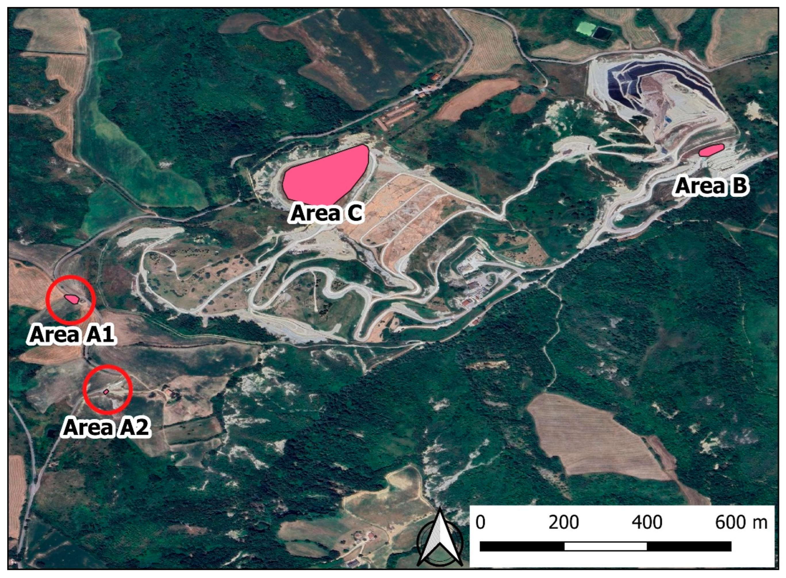
Figure 2.
(left) Distribution of CH4 values, acquired by UAV (ppm*m) in the investigated areas (A1, B, C); (right) Percentiles distribution; arrow marks the difference of distribution of A1 vs. B and C.
Figure 2.
(left) Distribution of CH4 values, acquired by UAV (ppm*m) in the investigated areas (A1, B, C); (right) Percentiles distribution; arrow marks the difference of distribution of A1 vs. B and C.
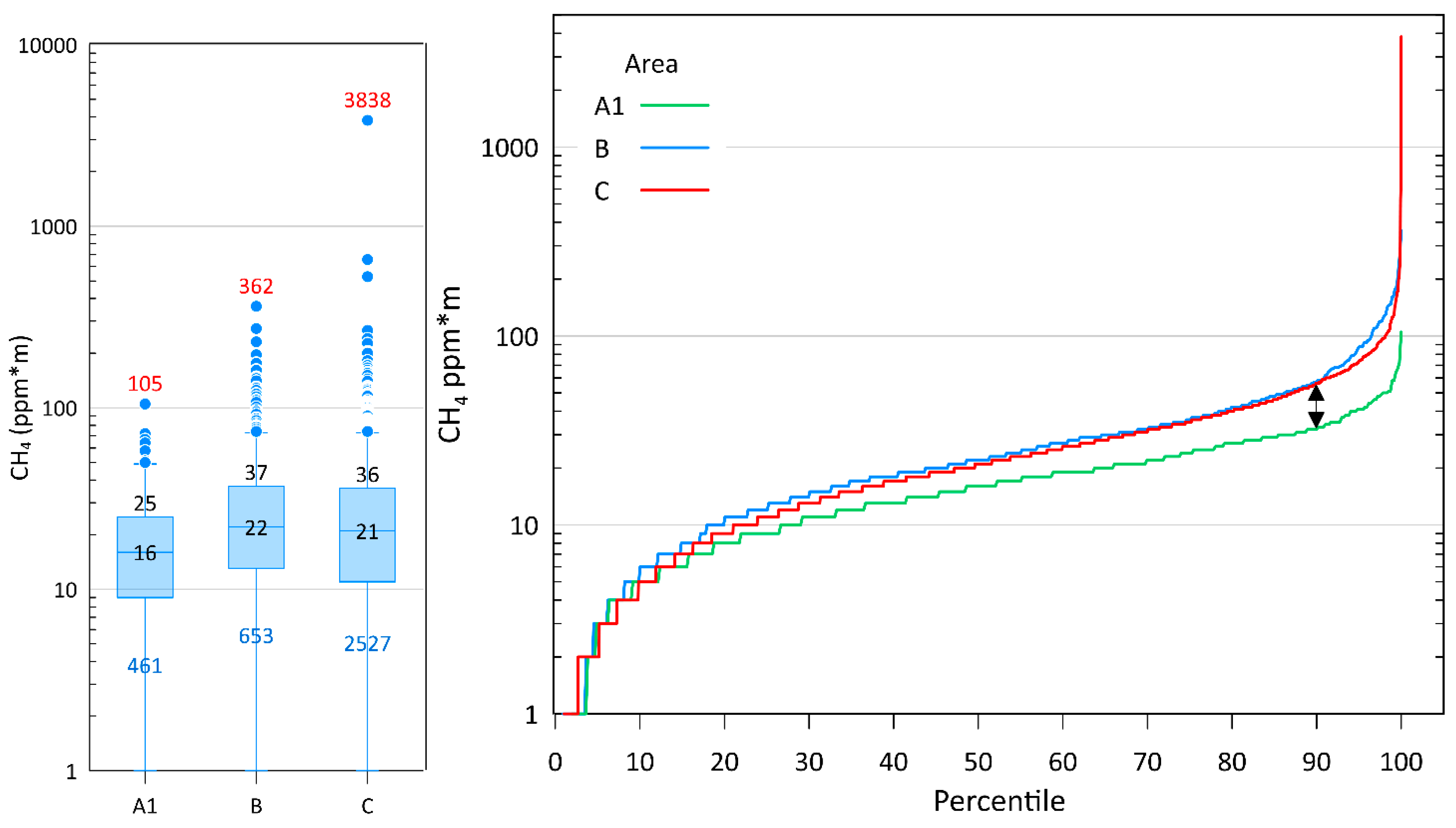
Figure 3.
Spatial distribution of CH4 (ppm*m) in area A1 (top) and area B (bottom). In area B the results of CH4 flux (mol/m2/d) measured by flux chamber are also reported.
Figure 3.
Spatial distribution of CH4 (ppm*m) in area A1 (top) and area B (bottom). In area B the results of CH4 flux (mol/m2/d) measured by flux chamber are also reported.
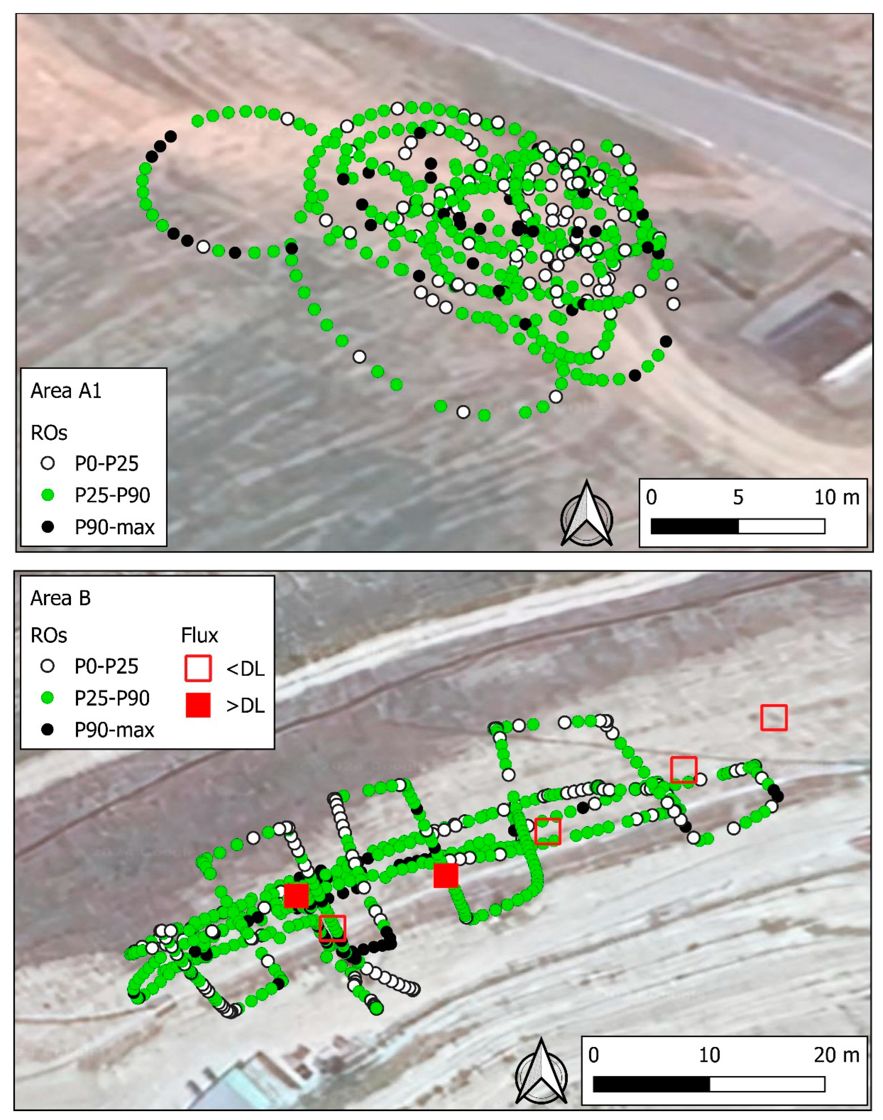
Figure 4.
Spatial distribution of CH4 (ppm*m) in area C. The result of CH4 flux (mol/m2/d) measured by flux chamber are also reported.
Figure 4.
Spatial distribution of CH4 (ppm*m) in area C. The result of CH4 flux (mol/m2/d) measured by flux chamber are also reported.
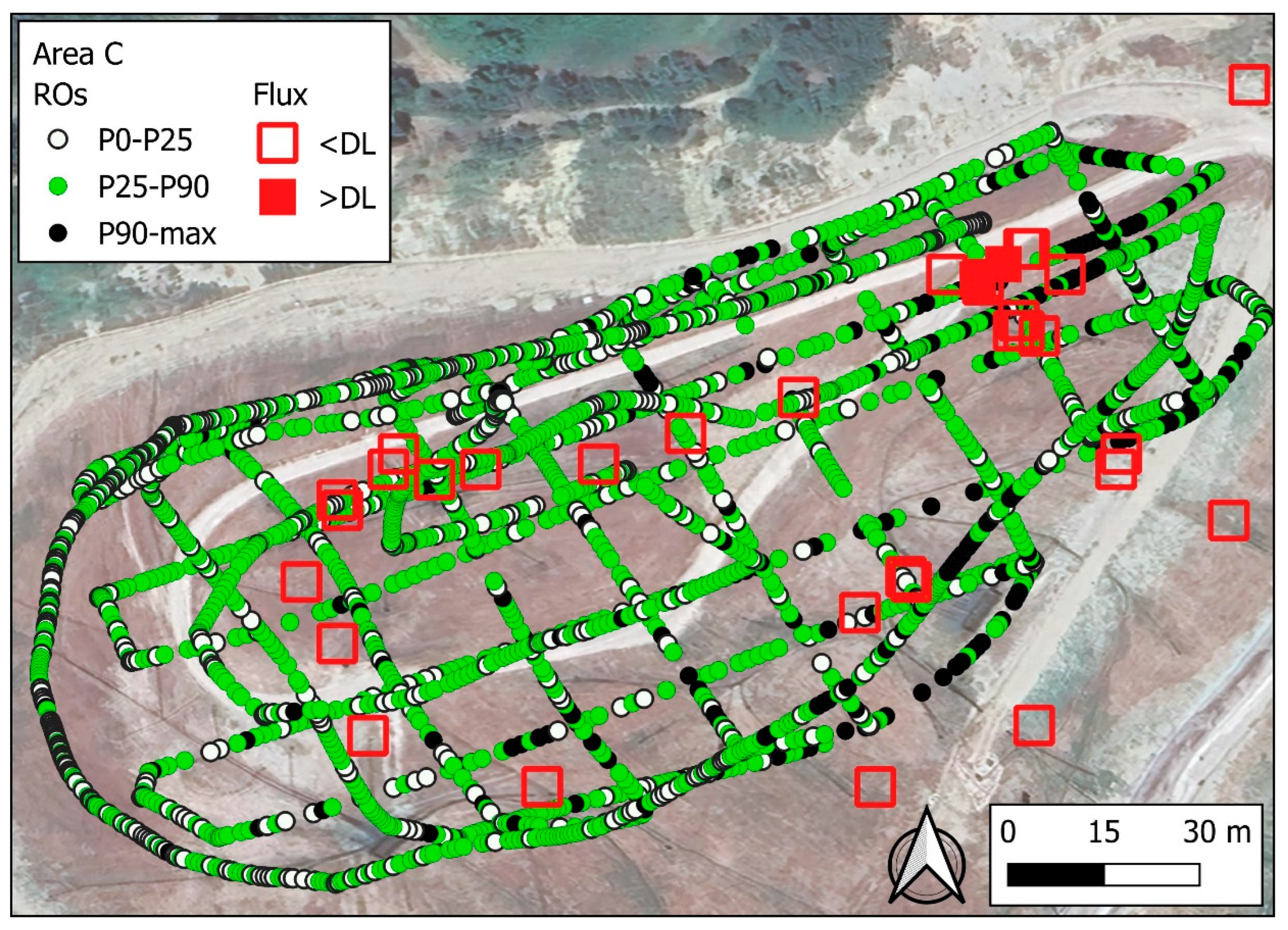
Figure 5.
General scheme of the processing of CH4 data acquired by drone. Two alternative processing are proposed. I) the raw drone-acquired observation (ROs) are grouped on a linear basis: 11 ROs acquired consecutively form an LGO (linear grouped observation), which is assigned the 75th value of the 11 ROs; ii) a variable number of ROs are grouped together as they are included in the same areal unit and form an AGO (areal grouped observation), which is assigned the average of the values of the ROs enclosed in the area. A threshold value TV (consisting of the 90th percentile of the values of LGOs and AGOs, respectively) is established. Values exceeding TVs are called HLGOs and HAGOs, respectively. The spatial contiguity of is assessed, calculating the probabilities that adjacent groups of HLGOs and HAGOs may or may not be random. The results of this evaluation are compared with CH4 flux data acquired independently with the accumulation chambers.
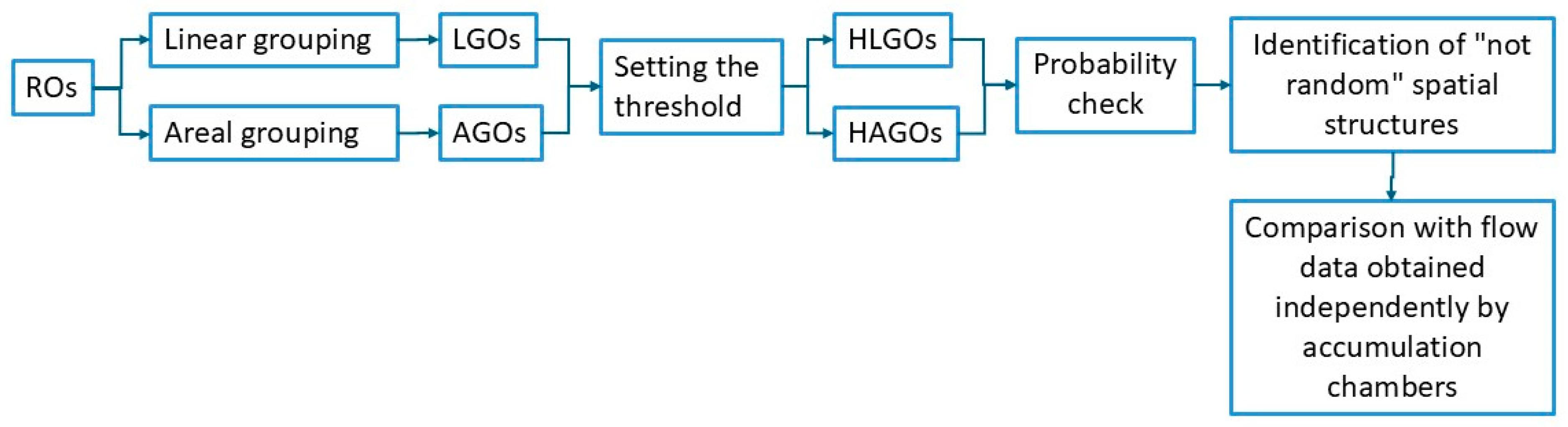
Figure 6.
CH4 distribution of LGOs and HLGOs (ppm*m) in area C. There are two lineaments formed by 4 adjacent HLGOs (yellow line) and four lineaments formed by only two adjacent HLGOs (green lines). For these latter the possibility that such structures are related to chance cannot be excluded. Results of CH4 flux (mol/m2/d) measured by flux chamber are also reported.
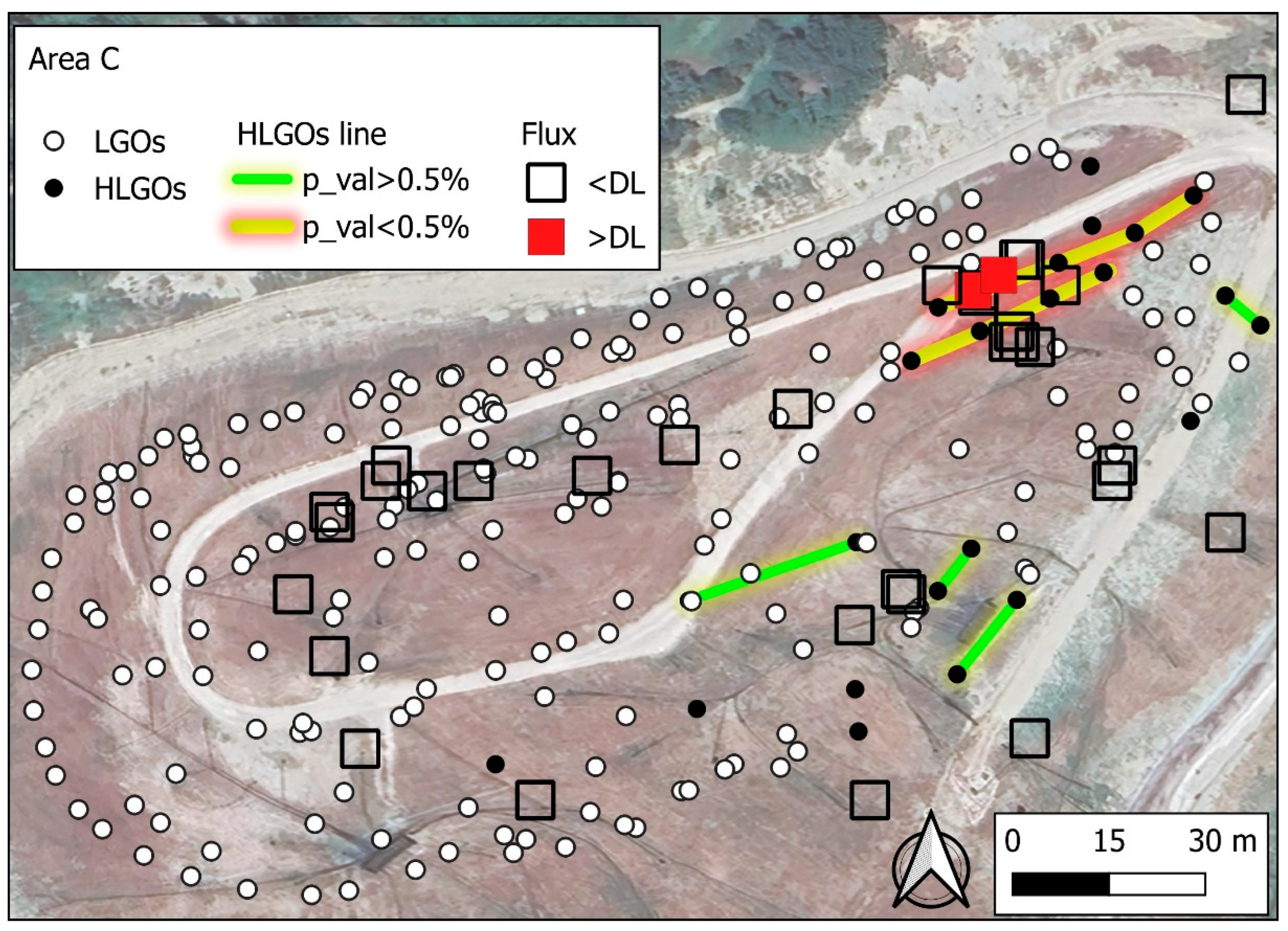
Figure 7.
CH4 distribution of LGOs and HLGOs (ppm*m) in areas A1 (top) and B (bottom). In each area there is only one lineament formed by 2 adjacent HLGOs (green line). The possibility that such structures are related to chance cannot be excluded. In the area B the results of CH4 flux (mol/m2/d) measured by flux chamber are also reported.
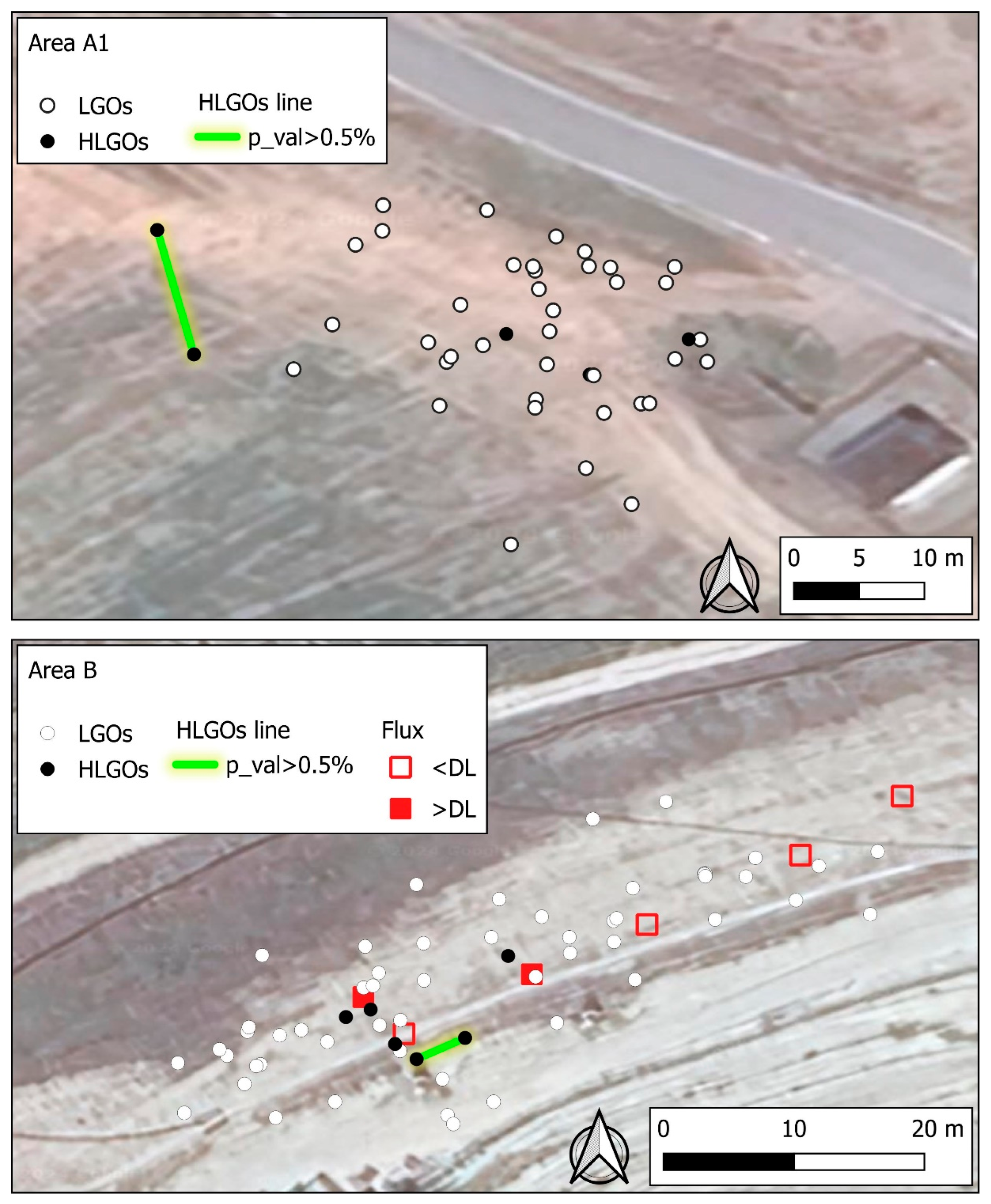
Figure 8.
ROs coverage for each AGO. The coverage is expressed as percentages related to the AGO with the highest number ROs. The numbers inside the hexagons refer to the number of ROs detected by the drone in that hexagon.
Figure 8.
ROs coverage for each AGO. The coverage is expressed as percentages related to the AGO with the highest number ROs. The numbers inside the hexagons refer to the number of ROs detected by the drone in that hexagon.
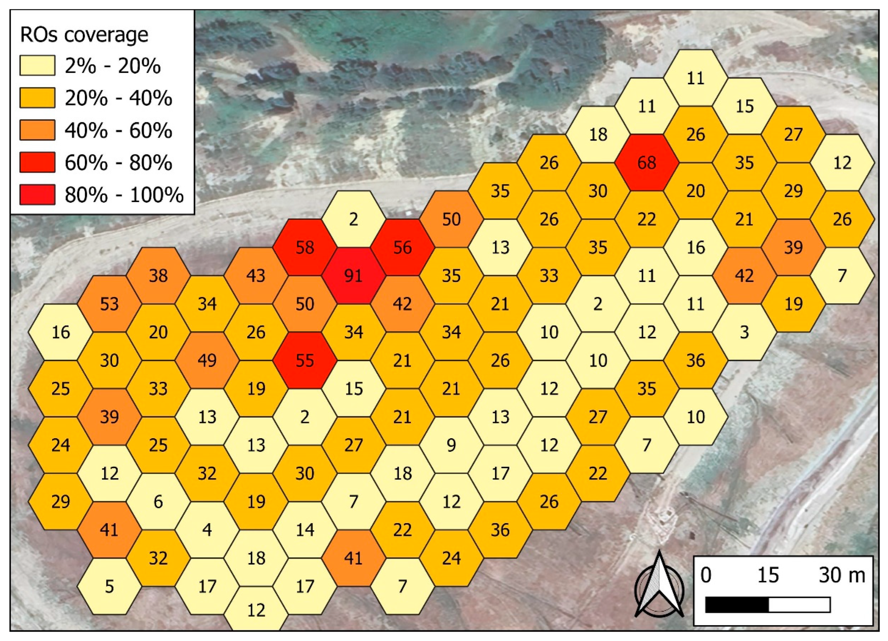
Figure 9.
Results of 2D analysis in area C. Number inside the hexagons are their Id number. Red hexagons are the HAGOs. There are two clusters of HAGOs (n. 123-132-141-142-143 and n.126-127-136). Squares are the points of CH4 flux measurements with the flux chamber. Full yellow squares represent point where CH4 flux was found greater than DL.
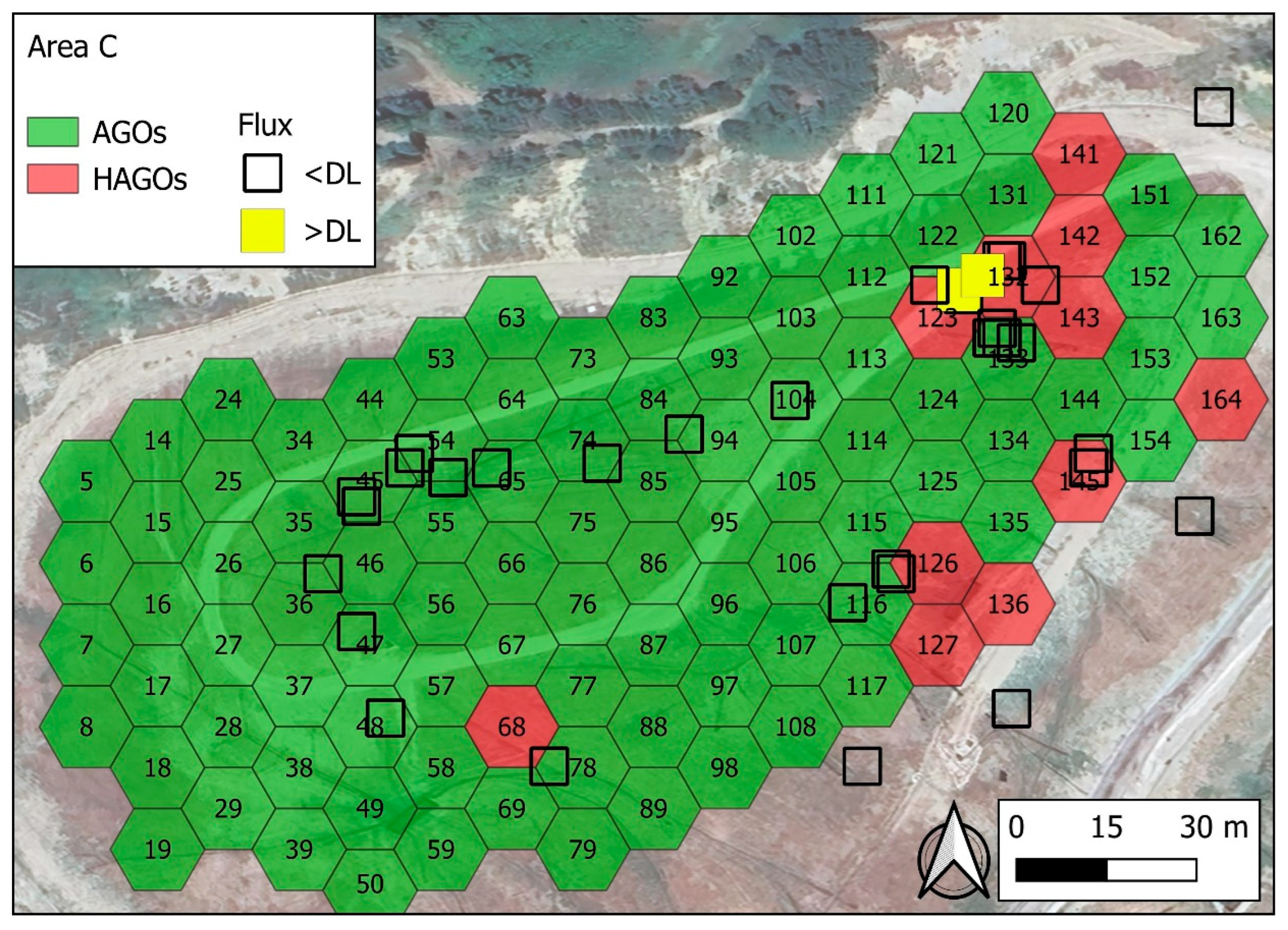
Figure 10.
Same of Figure 9; in addition, HAGOs whose clustering is poorly attributable to chance (pp_val<5%) are marked in yellow.
Figure 10.
Same of Figure 9; in addition, HAGOs whose clustering is poorly attributable to chance (pp_val<5%) are marked in yellow.
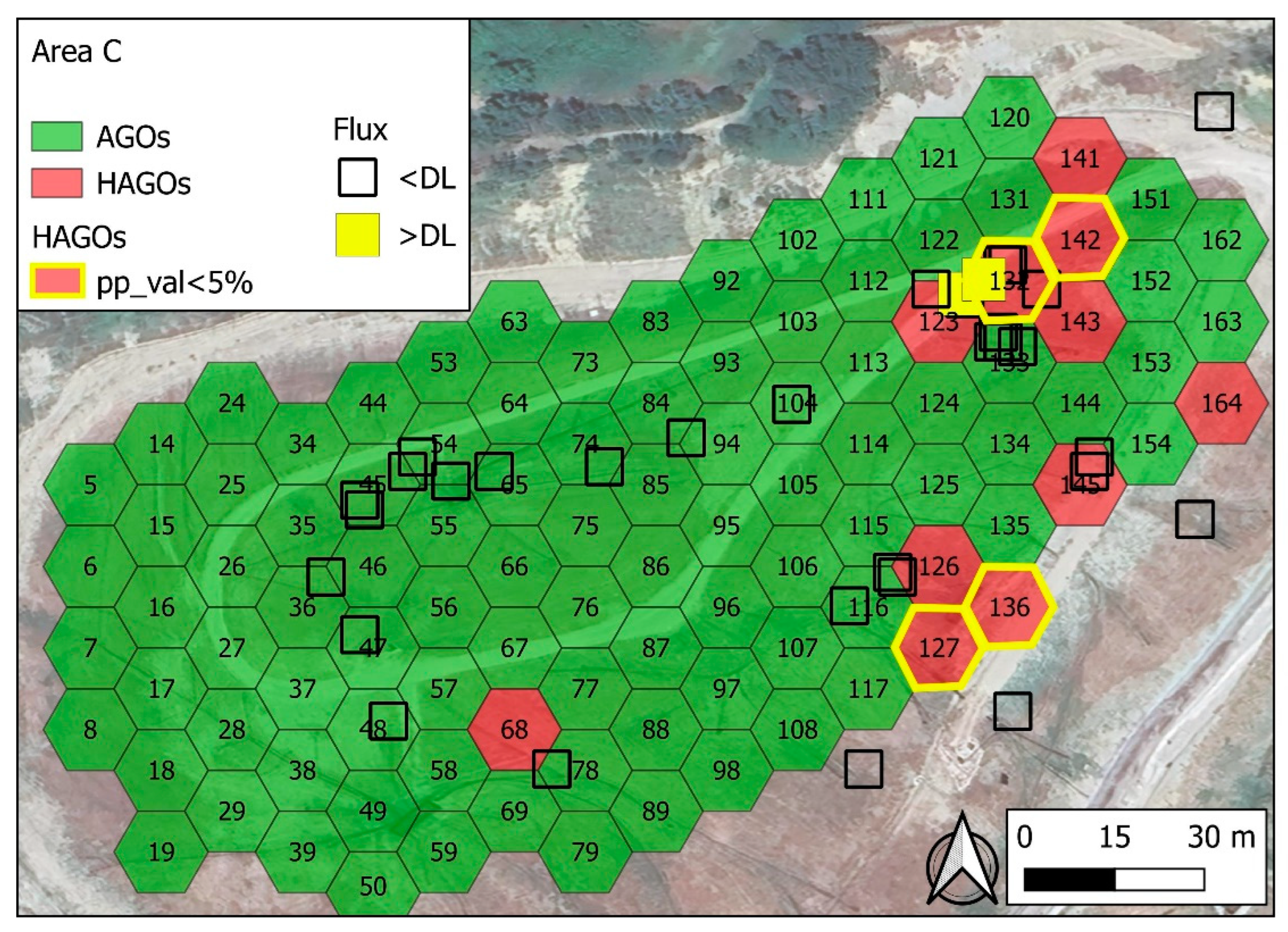
Figure 11.
Results of 2D analysis in area B. Number inside the hexagons are their Id number. Red hexagons localize the HAGOs. A 4 HAGOs (n. 50-60-61-73) cluster was tested for statistical significance. The clustering around element 61 (yellow circle) is not thought to be random but related to an emissive structure. As well this element is very close (few meters) to a measurement point where CH4 flux was clearly discernible.
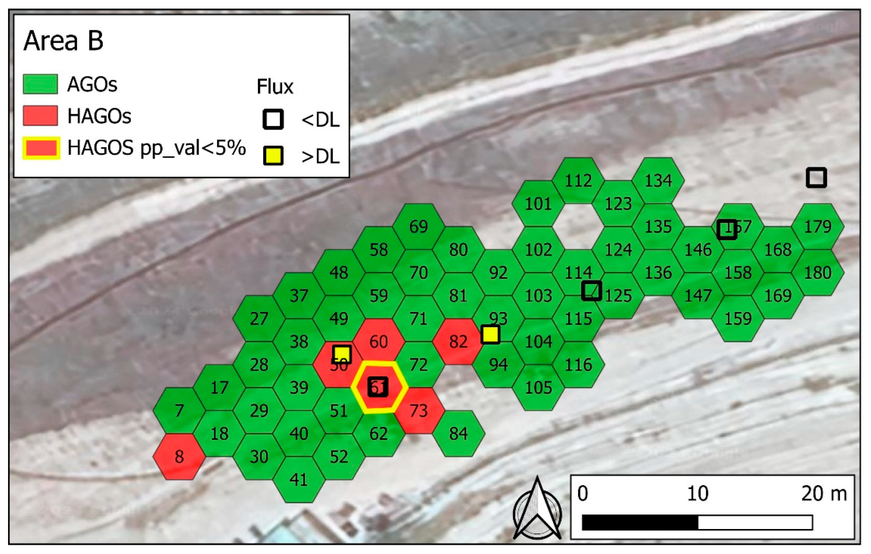
Figure 12.
Different scenarios assuming the expected relationships between UAV-sensor signal (CH4 measured in the soil-UAV column) and flux measured at the interface from the flux chambers. a) ideal conditions of no perturbation of the CH4 plume (UAV signal and flux are consistent); b) UAV-induced perturbation: the plume is displaced by downward air movement (UAV signal and flux are inconsistent); (c) windiness: perturbation giving outcomes similar to case b; (d) above-ground emission sources: CH4 plume can be detected by UAV, flux is missed by chambers. (E: emission area/point).
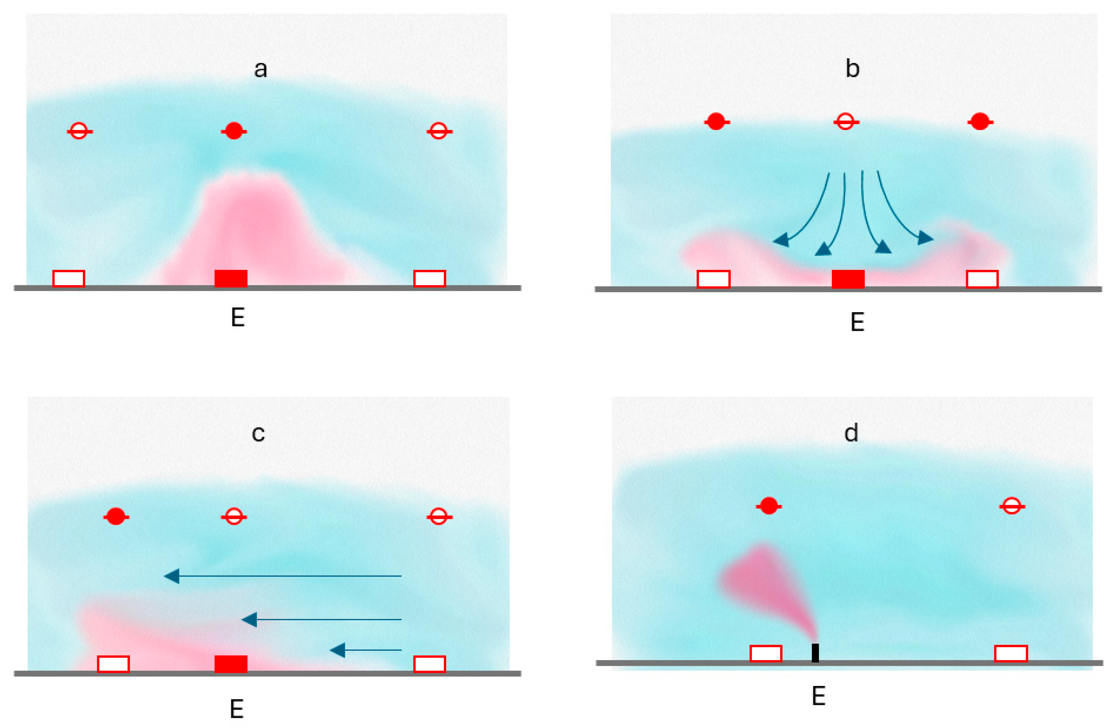
Figure 4.
Spatial distribution of AGOs and HAGOs in the area C, when varying the statistical indicator and TV. In the plots a, b, c and d the statistical indicator of AGO is respectively the mean, P50, P75 and max of ROs falling in each hexagon; the TV is set as P90 of the respective indicator (i.e. green hexagons don’t exceed the TV, red hexagon (HAGOs) do). With the same TV the HAGOs placement is roughly the same. When decreasing the TV (e.g. P90 to P75), the number of HAGOs obviously increases. The number of HAGOs with pp_val<5% seems to increase at the edge of the investigated area. The clustering centrered on HAGO n. 132 (arrow) has a pp_val<5% when TV is P90 (plot a); when TV is set to P75 (plot e) the same clustering has a pp_val>5% (as the number of HAGOS increases, the random formation of HAGOS clusters is more likely).
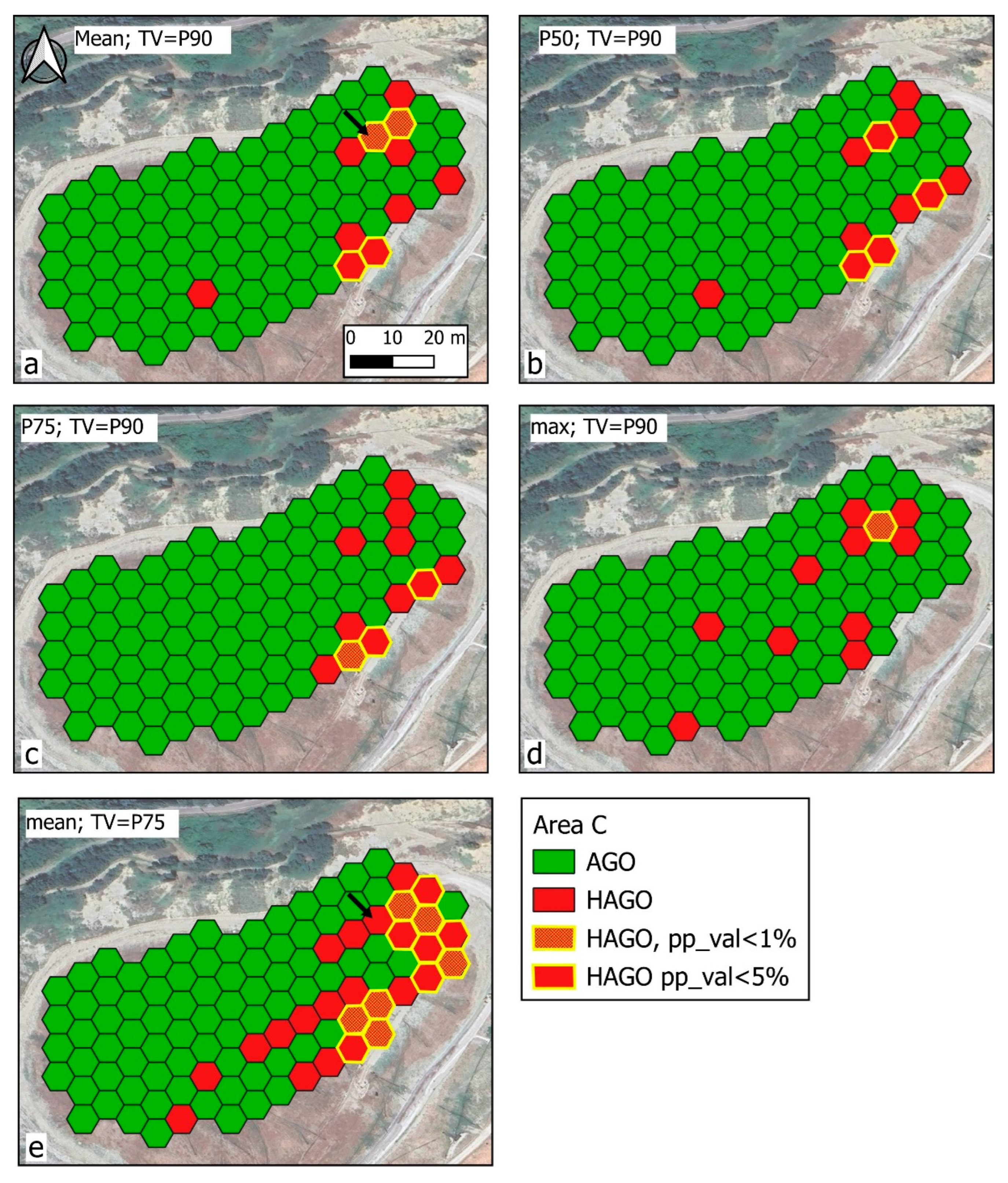
Table 1.
Sensor specifications.
| Model | PERGAM Laser Falcon |
|---|---|
| Measurement Principle | Tunable Diode Laser Absorption Spectroscopy (TDLAS) |
| Data Acquisition Frequency | 10 Hz |
| Ports | MicroUSB (power), USB (data), microSD (data) |
| Calibration | Automatic at each start-up using internal reference cell |
| Laser Footprint (Diameter) | 0.08 m at 10 m AGL, 0.18 m at 20 m AGL, 0.27 m at 30 m AGL |
| Detectability Range | 1 - 50,000 ppm *m |
| Power Supply | 5 VDC - 3° |
| Measurement Laser | 10mW Class 2 infrared laser with 1653 nm wavelength (methane selective) |
| Guidance Laser | 5mW Class 2 red laser with 532 nm wavelength |
| Sensor Dimensions | 100 × 82.5 x 80 mm |
| Mass | 0.3 kg |
| Operating Temperature Range | -17°C - +50°C |
| Operating Humidity Range | 30 - 90% |
Table 2.
Radar altimeter specifications.
| Operating Frequency | 24 GHz |
|---|---|
| Measurement Accuracy | 0.1 m |
| Communication Interface | UART |
| Measurement Range | 200 m |
| Update Rate | 50 Hz |
| Weight | 95 g |
| Dimensions | 133 71 x 16.5 mm |
Table 3.
Data Logger Specifications.
| Connections | 3 x UART, 1 x UART/RS232, 4 x GPIO pin pairs, 1 x Ethernet, 2 x USB 2.0, Bluetooth receiver |
|---|---|
| Operating Temperature Range | -25°C - +50°C |
| Input Current | 12V to 60V |
| Output Current | Selectable 9V - 12V - 15V - 18V |
| System Module | Raspberry Pi |
| RAM | 8 GB |
| Weight | 195 g |
| Dimensions | 112 x 84 x 34 mm |
Table 4.
UAV system Specifications.
| Type | Carbon fiber frame quadcopter |
|---|---|
| Power System | Dual 22.8V 6S LiPo batteries |
| Mass | 4.19 kg |
| Maximum Takeoff Weight (MTOW) | 6.14 kg |
| Propellers and Motors | 15" carbon fiber propellers |
| Dimensions | 883 × 886 × 398 mm |
| Onboard Sensors | Radar altimeter, RTK, multi-directional positioning sensors |
| Flight Software | Flight planner installed on PC and remote controller, communicating via WiFi network |
| Ingress Protection Rating | IP 43 |
| Maximum Allowable Wind Speed | 12 m/s |
Table 5.
Data acquisition pattern. Observations are provided by drone and flux chamber surveys, from investigated areas (A1, A2, B, C, see Figure 1).
Table 5.
Data acquisition pattern. Observations are provided by drone and flux chamber surveys, from investigated areas (A1, A2, B, C, see Figure 1).
|
Drone |
Site A1 (background) | CH4 (469 obs) |
|---|---|---|
| Site B (active sector) | CH4 (658 obs) | |
| Site C (capped sector) | CH4 (2552 obs) | |
|
Flux chamber |
Site A2(background) | CH4&CO2 (2 obs) |
| Site B (active sector) | CH4&CO2 (6 obs) | |
| Site C (capped sector) | CH4&CO2 (37 obs) |
Table 6.
Main statistics of data acquired by drone (ppm*m) and flux chamber (mol/m2/d). For CH4 and CO2 statistics the number in parenthesis in the “numObs” field refers to the number of observations greater than the detection limit. Out of 45 total CH4 flux measurements, only 4 were quantifiable. Therefore, for this entry, the statistics are unreliable. P10 to P99 are the respective percentiles.
| CH4(ppm*m) | N_Obs | Min | Max | Mean | P10 | P20 | P25 | P50 | P75 | P80 | P90 | P95 | P99 |
|---|---|---|---|---|---|---|---|---|---|---|---|---|---|
| A1_CH4 | 469 | 0 | 105 | 18.03 | 5 | 8 | 9 | 16 | 24 | 27 | 32 | 41 | 58 |
| B_CH4 | 658 | 0 | 362 | 30.28 | 6 | 11 | 12 | 22 | 36 | 42 | 57 | 87 | 161 |
| C_ CH4 | 2552 | 0 | 3838 | 29.04 | 5 | 9 | 11 | 21 | 35 | 40 | 56 | 73 | 126 |
| CH4 (mol/m2*d) | N_Obs | Min | Max | Mean | P10 | P20 | P25 | P50 | P75 | P80 | P90 | P95 | P99 |
| A2_ CH4_Fx | 2 (0) | 0 | 0 | 0 | n.a. | n.a. | n.a. | n.a. | n.a. | n.a. | n.a. | n.a. | n.a. |
| B_ CH4_Fx | 6 (2) | 0 | 9.235 | 2.494 | 0 | 0 | 0 | 0 | 4.298 | 5.73 | 7.483 | 8.359 | 9.06 |
| C_ CH4_Fx | 37 (2) | 0 | 3.259 | 0.132 | 0 | 0 | 0 | 0 | 0 | 0 | 0 | 0.327 | 2.673 |
| CO2 (mol/m2*d) | N_Obs | Min | Max | Mean | P10 | P20 | P25 | P50 | P75 | P80 | P90 | P95 | P99 |
| A2_CO2_Fx | 2(2) | 0.479 | 0.689 | 0.584 | 0.5 | 0.521 | 0.531 | 0.584 | 0.636 | 0.647 | 0.668 | 0.678 | 0.686 |
| B_CO2_Fx | 6 (2) | 0.264 | 6.274 | 2.244 | 0.335 | 0.406 | 0.467 | 0.985 | 3.743 | 4.551 | 5.413 | 5.843 | 6.188 |
| C_CO2_Fx | 37(35) | 0 | 1.51 | 0.238 | 0.042 | 0.071 | 0.08 | 0.172 | 0.306 | 0.333 | 0.525 | 0.639 | 1.199 |
Table 7.
Calculation of the probability (p_val%) that x HLGOs are adjacent (i.e., form a cluster) by chance, in areas C, B, A1. n: number of LGOs; h number HLGOs; x number of adjacent HLGOs.
Table 7.
Calculation of the probability (p_val%) that x HLGOs are adjacent (i.e., form a cluster) by chance, in areas C, B, A1. n: number of LGOs; h number HLGOs; x number of adjacent HLGOs.
| Area | n | h | x | Favorable cases |
Possibile cases |
p_val% |
|---|---|---|---|---|---|---|
| C | 232 | 22 | 2 | 231 | 26,796 | 0.86 |
| C | 232 | 22 | 4 | 7,315 | 117,612,110 | 0.0062 |
| B | 60 | 6 | 2 | 15 | 1770 | 0.84 |
| A1 | 44 | 5 | 2 | 10 | 946 | 1,05 |
Table 8.
Results of local joint count analysis, computed by GeoDa software. For each red hexagon in Figure 9 (i.e., hexagons where the mean value of observations detected by the drone exceeds the TV), the number of joints with other bordering red hexagons (JC) is counted. NN is the total number of joints with any other hexagon (the maximum value is 6, smaller for hexagons placed at the edges of the investigated area), pp-val% is the pseudo-probability that the JC configuration is random. pp-val% values less than 5% are marked in red.
| Id_exagon | JC | NN | pp_val% |
|---|---|---|---|
| 123 | 1 | 6 | 46.5 |
| 126 | 2 | 6 | 9.6 |
| 127 | 2 | 4 | 4.1 |
| 132 | 3 | 6 | 0.9 |
| 136 | 2 | 3 | 2.7 |
| 141 | 1 | 4 | 33.3 |
| 142 | 3 | 6 | 1.1 |
| 143 | 2 | 6 | 09.2 |
Disclaimer/Publisher’s Note: The statements, opinions and data contained in all publications are solely those of the individual author(s) and contributor(s) and not of MDPI and/or the editor(s). MDPI and/or the editor(s) disclaim responsibility for any injury to people or property resulting from any ideas, methods, instructions or products referred to in the content. |
© 2025 by the authors. Licensee MDPI, Basel, Switzerland. This article is an open access article distributed under the terms and conditions of the Creative Commons Attribution (CC BY) license (http://creativecommons.org/licenses/by/4.0/).
Copyright: This open access article is published under a Creative Commons CC BY 4.0 license, which permit the free download, distribution, and reuse, provided that the author and preprint are cited in any reuse.


