
Submitted:
21 April 2025
Posted:
27 April 2025
You are already at the latest version
Abstract
The GM(1,1) model is a well-established model for time series forecasting, particularly effective for systems with limited data and poor information. However, its performance often degrades in dynamic systems, leading to significant prediction errors. To address these challenges, we propose an Elastic Optimal Adaptive GM(1,1) Model, dubbed as EOAGM, to improve forecasting performance. Specifically, our proposed EOAGM dynamically optimizes the sequence length by discarding outdated data and incorporating new data, therefore reducing the influence of irrelevant historical information. Moreover, we introduce a stationarity test mechanism to identify and adjust sequence data fluctuations, ensuring stability and robustness against volatility. Additionally, the model refines parameter optimization by incorporating predicted values into candidate sequence and assessing their impact on subsequent forecasts, particularly under conditions of data fluctuation or anomalies. Experimental evaluations demonstrate the superiority of our model on prediction precision and reliability on multiple real datasets over six baseline competitors.
Keywords:
stationarity test
; elastic adjustment
; optimal adaptation
; GM(11)
1. Introduction
Time series analysis, recognized as a core research direction in the field of data mining, is considered one of the top ten technical challenges of the 21st century [1,2]. At its core, time series forecasting leverages historical data to uncover temporal patterns, constructing predictive models that provide quantitative foundations for trend anticipation, risk early warning, and evidence-based decision-making [3,4,5]. Research indicates that effective time series forecasting not only reveals the evolution mechanisms of systems [6,7,8], but also offers technological support for industrial upgrading, thereby facilitating the implementation of cross-industry sustainable development strategies [9,10].
Among various forecasting methods [11,12,13], the GM(1,1) model has garnered significant attention due to its unique capability in small-sample modeling [14,15]. As an important tool in grey system theory, this model demonstrates significant advantages in system behavior modeling and evolution analysis through specialized data generation mechanisms with limited information [16,17]. Its core features are: (1) modeling with as few as four data points; (2) no preset distribution assumptions; (3) a combination of computational efficiency and verifiability. These characteristics have enabled its application across a wide range of fields. For instance, Cai et al. [18] employed an enhanced GM(1,1) model to predict economic losses caused by marine disasters, while Ding [19] used a self-adaptive intelligent grey model to forecast natural gas demand.
However, the classical GM(1,1) model still faces significant challenges in predicting dynamic systems [20,21]: First, the traditional accumulation generation mechanism struggles to capture temporal fluctuation characteristics; Second, the fixed-length modeling window fails to adapt to changes in data distribution; Third, the parameter optimization process lacks dynamic error correction mechanisms [22]. Although existing studies have improved model performance through refinements of background values, construction of grey derivatives, and parameter optimization [23,24], most methods still assume system stability and do not effectively address data fluctuation issues in dynamic environments.
To overcome the challenges encountered by the traditional GM(1,1) model in dynamic system forecasting, we propose an innovative Elastic Optimal Adaptive GM(1,1) Model (EOAGM). This model enhances performance through three key innovations: First, it replaces the traditional cumulative generation sequence with an adaptive sequence generation method, strengthening the influence of recent observations and enhancing the model’s ability to capture dynamic system characteristics. Second, it introduces a statistical stationarity test framework to establish a dynamic adjustment mechanism for sequence length, enabling a transition from fixed windows to elastic ones. Lastly, it constructs a candidate sequence evaluation system that incorporates predicted values for back-validation and optimal sequence selection, forming a closed-loop optimization system for error self-correction, effectively improving the model’s predictive performance. These improvements significantly enhance the model’s adaptability and accuracy in dynamic systems, achieving superior simulation and forecasting outcomes. The contributions of our work could be summarized as follows:
- Adaptive Sequence Generation Mechanism: We have improved the architecture of the grey system model by employing an adaptive sequence generation method that integrates the accumulation of historical data with the timing of recent observations. This enhanced framework effectively captures and characterizes the inherent complex temporal patterns in the system’s evolution by strengthening the dynamic representation of temporal features.
- Elastic Modeling Window: We have integrated stationarity testing into the grey system to dynamically adjust the sequence length used for prediction within the grey system. This reduces the adverse impact of changes in data distribution on prediction accuracy.
- Candidate Sequence Evaluation System: We propose an optimal sequence selection method to evaluate whether replacing actual values with predicted values can improve the accuracy of sub-sequent predictions. The optimal sequence is then chosen to dynamically correct the prediction errors.
- Applications and validation: The proposed model was applied to forecast dynamic systems, including China’s GDP and indigenous thermal energy consumption. Comparative analysis against other models revealed that our approach delivers superior predictive accuracy for dynamic systems.
2. Related Work
The grey forecasting model GM(1,1), introduced by Deng in 1982 [25], provides a robust framework for time series forecasting under incomplete information conditions. Renowned for its high precision and computational simplicity, the GM(1,1) model has been extensively adopted across various domains. It operates on the principle of interactive computation, leveraging limited and incomplete data during both model construction and parameter optimization. This involves formulating a first-order differential equation derived from the accumulated generating sequence, capturing the system’s development trends, with parameter estimation performed using statistical techniques like least squares. The model’s mechanism comprises three key steps:
- Accumulated Generating Operation (AGO): The original dataset undergoes an accumulated transformation to yield a new sequence, emphasizing the system’s development trend and rendering the data’s evolution more discernible.
- A first-order linear differential equation is constructed based on the accumulated sequence, describing the data’s progression. Parameters are estimated using statistical methods, such as the least squares method.
- Optimization focuses on estimating the development coefficient and other parameters critical for the model’s accuracy.
Researchers have worked extensively to refine the GM(1,1) model by optimizing background values, grey derivatives, and parameter estimation processes [26,27,28]. Enhancements in the background value calculation have significantly improved prediction precision. For instance, Zhan et al [29] developed a multi-parameter background value approach for nonlinear optimization, while Ma and Wang [30] proposed background value optimization based on improved algorithms. Similarly, Approximation of piecewise linear and generalized functions can be used for constructing background values to improve accuracy. Grey derivative calculations, crucial for capturing trends in data, have also seen advancements [31,32,33]. Parameter optimization remains a cornerstone for ensuring the GM(1,1) model’s robustness [34]. Despite these advancements, the GM(1,1) model’s assumption of system stability often limits its performance when applied to datasets characterized by high volatility or dynamic behavior [35].
Adaptive parameter estimation methods have been proposed to address these challenges, enabling real-time parameter adjustment based on incoming data. However, such kind of approaches often overlook the role of sequence stability in improving predictions [36]. Sequence stationarity, a fundamental prerequisite in time series forecasting, is essential for ensuring reliable and interpretable predictions. Stationarity detection methods, such as the Augmented Dickey Fuller (ADF) test [37,38], the Kwiatkowski-Phillips-Schmidt Shin (KPSS) test [39,40], and the Phillips-Perron (PP) test [41,42], are widely used to evaluate unit roots or trends in datasets. Correctly addressing non-stationarity through techniques like differencing or detrending, enhances a model’s ability to capture underlying patterns and produce robust fore-casts. Despite these efforts, the fixed-length sequence framework of traditional grey systems, which retains recent data and discards older data, often fails to maintain sequence stability in dynamic environments. To overcome these limitations, we propose the EOAGM. This innovative model dynamically adjusts the data sequence length, discarding outdated information while integrating new data, thereby reducing the influence of irrelevant historical data. A stationarity test is incorporated to detect sequence fluctuations and dynamically modify sequence length, enhancing robustness against data volatility. Furthermore, parameter optimization is refined by integrating predicted values into candidate sequence, enabling the evaluation of their efficacy in subsequent forecasts. This strategy improves the model’s adaptability and precision in capturing patterns within dynamic systems, achieving superior simulation and forecasting performance.
3. Materials and Methods
3.1. Traditional GM(1,1) Model
The key steps of the traditional GM(1,1) model (TGM) are as follows: Let the time series have n observations, , by AGO, we generate a new sequence , , where
The adjacent mean generation sequence of is computed as:
Then the model establishes the first-order linear differential equation:
Where is the developmental gray number, and the is the endogenous control gray number. The parameters and are estimated using the least squares method:
where
The prediction model derived from the differential equation is:
From this, the predicted values for the original sequence are obtained as:
3.2. The Elastic Optimal Adaptive GM(1,1) Model
The The Elastic Optimal Adaptive GM(1,1) model (EOAGM) enhances the prediction accuracy of grey systems through parameter optimization methods. As illustrated in Figure 1, the EOAGM model is structured into three main steps:
- Sequences Construction: This step involves generating two types of sequences, the original sequence and the candidate sequence, to ensure robust prediction capability.
- Stationarity Detection: The EOAGM model improves on the AGM by using the ADF test to evaluate the stability of sequences. Stationarity ensures the model’s parameters accurately represent the system’s behavior, leading to better prediction accuracy.
- Optimal Sequence Selection: This step identifies the sequence that provides the best prediction accuracy by evaluating the performance of both original and candidate sequences.
3.2.1. Sequences Construction
The process of sequences construction involves generating the original sequence and the candidate sequence, each designed to optimize prediction performance. The steps include:
- Defining Sequence Length: The optimal length is set for both the original and candidate sequences.
- Data Insertion: When the sequence length is not more than , new data points are directly added to both sequences. When the sequence length exceeds , the observed value is appended to the original sequence, while the predicted value is added to the candidate sequence.
- Maintaining Sequence Length: To keep the sequence length fixed, the oldest value is discarded from both sequences.
- Temporary Storage of Discarded Values: Discarded values are stored temporarily, allowing the model to revert to previous states during the stationarity detection phase if instability is detected. This structured approach ensures the sequences are robust, adaptable, and ready for subsequent stationarity detection and optimization steps.
3.2.2. Stationarity Detection
In the AGM, the length of the data sequence used to calculate the model parameters and is fixed. However, even with operations that involve discarding outdated data and incorporating new data, the sequence stability may still degrade, leading to poor model performance and inaccurate predictions. To address this limitation, we introduce the ADF test method to assess the stability of the sequence within the model.
ADF test is a statistical method used to determine whether a time series has a unit root, which indicates non-stationarity. When conducting an ADF test, we typically pay attention to the test statistic (), the probability of the sequence being non-stationary (), and the critical values () associated with the confidence interval.
The ADF test indicates whether the sequence has a unit root. A smaller than the implies stationarity. measures the probability of the sequence being non-stationary, with a indicates stationarity. The ADF test results provide at different confidence levels (e.g., 1%, 5%, 10%), which are used to compare with the [43]. In the ADF test, the critical values of the confidence interval help us determine whether the time series is stationary, rather than directly providing a confidence interval for a parameter.
The procedure for calculating ADF statistics to test for the presence of unit roots is shown in Equation 7.
In the traditional DF test, the value of the time series at time t is denoted as , the first-order difference of the series at time is denoted as , and the difference term is . In the traditional DF detection, an enhancement is made, transforming as shown in Equation 8.
Thus, the ADF formula can be transformed into:
The calculated test statistic is obtained as:
Modern statistical tools such as R, Python, Stata, and EViews can automatically match the appropriate Dickey-Fuller distribution table based on the sample size and the number of lag terms, providing the corresponding and as outputs. This ensures accurate results tailored to the specific characteristics of the dataset being analyzed.
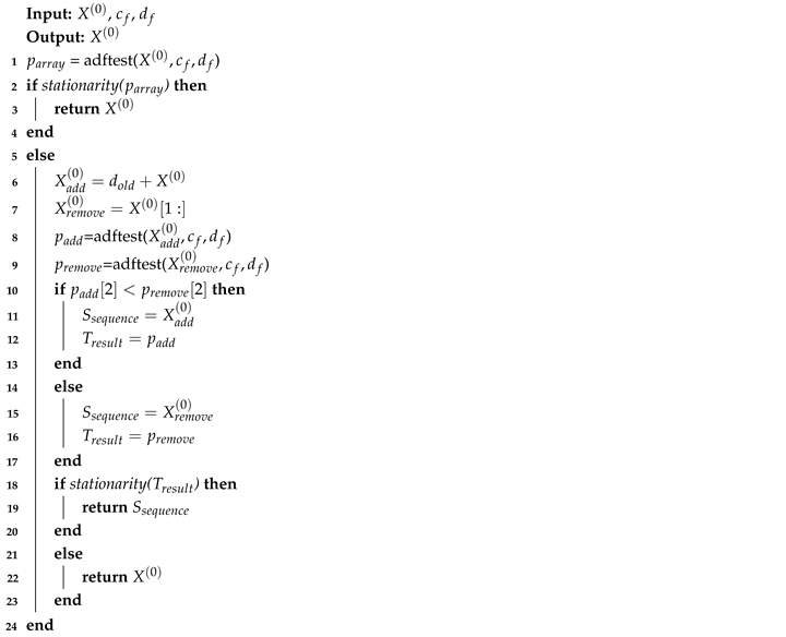
Using the ADF test, we assess whether adaptive adjustments to the sequence maintain its stability. Based on the test results, decisions can be made to modify the sequence length if necessary. If the adjusted sequence fails to achieve stationarity, the original sequence length is preserved. The elastic adjustment process, as outlined in Algorithm 1, incorporates several parameters: , representing the confidence level (e.g., 1%, 5%, or 10%, corresponding to 99%, 95%, and 90% probabilities of stationarity, respectively); And [44], indicating the differencing order, which can be first-order or second-order differencing for non-stationary time series data [45]. The ADF test method is applied to the sequence, yielding a result array containing , and , which collectively determine stationarity. To evaluate this, the stationarity method examines the array: if and , the sequence is deemed stationary; Otherwise, it is considered non-stationary. For non-stationary sequences, adjustments involve creating two new sequences (one by adding a data point to the beginning of the original sequence and the other by removing the oldest data point) and applying the ADF test to both. The sequence with the smaller is selected for further evaluation using the stationarity method. If the sequence achieves stationarity, it is used for subsequent modeling; Otherwise, the original sequence is retained. This iterative approach ensures the balance and robustness of the sequence for accurate forecasting.
| Algorithm 1: elastic adjustment process |
 |
3.2.3. Optimal Sequence Selection
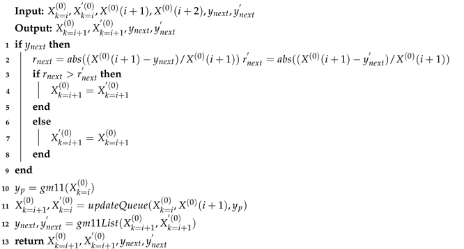
Stationarity detection adjusts the sequence length by adding or removing data from the sequence’s head to achieve a stable state. However, the sequence accepts all newly added values, including outliers or values with significant fluctuations, which would reduce the accuracy of the forecast result. Therefore, we employ the Optimal Sequence Selection method to enhance prediction accuracy. The Optimal Sequence Selection method is described in Algorithm 2. In Algorithm 2, we add a candidate series. Let the original series be a time series with i observations, At the moment , we obtain , which is added to the original series and discard the oldest data to obtain a new series , which serves as a prediction sequence, which is consistent with the AGM. In addition, we add the candidate series .
At the moment , we compare the true values with the predicted values of the two series, and thus select a series with a small relative error, and then add new data, discard the old data, and generate a new candidate series right on top of the selection sequence.
The most useful thing about the candidate series is that the better data among the predicted data and the real data is selected for prediction, which leads to better prediction results.
| Algorithm 2: Optimal Sequence Selection |
 |
4. Experimental Results and Discussion
In this study, we first present the datasets, baseline methods, and evaluation metrics. Subsequently, we compare the prediction accuracy across different baseline approaches. Next, we conduct a sensitivity analysis to assess model robustness. Finally, we perform an ablation experiment to evaluate the contribution of key components.
Datasets :To validate the superiority of our algorithm, we conducted experiments on two distinct datasets: (1) China’s annual GDP data from 2008 to 2023, and (2) district heating data from Jinan City, China. For the GDP dataset, obtained from the National Bureau of Statistics of China (https://data.stats.gov.cn/), we utilized observations from 2008–2014 (31.92, 34.85, 41.21, 48.79, 53.86, 59.30, and 64.36 trillion yuan) as the training set to predict subsequent years’ values (2015–2021: 68.89, 74.64, 83.20, 91.93, 98.65 and 101.60 trillion yuan). For the heating dataset, we selected daily measurements from six residential buildings during January 1–13. The model was trained on data from January 1–7 and tested on its ability to forecast heating demand for January 8–13. The raw district heating data are presented in Table 1. Column 1 represents observation dates and columns 2-7 represent daily thermal energy consumption (kWh) for Buildings 11-16.
Baseline Method :In addition to the traditional GM(1,1) (TGM), this study cbomprehensively evaluates five advanced grey models and one non-grey model proposed in recent literature.
- Cumulative GM(1,1) Model (CGM)[46]: The CGM recalculates and iteratively by incorporating new data. While this method improves adaptability by considering growing datasets, the increasing sequence length may introduce noise and irrelevant information, reducing prediction precision over time.
- Adaptive GM(1,1) Model (AGM) [47]: The AGM dynamically adjusts the data sequence by discarding older data and incorporating new observations. This approach enhances forecasting accuracy for dynamic systems by reflecting real-time changes. However, removing older data may destabilize predictions, and incorporating new data (including anomalies) may reduce prediction reliability.
- Simultaneous Grey Model (SimGM) [35]: This model can improve the algorithm for calculating and [48]. Traditional GM(1,1) employs ordinary least squares (OLS) to estimate and . However, since real-world systems are governed by interconnected and evolving factors, a single differential equation may inadequately capture these relationships. To address this limitation, the SimGM has been proposed, which significantly improves prediction accuracy compared to conventional single-equation models.
- Nonlinear Grey Model (NonlGM) [49]: The NonlGM proposes an enhanced GM(1,N) model incorporating nonlinear optimization techniques to improve forecasting accuracy and robustness. The background value in the TGM(1,1) model is defined as . In the process of background value optimization, The fixed weight coefficient (0.5) can be optimized. In the NonlGM, , where a is optimized.
- Improved Grey Model (ImGM) [30]: This model is an improved optimized background value determination method for the GM(1,1) model. In this method, background value optimization can also be achieved through exponential background value and dynamic adaptive background value using data characteristics methods.
- Laggred [50]: This model employs a non-grey modeling approach for data forecasting, specifically utilizing a quantile regression framework with lagged and asymmetric effects.
Evaluation Metrics :In the experiment, relative error and mean error are used as test indicators. The formula for calculating relative error is as follows:
Where is the predicted value of the k-th data point, is the true value of the k-th data point. Assuming n is the number of predicted values, then the average error of the prediction is:
Sequence Length Setting :Experimental results demonstrate that setting the sequence length to 7 yields the minimal prediction error for EOAGM when forecasting both China’s GDP and Jinan’s thermal energy consumption data.
ADF Method Parameter Settings :
The sequence is considered stationary when the (probability of the observed sequence) < 0.05 and the test statistic () < the critical value (). Since critical values are provided at three confidence intervals, appropriate selection of the confidence level is required.
Considering the inherent stability of thermal energy consumption data compared to GDP data which is subject to multiple influencing factors, we adopted distinct confidence levels: 99% confidence interval for thermal energy consumption forecasting versus 90% for GDP prediction.
Similarly, regarding the differencing order in the Augmented Dickey-Fuller (ADF) test, first-order differencing was applied to thermal energy consumption data while second-order differencing was implemented for GDP data.
4.1. Performance Comparison with Base Lines
4.1.1. National GDP Prediction
To validate the universal applicability of our proposed model, we conducted comprehensive predictions of China’s GDP from 2015 to 2021 using eight grey models: TGM/CGM/AGM/SimGM/ NonlGM/ImGM/Lagreg and EOAGM.
The errors of each model for different years, as well as the mean errors, are presented in Table 2. As can be observed from Table 2, our algorithm achieves the smallest values in both mean error and maximum error.
Furthermore, a line chart (Figure 2) was employed to illustrate the stability of the algorithms. The yellow line represents the error trend of our proposed algorithm, demonstrating its exceptional stability.
4.1.2. Indigenous Thermal Energy Prediction
The TGM/ CGM/ AGM/ and EOAGM were applied to forecast indigenous thermal energy prediction for six buildings over the period from January 8th to January 13th. The corresponding prediction errors are visualized in Figure 3.
As shown in Figure 3, both the AGM and the EOAGM outperform the TGM and CGM. Furthermore, the EOAGM consistently surpasses the adaptive model in prediction accuracy,
Using the mean error as a test indicator for the four algorithms, as shown in Table 3, except for Building 11, the average error of the EOAGM is the smallest in the other five buildings. Moreover, if the data fluctuates or there are anomalous data, the prediction accuracy of the EOAGM will be significantly improved.
4.1.3. On Model Comparison
As demonstrated in Table 2 and Table 3, the proposed EOAGM model exhibits superior performance compared to the seven baseline methods. This enhanced performance can be attributed to the following key innovations:
Stability-Aware Adaptive Forecasting:The model incorporates stationarity testing and dynamic sequence length adjustment, effectively mitigating prediction errors caused by temporal fluctuations. This ensures robust performance under non-stationary conditions.
Predictive Parameter Optimization:A novel parameter optimization strategy is implemented by embedding predicted values into candidate sequences. This approach allows for direct evaluation of their predictive efficacy in subsequent forecasting steps, thereby enhancing both adaptability and precision in dynamic system modeling.
4.2. Ablation Experiment
In this section, we perform necessary ablation studies through removing specific components to generate three ablation models.
1. EOAGM-A: We replace the dynamic adaptive adjustment of sequences with a cumulative aggregation mode for data prediction.
2. EOAGM-O: We remove the optimal sequence selection for data prediction.
3. EOAGM-E: We omit the stationarity detection for data prediction.
As can be seen from Table 4, removing one of the three components affects the accuracy of the algorithm’s prediction.
5. Conclusion
To address the challenges of unstable prediction accuracy and susceptibility to noise interference in the TGM, this study proposes the EOAGM, an enhanced version of the AGM. Firstly, we replace the traditional cumulative generation sequence with an adaptive sequence generation method, which enhances the model’s ability to manage dynamic time series. Secondly, a stationarity detection method is introduced to adjust the sequence length dynamically, shifting from fixed-length to elastic sequences to reduce the impact of data fluctuations. Finally, the parameter optimization process is improved by incorporating predicted values into the candidate sequence. This allows for evaluating whether the inclusion of predicted values in subsequent forecasts improves performance, particularly in the presence of data volatility or anomalies. By selecting the optimal sequence, the proposed model significantly improves both simulation accuracy and predictive precision. The EOAGM has already been successfully applied to the Jinan Municipal Thermal Energy System, yielding positive outcomes. Future work will focus on further enhancements, including optimizing the background value and incorporating second-order residual correction, to achieve even greater prediction accuracy and robustness.
Author Contributions
Conceptualization, T.L. and Z.L.; methodology, T.L. and Z.L.; software, T.L and J.N.; validation, G.Q., T.L. and C.J.; formal analysis, Q.L. and Z.L.; investigation, Q.L. and Z.L.; resources, Q.L. and Z.L.; data curation, T.L.; writing—original draft, C.J.; writing—review and editing, G.Q.; visualization, T.L.; supervision, J.N. and Z.L.; project administration, T.L. All authors have read and agreed to the published version of the manuscript.
Funding
This research was funded by the National Natural Science Foundation of China grant number 62276155 and 62206157
Data Availability Statement
The data presented in this study are available on request from the corresponding author.
Acknowledgments
The authors are grateful to the editor and reviewers for their constructive comments, which have significantly improved this work.
Conflicts of Interest
The authors declare no conflicts of interest.
References
- Alqahtani, A.; Ali, M.; Xie, X.; Jones, M. Deep Time-Series Clustering: A Review. Electronics 2021. [Google Scholar] [CrossRef]
- Liu, F.; Chen, L.; Zheng, Y.; Feng, Y. A Prediction Method with Data Leakage Suppression for Time Series. Electronics (2079-9292) 2022, 11. [Google Scholar] [CrossRef]
- Liu, F.; Yin, B.; Cheng, M.; Feng, Y. n-Dimensional chaotic time series prediction method. Electronics 2022, 12, 160. [Google Scholar] [CrossRef]
- Wan, R.; Tian, C.; Zhang, W.; Deng, W.; Yang, F. A multivariate temporal convolutional attention network for time-series forecasting. Electronics 2022, 11, 1516. [Google Scholar] [CrossRef]
- Kim, M.; Lee, S.; Jeong, T. Time series prediction methodology and ensemble model using real-world data. Electronics 2023, 12, 2811. [Google Scholar] [CrossRef]
- Yuan, H.; Liao, S. A time series-based approach to elastic kubernetes scaling. Electronics 2024, 13, 285. [Google Scholar] [CrossRef]
- Li, G.; Yang, Z.; Wan, H.; Li, M. Anomaly-PTG: a time series data-anomaly-detection transformer framework in multiple scenarios. Electronics 2022, 11, 3955. [Google Scholar] [CrossRef]
- Zhong, Y.; He, T.; Mao, Z. Enhanced Solar Power Prediction Using Attention-Based DiPLS-BiLSTM Model. Electronics 2024, 13, 4815. [Google Scholar] [CrossRef]
- Ma, X.; Chang, S.; Zhan, J.; Zhang, L. Advanced Predictive Modeling of Tight Gas Production Leveraging Transfer Learning Techniques. Electronics 2024, 13, 4750. [Google Scholar] [CrossRef]
- Dai, L.; Liu, J.; Ju, Z. Attention Mechanism and Bidirectional Long Short-Term Memory-Based Real-Time Gaze Tracking. Electronics (Switzerland) 2024, 13, 4599. [Google Scholar] [CrossRef]
- Liu, Q.; Hu, Y.; Liu, H. Ensemble Forecasting of Stock Prices using Multidimensional Grey Model and ATT-LSTM with Multi-source Heterogeneous Data. IEEE Access 2024. [Google Scholar] [CrossRef]
- Masini, R.P.; Medeiros, M.C.; Mendes, E.F. Machine learning advances for time series forecasting. Journal of economic surveys 2023, 37, 76–111. [Google Scholar] [CrossRef]
- Molnár, A.; Csiszárik-Kocsir, Á. Forecasting economic growth with v4 countries’ composite stock market indexes–a granger causality test. Acta Polytechnica Hungarica 2023, 20, 135–154. [Google Scholar] [CrossRef]
- Liu, S.; Wu, K.; Jiang, C.; Huang, B.; Ma, D. Financial time-series forecasting: Towards synergizing performance and interpretability within a hybrid machine learning approach. arXiv preprint, 2023; arXiv:2401.00534. [Google Scholar]
- Fan, G.; Li, B.; Mu, W.; Ji, C. The Application of the Optimal GM (1, 1) Model for Heating Load Forecasting. In Proceedings of the 2015 4th International Conference on Mechatronics, Materials, Chemistry and Computer Engineering, Atlantis Press; 2015. [Google Scholar]
- Ren, Y.; Xia, L.; Wang, Y. An improved GM (1, 1) forecasting model based on Aquila Optimizer for wind power generation in Sichuan Province. Soft Computing 2024, 28, 8785–8805. [Google Scholar] [CrossRef]
- Prakash, S.; Agrawal, A.; Singh, R.; Singh, R.K.; Zindani, D. A decade of grey systems: theory and application–bibliometric overview and future research directions. Grey Systems: Theory and Application 2023, 13, 14–33. [Google Scholar] [CrossRef]
- Cai, L.; Wu, F.; Lei, D. Pavement condition index prediction using fractional order GM (1, 1) model. IEEJ Transactions on Electrical and Electronic Engineering 2021, 16, 1099–1103. [Google Scholar] [CrossRef]
- Ding, S. A novel self-adapting intelligent grey model for forecasting China’s natural-gas demand. Energy 2018, 162, 393–407. [Google Scholar] [CrossRef]
- Han, H.; Jing, Z. Anomaly Detection in Wireless Sensor Networks Based on Improved GM Model. Tehnički vjesnik 2023, 30, 1265–1273. [Google Scholar]
- Javanmardi, E.; Liu, S.; Xie, N. Exploring the challenges to sustainable development from the perspective of grey systems theory. Systems 2023, 11, 70. [Google Scholar] [CrossRef]
- Zhang, K.; Yuan, B. Dynamic change analysis and forecast of forestry-based industrial structure in China based on grey systems theory. Journal of Sustainable Forestry 2020, 39, 309–330. [Google Scholar] [CrossRef]
- Cheng, M.; Liu, B. Application of a novel grey model GM (1, 1, exp× sin, exp× cos) in China’s GDP per capita prediction. Soft Computing 2024, 28, 2309–2323. [Google Scholar] [CrossRef]
- Wang, Z.X.; Wang, Z.W.; Li, Q. Forecasting the industrial solar energy consumption using a novel seasonal GM(1,1) model with dynamic seasonal adjustment factors. Energy 2020, 200, 117460. [Google Scholar] [CrossRef]
- Deng, J. Grey control system; Hua Zhong Institute of Technology Press: China, 1985. [Google Scholar]
- Li, J.; Feng, S.; Zhang, T.; Ma, L.; Shi, X.; Zhou, X. Study of Long-Term Energy Storage System Capacity Configuration Based on Improved Grey Forecasting Model. IEEE Access 2023, 11, 34977–34989. [Google Scholar] [CrossRef]
- Delcea, C.; Javed, S.A.; Florescu, M.S.; Ioanas, C.; Cotfas, L.A. 35 years of grey system theory in economics and education. Kybernetes 2025, 54. [Google Scholar] [CrossRef]
- Chia-Nan, W.; Nhu-Ty, N.; Thanh-Tuyen, T. Integrated DEA Models and Grey System Theory to Evaluate Past-to-Future Performance: A Case of Indian Electricity Industry. The Scientific World Journal 2015, 2015, 638710. [Google Scholar]
- Zhan, T.; Xu, H. Nonlinear optimization of GM (1, 1) model based on multi-parameter background value. In Proceedings of the International Conference on Computer and Computing Technologies in Agriculture; Springer, 2011; pp. 15–19. [Google Scholar]
- Ma, Y.; Wang, S. Construction and application of improved GM (1, 1) power model. Journal of Quantitative Economics 2019, 36, 84–88. [Google Scholar]
- Chen, F.; Zhu, Y. A New GM (1, 1) Based on Piecewise Rational Linear/linear Monotonicity-preserving Interpolation Spline. Engineering Letters 2021, 29. [Google Scholar]
- Wang, X.; Qi, L.; Chen, C.; Tang, J.; Jiang, M. Grey System Theory based prediction for topic trend on Internet. Engineering Applications of Artificial Intelligence 2014, 29, 191–200. [Google Scholar] [CrossRef]
- Liu, S.; Tao, L.; Xie, N.; Yang, Y. On the new model system and framework of grey system theory. IEEE 2015. [Google Scholar]
- Tang, L.; Lu, Y. An Improved Non-equal Interval GM (1, 1) Model Based on Grey Derivative and Accumulation. Journal of Grey System 2020, 32. [Google Scholar]
- Cheng, M.; Cheng, Z. A novel simultaneous grey model parameter optimization method and its application to predicting private car ownership and transportation economy. Journal of Industrial & Management Optimization 2023, 19. [Google Scholar]
- Yuhong, W.; Jie, L. Improvement and application of GM (1, 1) model based on multivariable dynamic optimization. Journal of Systems Engineering and Electronics 2020, 31, 593–601. [Google Scholar] [CrossRef]
- Gianfreda, A.; Maranzano, P.; Parisio, L.; Pelagatti, M. Testing for integration and cointegration when time series are observed with noise. Economic modelling 2023, 125, 106352. [Google Scholar] [CrossRef]
- Ivanovski, Z.; Ivanovska, N. THE AUGMENTED DICKEY-FULLER TEST FOR THE STATIONARITY OF THE FINAL PUBLIC CONSUMPTION AND GDP TIME SERIES OF THE REPUBLIC OF NORTH MACEDONIA. UTMS Journal of Economics 2024, 15. [Google Scholar]
- Alam, M.B.; Hossain, M.S. Investigating the connections between China’s economic growth, use of renewable energy, and research and development concerning CO2 emissions: An ARDL Bound Test Approach. Technological Forecasting and Social Change 2024, 201, 123220. [Google Scholar] [CrossRef]
- Hassan, M.K.; Kazak, H.; Adıgüzel, U.; Gunduz, M.A.; Akcan, A.T. Convergence in Islamic financial development: Evidence from Islamic countries using the Fourier panel KPSS stationarity test. Borsa Istanbul Review 2023, 23, 1289–1302. [Google Scholar] [CrossRef]
- Lin, J.X.; Chen, G.; Pan, H.s.; Wang, Y.c.; Guo, Y.c.; Jiang, Z.x. Analysis of stress-strain behavior in engineered geopolymer composites reinforced with hybrid PE-PP fibers: A focus on cracking characteristics. Composite Structures 2023, 323, 117437. [Google Scholar] [CrossRef]
- Asgari, H.; Moridian, A.; Havasbeigi, F. The Impact of Economic Complexity on Income Inequality with Emphasis on the Role of Human Development Index in Iran’s Economy with ARDL Bootstrap Approach. Journal of Development & Capital / Majallah-i tusiah & Sarmāyah 2024, 9. [Google Scholar]
- Yung, Y.F.; Bentler, P.M. Bootstrap-corrected ADF test statistics in covariance structure analysis. British Journal of Mathematical and Statistical Psychology 1994, 47, 63–84. [Google Scholar] [CrossRef]
- Tian, W.; Zhou, H.; Deng, W. A class of second order difference approximations for solving space fractional diffusion equations. Mathematics of Computation 2015, 84, 1703–1727. [Google Scholar] [CrossRef]
- Guo, Z.; Yu, J. The existence of periodic and subharmonic solutions of subquadratic second order difference equations. Journal of the London Mathematical Society 2003, 68, 419–430. [Google Scholar] [CrossRef]
- Liu, S.; Forrest, J.; Yang, Y. Advances in Grey Systems Research; Springer: Berlin Heidelberg, 2010. [Google Scholar]
- Fan, G.; Li, B.; Mu, W.; Ji, C. The Application of the Optimal GM (1, 1) Model for Heating Load Forecasting. In Proceedings of the 2015 4th International Conference on Mechatronics, Materials, Chemistry and Computer Engineering, Atlantis Press; 2015. [Google Scholar]
- Romano, J.L.; Kromrey, J.D.; Owens, C.M.; Scott, H.M. Confidence interval methods for coefficient alpha on the basis of discrete, ordinal response items: Which one, if any, is the best? The Journal of Experimental Education 2011, 79, 382–403. [Google Scholar] [CrossRef]
- Fu, Z.; Yang, Y.; Wang, T. Prediction of urban water demand in Haiyan county based on improved nonlinear optimization GM (1, N) model. Water Resources and Power 2019, 37, 44–47. [Google Scholar]
- Dawar, I.; Dutta, A.; Bouri, E.; Saeed, T. Crude oil prices and clean energy stock indices: Lagged and asymmetric effects with quantile regression. Renewable Energy 2021, 163, 288–299. [Google Scholar] [CrossRef]
Figure 1.
General framework.
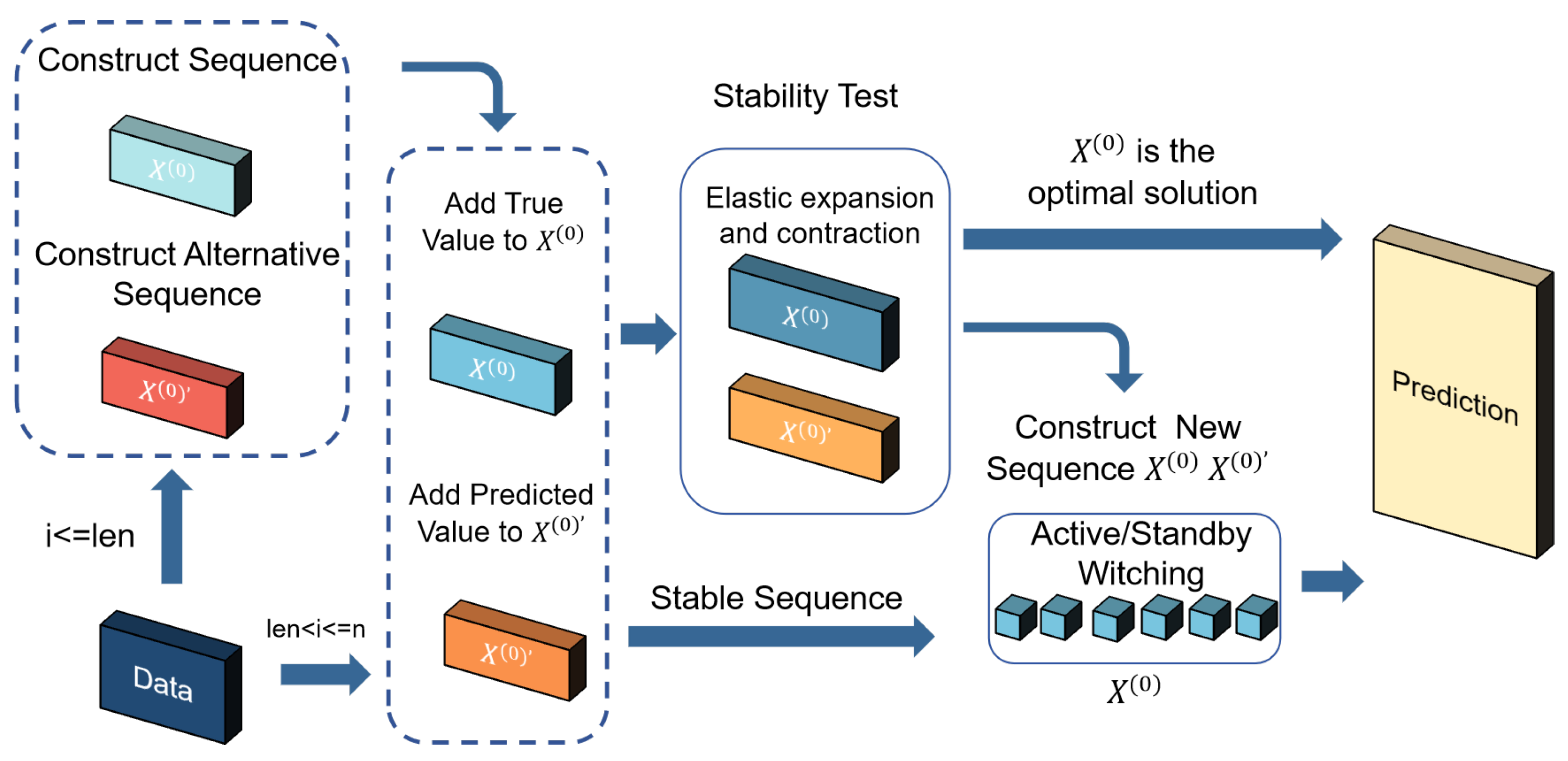
Figure 2.
Algorithmic errors in GDP.
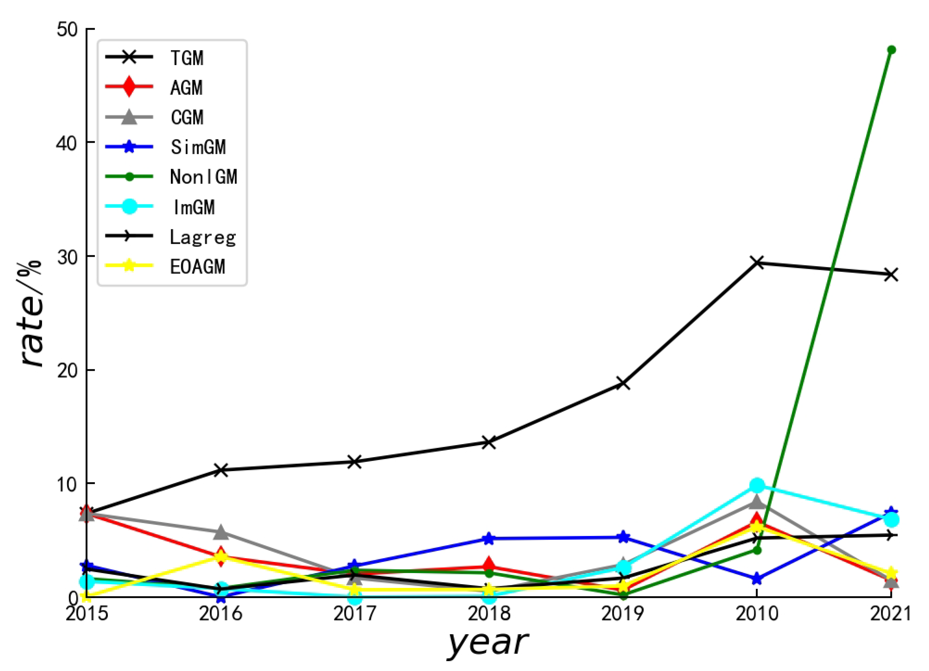
Figure 3.
(a) represents Buildings No.11.(b) represents Buildings No.12.(c) represents Buildings No.13.(d) represents Buildings No.14.(e) represents Buildings No.15.(f) represents Buildings No.16.
Figure 3.
(a) represents Buildings No.11.(b) represents Buildings No.12.(c) represents Buildings No.13.(d) represents Buildings No.14.(e) represents Buildings No.15.(f) represents Buildings No.16.
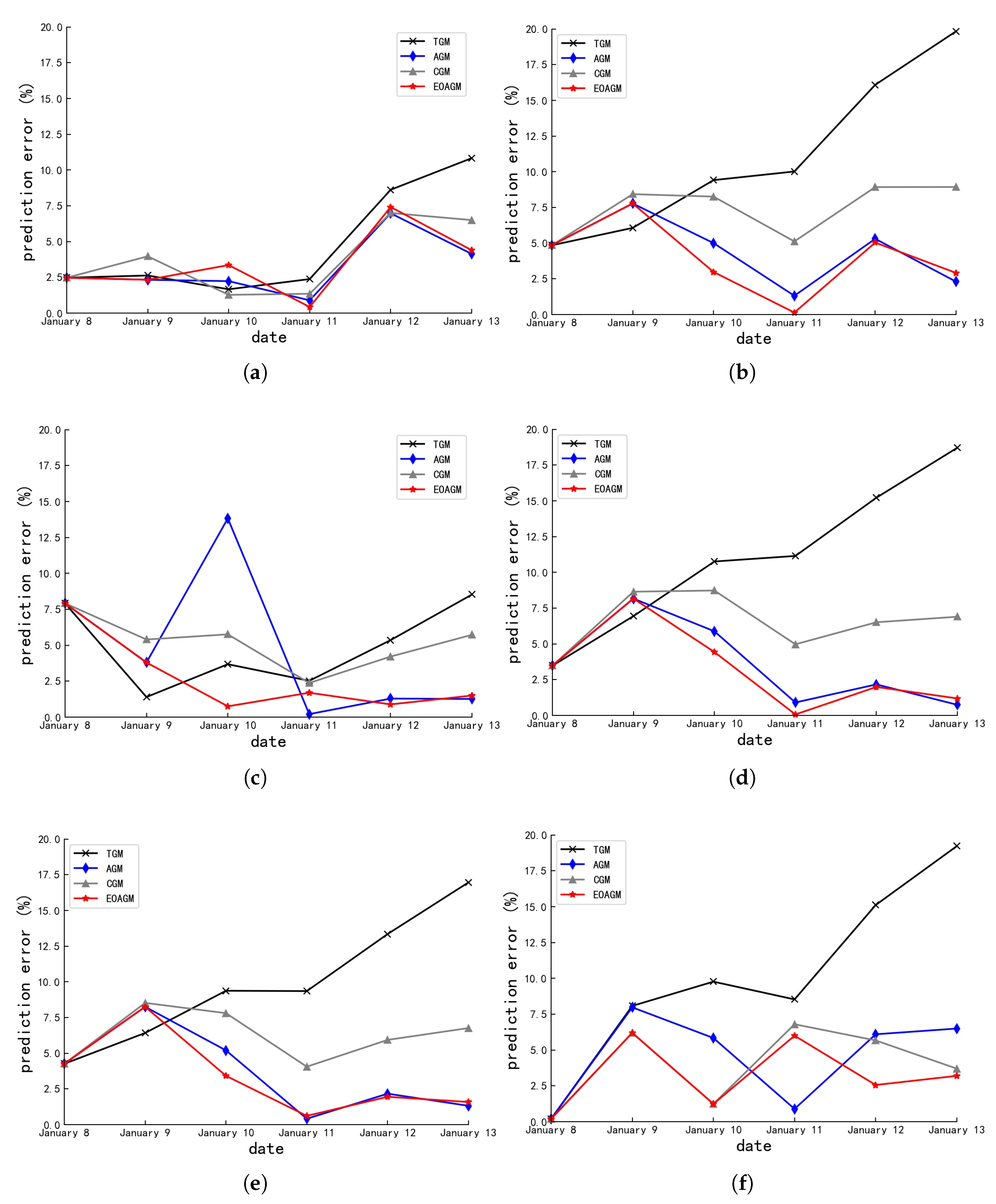

Table 1.
Raw Data of Thermal Energy Consumption.
| Date | No.11 | No.12 | No.13 | No.14 | No.15 | No.16 |
|---|---|---|---|---|---|---|
| 01-01 | 13900.29 | 3326.23 | 2536.82 | 2295.93 | 4926.74 | 17017.67 |
| 01-02 | 13556.13 | 3396.63 | 2530.54 | 2304.05 | 4882.54 | 16663.45 |
| 01-03 | 13209.10 | 3333.60 | 1914.24 | 2267.04 | 4844.14 | 16070.78 |
| 01-04 | 12385.61 | 3059.22 | 2964.36 | 2118.25 | 4544.05 | 14970.55 |
| 01-05 | 12313.99 | 3054.51 | 2338.64 | 2106.83 | 4535.83 | 14551.11 |
| 01-06 | 13223.57 | 3090.40 | 2349.92 | 2117.30 | 4585.94 | 15458.17 |
Table 2.
Comparison of algorithmic errors in GDP analysis.
| Errors | Algorithms | |||||||
|---|---|---|---|---|---|---|---|---|
| TGM | AGM | CGM | SimGM | NonlGM | ImGM | Lagreg | EOAGM | |
| 7.36 | 7.36 | 7.36 | 2.8 | 1.63 | 1.40 | 2.48 | 0.05 | |
| 11.17 | 3.56 | 5.73 | 0.02 | 0.77 | 0.749 | 0.712 | 3.56 | |
| 11.91 | 2.03 | 1.68 | 2.75 | 2.37 | 3.27e-5 | 1.95 | 0.65 | |
| 13.64 | 2.68 | 0.52 | 5.15 | 2.14 | 0.078 | 0.746 | 0.69 | |
| 18.8 | 0.62 | 2.86 | 5.26 | 0.20 | 2.60 | 1.68 | 0.98 | |
| 29.4 | 6.63 | 8.40 | 1.62 | 4.18 | 9.85 | 5.2 | 6.21 | |
| 28.4 | 1.49 | 1.48 | 7.43 | 48.2 | 6.86 | 5.46 | 2.09 | |
| 17.241 | 3.48 | 4.53 | 3.57 | 8.50 | 3.07 | 2.60 | 2.03 | |
Table 3.
Average Errors Result compare.
| Algorithms | Average Errors | |||||
|---|---|---|---|---|---|---|
| No.11 | No.12 | No.13 | No.14 | No.15 | No.16 | |
| TGM | 4.76 | 11.04 | 4.90 | 11.04 | 9.95 | 10.16 |
| AGM | 3.17 | 4.43 | 4.71 | 3.55 | 3.60 | 3.97 |
| CGM | 3.76 | 7.42 | 5.23 | 6.54 | 6.23 | 4.58 |
| EOAGM | 3.39 | 3.95 | 3.06 | 3.22 | 3.34 | 3.22 |
Table 4.
Variants on benchmark datasets.
| Dateset | Average Errors | |||
|---|---|---|---|---|
| EOAGM-A | EOAGM-O | EOAGM-E | EOAGM | |
| 4.01 | 2.43 | 3.08 | 2.03 | |
| 3.48 | 3.17 | 3.39 | 3.39 | |
| 6.85 | 4.28 | 4.16 | 3.95 | |
| 4.87 | 4.53 | 3.21 | 3.06 | |
| 6.35 | 3.55 | 3.22 | 3.22 | |
| 5.91 | 3.60 | 3.34 | 3.34 | |
| 4.27 | 3.68 | 3.54 | 3.22 | |
Disclaimer/Publisher’s Note: The statements, opinions and data contained in all publications are solely those of the individual author(s) and contributor(s) and not of MDPI and/or the editor(s). MDPI and/or the editor(s) disclaim responsibility for any injury to people or property resulting from any ideas, methods, instructions or products referred to in the content. |
© 2025 by the authors. Licensee MDPI, Basel, Switzerland. This article is an open access article distributed under the terms and conditions of the Creative Commons Attribution (CC BY) license (http://creativecommons.org/licenses/by/4.0/).
Copyright: This open access article is published under a Creative Commons CC BY 4.0 license, which permit the free download, distribution, and reuse, provided that the author and preprint are cited in any reuse.


