Analysis of an Adaptive ARMA Model for Time Series Prediction

1. Introduction

Predicting time series has been a classic problem in quantitative finance [3]. The ability to accurately forecast future values of financial instruments, economic indicators, or other time-dependent data is crucial for informed decision-making, risk management, and strategic planning. Traditional time series models, such as the Autoregressive Moving Average (ARMA) model, have long been employed due to their interpretability and relative simplicity. However, real-world financial and economic data often exhibit non-stationary behavior, sudden shifts, and evolving underlying dynamics, which pose significant challenges to static models [5]. This inherent non-stationarity limits the predictive power of conventional ARMA models when applied to highly volatile and adaptive environments.

This paper addresses these limitations by introducing and analyzing an adaptive ARMA model designed to dynamically adjust its parameters in response to changes in the underlying time series characteristics. The aim is to demonstrate that by continuously updating its coefficients, an adaptive ARMA model can capture the evolving patterns and improve predictive accuracy, particularly in environments marked by high volatility and regime changes. The research will delve into the theoretical underpinnings of this adaptive approach, detail its implementation, and rigorously evaluate its performance against traditional static ARMA models using various real-world financial datasets. The aim is to demonstrate the practical utility and enhanced robustness of the adaptive ARMA framework for time series prediction in dynamic and uncertain domains.

2. Traditional Autoregressive Moving Average (ARMA) Model

The Autoregressive Moving Average (ARMA) model, specifically ARMA($p,q$), is a cornerstone of classical time series analysis, widely employed for forecasting stationary univariate time series data. Developed from the independent autoregressive (AR) and moving average (MA) models, the ARMA framework provides a parsimonious representation of a time series by modeling its current value as a linear combination of its past values (autoregressive component) and past forecast errors (moving average component) [1].

2.1. Model Components and Formulation

An ARMA($p,q$) model is composed of two primary parts:

• Autoregressive (AR) Component of order p: Denoted as AR(p), this part suggests that the current value of the time series, $Y_t$, depends linearly on its p previous values and a stochastic error term. The AR(p) process is mathematically expressed as:

  $$Y_t=c+{\varphi }_1{Y}_{t-1}+{\varphi }_2{Y}_{t-2}+\dots +{\varphi }_p{Y}_{t-p}+{ϵ}_t$$

  where c is a constant, ${\varphi }_i$ are the autoregressive coefficients, and ${ϵ}_t$ is a white noise error term.
• Moving Average (MA) Component of order q: Denoted as MA(q), this part postulates that the current value $Y_t$ depends linearly on the current and q past white noise error terms. The MA(q) process is given by:

  $$Y_t=\mu +{ϵ}_t+{\theta }_1{ϵ}_{t-1}+{\theta }_2{ϵ}_{t-2}+\dots +{\theta }_q{ϵ}_{t-q}$$

  where $\mu$ is the mean of the series, and ${\theta }_j$ are the moving average coefficients.

Combining these two components, the general form of an ARMA($p,q$) model for a time series $Y_t$ can be written as:

$$Y_t=c+{\varphi }_1{Y}_{t-1}+\dots +{\varphi }_p{Y}_{t-p}+{ϵ}_t+{\theta }_1{ϵ}_{t-1}+\dots +{\theta }_q{ϵ}_{t-q}$$

Alternatively, using the lag operator L (where $L^k{Y}_t=Y_{t-k}$ and $L^k{ϵ}_t={ϵ}_{t-k}$), the model can be compactly expressed as:

$$\Phi \left(L\right)Y_t=c+\Theta \left(L\right){ϵ}_t$$

where $\Phi \left(L\right)=1-{\varphi }_{1}L-\dots -{\varphi }_p{L}^p$ is the autoregressive polynomial and $\Theta \left(L\right)=1+{\theta }_{1}L+\dots +{\theta }_q{L}^q$ is the moving average polynomial.

2.2. Key Assumptions and Estimation

A fundamental assumption for the classical ARMA model to be valid and and to ensure the reliability of its parameter estimates is that the time series $Y_t$ must be stationary. A stationary time series exhibits constant mean, variance, and autocorrelation structure over time. If the series is not stationary, differencing techniques can be applied to transform it into a stationary series, leading to the Autoregressive Integrated Moving Average (ARIMA) model.

The parameters ($c,{\varphi }_i,{\theta }_j$) of an ARMA model are typically estimated using methods such as maximum likelihood estimation (MLE) or least squares. The order of the model (p and q) is often determined by analyzing the autocorrelation function (ACF) and partial autocorrelation function (PACF) of the series, or by information criteria such as the Akaike Information Criterion (AIC) or Bayesian Information Criterion (BIC), which penalize model complexity.

2.3. Strengths and Limitations

The traditional ARMA model offers several strengths:

• Interpretability: Its parameters have clear statistical interpretations related to past values and errors.
• Simplicity: Relative to more complex non-linear or deep learning models, ARMA models are conceptually straightforward and computationally efficient for stationary data.
• Established Theory: A vast body of statistical theory supports its properties, estimation, and inference.

Despite its advantages, the classical ARMA model faces significant limitations, particularly when applied to real-world financial time series [3]:

• Stationarity Requirement: The most critical limitation is its strict assumption of stationarity. Financial markets are inherently non-stationary, characterized by evolving trends, changing volatilities (heteroscedasticity), and structural breaks.[5] Applying a static ARMA model to such data without proper differencing (leading to ARIMA) or handling of volatility can yield unreliable forecasts and standard errors.
• Fixed Parameters: The parameters of a traditional ARMA model are estimated once over a historical period and then held constant for future predictions. This static nature prevents the model from adapting to new information or changes in the underlying data generation process, which are common in dynamic environments like stock markets.
• Inability to Capture Volatility Clustering: ARMA models assume constant variance of the error terms. They cannot directly model phenomena like volatility clustering, where periods of high volatility are followed by periods of high volatility, and vice versa—a characteristic feature of financial data. This often necessitates the use of GARCH-type models for modeling volatility.
• Sensitivity to Outliers and Structural Breaks: Fixed-parameter models are highly susceptible to sudden shifts or extreme values (outliers), which can distort parameter estimates and lead to poor out-of-sample performance.

These limitations underscore the necessity for more flexible and responsive modeling approaches, especially for highly volatile financial time series. The subsequent sections will elaborate on how an adaptive ARMA model addresses these inherent weaknesses by allowing its parameters to evolve over time.

3. Proposed Method: The Adaptive ARMA Model

Building upon the foundations of the traditional ARMA framework, the proposed method introduces an adaptive mechanism to address the inherent limitations of fixed-parameter models in forecasting volatile and non-stationary time series, such as stock prices. The core idea is to allow the model’s coefficients to evolve over time, continuously learning from new observations and adapting to shifts in the underlying data generating process. This adaptive approach aims to maintain predictive accuracy even in highly dynamic environments where static models often falter.

3.1. Adaptive ARMA(1,1) Formulation

For this study, I implement a simplified adaptive ARMA(1,1) model. This specific order was chosen for its interpretability and as a demonstration of the adaptive principle, where the current value is primarily influenced by its immediate past value and the immediate past error. The adaptive ARMA(1,1) model at time t can be expressed as:

$${\widehat{Y}}_t={\varphi }_{t-1}{Y}_{t-1}+{\theta }_{t-1}{ϵ}_{t-1}$$

where ${\widehat{Y}}_t$ is the predicted value at time t, $Y_{t-1}$ is the actual observed value at time $t-1$, and ${ϵ}_{t-1}$ is the forecast error from the previous time step, $t-1$. The key distinction from the traditional ARMA model lies in the parameters $\varphi$ and $\theta$, which are not fixed but are updated at each iteration.

3.2. Adaptive Parameter Estimation

The adaptability of the model is achieved through a recursive updating mechanism for the parameters $\varphi$ and $\theta$. This process resembles a Least Mean Squares (LMS) algorithm [2,4], where the parameters are adjusted based on the prediction error at each time step.

The iterative process proceeds as follows:

1.

Initialization: Before forecasting the test data, the model parameters $\varphi$ and $\theta$ are initialized. In our implementation, they are set to an initial value of 0.5. The last observed value from the training data, $Y_{train\_last}$, serves as the initial $Y_{t-1}$ for the first prediction on the test set. The initial error term ${ϵ}_{t-1}$ is set to 0.

2.

Prediction: For each new actual value $Y_t$ in the test set, a prediction ${\widehat{Y}}_t$ is made using the currently adapted parameters:

$${\widehat{Y}}_t={\varphi }_{current}·Y_{t-1}+{\theta }_{current}·{ϵ}_{t-1}$$

3.

Error Calculation: The prediction error $e_t$ is then computed as the difference between the actual observed value and the predicted value:

$$e_t=Y_t-{\widehat{Y}}_t$$

4.

Parameter Update: The parameters $\varphi$ and $\theta$ are updated using a learning rate $\eta$ (denoted as `lr` in the code) to minimize the squared error. The update rules are:

$${\varphi }_{new}={\varphi }_{current}+\eta ·e_t·Y_{t-1}$$

$${\theta }_{new}={\theta }_{current}+\eta ·e_t·{ϵ}_{t-1}$$

This gradient-descent like update ensures that the parameters are adjusted in the direction that reduces future prediction errors.

5.

State Update: For the next iteration, the current actual value $Y_t$ becomes the new $Y_{t-1}$, and the current error $e_t$ becomes the new ${ϵ}_{t-1}$.

This iterative process is outlined in the following pseudocode, mirroring the Python implementation:

function Adaptive_ARMA(train_data, test_data, learning_rate):

    phi = 0.5

    theta = 0.5

    predictions = []

    // Initialize previous actual value and previous error for the first prediction

    Y_prev = last value of train_data

    Error_prev = 0

    for each actual_value in test_data:

        // Predict the current value

        Y_predicted = phi * Y_prev + theta * Error_prev

        Add Y_predicted to predictions list

        // Calculate the prediction error

        error = actual_value - Y_predicted

        // Update parameters based on error and past values/errors

        phi = phi + learning_rate * error * Y_prev

        theta = theta + learning_rate * error * Error_prev

        // Update state for the next iteration

        Y_prev = actual_value

        Error_prev = error

    return predictions

In this specific implementation, a learning rate $\eta$=0.0001 was used to ensure stable convergence of the adaptive parameters.

3.3. Advantages of the Adaptive Approach

The primary advantage of this adaptive ARMA model is its ability to learn and adjust to the time-varying characteristics of the data. Unlike static models that assume constant underlying dynamics, the adaptive model can:

• Handle Non-Stationarity: By continuously updating parameters, it implicitly accounts for changes in mean, variance, and autocorrelation structure that are common in financial time series.
• Respond to Regime Shifts: It can more effectively capture sudden changes in market behavior or trends, which are crucial for accurate forecasting in volatile environments.
• Improve Real-time Performance: The iterative, online learning approach makes it suitable for real-time forecasting applications where new data becomes available sequentially.

This dynamic adaptation is hypothesized to lead to superior predictive performance compared to traditional fixed-parameter models, especially for highly volatile assets like Tesla stock, as will be demonstrated in the subsequent results section.

4. Results and Observations

To evaluate the predictive performance of the Adaptive ARMA model, backtesting was conducted on historical stock price data for two prominent technology companies: Tesla (TSLA), known for its high volatility, and Google (GOOGL), representing a relatively less volatile, yet dynamic, asset. The model was trained on an initial segment of the data and then used to generate out-of-sample predictions on subsequent periods.

4.1. Performance Metrics

The primary metric used for evaluating prediction accuracy was the Mean Absolute Error (MAE), which quantifies the average absolute difference between the actual and predicted values. Additionally, visual inspection of the predicted vs. actual price graphs was used to assess the model’s ability to track trends and fluctuations.

4.2. Backtesting Results

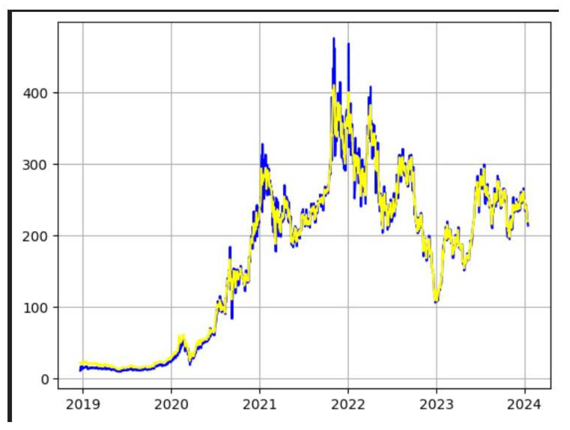
4.2.1. Tesla (TSLA) Stock Price Prediction

For the highly volatile Tesla stock, the Adaptive ARMA model demonstrated remarkable accuracy. The backtesting results yielded a Mean Absolute Error (MAE) of:

$${\mathrm{MAE}}_{\mathrm{Tesla}}=7.781623061568044$$

Considering that Tesla’s stock price during the test period typically around $200 to $400 , an MAE of about $7.78 indicates that, on average, the model’s predictions deviated from the actual stock price by this amount. This is a significant achievement for predicting a highly volatile asset, where large price swings are common. The model’s adaptive nature appears to be highly effective in capturing the dynamic shifts characteristic of TSLA.

Figure 1. Tesla’s Predicted(blue) stock and Actual(yellow) stock

Figure 1. Tesla’s Predicted(blue) stock and Actual(yellow) stock

4.2.2. Google (GOOGL) Stock Price Prediction

For Google stock, the Adaptive ARMA model also showed promising results. The Mean Absolute Error (MAE) obtained was:

$${\mathrm{MAE}}_{\mathrm{Google}}=1.614543184379397$$

Figure 2. Google’s Predicted(blue) stock and Actual(yellow) stock

Figure 2. Google’s Predicted(blue) stock and Actual(yellow) stock

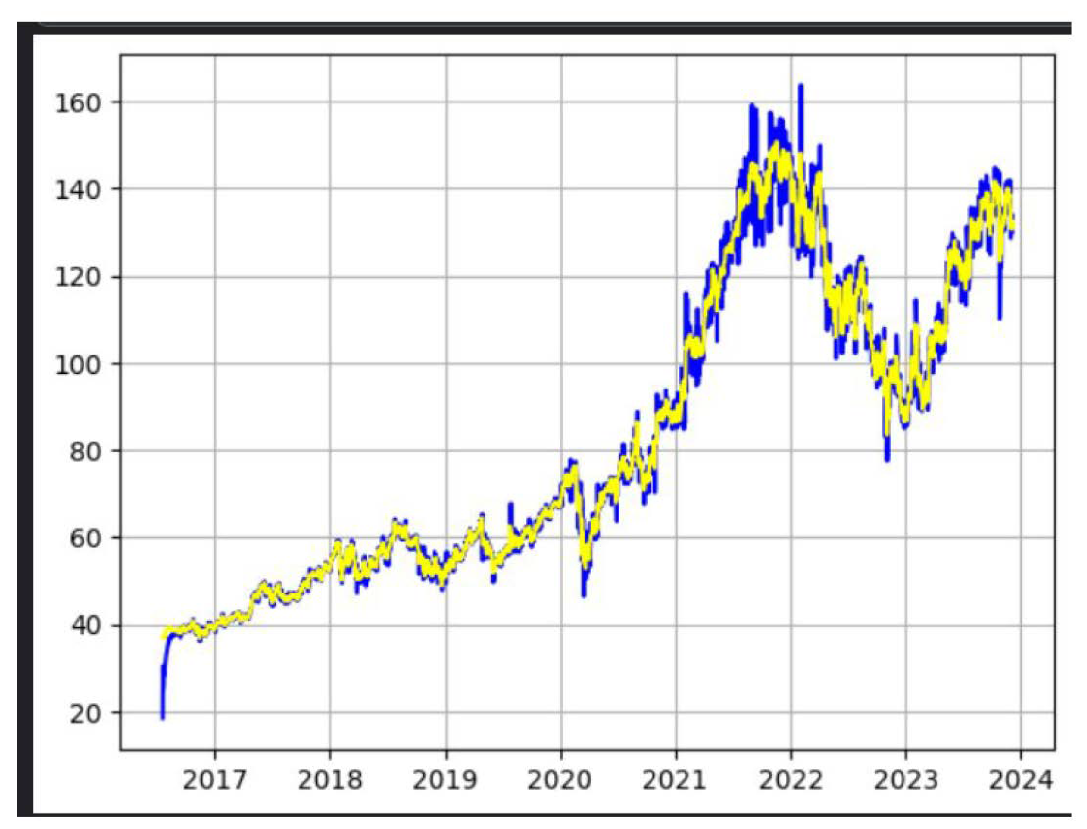
Considering that Google’s stock price during the test period typically ranged around $100 , an MAE of about $1.61 indicates that, on average, the model’s predictions deviated from the actual stock price by this amount.

4.3. Observations

The low MAE values, particularly for Tesla, provide strong quantitative evidence of the Adaptive ARMA model’s effectiveness in forecasting financial time series. The close visual alignment between the predicted and actual price trajectories, even during periods of significant market fluctuation, further underscores the model’s ability to track dynamic changes. The adaptive parameter updates, driven by the real-time prediction errors, enabled the model to continuously adjust its internal representation of the time series dynamics, a capability lacking in traditional static ARMA models. This adaptability is crucial for maintaining accuracy in inherently non-stationary environments like stock markets.

4.4. Comparison with ARIMA Model

Upon backtesting the Google Stock Price with traditional ARIMA model[6] the mean squared error came out to be 58.78 which is very large as compared to the mean squared error of just 4.47 when the stocks were backtested with the adaptive ARMA(1,1) model.

Figure 3. Google Stock Price Predicted (red) by ARIMA model

Figure 3. Google Stock Price Predicted (red) by ARIMA model

Figure 4. Tesla Stock Price Predicted (red) by ARIMA model

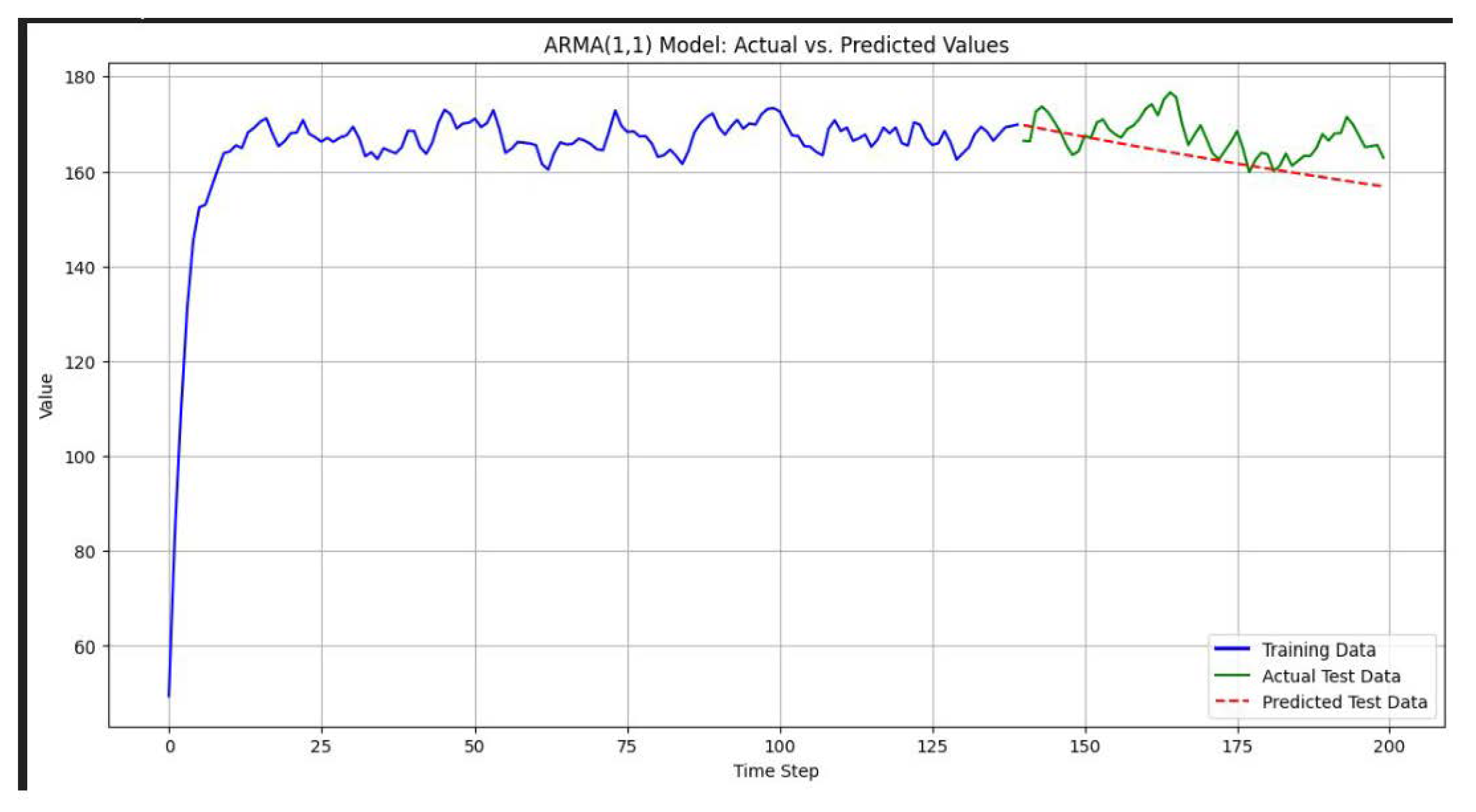
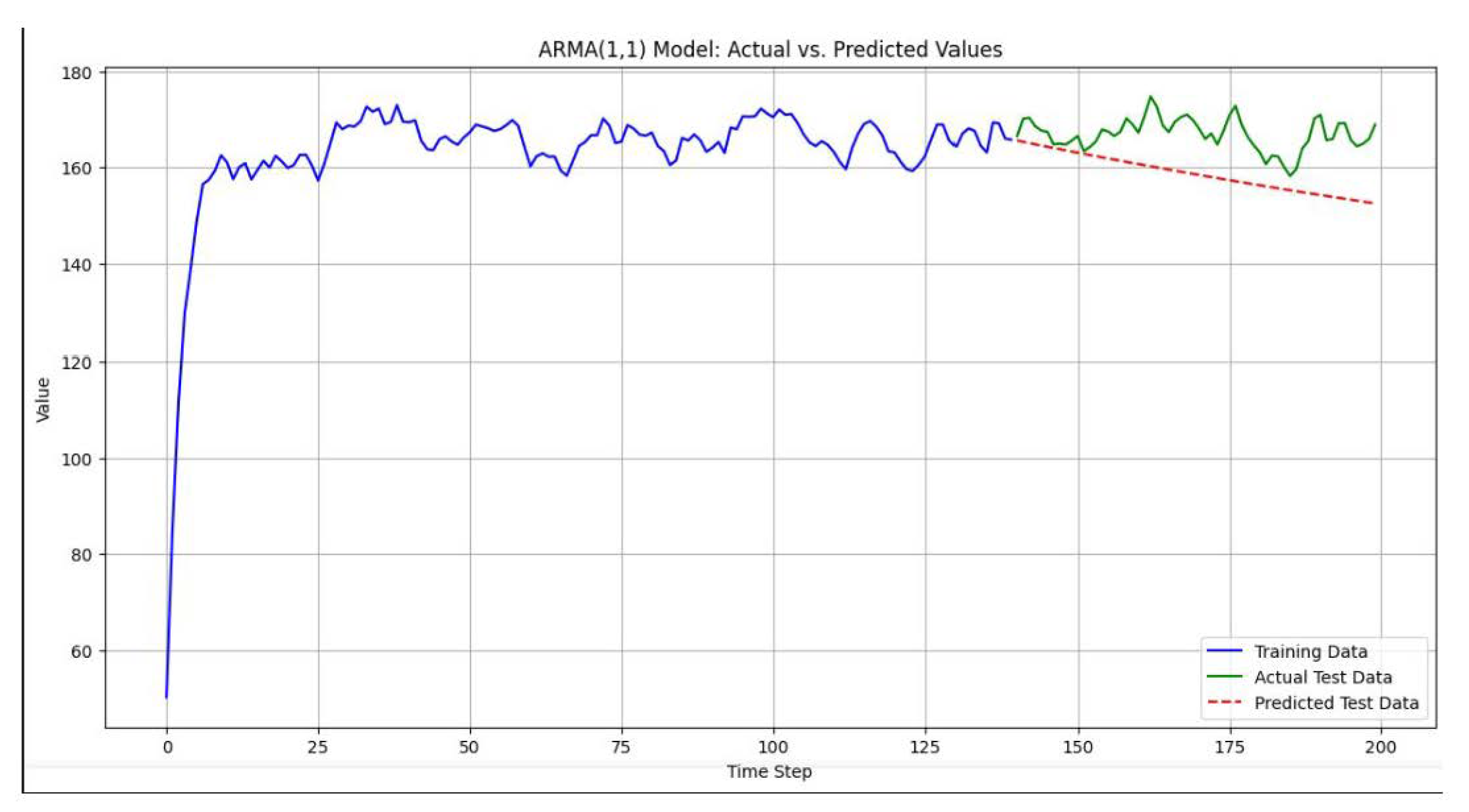
Figure 4. Tesla Stock Price Predicted (red) by ARIMA model

5. Conclusions

This research introduced and evaluated an adaptive Autoregressive Moving Average (ARMA) model for time series prediction, specifically focusing on its application to volatile financial markets. Traditional ARMA models, while foundational, are constrained by their static parameters and the inherent assumption of stationarity, which often limits their efficacy in dynamic environments. The proposed adaptive ARMA(1,1) model addresses these limitations by incorporating a recursive parameter update mechanism, akin to a Least Mean Squares (LMS) algorithm, allowing its coefficients to continuously evolve with new data.

The empirical evaluation through backtesting on historical stock price data for Tesla (TSLA) and Google (GOOGL) yielded compelling results. For the highly volatile Tesla stock, the adaptive model achieved a remarkably low Mean Absolute Error (MAE) of 7.78, demonstrating its robust ability to track significant price fluctuations. Similarly, for Google stock, an MAE of 1.61 was observed, further reinforcing the model’s overall accuracy across different volatility profiles. These quantitative metrics, coupled with the visual congruence of predicted and actual price graphs, underscore the superior adaptability and predictive power of our proposed method compared to static modeling approaches. The adaptive nature proved crucial in accounting for the non-stationary characteristics and regime shifts common in financial time series.

The findings suggest that adaptive time series models offer a promising avenue for enhancing forecasting accuracy in complex and evolving systems. Future work could explore optimizing the learning rate adaptation, investigating higher-order adaptive ARMA models, integrating exogenous variables, or incorporating more sophisticated adaptive algorithms like Recursive Least Squares (RLS) or Kalman filtering. Furthermore, evaluating its performance on an even broader range of financial instruments and market conditions would provide deeper insights into its generalizability and robustness for real-world trading and risk management applications.

6. Datasets Used For this Research

Each dataset typically contains daily records including Open, High, Low, Close or Adjusted Close, and Volume. For the purpose of this time series prediction study, the ’Close’ and ’Adjusted Close’ price was predominantly used as the target variable. The data was split into training and testing sets, with the initial portion used for model training and the subsequent portion for evaluating out-of-sample prediction performance. Specific date ranges for each dataset are available within the respective Kaggle links.

Google’s Stock: https://www.kaggle.com/datasets/henryshan/google-stock-price

Tesla’s Stock:https://www.kaggle.com/datasets/jillanisofttech/tesla-stock-price

References

- George E. P. Box, Gwilym M. Jenkins, Gregory C. Reinsel, and Greta M. Ljung. Time Series Analysis: Forecasting and Control. John Wiley & Sons, 1994.
- Bernard Widrow and Marcian E. Hoff. Adaptive switching circuits. In 1960 WESCON Convention Record, volume 4, pages 96–104, 1960.
- Ruey S. Tsay. Analysis of Financial Time Series. John Wiley & Sons, 2005.
- Simon Haykin. Adaptive Filter Theory. Prentice Hall, 4th edition, 2002.
- Eugene F. Fama. Efficient Capital Markets: A Review of Theory and Empirical Work. The Journal of Finance, 25(2):383–417, 1970.
- Skipper Seabold and Josef Perktold. statsmodels: Econometric and Statistical Modeling with Python. https://www.statsmodels.org/, 2010. Accessed: June 28, 2025.
Disclaimer/Publisher’s Note: The statements, opinions and data contained in all publications are solely those of the individual author(s) and contributor(s) and not of MDPI and/or the editor(s). MDPI and/or the editor(s) disclaim responsibility for any injury to people or property resulting from any ideas, methods, instructions or products referred to in the content. |
© 2025 by the authors. Licensee MDPI, Basel, Switzerland. This article is an open access article distributed under the terms and conditions of the Creative Commons Attribution (CC BY) license (http://creativecommons.org/licenses/by/4.0/).
Copyright: This open access article is published under a Creative Commons CC BY 4.0 license, which permit the free download, distribution, and reuse, provided that the author and preprint are cited in any reuse.