Submitted:
22 April 2025
Posted:
23 April 2025
You are already at the latest version
Abstract
The most straightforward approach to installing the drone components is to use metal screws, which is why the metal brasses were put into printed drone parts using a heat-stuck procedure. Six printing combinations were used for printing the drone arm. The infill density and raster line were set to 35% and 0.3 mm, respectively. Other printing factors varied, including the wall line contour and thickness, as well as the number of top and bottom layers. The main objective was to assess the quality of the joint between plastic and metal inserts following natural and artificial aging. The pull-out force was measured using a standard pull-off tester and tensile test device after 2 hours of brass insertion, 15 days and 1 year of aging at room temperature, 28 days in a climate chamber without IC and UV light, 44 days in a climate chamber with IC and UV light, 2 minutes in liquid nitrogen, and a frost resistance test. FTIR, colorimetric and wettability analyses were used for monitoring of deterioration. Based on the experimental results the optimal 3D printing combination was selected. The samples for flexural strength were also produced using the previously mentioned printing parameters. The evaluation of stresses generated in the drone arm during exploitation was modeled. The printed arm was cantilevered and the axial force was continually applied at its end until failure. Experimental data were compared with the simulation. The results revealed that the functional joint between metal brass and plastic remained intact after aging and that PLA is a suitable material for drone arms applications with a maximum loading capability of 9.24 kg.
Keywords:
Additive manufacturing
; Aging
; Heat stuck process
; FTIR
; Industry 4.0
; Analytical modeling
; AEC
Highlights
- The success of maintaining joint functionality between PLA and brass inserts after various aging protocols.
- PLA's suitability for drone applications even at lower infill densities.
- A note about future work involving higher infill densities and more combinations of parameters.
1. Introduction
Additive manufacturing (AM) is a well-accepted and widely utilized method for producing diverse components, prototypes, and parts, as well as customized tools and accessories through a layer-by-layer construction process. AM is constantly evolving to expand and find its place in as many possible different industrial sectors including AEC (Architecture-Engineering-Construction) [1]. One of the most significant advantages of this method is the relatively fast production of geometrically complex parts which is even more actual if serial production is not required [2].
Metal threads are utilized for joining materials in a variety of industries, including metal structures, shipbuilding, automobiles, electronics, aircraft, and defense. Its application is increasing, especially when rapid construction and disassembly of pieces is required [3]. There is an absence of thorough studies analyzing the quality of metal inserts used in AM-produced plastic parts. Such joints are essential because their quality influences the final product's intended purpose. This is particularly valid when it comes to joining larger products. Today, the industry has simply embraced metal and plastic joints during the assembly process, which demands rapid connection of smaller pieces [4]. The maximal pull-out force is a widely accepted criterion for quantifying the quality of the joint between metal insert and plastic. During testing, the force required to pull the threaded insert out of the plastic is continually measured. Generally, this is still not a standardized method even though this force can be measured on standard pull-out or tensile test devices. This means that researchers do not always employ the same preset parameters throughout testing, such as loading speed and sample dimensions [5].
Several methods (insert molding, thermal, cold and ultrasonic insertion) are available for joining thermoplastic material with metal insert [6,7]. Amancio et. al. [8] have analyzed three techniques for joining polymers and their composites: mechanical fastening (screws or rivets), adhesive bonding, and welding (melting the materials to form a joint). Each of these techniques has its advantages and disadvantages. Namely, mechanical joining has certain difficulties due to the different physical and chemical properties of metals and polymers (thermal expansion, surface energy, and mechanical strength). Besides the characteristics of the materials used for joining have a huge impact on the durability and design of final products. Metal inserts (or threatened inserts) offer better qualities than printed parts in which they are embedded, particularly those related to stress-strain relationships.
Heat stuck is a commonly used technique for joining metal and printed plastic. The main advantage of this method is that the joining process does not require drilling that additionally affects the mechanical properties of the plastic parts obtained by AM [3]. During embedding the softened plastic adheres to the outer surface of the insert. This process can be realized by different procedures [9]. The strength of the joint is greatly influenced by the joining technology, the geometry of the insert and preset printing parameters, for example specified number of top and bottom layers and wall line contours [10]. The strongest connections are made by directly sinking metal threaded inserts into the plastic [5]. Recently Fürst et al. [11] have presented an innovative procedure, in which heat input is delivered via outer thread flanks during application. This method can increase the overall strength of the joint compared to the standard heat stuck procedure. Miklavec et. al. [12] have used different forms of metal inserts to improve the mechanical characteristics of the hybrid joint. Results have confirmed that the design of metal inserts, especially its outside surface is a very important parameter for ensuring better polymer bonding to the metal which consequently leads to the increase of its strength and corrosion resistance. Furthermore, the folds on the outside of the metal inserts have a direct impact on pullout resistance and torque [13]. An investigation into the possibilities of enhancing the stiffness and mechanical strength of the composite carbon fiber reinforced plastic is another example of how the geometry and form of the metal insert impact the joint [14]. An additional bed patterns were added to the metal sheet of the insert. This technology significantly increased the performance of composite products, particularly their load-bearing capability. Thereby composite components can be linked with other materials more readily and robustly. The influence of printing parameters on the quality of the joint between the insert and plastic was reported in the study by Kastner et al. [15]. It was found that infill density has a significant effect on the joint strength. A direct relation between infill density and the pulling force was registered. Optimal printing preset was also reported. Recommended infill density, wall thickness, layer height and print temperature were set to 70%, 1.2 mm, 0.2 mm, and 225°C. When it comes to sandwich panels, the performance of inserts subjected to pulling forces was also investigated. For example, Seeman et al. employed numerical models to predict pull-out strength [16], whereas Stefan et al. experimentally investigated the mechanical properties of panels with inserted metal joints under various loading conditions [17].
Degradation is commonly seen as the deleterious distortion of the material: surface appearance (color change), chemical structure, or physical properties. In the polymer case, degradation occurs as a result of macromolecule chemical cleavage. Various mechanisms (photo-oxidative, thermo-oxidative, ozone-induced, mechanochemical, hydrolytic, freeze-thaw and biodegradation) which can act separately or simultaneously are causing the polymer chain scission. Besides, polymer aging is commonly seen as the gradual degradation of material over time caused by environmental factors such as heat, moisture, oxygen exposure, light (UV radiation) or mechanical stress [18-20]. Accelerated aging refers to any artificial procedure that increases one or more variables affecting the material's natural decay. The primary goal is to simulate the long-term effects of environmental conditions in a shorter time frame. Orellana-Barrasa et al. [21] have aged PLA in a temperature range from 20 to 80°C. It was found that PLA can be safely aged without degrading at 39°C. Vorkapić et al. [22] have studied the impact of temperature aging at 57°C on the tensile properties of PLA printed samples. It was found that with aging the mechanical properties are decreasing. This is more pronounced for samples printed with higher layer height. Products with 0/90[°] orientation were mostly brittle while those printed using -45/45[°] orientation withstood the highest deformations before failure. The impact of UV radiation on PLA samples can be found for example in references [23-25]. References [25,26] described PLA weathering tests utilizing the methodology that included two (humidity and temperature) and three (humidity, temperature, and UV) aging agents. The main finding was that mechanical properties were lower for samples aged at maximal relative humidity content.
Standards ISO 2578, ISO 176, and ASTM D1203 are used for determining heat stability and formulating long-term predictions about polymers. Heat distortion of polymers is described in ASTM D648. The problem is that most standards for assessing polymer weathering degradation are limited to a particular degrading agent, such as ASTM D1435, D1499, D2565, D4329, or D4364. The lack of corresponding ISO or ASTM Cyclic Laboratory Conditions aging standards which include all aging mechanisms is evident. It is important to state that the existing long-term polymer performance assessment is limited and has to be taken with caution, especially when assessing factors are apparent. In such situations, its validity is questionable [27]. As a result, many aging processes were used in this work, including a novel full cycling method that included four aging parameters (relative humidity, temperature, UV, and IC radiation) at the same time. Furthermore, the effect of artificial aging on the joint between inserts and plastic has not been recorded in literature.
2. Materials and Methods
2.1. Drone Design
The drone arm design is important for both mechanical and dynamic loading. The arm cross-section is important from the aspect of load-bearing capacity (strength) and satisfying aerodynamic properties [28]. They usually have a circular or rectangular cross-section, but can also be triangular or T-shaped. In general, the rectangular cross-section is the strongest and provides the required mechanical performance, while the circular cross-section is the most aerodynamically efficient [29]. The goal is to design a drone that will have its purpose according to the defined payload [30]. Guidelines and suggestions for the maintenance of an unmanned aerial vehicle (UAV) are given in the paper [29]. In the same paper the mechanical stress on the arm drone was also analyzed using the finite element method and the weak points in the design of the complete UAV were identified. Tripolitsiotis et al. [31] analyzes the realization of the drone frame modular design. The concept of "modularity" is extremely important in the development of drones, especially when it comes to adaptability to specific missions (for terrain mapping, natural disasters, and military purposes). Also, modularity promotes ease of maintenance and rapid interchangeability, the possibility of modifications and the application of new innovative solutions (when using a new material/composite or during the design process) in the realization of drone elements.
The drone's adaptability must match mission objectives, including payload, thrust-to-weight ratio, efficiency, flight time, and maximum speed. Interchangeability of parts means that a broken or obsolete component can be replaced, considerably lowering costs and repair times. Spare parts manufacture is required, particularly for commercial or mission-specific drones [32]. Motors with propellers are mounted to the drone arms. This allows the drone to be raised and lowered while maintaining controllable thrust. Additional elements can be attached to the arms depending on the intended use of the drone. For this reason, the arms must be strong enough to withstand the impact forces during landing or the torque of the motors and propellers [33]. The shape and lift of the shoulder largely affects aerodynamics and flight efficiency. The airflow must be able to move freely around the engine and propeller. In this scenario, shoulder length and distance are critical to avoiding propeller collisions [34]. The principle of attaching drone arm elements is described in detail in the Prado`s dissertation [35] using the example of a quadcopter. The quadcopter was manufactured using additive technology. In a detailed work, the author established the drone layout and examined the usage of various materials, engines, and frame configurations, resulting in the creation of an unmanned aerial vehicle with a lightweight frame with good mechanical properties. In the quadcopters, the X configuration, this design improves stability, but aerodynamic performance is a problem [36], as the arms are located between the top and bottom plates, which restricts and complicates the placement of other vital elements of the drone in many cases.
Based on the aforementioned sources, a similar analysis of attaching the arm drone with other frame elements was conducted in this paper. As can be seen in Figure 1, threaded inserts are pressed into the drone arms using the heat-stacking technology described previously. The technique of arms connecting to the top and bottom plates is done by pressing the protrusions on the arms into specially designed holes on the plate.
The links between the plates, the arms and the legs are solid and compact. Similar modular solutions have been described many times in the literature [30,37-39]. The appearance of the central part of the drone frame is also new. The study [40] includes an inner cylinder between the upper and lower plates that can accommodate four, six, or eight arms. The connection of the cylinder to the arms is realized by threaded inserts. Threaded inserts drowned in plastic have also been shown. In the event of minor impacts or collisions, the connection of the shoulder to the plates allows the impact to be absorbed and other components to be protected. All this extends the life of the drone and reduces repair costs. The connection via threaded inserts enables the arm to be replaced quickly in the event of damage. The position of the brass inserts in the drone arm is shown in Figure 2.
2.2. Employed Materials and Methodology
A commercial white PLA thermoplastic filament with a diameter of 1.75 mm was used in this study. According to its data sheet (available at the Creality [41]) it was concluded that the mechanical properties (tensile, bending and impact strength) comply with the preset project requirements for the drone arm's intended use. Besides, this material is derived from renewable sources and belongs to the group of biodegradable materials [42,43]. It is also cheap and extremely available on the market.
Before printing, the 3D CAD technical drawing is first converted to STL format, which is then converted to G-code because it is the only standardized native file that printing device software can recognize and use. All samples were printed on a Creality Ender-6 device using an extruder with a nozzle diameter of 0.4 mm. The preset printing parameters are given in Table 1. The other parameters: print temperature 210°C, bed temperature 60°C, infill speed 60 mm/s, infill density 35%, raster line 0.3, infill line direction -45°/+45°, infill pattern zig-zag and travel speed 80 mm/s were constant.
The metal brass inserts [44] were emended into the samples using the heat stuck procedure. The metal insert was initially placed vertically on the surface of the sample. A soldering iron which was previously heated to the temperature of 230°C was placed inside the metal brass and the insertion process was carried out. Once the insert is aligned with the sample, the soldering iron is removed. Special care was taken to ensure that during insertion a minimal force is applied as recommended in references [7,45-46].
During this process, the heat spread through the brass was used to liquefy the plastic within a close narrow zone commonly called melting (Figure 3a). The plastic flows around the brass inserts are registered in this zone.
The soldering iron probe must not overheat the insert, as this will cause the thermoplastic material to burn and the hole to expand, resulting in a loose connection [47]. Furthermore, the dimension of the central hole has a direct impact on the adhesion bond between the metal insert and the thermoplastic polymer. It is consequently necessary to precisely determine its diameter. If it exceeds the outer diameter of the metal insert, a poor connection will be produced during the heat stack process (Figure 3b). In the opposite circumstance, more impact force will be applied, and excess plastic will be extruded. The hole guarantees a secure connection only after the metal insert is fully embedded in the plastic [48-50]. Preset printing parameter combinations are provided in Table 1.
During printing, dimensional deviations can occur as a consequence of material shrinkage, layer adhesion or inadequate printer calibration. In this case, inadequate printer calibration factor can be excluded since regular maintenance (checking the filament storage, printer alignment and nozzle cleaning) was applied. The fact that no warping impact was identified on printed samples suggests that the second-factor layer adhesion is satisfactory and may be ignored. This means that any minor dimensional differences are mostly caused by the PLA filament contracting while cooling. That is why the central hole was somewhat larger than the brass insert, as shown in Figure 4.
Samples with inserted brass were naturally and artificially aged. After aging the quality of the joint between the plastic and metal inserts was evaluated. The pull-out force was determined. Measurements were conducted on the laboratory CONTROLS pull-off tester and the Shimadzu compact table-top universal tensile tester. Both devices have a capacity of 5 kN. Initially, a specialized adaptor tool was built. It was utilized as a sample holder for the tensile tests. The tool is composed of aluminum and created using traditional machining techniques (lathe, milling machine). It is made up of two components as illustrated in Figure 5.
At the onset of the test, the sample is placed in the holder. The upper component of the holder is positioned above the sample to fix it. Then a threaded rod is screwed onto a metal insert. A threaded rod is then fastened to the lower section of the tool. The higher jaws fasten the upper threaded rod screw, and the lower jaws lock the lower threaded rod. This connection ensures that the sample is positioned correctly in the tensile device during testing. The joint's load capacity is defined as the greatest force that the sample can withstand before the metal insert detaches (pulls out) or breaks/tears.
Samples were first analyzed two hours after brass implantation. The test designation code is SP. The natural procedure (NP) assumes that samples were examined after three months and one year of maturing at room temperature. Several test panels were constructed (Figure 6a). The first panel raw was created by combining three samples from the first printing combination. The next raw represents the second printing combination. This technique was repeated until the sixth panel raw was created. Each sample was isolated from all sides except one using a Styrofoam and a rubber joint.
The initial artificial protocol (AP-I) consisted of 22 cycles. Samples were aged during 44 days (31.01. – 15.03.2024) in the Binder KBWF 240 climatic chamber equipped with 2 illumination cassettes with IC and UV light. One cycle lasted for two days. During the first day, the winter weathering conditions were simulated. Temperature and relative humidity were kept at 5°C and 80%. Throughout the second day, the summer weathering conditions were reproduced. Temperature and relative humidity were kept at 400°C and 25%. The panel was removed from the chamber after 14, 29, 37, and 44 days for about 30 minutes. During this time, FTIR analysis, colorimetry, and wettability tests on the material's surface were performed. After that, the test panels were assembled again and returned to the chamber. The contact angle measurement was performed using the Surface Energy Evaluation System, Advex Instruments, Brno, Czech Republic, with demineralized water as the measuring fluid. FTIR analysis was conducted using the Alpha (BRUKER Optics, Germany) FTIR instrument with a DRIFT (Diffuse Reflectance) attachment for non-contact measurements, in the wavenumber range of 400 to 4000 cm-1 and a resolution of 4 cm-1. The FTIR spectrum for each measurement position is an averaged spectrum of 24 scans. The obtained FTIR spectra were then analyzed using the OPUS software (BRUKER, Germany). The spectrograph software version 1.12.16.1 was used for plotting the FTIR raw data and finding peaks values [50].
The second artificial aging protocol (AP–II) assumes the aging in the climate chamber without IC and UV lamp for 28 days. A test panel was firstly kept for 8 h in the air which relative humidity temperature and velocity were respectively 80%, 40°C and 1m/s (Figure 6b). After that, the panel was taken out and left in the desiccator for the next 16 hours at a temperature of 25°C. One cycle has lasted 24 hours. Sample mass during the first 8 h of each cycle was recorded. Temperature, humidity and velocity were regulated inside the chamber with the accuracy of ± 0.2°C, 0.2% and 0.1 m/s. Mass was recorded with an accuracy of 0.01 g.
The following three artificial aging protocols (AP-III, AP-IV, and AP-V) assess the long-term durability of materials through freeze-thaw resistance tests conducted under severe and extreme conditions. Two durability tests were performed under severe conditions. The first test (AP-III) was based on the EN 772-22:2018 standard. The test panel was placed in a freeze-thaw slab tester (TESTING, Germany), where each cycle consisted of a freezing and thawing phase. The air temperature, measured (40 ± 10) mm from the exposed surface, was gradually reduced from 20°C to −15°C, over 30 minutes. The panel was then maintained at −15°C for 100 minutes. Warm air was introduced to facilitate thawing, with this phase limited to 20 minutes. Upon completion of 100 freeze-thaw cycles, the panel was disassembled, and each sample was carefully examined for defects such as surface cracks, through-cracks, scaling, chipping, or peeling.
In the second severe test (AP-IV), the panel was placed in the same slab tester, pre-set to −20°C, and held at this temperature for 4 hours. It was then removed and left at ambient conditions (room temperature) for another 4 hours. The test lasted 40 days (120 cycles). The durability test under extreme conditions (AP-V) involved immersing individual samples in the liquid nitrogen container for 2 minutes.
Standard dog bone samples were printed for each printer combination. The test was carried out by the EN ISO 572-2 standard. The test speed was set to 50 mm/min. The Shimadzu compact table-top universal tensile tester was used. Three drone arms, whose dimensional characteristics are given in Figure 7, were fabricated using printer combination IV. The printed arms were left on a desk at room temperature for one year (NP-I protocol). After that, they were placed in a special tool designed to hold the arm in a cantilevered position. An axial force was continuously applied at the arm’s end until failure. The Instron 1122 universal test device, equipped with a TRC Pro acquisition system and a maximum load capacity of 5 kN, was used. The speed was set to 50 mm/min.
In addition to the experimental investigation of the drone arm, a numerical analysis was conducted to compare its behavior, determine the overall stress state, and assess the onset of material plasticization. The geometric model of the drone leg was designed to fully correspond to the physical model, with a length of 218.5 mm and a maximum width of 40 mm. The thickness of the drone leg is 10 mm. The input values for: elastic modulus, Poisson’s ratio, and specific weight were respectively 1605 N/mm², 0.3 and 1240 kg/m³. The value of the elastic module was obtained from the tensile test results conducted in this study for printing combination IV. A concentrated load of 120 N, acting orthogonally to the mid-plane of the drone arm, was used. This value represents the maximum force that the printed arm withstood during testing performed in this study. The static analysis of the drone arm was performed using the Finite Element Method (FEM) in the AxisVM software.
3. Results and discussion
The averaged pull-out force results are summarized in Table 2. Figure 8 illustrates the decrease in pull-out force observed after both natural and artificial aging compared to the initial measurements taken before any aging conditions (SP). Both natural and artificial aging significantly decreased the pull-out force. The highest decline is observed in the case of AP-I, which was expected given that this aging protocol comprised temperature cycling, humidity exposure, dry/wet cycle circumstances, combined load, and environmental exposure to UV and IC radiation. Notably, a similar drop in force is observed with AP-II.
The obtained results suggest that the degradation effects caused by freeze-thaw protocols under severe conditions, namely AP-III and AP-IV, are comparable. Additinally, the extreme freeze technique resulted in a stronger pull-out force than any of the severe freeze-thaw methods. However, this "increasing" effect on mechanical properties after extreme exposure was not unexpected, as it was also noted and discussed in our previous study involving PETG samples [51].
As can be seen in Fig. 8. the pull-out force is in direct correlation with the set printing parameters. As previously stated, its value has consistently increased from samples IV to XII. This pattern was observed for all aging treatments. The nozzle movement during sample realization was visualized using the Ulitmaker Cura software. The output images for samples IV – VI are given in Figure 9. Samples VI and XII are "stronger" around the hole than samples printed with two or three wall line contours.
The morphology of the tested samples after the pull-out test for NP-II, AP-III and AP-V is illustrated in Figure 10. Samples aged under protocol NP-I, AP-I and AP-II have a similar appearance. As can be seen in Figure 11, AP-IV was the only set where a distinct morphology pattern was observed.
Furthermore, each pull-out metal insert was covered in plastic in this instance as well. In addition, the thickness of the plastic layer around the implant increased from samples IV to VI and from samples X to XII. This is valid proof that the heat stack insertion method was successful. Also, since other printing parameters, such as infill density and infill line direction, were constant in the study it is obvious that the number of wall line contours is responsible for the observed pull-of-force trend. This was also in line with the findings reported in reference [52].
The quantification of the long-term degradation caused by aging was given for AP-I as an example. FTIR measurements are summarized in Figure 12, Figure 13, Figure 14 and Figure 15. To study the degradation exhibited in the provided spectroscopic data over a 44-day period (31.01.2024-15.03.2024), multiple critical observations are examined: absorption trends and peak shifts. The absorbance values across the different dates generally show consistent behavior, with some peaks and troughs reflecting chemical changes over time. Certain peaks observed around specific wavenumbers appear to shift or change intensity over time.
The absorbance spectrum obtained on the first day of the investigation (31.01.2024) presents a characteristic baseline with peaks, indicating the initial state of the material being studied. Minor changes are observed after 14 days (13.02.2024) compared to the baseline, suggesting an initial phase of degradation or stabilization. At 29 days (28.02.2024) the spectrum appears more pronounced in certain absorbance peaks, indicating further degradation or alterations. New peaks are emerging, suggesting changes in chemical bonds. At 37 days (8.03.2024) the absorbance likely continues to increase or shift, hinting at ongoing degradation. Specific peaks show significant intensity changes, possibly indicating compound breakdown. At 44 days (15.03.2024) the spectral features are mostly pronounced, showing the final extent of degradation.
Broad peak (3984–3850 nm range) present initially (31.01.2024) are absent at later stages. This could be related to moisture or hydroxyl groups (-OH) disappearing over time. Initial high absorbance (2.85) at wave lines (~1779–1783 nm) which is associated with the stretching vibrations of carbonyl groups (C=O), later decreases slightly (2.40). This suggests slow degradation or oxidation effects on ester bonds. The peaks corelated with the C-H stretch (~3009–3010 nm) remains relatively stable but its intensity is slightly decreasing. This may indicate minor structural rearrangements but not complete polymer backbone breakdown. Noticeable absorbance fluctuations are registered at wavenumbers connected with C-H bending vibrations and C-C Stretch (1464–1465 nm, 1285–1288 nm). This could indicate chain scission or fragmentation due to the degradation as well as rearrangement of the polymer structure. In the region of small peaks (765–768 nm, 415–416 nm range) the absorbance first decreases (1.63 on 28.02) and then increases (1.85 on 08.03). This could be linked to crystalline vs. amorphous region changes.
Overall, the evolution of the absorbance spectra from the first to 44. day illustrates a trend of increasing degradation and structural change. Hydrolytic degradation, oxidating effects, and crystallinity changes are possible FTIR data interpretation. Hydrolytic degradation of polylactic acid (PLA) occurs via ester hydrolysis, which is evidenced by the reduction in ester peak intensities observed around 1779 nm. The observed changes in the C=O and C–O peaks indicate mild oxidation, which may result from exposure to air. Variations in the peak intensities within the range of 765–768 nm suggest alterations in the material's amorphous and crystalline structure. These findings are in line with references [25,53-55]. From Figure 12 and Figure 13 it is obvious that the value of absorbance registered at the same wave line is higher as we move from samples IV towards sample X in each data series. The observed pattern is related with the set printing parameters. Since other printing parameters such as infill density, infill line direction etc. were constant in the study this means that the absorbance value is directly correlated with the used number of wall contour lines and its thickness.
Colorimetric results are given in Figure 16, Figure 17, Figure 18 and Figure 19. It is evident that sample XII maintained a highly stable L value throughout the aging process. As aging progressed, a significant decrease in L values was observed after 14 days for samples IV to VI, and on 29th day for samples X and XI. After this initial drop, a stabilization phase was noted. The a value remained relatively stable for Samples IV and XII during the entire period. For the remaining samples, this value exhibited a pattern similar to that of L, with an initial drop followed by stabilization. The b value showed the maximal decrease after 14 days for samples IV, VI, X, and XI. After that its value was rising and after 29 days were above the base line. From that point onward, a stabilization phase began. For Samples V and XII, the b values reached their lowest point at 29th day and began to stabilize from 36th day.
The overall conclusion about colorimetric behavior is visualized in Figure 19. ΔE values exceeding 2 are typically considered noticeable to the human eye. In this context, significant color changes were observed for samples V, VI, X and XI, particularly after 14 and 29 days. These changes were later followed by a period of stabilization or partial recovery. The sample XII exhibited the most consistent color stability over time. These findings are also in line with the discussed pull-out and FTIR results.
The parameter that describes wettability (wetting ability) of a material's surface is the contact angle. It is defined as the angle formed between the measuring fluid (water, glycerol, etc.) and the solid surface onto which it is applied. Results of contact angle measurements are summarized in Figure 20.
The contact angle data indicates varying stability and hydrophobicity across different PLA samples over the aging period. While some samples, like IV and VI, show consistent improvement, others exhibit fluctuation of surface properties which origins from the environmental sensitivity or degradation processes.
The hydrophobicity of the sample IV is slightly improved during aging. This is probably a consequence of degrading which led some hydrophobic groups to be more exposed on the surface. In the case of sample V the contact angle is highest at the beginning. During aging its value is decreased to 83.02 after 36 days. From this moment its value is increasing until it is recovered closely to the baseline. A relatively stable performance with approximately gradual improvement in hydrophobicity was observed for sample VI. A significant loss in hydrophobicity followed with a slight recovery was observed for sample X. An unusual and unexpected high contact angle of 115° was registered for sample XI after 14 days. After that a decreasing trend was observed before material was stabilized. In case of sample XII an improvement in hydrophobicity after some initial fluctuations was also observed.
As can be seen from our FTIR data interpretation PLA degradation follows three stages: hydrolysis, oligomer formation and crystallinity increase. During hydrolysis ester bonds are cleaved which will led to the increased hydrophilicity. During oligomer formation the chains become smaller. This will inevitably lead to the variable surface properties. As crystallinity increases degraded amorphous regions become more hydrophobic. This means that in cases of samples where contact angle indicates a shift towards more hydrophobic surface the crystallinity or surface roughening is probable degradation mechanism. In our case this are experiments IV (have steady increase) and VI (shows an upward trend after an initial drop). In cases of samples where contact angle is causing a shift towards more hydrophobic surfaces the hydrolysis is the dominating degradation mechanisms. Representative examples are samples X (have a sharp drop) and XI (have a falling trend after its peak). In case when significant variability in contact angle is registered material will over go simultaneously through hydrolysis and crystallization. Experiments V (has a dip and recovery) is a typical example of such behavior.
The results of tensile and concentrated load test after one year of natural aging is given in Table 3 and Figure 22. A positive correlation between maximum stress and strain is generally observed. The modulus of elasticity shows a pronounced increase from samples VI towards sample XII. A higher modulus indicates that these samples not only withstand greater loads but do so while maintaining a high degree of stiffness, which is desirable characteristics for drone application.
Clear increasing trend in maximum stress and strain from groups IV to XII is visible. samples X, XI, and XII have significantly higher tensile strength than those in groups IV, V, and VI. The average maximum stress in case of samples IV and V is between 18–19 N/mm². The corresponding strain values for these samples remains relatively low, indicating a brittle property.
Sample VI has a slight increase in average maximum stress in comparison to the samples IV and V. Besides more variation of strain values are also observed. This leads to a moderate strength and ductility improvement of this sample in comparison to previous one. Maximum stress for the samples X-XII is around 28 N/mm². The substantial elongation, especially in samples X-1 and XI-2 was registered. This is a clear indication that samples X-XII are more ductile. Besides, the morphology of samples after tensile tests, which is shown in Figure 22, is in line with the observed ductility pattern. As we move from sample IV to sample XII the ductility is rising. Samples IV and V are mostly brittle while samples VI – VII are more ductile.
The relationship between force and displacement on the concertation load test appears to be linear at the beginning suggesting elastic behavior of the drone arm up to approximately 25N. As the force continues to increase, the rate of displacement begins to accelerate (see the slope change). From this moment the material is experiencing plastic deformation or yielding. In the vicinity of the maximal force (mean value 127 N) a noticeable stiffness reduction is registered.
Figure 23 shows the drone arm with applied self-weight (uniformly distributed over the surface) along with the supports and place where concentrated force was applied. A concentrated load of 120 N, acting orthogonally to the mid-plane of the drone arm, was used. This value represents the maximum force that the printed arm withstood during concentration load testing. Since this force is exerted at the central hole of the arm, it was redistributed along the hole’s perimeter into 20 equal segments. Additionally, the supports were modeled as annular line supports with stiffness components in all three orthogonal directions (kx=ky=kz=1010 kN/m/m) while the rotational stiffness was set to zero.
The domain of the drone arm was modeled using a triangular surface finite element mesh. The mesh was generated with an average element side length of 1 mm, with additional refinement applied in the contour regions, where the element side lengths were reduced to less than 1 mm. This triangular finite element comprises six nodes (three at the corners and three at the midpoints of the edges) and is formulated according to Mindlin-Reissner theory, which incorporates the effects ofshear deformation. The entire numerical model of the drone arm was treated as a surface model with three degrees of freedom per node: two rotational degrees of freedom about the two orthogonal horizontal axes and one translational degree of freedom in the vertical direction. The model comprises a total of 9423 surface finite elements, with 5103 corner nodes and 14532 intermediate nodes. The generated finite element mesh for the complete model is given in Figure 24. A statical analysis was done in AxisVM software. Model had 58905 equilibrium equations.
Forces in the cross-section of the drone arm include: moments mx, my, mxy, and shear forces qx, qy. The global axes are: horizontal X and vertical Y axis. The main influences are defined as: m1, m2, angle αn, and the resultant shear force qR. The main directions of influence were: direction 1 and direction 2. The stress states iso-surfaces are shown for: stresses syy in the Y axis direction, stresses s1 in the principal direction 1, and Von Mises stresses sVM at Figure 25.
The evolution of stress states and its distributions in the drone leg within the linear behavior domain was calculated using the force increment of 0.1. Additionally, the integral illustration of the principal stresses s1 and s2 trajectories is also provided. Stresses are shown only for the upper surface of drone arm, since all dominant load bearing stresses are occurring on this side. Now it is obvious that all three stress states yield similar solutions in terms of intensity. However, in order to identify and analyze the zone of material plasticity development and crack formation, further investigation was conducted relying on Von Mises stresses, which combines sxx, syy and sxy stresses. In this regard, the maximum value of Von Mises iso-surface stress is limited to the yield stress of the material (18.1 N/mm2 for sample IV). Numerical analyses of the drone arm were carried out using an iterative procedure, starting with an initial scaling factor of 0.15 for the concentrated force set at 120 N. This value was then progressively increased in increments of 0.01.
The Von Mises iso-surfaces stress states for the scaling factors 0.15, 0.17, 0.19, and 0.21 are given in Figure 26. The zone of plasticity initiation is now clearly identified. This process takes place from the inner edge to the outer edge of the drone arm.
The development of Von Mises stresses in the cross-section where yielding occurs, is given at Figure 27 for the same scaling factors. It is obvious that stresses are not evenly distributed across the cross-section. Besides, they are significantly higher at the inner side of the drone's arm. This means that yielding initially develops from the inner side and progresses to the outer side of the drone's arm.
Table with calculated concentration loads (ACL) which drone arm can hold without entering into the plastic zone with confidence levels of 10% and 20% is summarized in Table 4 for all samples. The classification of drone size vs payload capacity is summarized in Table 5.
It is evident that if our printed drone arms are installed in quadcopter drone its payload capacity will corresponding to the large drone class. It is important to note that this is excellent output result since the infill density and raster line in this study were set to 35% and 0.3. It is well known that mechanical properties of printing parts are in direct relation with the infill density and raster line. The common value of infill density for high quality parts is around 70%. It was proven that PLA filament is suitable for drone application. Besides it was observed that even the aged drone arms printed with the low infill density can withstand high pay load capacity (1,46 – 2,31 kg). The future work will focus on repeating the procedure described in this paper, but on drone arms printed with higher infill density, such as 70, 80, and 90%. It is planned also to see how the raster line affects the mechanical properties of the aged printed parts. That is why each infill density will be represented by 12 different combinations. The anticipated preset combination is shown in Table 6.
5. Conclusions
This study demonstrated that the functional joint between PLA and brass inserts, created using the heat stack method, remains reliable even after extended periods of natural and artificial aging. Despite a relatively low infill density of 35%, the printed arms showed impressive mechanical performance, successfully supporting payloads of up to 9.24 kg placing them within the range for industrial drone applications such as aerial surveillance and light cargo transport. A strong correlation was observed between key printing parameters particularly wall thickness and the number of contour lines and mechanical properties such as pull-out strength, tensile strength, and resistance to degradation. These findings validate PLA’s potential in structural drone components under real-world conditions. Notably, the number of contour lines was identified as the most influential factor in determining load capacity under fixed line thickness and infill density. While increasing these values may enhance structural strength, it also significantly raises material consumption and printing time. Our findings suggest that substantial payload capacities can be achieved even with minimal material input, underscoring the efficiency of optimized print settings. Future research will explore twelve combinations of printing parameters, varying infill density (70–90%) and line thickness (0.1–0.3 mm), aiming to exceed 30 kg payload capacity. Additionally, a techno-economic analysis will be conducted to assess the practical feasibility of such configurations. These insights contribute to the development of sustainable, modular UAV systems through cost-effective additive manufacturing.
Author Contributions
Conceptualization, M.R.V, A.T and S.V; methodology, M.R.V, M.V, S.V.; validation, M.R.V, M.V, M.C; formal analysis, M.R.V, S.V and M.C.; investigation, M.V,.V.M and D.B; writing—original draft preparation, review and corrections, M.R.V, A.T, M.V and S.V.; contributed to the design and implementation of the research, M.V, and M.C.; supervision, A.T, M.R.V and S.V. All authors have read and agreed to the published version of the manuscript.
Funding
This research was funded by the Ministry of Science, Technological Development and Innovation of the Republic of Serbia (Contract Nos.: 451-03-136/2025-03/200012, 451-03-136/2025-03/200026, 451-03-136/2025-03/200134, 451-03-137/2025-03/200134 and 451-03-137/2025-03/200325). The goal of this work aligns with SDGs (especially SDGs 9, 11, 12, and 13).
Institutional Review Board Statement
Not applicable.
Informed Consent Statement
Not applicable
Data Availability Statement
The original contributions presented in the study are included in the article, further inquiries can be directed to the corresponding author or the first author.
Conflicts of Interest
The authors declare they have no competing interest or financial conflict among them.
References
- Chekurov, S. Additive Manufacturing Needs and Practices in the Finnish Industry. Master’s Thesis, Aalto University, Finland, 2014. [Google Scholar]
- Choi, S. H.; Samavedam, S. Modelling and optimisation of rapid prototyping. Comput. Ind. 2002, 47, 39–53. [Google Scholar] [CrossRef]
- Abibe, A. B.; Amancio-Filho, S. T. Staking of Polymer–Metal Hybrid Structures. Joining of Polymer - Metal Hybrid Structures: Principles and Applications 2018, 249–274. [Google Scholar]
- Mohanavel, V.; Ali, K. A.; Ranganathan, K.; Jeffrey, J. A.; Ravikumar, M. M.; Rajkumar, S. The roles and applications of additive manufacturing in the aerospace and automobile sector. Materials Today: Proceedings. 2021, 47, 405–409. [Google Scholar] [CrossRef]
- Trochitz, J.; Kupfer, R.; Gude, M. Process-integrated embedding of metal inserts in continuous fibre reinforced thermoplastics. Procedia CIRP. 2019, 85, 84–89. [Google Scholar] [CrossRef]
- Biron, M. Thermoplastics and Thermoplastic Composites; William Andrew: Norwich, NY, USA, 2018. [Google Scholar]
- Anand, K.; Elangovan, S. Optimizing the ultrasonic inserting parameters to achieve maximum pull–out strength using response surface methodology and genetic algorithm integration technique. Measurement. 2017, 99, 145–154. [Google Scholar] [CrossRef]
- Amancio-Filho, S. T.; Dos Santos, J. F. Joining of polymers and polymer–metal hybrid structures: recent developments and trends. Polym. Eng. Sci. 2009, 49, 1461–1476. [Google Scholar] [CrossRef]
- Meschut, G.; Merklein, M.; Brosius, A.; Drummer, D.; Fratini, L.; Füssel, U. . Wolf, M. Review on mechanical joining by plastic deformation. Journal of Advanced Joining Processes. 2022, 5, 100113. [Google Scholar] [CrossRef]
- Stokes, V. K. Joining methods for plastics and plastic composites: an overview. Polym. Eng. Sci. 1989, 29, 1310–1324. [Google Scholar] [CrossRef]
- Fürst, T.; Göhlich, D. Innovative high-strength screw connections for additive manufactured thermoplastic components. Int. J. of Adv. Manuf. Tech. 2024, 135, 4669–4682. [Google Scholar] [CrossRef]
- Miklavec, M.; Klemenc, J.; Kostanjevec, A.; Fajdiga, M. Properties of a metal - nonmetal hybrid joint with an improved shape of the metal insert. Exp. Techniques. 2015, 39, 69–76. [Google Scholar] [CrossRef]
- Inceoglu, S.; Ferrara, L.; McLain, R. F. Pedicle screw fixation strength: pullout versus insertional torque. Spine J. 2004, 4, 513–518. [Google Scholar] [CrossRef] [PubMed]
- Gebhardt, J.; Fleischer, J. Experimental investigation and performance enhancement of inserts in composite parts. Procedia CIRP. 2014, 23, 7–12. [Google Scholar] [CrossRef]
- Kastner, T.; Troschitz, J.; Vogel, C.; Behnisch, T.; Gude, M.; Modler, N. Investigation of the Pull-out behaviour of metal threaded inserts in thermoplastic fused-layer modelling (FLM) components. Journal of Manufacturing and Materials Processing. 2023, 7, 42. [Google Scholar] [CrossRef]
- Seemann, R.; Krause, D. Numerical modelling of partially potted inserts in honeycomb sandwich panels under pull-out loading. Compos. Struct. 2018, 203, 101–109. [Google Scholar] [CrossRef]
- Stefan, A.; Pelin, G.; Pelin, C. E.; Petre, A. R.; Marin, M. Manufacturing process, mechanical behavior and modeling of composites structures sandwich panel. INCAS Bulletin. 2021, 13, 183–191. [Google Scholar] [CrossRef]
- Pujari, R. Ageing Performance of Biodegradable PLA for Durable Applications. Ph.D. Thesis 8-25-2021, College of Engineering Technology, Rochester Institute of Technology, Rochester, NY, USA, 2021. Available online: https://scholarworks.rit.edu/cgi/viewcontent. cgi?article=12092&context=theses (accessed on 27 August 2024).
- White, J. R. (2006). Polymer ageing: physics, chemistry or engineering? Time to reflect. Cr. Chim. 2006, 9, 1396–1408. [Google Scholar] [CrossRef]
- Broughton, W.R.; Maxwell, A.S. Accelerated Aging of Polymeric Materials; Measurement Good Practice Guide No. 103; National Physical Laboratory: Teddington, UK, 2023.
- Orellana-Barrasa, J.; Tarancón, S.; Pastor, J. Y. Effects of Accelerating the Ageing of 1D PLA Filaments after Fused Filament Fabrication. Polymers-Basel, 2022, 15, 69. [Google Scholar] [CrossRef]
- Hasan, M. S.; Ivanov, T.; Vorkapić, M.; Simonović, A.; Daou, D.; Kovacević, A.; Milovanović, A. Impact of aging effect and heat treatment on the tensile properties of PLA (poly lactic acid) printed parts. Mater. Plast. 2020, 57, 147–159. [Google Scholar] [CrossRef]
- Liu, H.; Jiao, Q.; Pan, T.; Liu, W.; Li, S.; Zhu, X.; Zhang, T. Aging behavior of biodegradable polylactic acid microplastics accelerated by UV/H2O2 processes. Chemosphere. 2023, 337, 139360. [Google Scholar] [CrossRef]
- Podzorova, M. V.; Tertyshnaya, Y. V.; Pantyukhov, P. V.; Popov, A. A.; Nikolaeva, S. G. Influence of ultraviolet on polylactide degradation. In AIP Conference Proceedings, Melville, NY, USA, 2017, December.
- Souissi, S.; Bennour, W.; Khammassi, R.; Elloumi, A. Mechanical properties of 3D printed parts: effect of ultraviolet PLA filaments ageing and water absorption. J. Elastom. Plast. 2023, 55, 184–200. [Google Scholar] [CrossRef]
- Sedlak, J.; Joska, Z.; Jansky, J.; Zouhar, J.; Kolomy, S.; Slany, M.; Svasta, A.; Jirousek, J. Analysis of the mechanical properties of 3D-printed plastic samples subjected to selected degradation effects. Materials. 2023, 16, 3268. [Google Scholar] [CrossRef] [PubMed]
- Maxwell, A.; Broughton, W.; Dean, G.; Sims, G. Review of Accelerated Ageing Methods and Lifetime Prediction Techniques for Polymeric Materials; NPL Report DEPC MPR 016; National Physical Laboratory: Middlesex, UK, 2005; ISSN 1744-0270. [Google Scholar]
- Al-Haddad, L. A.; Jaber, A. A.; Giernacki, W.; Khan, Z. H.; Ali, K. M.; Tawafik, M. A.; Humaidi, A. J. Quadcopter unmanned aerial vehicle structural design using an integrated approach of topology optimization and additive manufacturing. Designs. 2024, 8, 58. [Google Scholar] [CrossRef]
- Martinetti, A.; Margaryan, M.; Dongen, L. van. Simulating mechanical stress on a micro Unmanned Aerial Vehicle (UAV) body frame for selecting maintenance actions. Procedia Manufacturing. 2018, 16, 61. [Google Scholar] [CrossRef]
- Satpathy, C.; Vani, A.; Spurgeon, J. Autonomous Multi-Rotor UAVs: A Holistic Approach to Design, Optimization, and Fabrication. In Proceedings of the International Conference on Mechanical and Aerospace Engineering (ICAMAE 2023), 28th to 30th November 2023.
- Tripolitsiotis, A.; Prokas, N.; Kyritsis, S.; Dollas, A.; Papaefstathiou, I.; Partsinevelos, P. Dronesourcing: a modular, expandable multi-sensor UAV platform for combined, real-time environmental monitoring. Int. J. Remote Sens. 2017, 38, 2757–2770. [Google Scholar] [CrossRef]
- Sharma, S. Drone Development from Concept to Flight: Design, assemble, and discover the applications of unmanned aerial vehicles. Packt Publishing Ltd.; 2024.
- Dougherty, M. J. (2015). Drones. Amber Books Ltd.; 2015; https://www.amberbooks.co.uk/book/drones/.
- Peksa, J.; Mamchur, D. A review on the state of the art in copter drones and flight control systems. Sensors. 2024, 24, 3349. [Google Scholar] [CrossRef]
- Prado, R. JL: Economic optimization of drone structure for industrial indoor use by additive manufacturing, Doctoral dissertation; Master’s thesis, Politecnico di Torino, Torino; 2022. Webthesis Libraries. Available online: https://webthesis.biblio.polito.it/25676/ (accessed on 20 December 2024).
- Mostafa, K. H.; Thabet, A. S.; Elnady, A. O. Design and Manufacturing of X-Shape Quadcopter. International Journal of Engineering Research. 2021, 8, 12–20. [Google Scholar]
- Kuantama, E.; Craciun, D.; Tarca, R. Quadcopter body frame model and analysis. Ann. Univ. Oradea. 2016, 71–74. [Google Scholar] [CrossRef]
- Schöllig, A.; Augugliaro, F.; D’Andrea, R. A platform for dance performances with multiple quadrocopters. Improving Tracking Performance by Learning from Past Data. 2012, 147, 1–8. [Google Scholar]
- Singh, R.; Kumar, R.; Mishra, A.; Agarwal, A. Structural analysis of quadcopter frame. Materials Today: Proceedings. 2020, 22, 3320–3329. [Google Scholar] [CrossRef]
- Kotarski, D.; Piljek, P.; Pranjić, M.; Grlj, C. G.; Kasać, J. A modular multirotor unmanned aerial vehicle design approach for development of an engineering education platform. Sensors. 2021, 21, 2737. [Google Scholar] [CrossRef]
- Creality. Available online: https://store.creality.com/products (accessed on 10 March 2025).
- Baran, E. H.; Erbil, H. Y. Surface modification of 3D printed PLA objects by fused deposition modeling: a review. Colloids and Interfaces. 2019, 3, 43. [Google Scholar] [CrossRef]
- Butt, J.; Hewavidana, Y.; Mohaghegh, V.; Sadeghi-Esfahlani, S.; Shirvani, H. Hybrid manufacturing and experimental testing of glass fiber enhanced thermoplastic composites. Journal of Manufacturing and Materials Processing. 2019, 3, 96. [Google Scholar] [CrossRef]
- Vorkapić, M.; Ivanov, T. Algorithm for Applying 3D Printing in Prototype Realization in Accordance with Circular Production and the 6R Strategy: Case - Enclosure for Industrial Temperature Transmitter. In: Mitrovic, N., Mladenovic, G., Mitrovic, A. (eds) Experimental Research and Numerical Simulation in Applied Sciences. CNNTech 2022. Lecture Notes in Networks and Systems, vol 564. Springer, Cham; 2022, pp.44-78.
- Marczis, B.; Czigány, T. Polymer joints. Periodica Polytechnica. Mechanical Engineering. 2002, 46, 117–126. [Google Scholar]
- Faria Neto, A.; Costa, A. F. B.; de Lima, M. F. Use of factorial designs and the response surface methodology to optimize a heat staking process. Exp. Techniques. 2018, 42, 319–331. [Google Scholar] [CrossRef]
- Woern, A. L.; McCaslin, J. R.; Pringle, A. M.; Pearce, J. M. RepRapable Recyclebot: Open source 3-D printable extruder for converting plastic to 3-D printing filament. Hardwarex. 2018, 4, e00026. [Google Scholar] [CrossRef]
- Sullivan, G.; Crawford, L. The heat stake advantage. Plastic Decorating Magazine. 2003, 11–12. [Google Scholar]
- Datta, P.; Goettert, J. Method for polymer hot embossing process development. Microsyst. Technol. 2007, 13, 265–270. [Google Scholar] [CrossRef]
- Menges "Spectragryph - optical spectroscopy software", Version 1.x.x, 202x, http://www.effemm2.de/spectragryph/.
- Baltić, M.Z.; Vasić, M.R.; Vorkapić, M.D.; Bajić, D.M.; Piteľ, J.; Svoboda, P.; Vencl, A. PETG as an Alternative Material for the Production of Drone Spare Parts. Polymers. 2024, 16, 2976. [Google Scholar] [CrossRef]
- van de Werken, N.; Hurley, J.; Khanbolouki, P.; Sarvestani, A. N.; Tamijani, A. Y.; Tehrani, M. Design considerations and modeling of fiber reinforced 3D printed parts. Compos. Part B-Eng. 2019, 160, 684–692. [Google Scholar] [CrossRef]
- Xu, H.; Yang, X.; Xie, L.; Hakkarainen, M. (2016). Conformational footprint in hydrolysis-induced nanofibrillation and crystallization of poly (lactic acid). Biomacromolecules. 2016, 17, 985–995. [Google Scholar] [CrossRef]
- Moliner, C.; Finocchio, E.; Arato, E.; Ramis, G.; Lagazzo, A. Influence of the degradation medium on water uptake, morphology, and chemical structure of poly (lactic acid)-sisal bio-composites. Materials. 2020, 13, 3974. [Google Scholar] [CrossRef] [PubMed]
- Wang, X.; Chen, J.; Jia, W.; Huang, K.; Ma, Y. (2024). Comparing the Aging Processes of PLA and PE: The Impact of UV Irradiation and Water. Processes. 2024, 12, 635. [Google Scholar] [CrossRef]
Figure 1.
Scheme of drone frame parts.
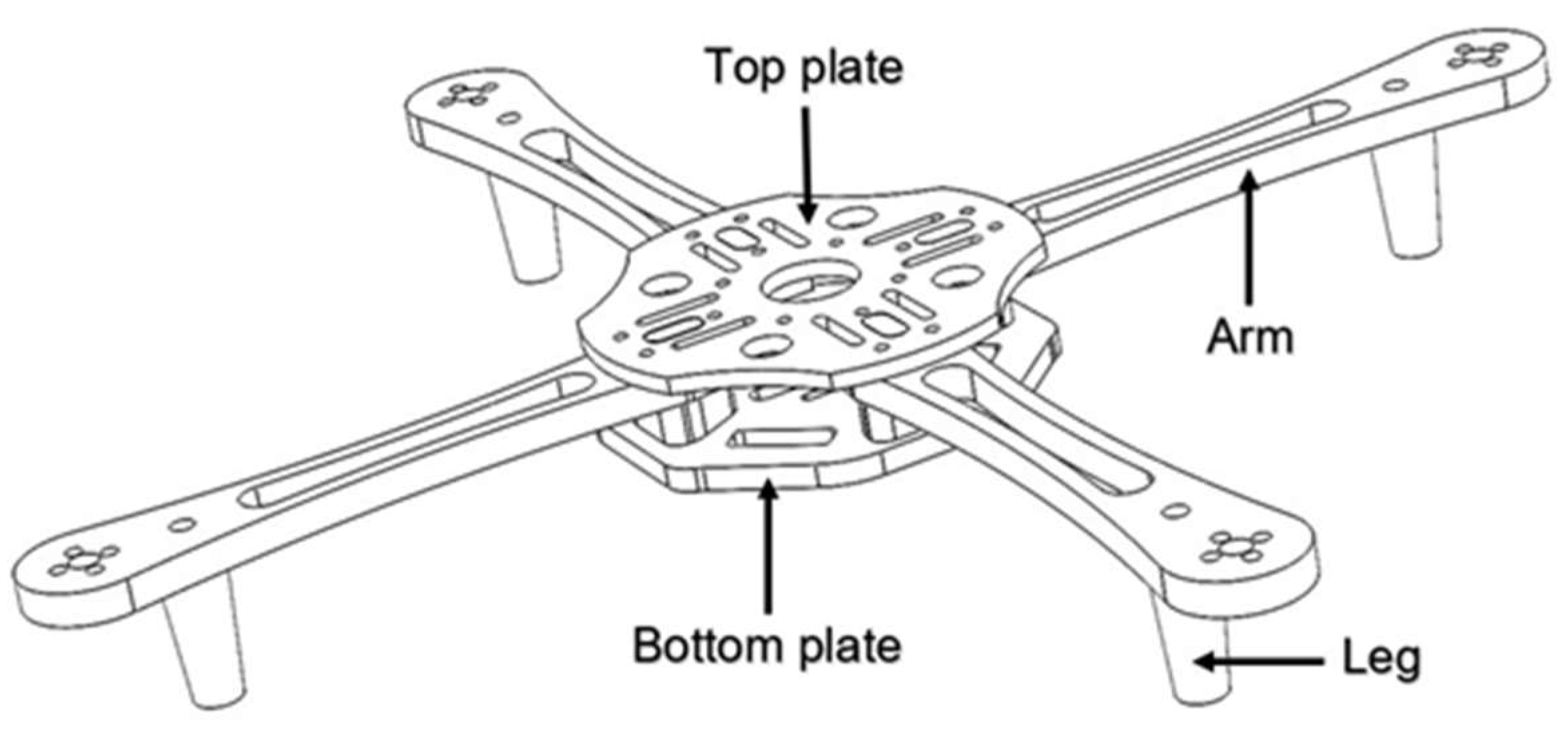
Figure 2.
Scheme of the threaded inserts placement in the drone arm.
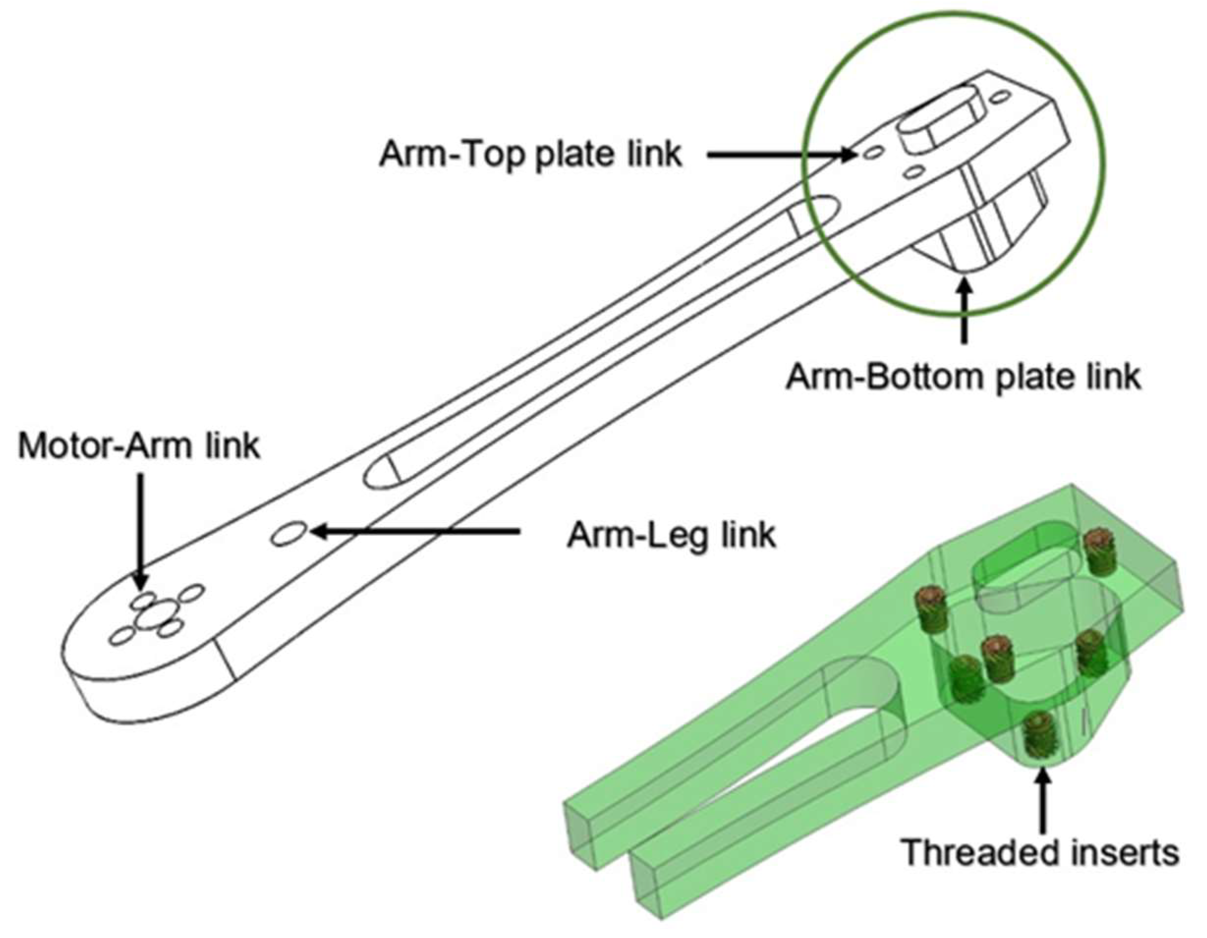
Figure 3.
Heat staking process: a) procedure schematic view; b) Final output.
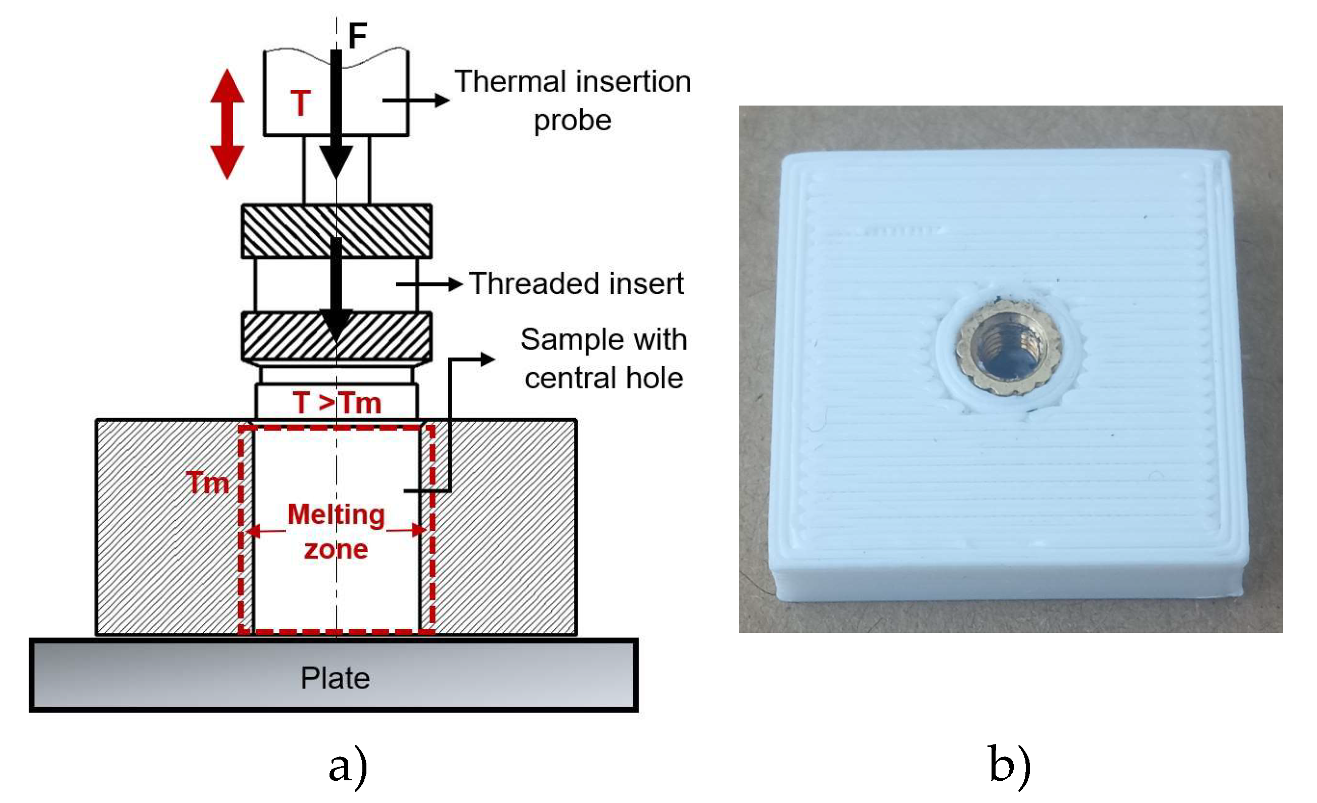
Figure 4.
The scheme of the sample and brass dimensions.
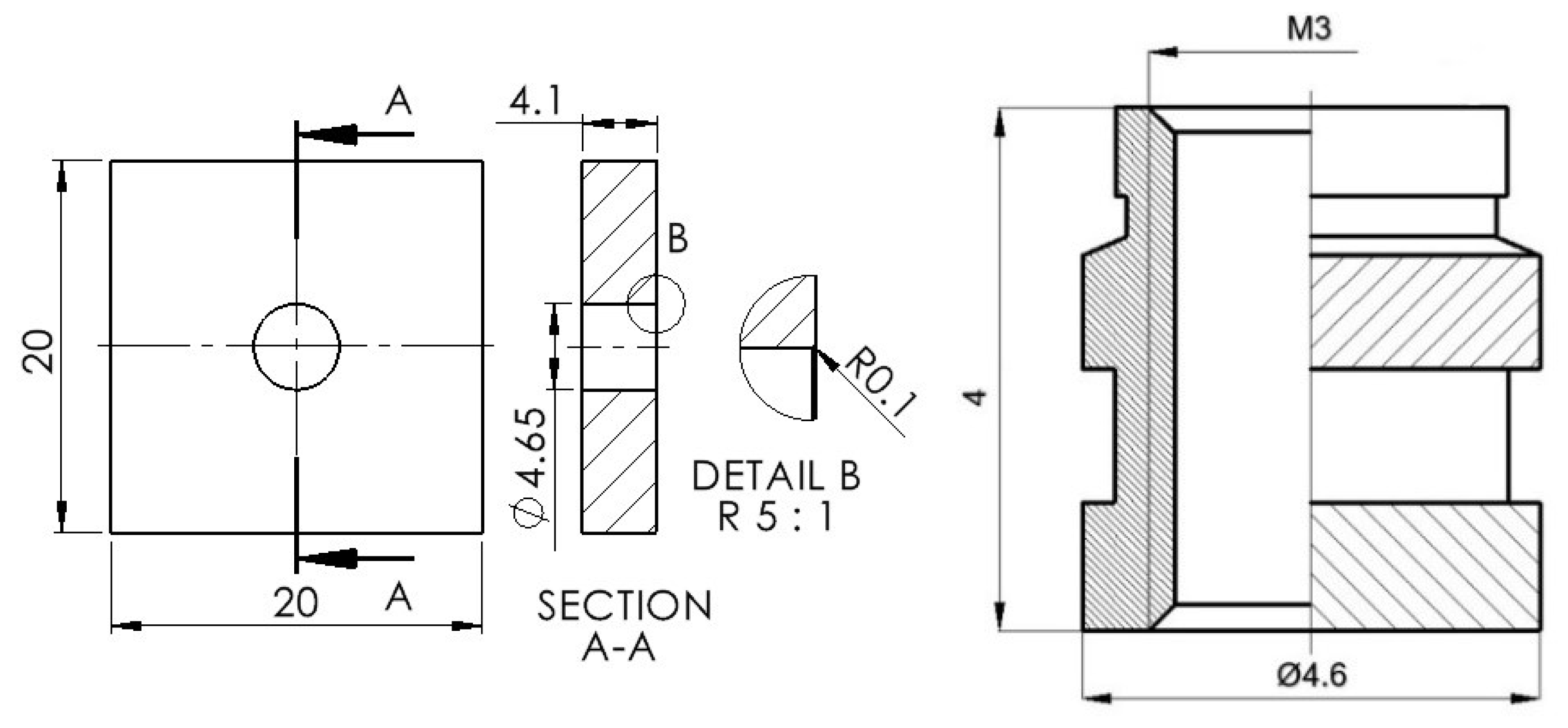
Figure 5.
Adapter tool: a) 3D model, b) manufactured model, c) setting.
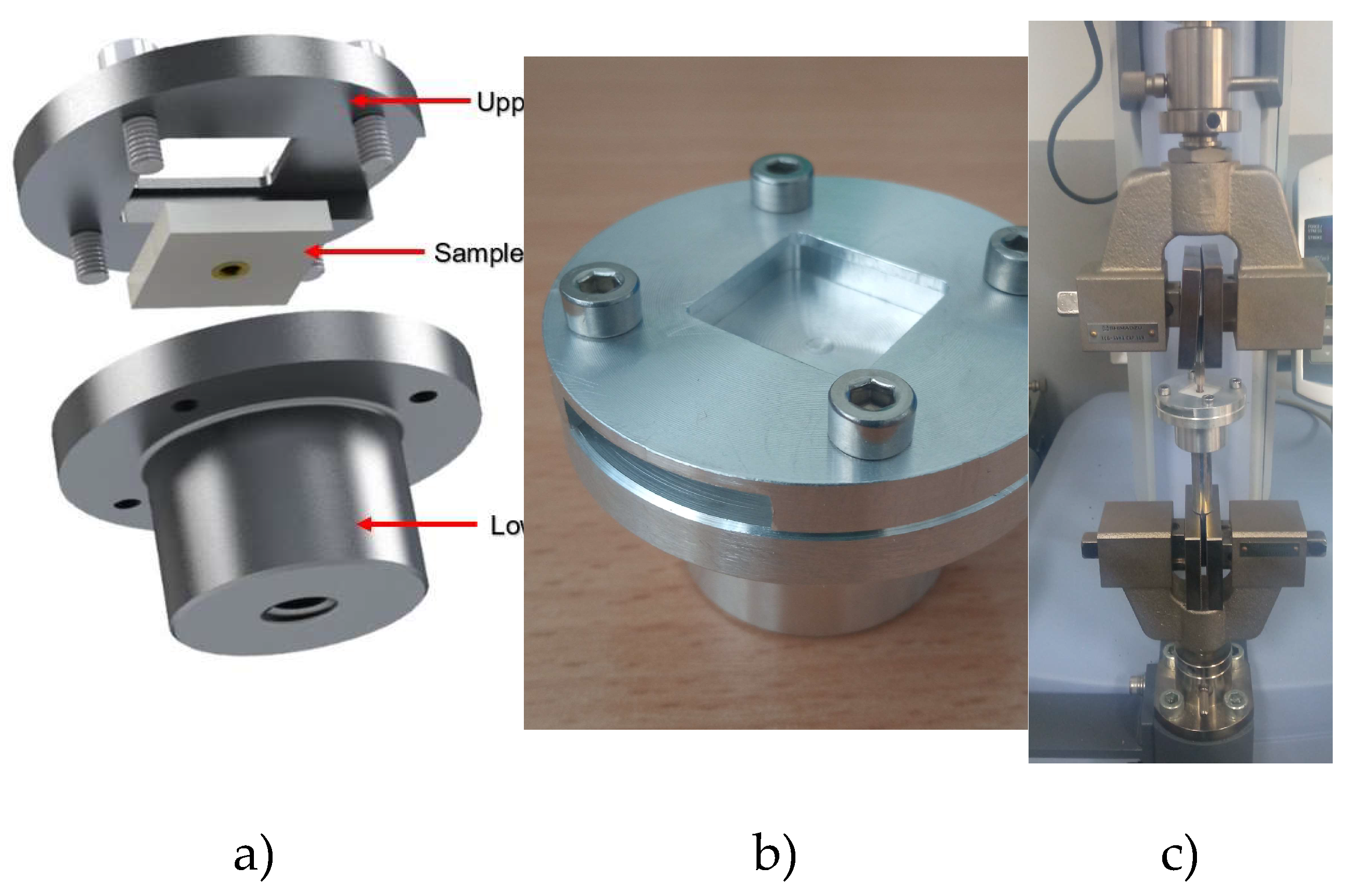
Figure 6.
Preview of test panels: a) settings, b) the second artificial aging.
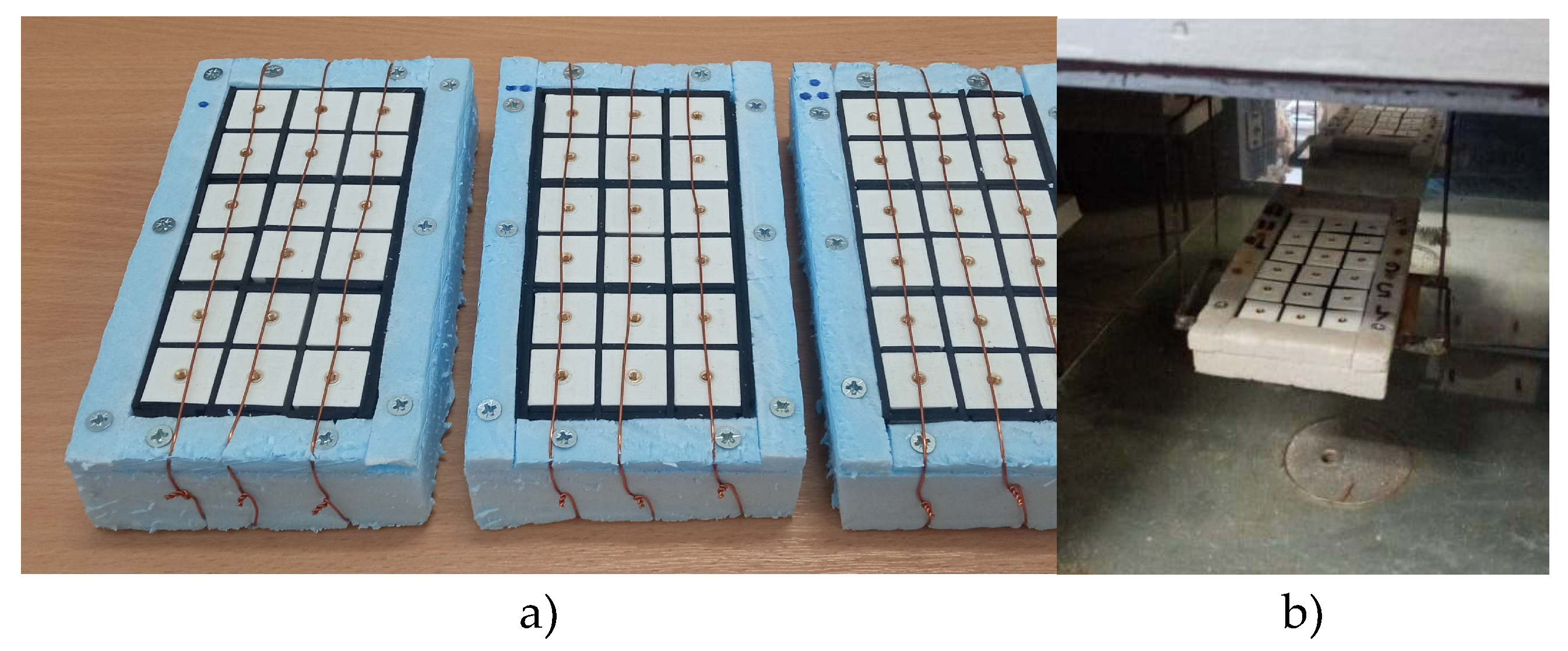
Figure 7.
Concentrated load position and drone arm dimensions.
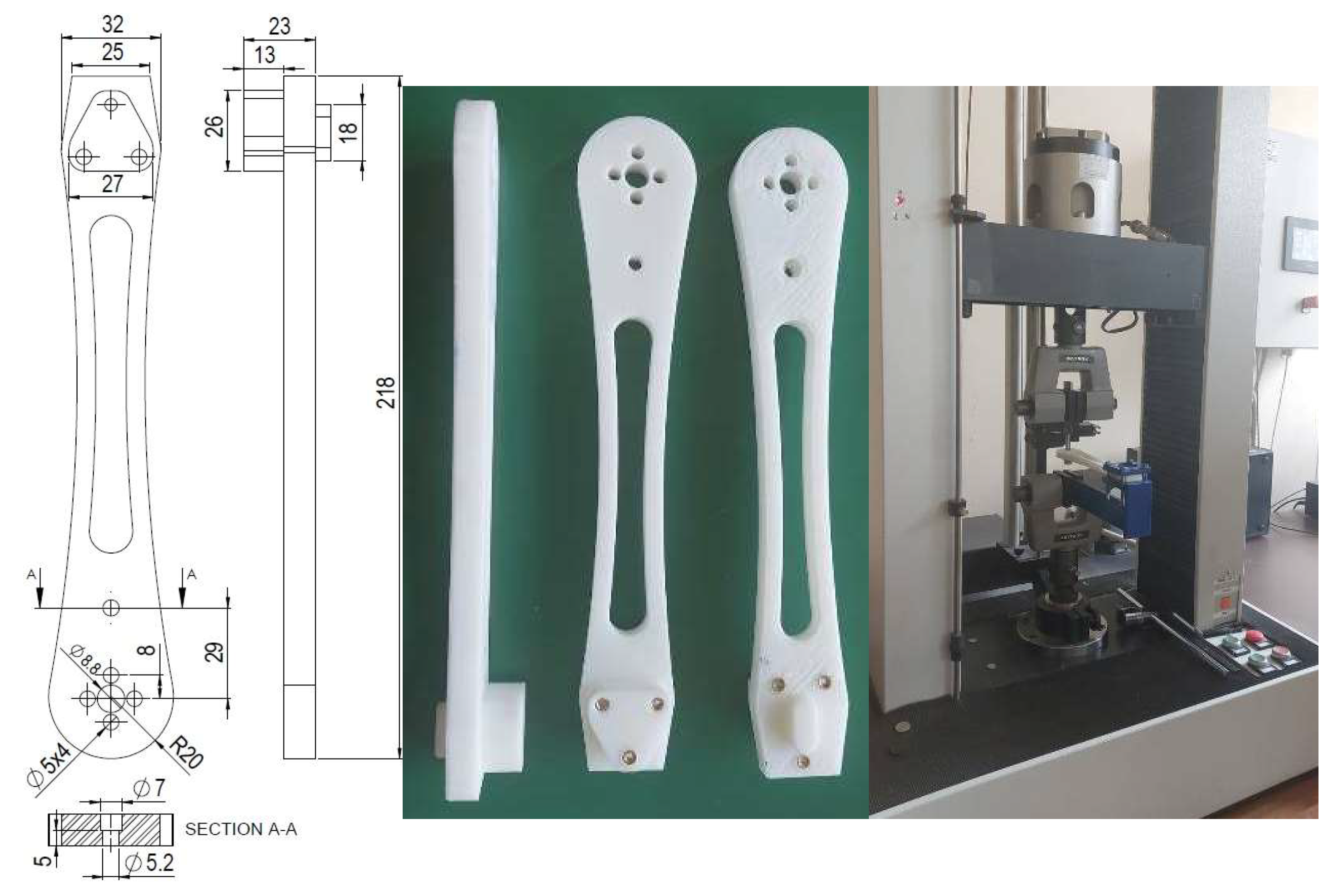
Figure 8.
Drop of pull-out force in treated samples in comparison to the SP.
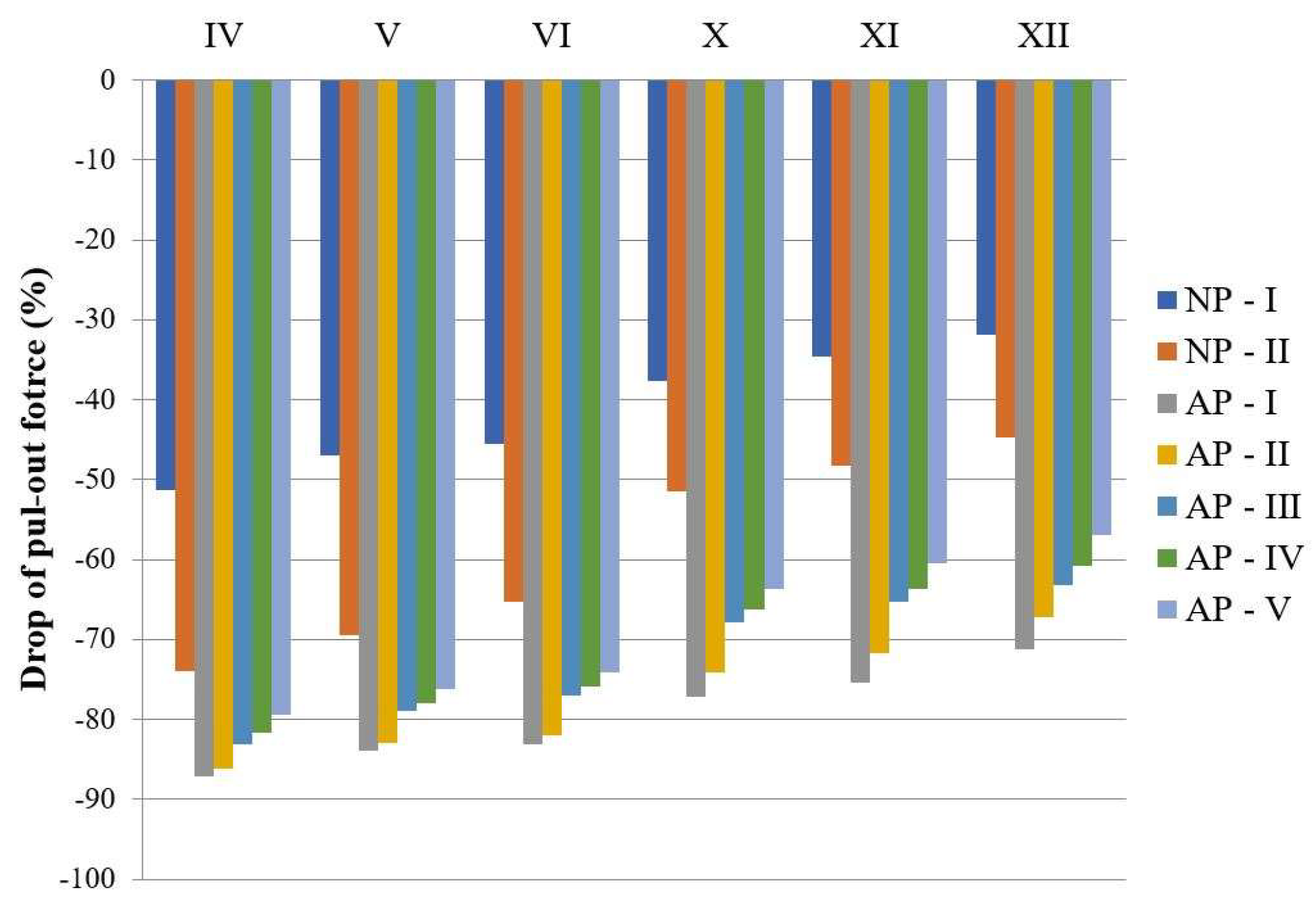
Figure 9.
Nozzle trajectory during printing samples IV – VI.

Figure 10.
The morphology of the tested samples after the pull-out test for NP-II, AP-III and AP-V.
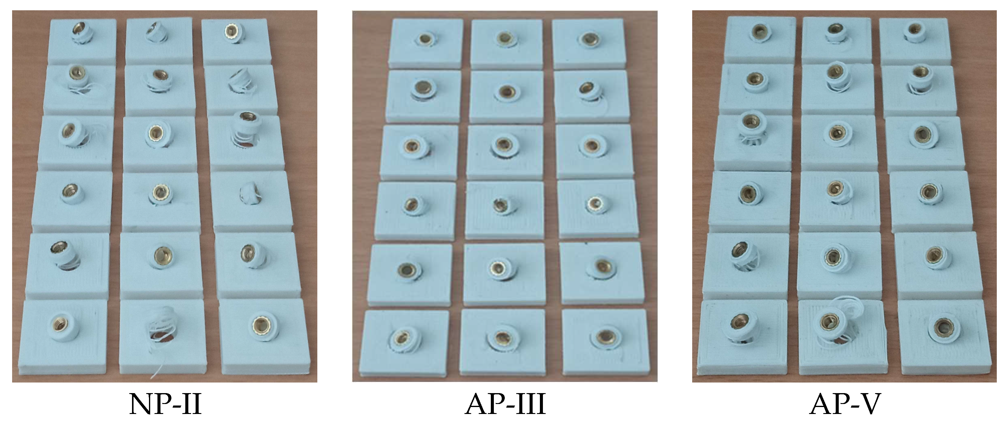
Figure 11.
The appearance of samples AP-II after pull-out test.
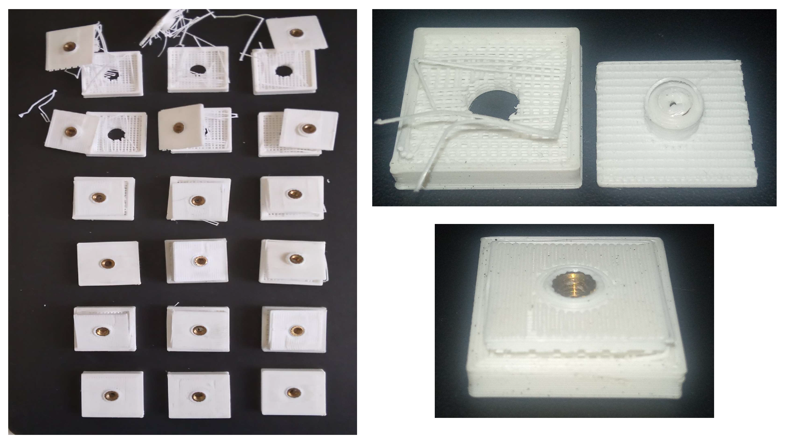
Figure 12.
FTIR analysis conducted before aging (base line – 0 days data set).
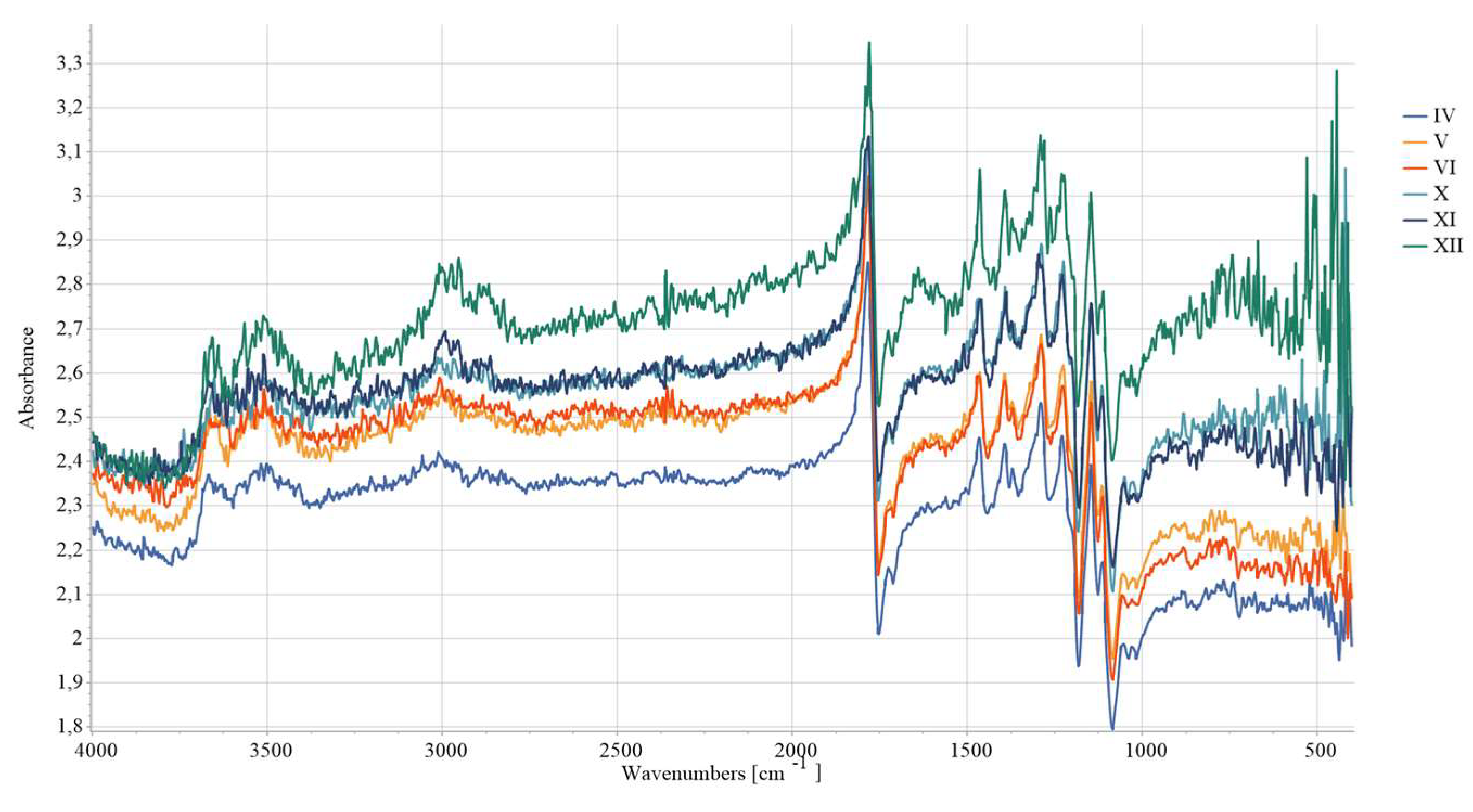
Figure 13.
FTIR analysis conducted after 44 days.
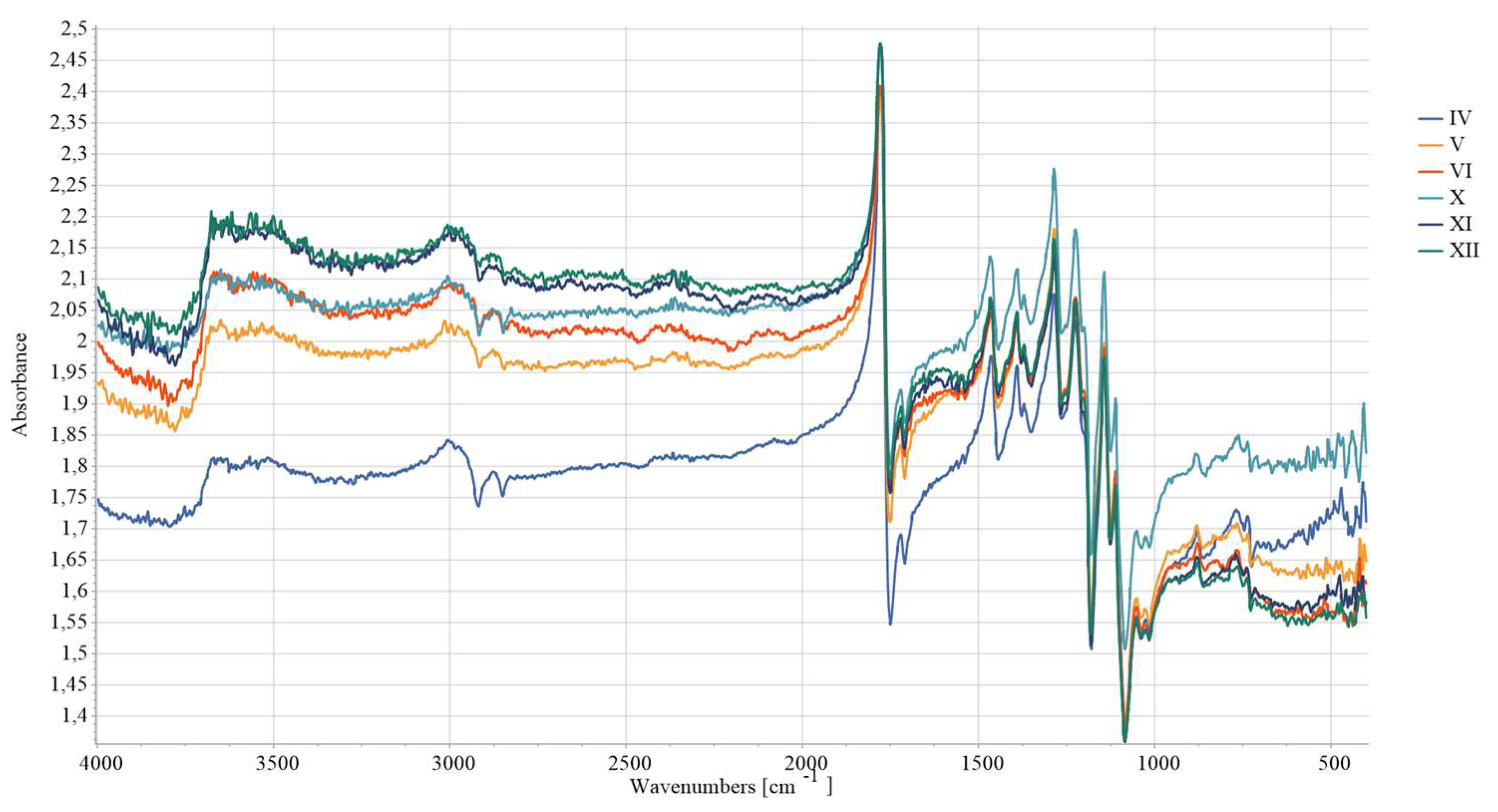
Figure 14.
FTIR analysis conducted for the sample IV.
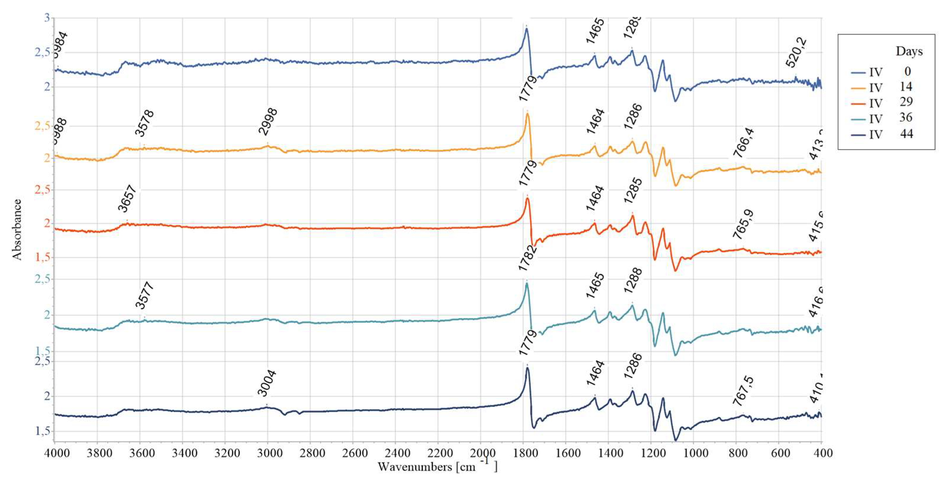
Figure 15.
FTIR analysis conducted for the sample XII.
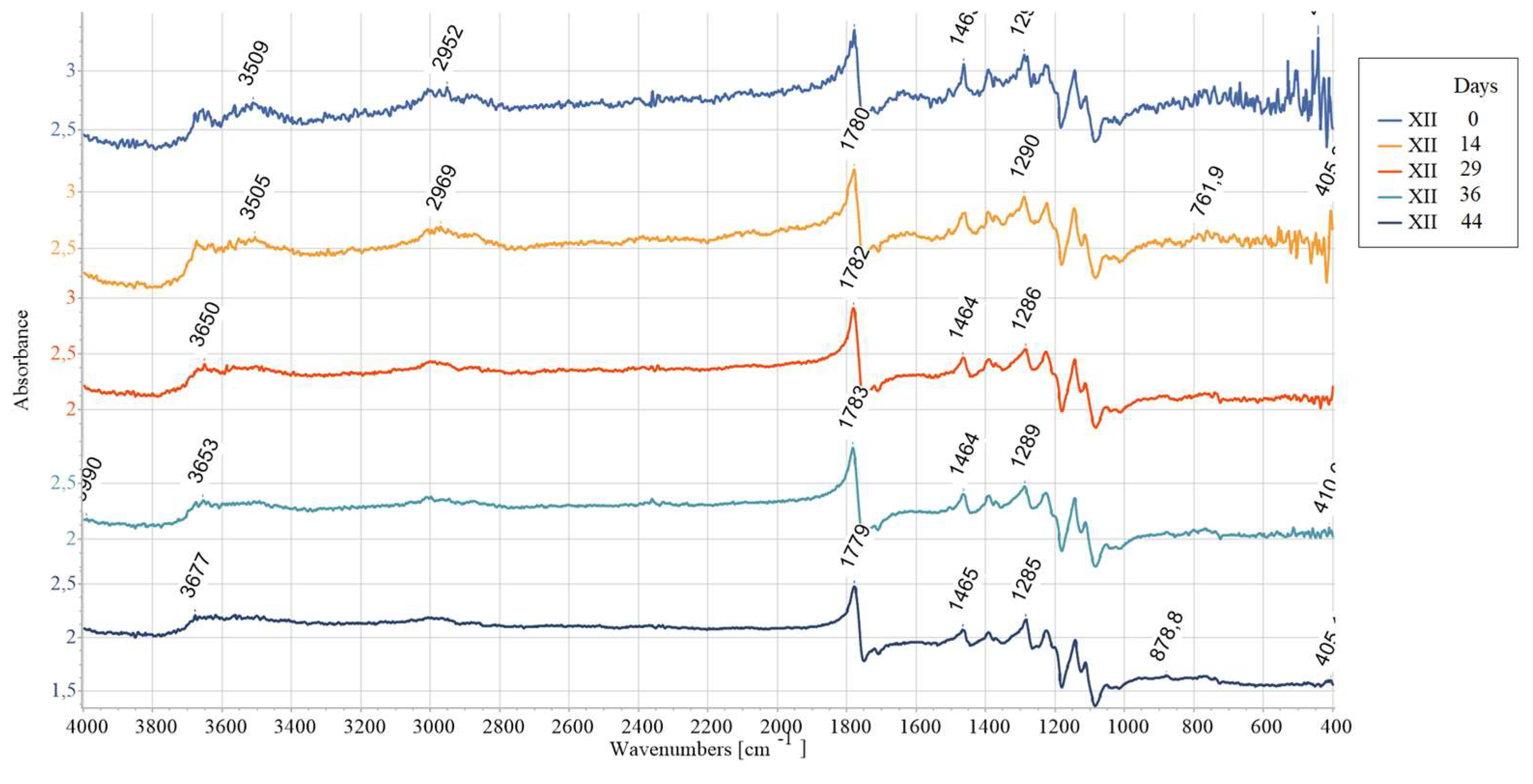
Figure 16.
Change of L during aging.
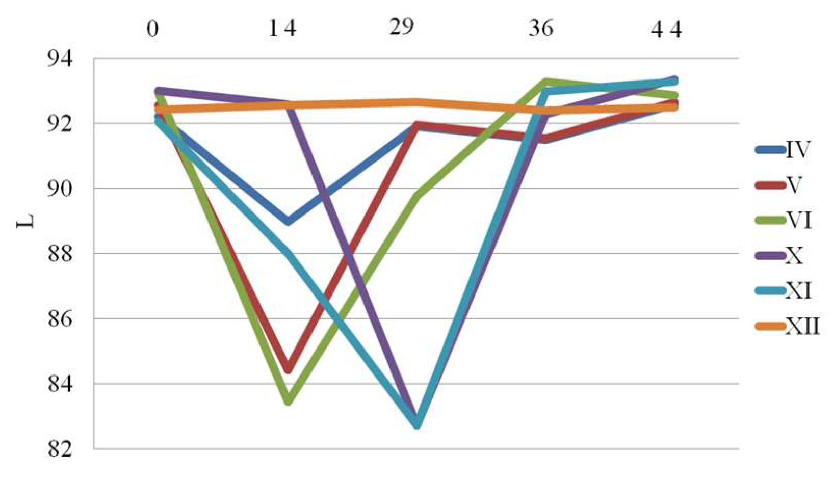
Figure 17.
Change of a during aging.
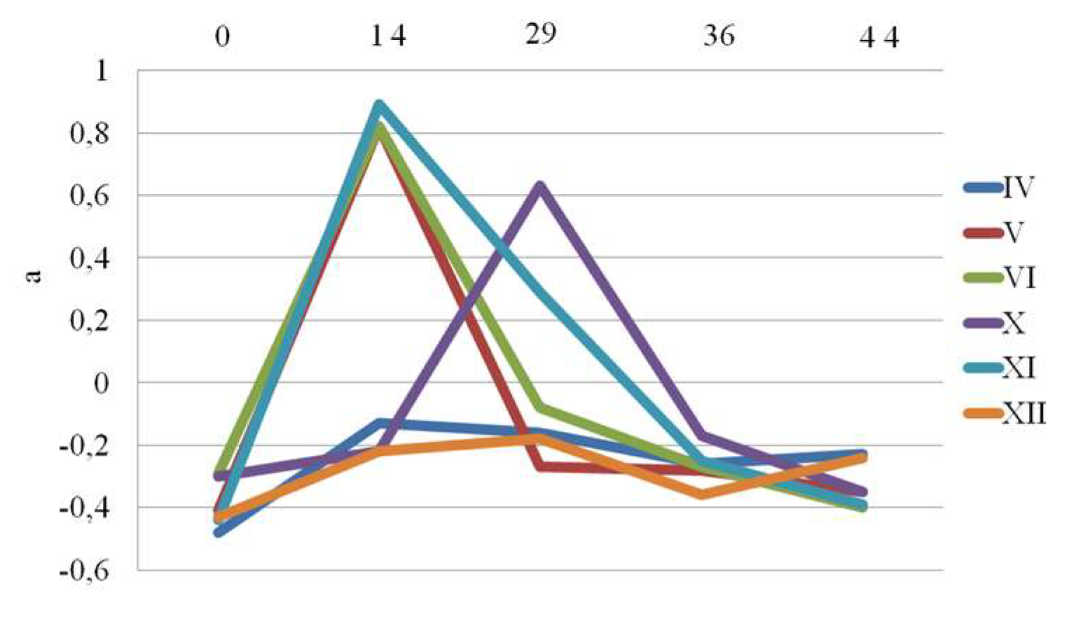
Figure 18.
Change of b during aging.
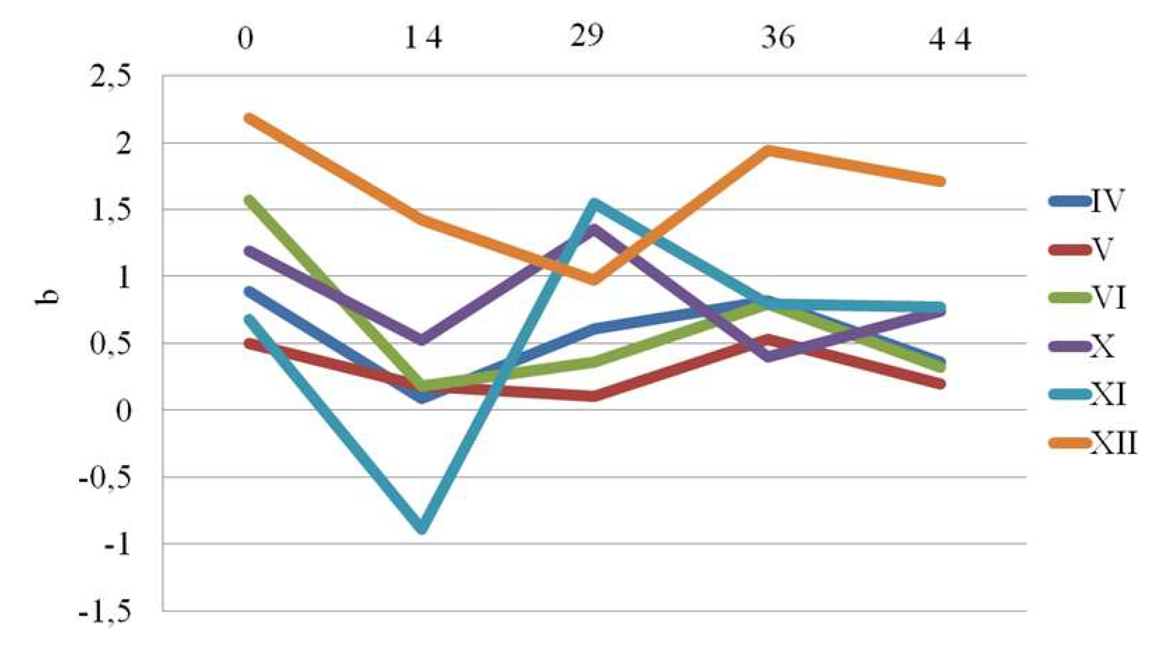
Figure 19.
Color difference ∆E.
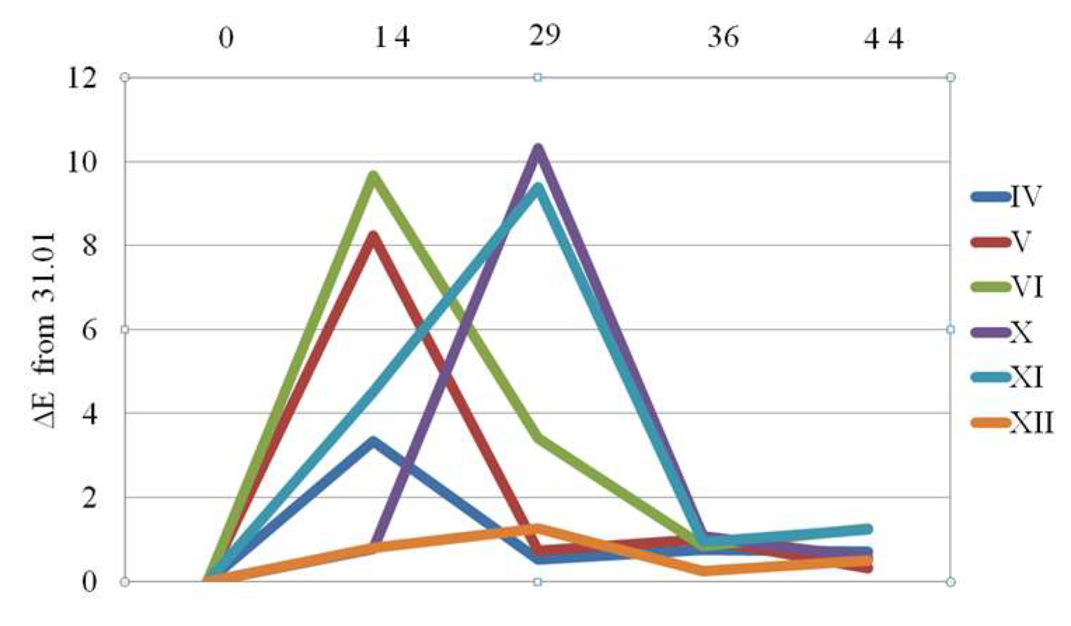
Figure 20.
Change of contact angle during aging.
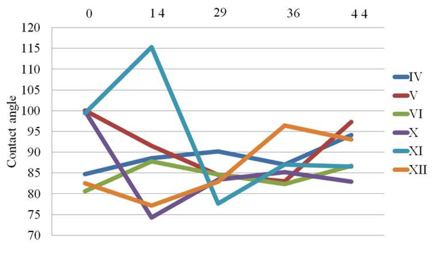
Figure 21.
Tensile (a) and concentration load (b) results.
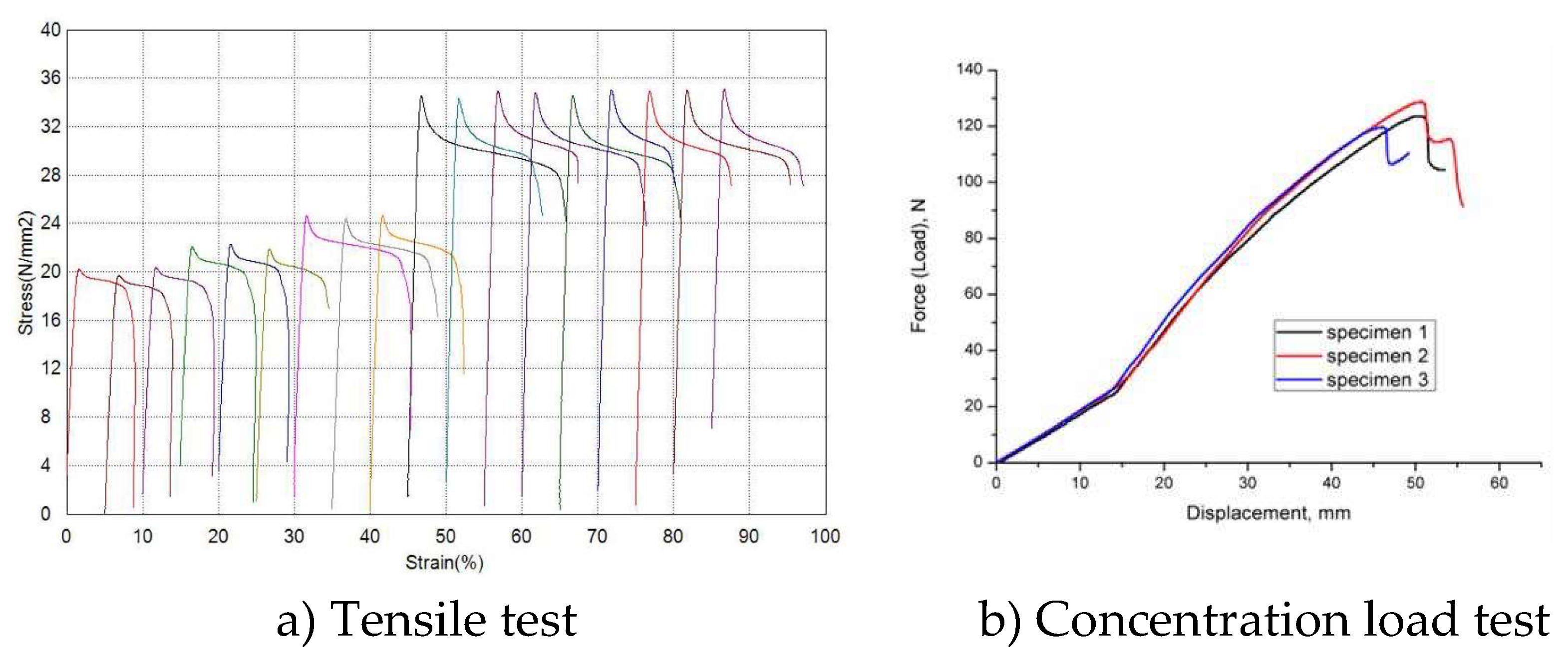
Figure 22.
The sample morphology after tensile (a), and concentration load (b).
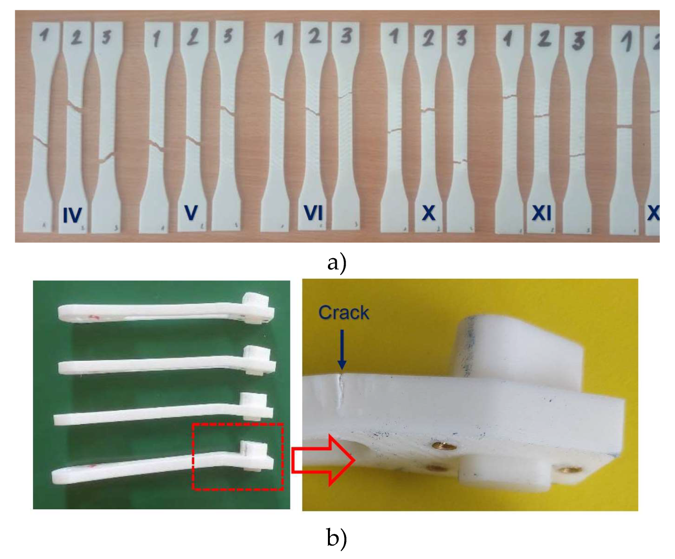
Figure 23.
Isometric view of the numerical model of the drone arm.
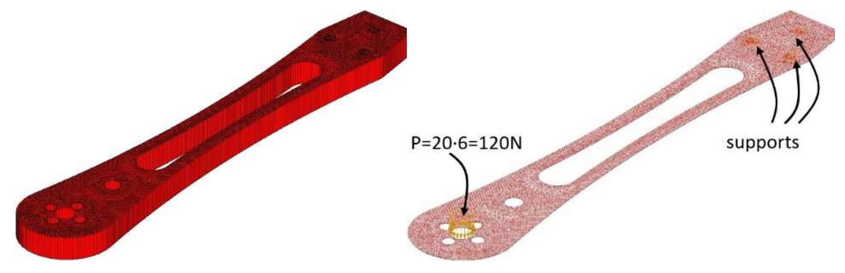
Figure 24.
Generated finite element mesh.
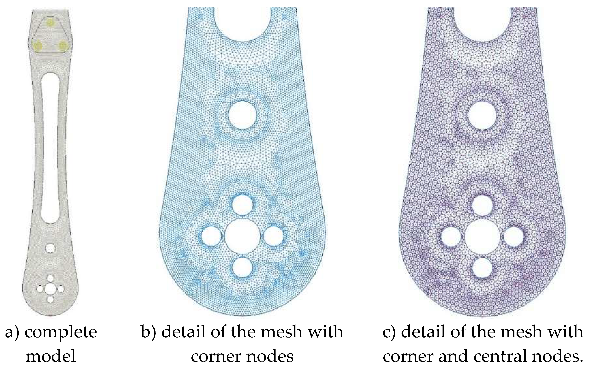
Figure 25.
The stress state iso-surface (top surface of the leg) for a force increment of 0.1·P.
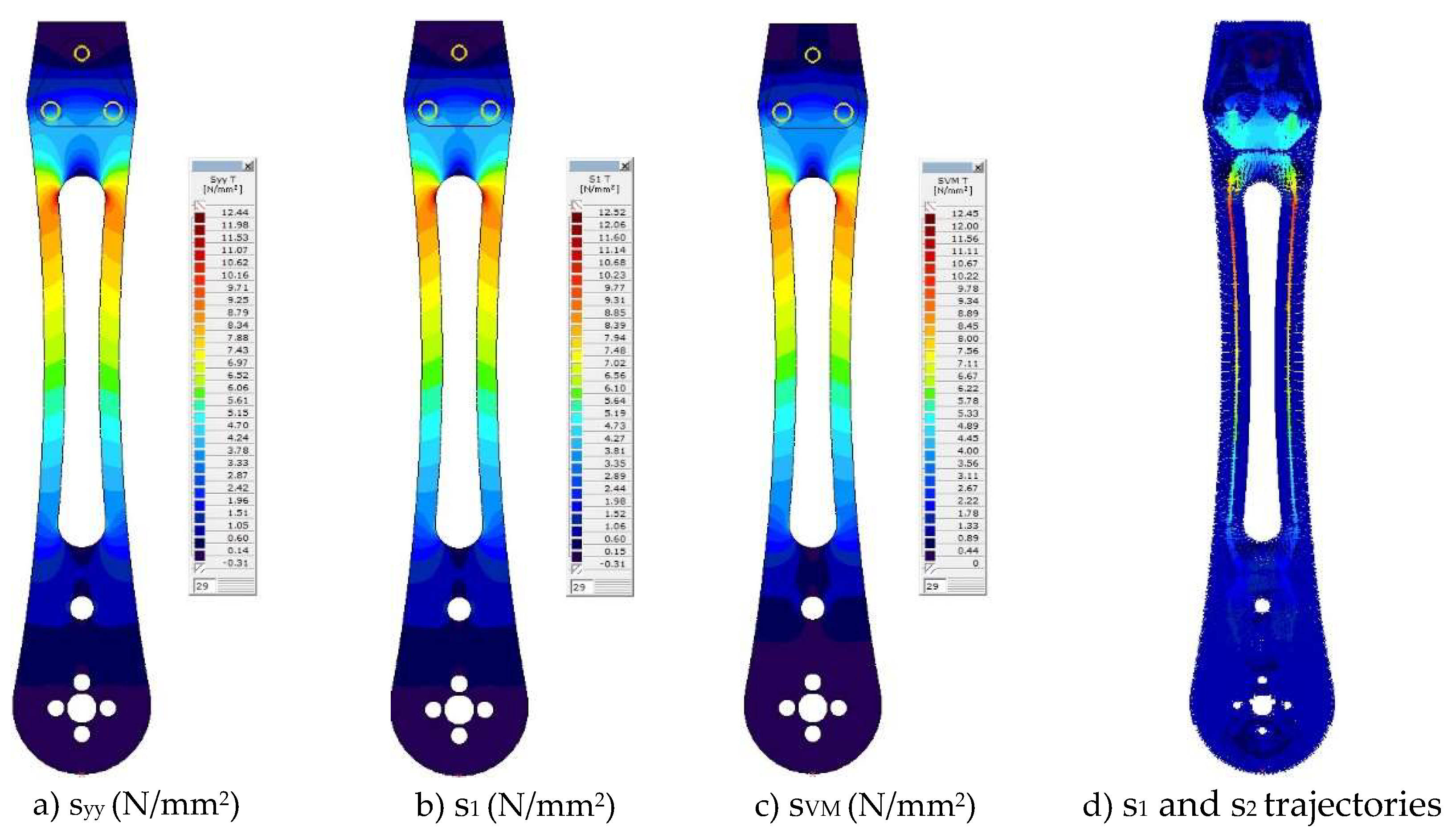
Figure 26.
Von Mises stress state iso-surface (arm top surface) for various force increments.
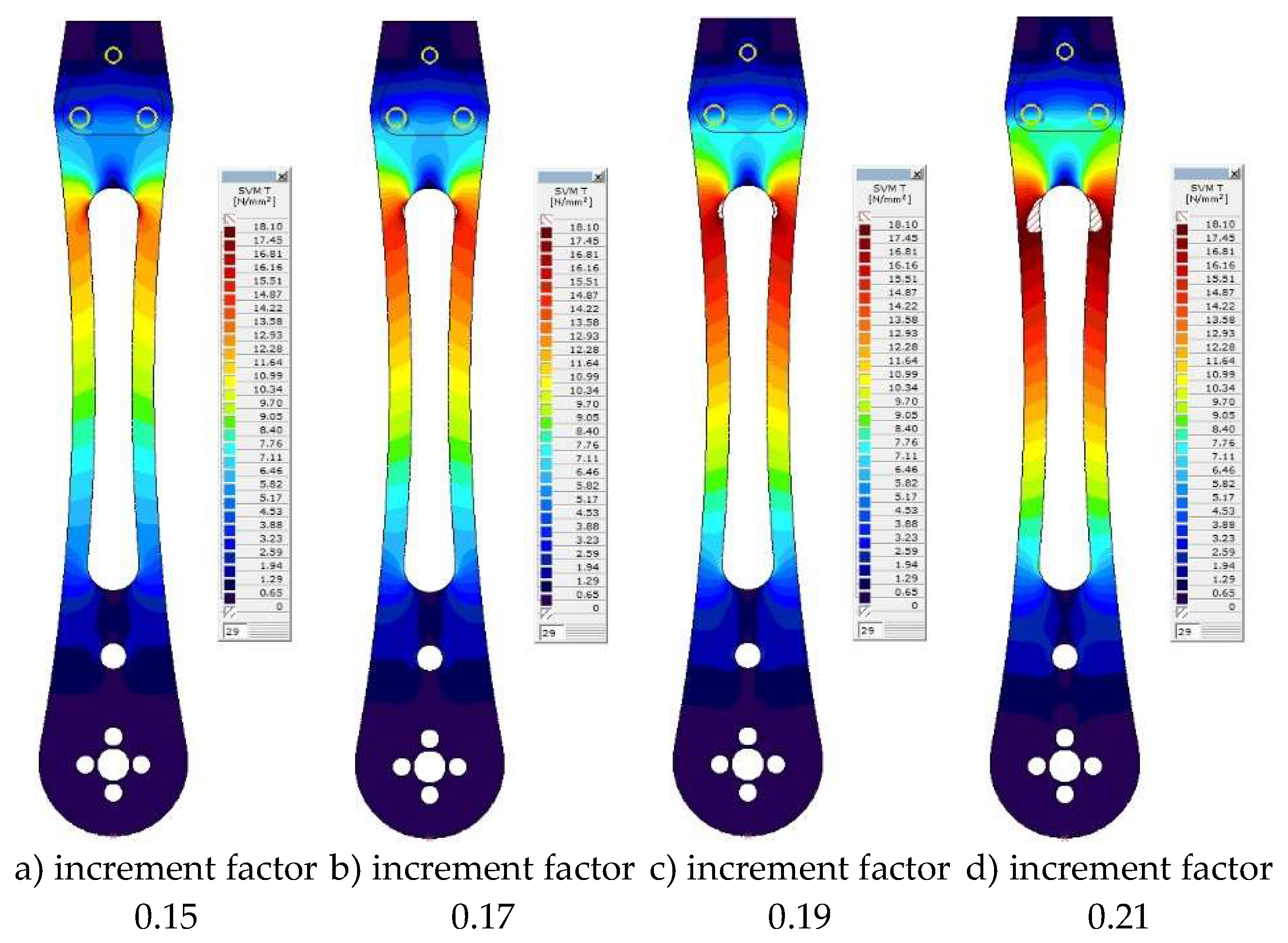
Figure 27.
Von Mises stresses in the section where yielding occurs for various the scaling factors.
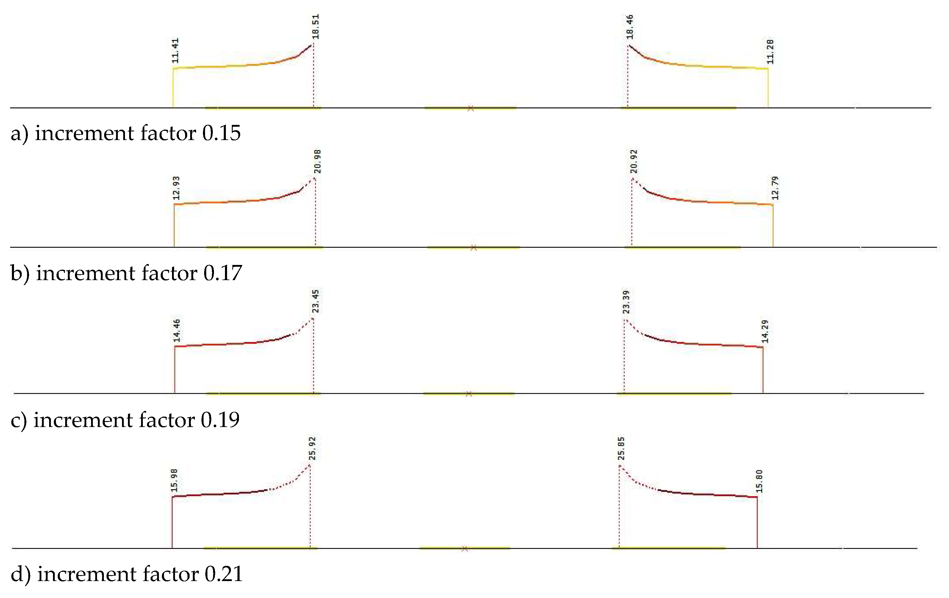

Table 1.
Printing parameter combinations.
| Samples designation code | IV | V | VI | X | XI | XII |
|---|---|---|---|---|---|---|
| Wall thickness [mm] | 0.8 | 1.2 | 1.6 | 0.8 | 1.2 | 1.6 |
| Wall line contour | 2 | 3 | 4 | 2 | 3 | 4 |
| Top layer number | 2 | 2 | 2 | 4 | 4 | 4 |
| Bottom layer number | 2 | 2 | 2 | 4 | 4 | 4 |
Table 2.
The results of the pull-out tests after natural and artificial aging.
| Designation code | Pull-out force [N] | |||||||
|---|---|---|---|---|---|---|---|---|
| SP | NP-I | NP-II | AP-I | AP-II | AP-III | AP-IV | AP-V | |
| IV | 433 | 211 | 113 | 55 | 60 | 73 | 79 | 89 |
| V | 442 | 235 | 135 | 71 | 75 | 93 | 97 | 105 |
| VI | 505 | 275 | 175 | 85 | 91 | 116 | 122 | 131 |
| X | 578 | 360 | 280 | 132 | 149 | 186 | 195 | 210 |
| XI | 619 | 405 | 320 | 152 | 175 | 215 | 225 | 245 |
| XII | 624 | 425 | 345 | 179 | 205 | 230 | 245 | 269 |
Table 3.
Tensile test results.
| Sample | Max. Stress, σ (N/mm2) | Strain at Max. Stress, ε (%) | Modulus, E (N/ mm2) |
|---|---|---|---|
| IV-1 | 18.07 | 8.22 | 1056 |
| IV-2 | 17.70 | 7.92 | 1605 |
| IV-3 | 18.07 | 8.59 | 1253 |
| V-1 | 19.23 | 9.19 | 1276 |
| V-2 | 19.41 | 8.43 | 1083 |
| V-3 | 18.51 | 9.20 | 1762 |
| VI-1 | 20.28 | 14.48 | 1416 |
| VI-2 | 20.22 | 12.95 | 1853 |
| VI-3 | 20.26 | 11.57 | 2851 |
| X-1 | 27.18 | 20.30 | 3522 |
| X-2 | 28.52 | 11.61 | 2520 |
| X-3 | 28.79 | 12.42 | 2705 |
| XI-1 | 28.12 | 15.64 | 2962 |
| XI-2 | 27.78 | 15.19 | 5691 |
| XI-3 | 28.86 | 9.84 | 2375 |
| XII-1 | 28.24 | 12.44 | 2901 |
| XII-2 | 28.04 | 15.38 | 2388 |
| XII-3 | 28.52 | 11.94 | 2800 |
Table 4.
Allowed concentration loads.
| Sample | IV | V | VI | X | XI | XII |
|---|---|---|---|---|---|---|
| ACL with confidence level 10 per drone arm (kg) | 1,59 | 1,67 | 1,78 | 2,48 | 2,50 | 2,70 |
| ACL with confidence level 20 per drone arm (kg) | 1,46 | 1,53 | 1,63 | 2,38 | 2,29 | 2,31 |
| Drone payload capacity with confidence level 10 (kg) | 6.36 | 6.68 | 7.12 | 9.92 | 10 | 10.8 |
| Drone payload capacity with confidence level 20 (kg) | 5.84 | 6.12 | 6.52 | 9.52 | 9.16 | 9.24 |
Table 5.
Drone size classification.
| Drone size | Payload capacity | Description |
|---|---|---|
| Mini drones | ≤ 100 g | Recreational use. |
| Small drones | 100g – 1kg | Recreational or light commercial tasks |
| Medium drones | 1 – 5 kg | Professional use (photography, surveying, agricuture) |
| Large drones | 5 – 30 kg | Industrial use (inspections, cargo transport, etc.) |
| Heavy lift drones | ≥ 30 kg | Heavy lifting in construction, agriculture or emergency operations |
Table 6.
Preset printing parameter combinations.
| Designation code | I | II | III | IV | V | VI | VII | VIII | IX | X | XI | XII |
|---|---|---|---|---|---|---|---|---|---|---|---|---|
| Layer height [mm] | 0.1 | 0.1 | 0.1 | 0.3 | 0.3 | 0.3 | 0.1 | 0.1 | 0.1 | 0.3 | 0.3 | 0.3 |
| Wall thickness [mm] | 0.8 | 1.2 | 1.6 | 0.8 | 1.2 | 1.6 | 0.8 | 1.2 | 1.6 | 0.8 | 1.2 | 1.6 |
| Wall line contour | 2 | 3 | 4 | 2 | 3 | 4 | 2 | 3 | 4 | 2 | 3 | 4 |
| Top layer number | 2 | 2 | 2 | 2 | 2 | 2 | 4 | 4 | 4 | 4 | 4 | 4 |
| Bottom layer number | 2 | 2 | 2 | 2 | 2 | 2 | 4 | 4 | 4 | 4 | 4 | 4 |
Disclaimer/Publisher’s Note: The statements, opinions and data contained in all publications are solely those of the individual author(s) and contributor(s) and not of MDPI and/or the editor(s). MDPI and/or the editor(s) disclaim responsibility for any injury to people or property resulting from any ideas, methods, instructions or products referred to in the content. |
© 2025 by the authors. Licensee MDPI, Basel, Switzerland. This article is an open access article distributed under the terms and conditions of the Creative Commons Attribution (CC BY) license (http://creativecommons.org/licenses/by/4.0/).
Copyright: This open access article is published under a Creative Commons CC BY 4.0 license, which permit the free download, distribution, and reuse, provided that the author and preprint are cited in any reuse.


