Submitted:
22 April 2025
Posted:
22 April 2025
You are already at the latest version
Abstract
A theoretical model is presented for the accurate detection of gas leak source through a pinhole in a cylindrical storage vessel using the acoustic emission (AE) technique. Pinholes of various diameters ranging from 0.20 to 1.2 mm were installed as leak sources, and safe N2 was used as a filler gas. AE parameters such as frequency, amplitude, and RMS of the AE signal generated by the gas leak were measured. Among them, the amplitude characteristic was the most important parameter to determine the leak dynamics of AE with continuous waveform. The amplitude of the AE signal generated by the leak was investigated as a function of angle and axial distance, and the simulation was performed using the theoretical model for AE. For practical applications, the theoretical formula was modified into two semi-empirical equations by introducing the normalization method to fit the angular and axial characteristics of the observed AE amplitude, respectively. The main advantage of this study is that the semi-empirical equations provide an accurate solution for leak source localization in the cylindrical vessel. As a priori knowledge, the value of κη in Green’s function, which determines the angular and axial dependence of the AE amplitude, was determined by applying external excitation to the cylinder surface. The proposed formulas provide a suitable approach for practical application in the localization of leak source in cylindrical storage tanks.
Keywords:
acoustic emission
; amplitude
; analytical modeling
; semi-empirical equation
; leak source localization
1. Introduction
Cylindrical vessels are more commonly used as pressure vessels than spherical vessels due to their ease of fabrication, space utilization, pressure resistance and ease of maintenance. In a confined space, cylindrical tanks are very effective for the storage and use of fuel gases due to their ease of transport, high storage capacity and pressure regulation. The need for reliable maintenance of high-pressure gas cylinders and tanks, especially those containing hazardous gases, has increased exponentially over the past decade due to the high potential for safety hazards from leaks caused by undetected vessel damage. The most important way to prevent disasters caused by gas leaks is to detect the leak and its location and repair it accordingly. Several leak detection methods have been proposed for the early detection of leaks in pipelines [1]. These include acoustic emission (AE) detection, flow rate or pressure monitoring, or infrared detection [2,3,4,5,6,7,8]. Among the various methods, AE methods have proven to be very effective in detecting and locating leaks by eliminating interfering signals through time and frequency domain analysis and characterization of AE parameters [9,10,11,12].
In general, the most notable methods for locating an AE source are the time domain technique and the zone location technique [13]. The former relies on the time difference of arrival (TDOA) between two or more AE sensors to derive the source location [14]. However, the time delay can also result from different wave paths, different wave modes due to the dispersion of the AE wave for a long-distance pipeline and the velocity variation due to the environment. Therefore, the TDOA technique requires high detection accuracy. However, because the TDOA method is applied to burst-shaped waveforms, it is not suitable for locating leak sources in the case of leaks that produce continuous AE waveforms. To overcome this, the cross-correlation algorithm is sometimes used to obtain the TDOA from continuous waveforms [15,16]. Due to background noise and other uncertainties during the measurement, achieving a good level of correlation coefficient is limited [10,17]. In practical situations, the AE signal generated by a leak has an aperiodic waveform structure and the exact location of the leak source cannot be determined by the cross-correlation based methods. The second one of the basic AE localization techniques is based on the attenuation of the AE amplitude with the distance between the leak source and the detection sensor, taking advantage of the fact that the sensor with the largest amplitude is closest to the leak source, assuming that the sensitivity of the sensors is the same. However, this method has limitations in pinpointing the location of the leak in three dimensions because it ignores the influence of the AE signal due to the structural characteristics of the vessel. To overcome this drawback, AE signal analysis is required using governing equations that take into account the structural characteristics of the storage vessel and the propagation dynamics of AE caused by leaks on the vessel surface. In addition, this method can only be used if the structure has a moderate attenuation of the AE signal. This technique can provide a simple solution where the exact location of the leak source is not critical.
Over the past few decades, numerous studies have been conducted to solve the problems of pipeline leak localization using acoustic-based methods [10,12]. However, there are still limitations and gaps in fundamental research dealing with signal modelling, nonlinear effects and environmental uncertainty in leak AE signals [10]. Previously, a mathematical formula was formulated for AE generated by a point source (PS) as an internal defect in cylindrical structures [18]. The PS was represented by a concentrated force (CF) with both spatial and temporal harmonic characteristics. In cylindrical geometry, the CF generates three potential functions representing a compression wave (P) and two shear waves (horizontal and vertical polarization, SH and SV, respectively), which are referred to as the concentrated force-incorporated potential (CFIP). The radial, tangential and axial displacements were solved by introducing the CFIPs into the Navier-Lamé (NL) equation, based on the model proposed by Morse and Feshbach [19]. Previously, the CFIPs for the pinhole leakage were derived as an excitation AE source, associated with a fluctuating Reynolds stress (FRS) [20]. As the FRS acts on the pinhole wall, the CFIP due to the FRS results only in the axial and tangential displacements. A limited investigation of the angular and axial dependence of the AE signals for the pinhole leakage source has been carried out. The characteristics of the observed AE signals due to the pinhole leakage were well simulated by the proposed theoretical formula. The aim of this study is to investigate the feasibility of applying the proposed mathematical model to leakage source localization in cylindrical geometries. Detailed measurements of the AE signals generated by leakages through pinholes of different diameters in gas cylinders were performed. For application to leak source (LS) localization, the theoretical formula was modified into two semi-empirical equations to describe the angular and axial dependence of the observed AE amplitude, respectively. Finally, the simulation and experimental results were compared to verify the accuracy of the leak source localization.
2. Mathematical Solution
2.1. Concentrated Forces
In general, the CF as the PS excitation of the AE is described as
where P is the force vector acting at and is the angular frequency that transfers the AE energy from the PS to a solid space. In Eq. (1), the delta function provides the spatial distribution of the CF at a given time as Green’s function defined as The CF generated by the PS can be rewritten in terms of vectors as
or
The derivation of the Green’s function for the cylindrical cell structure [18,20,21] is summarized in Appendix A. Applying the periodicity of 2π (= 0) to Eqs. (A17)–(A19) gives
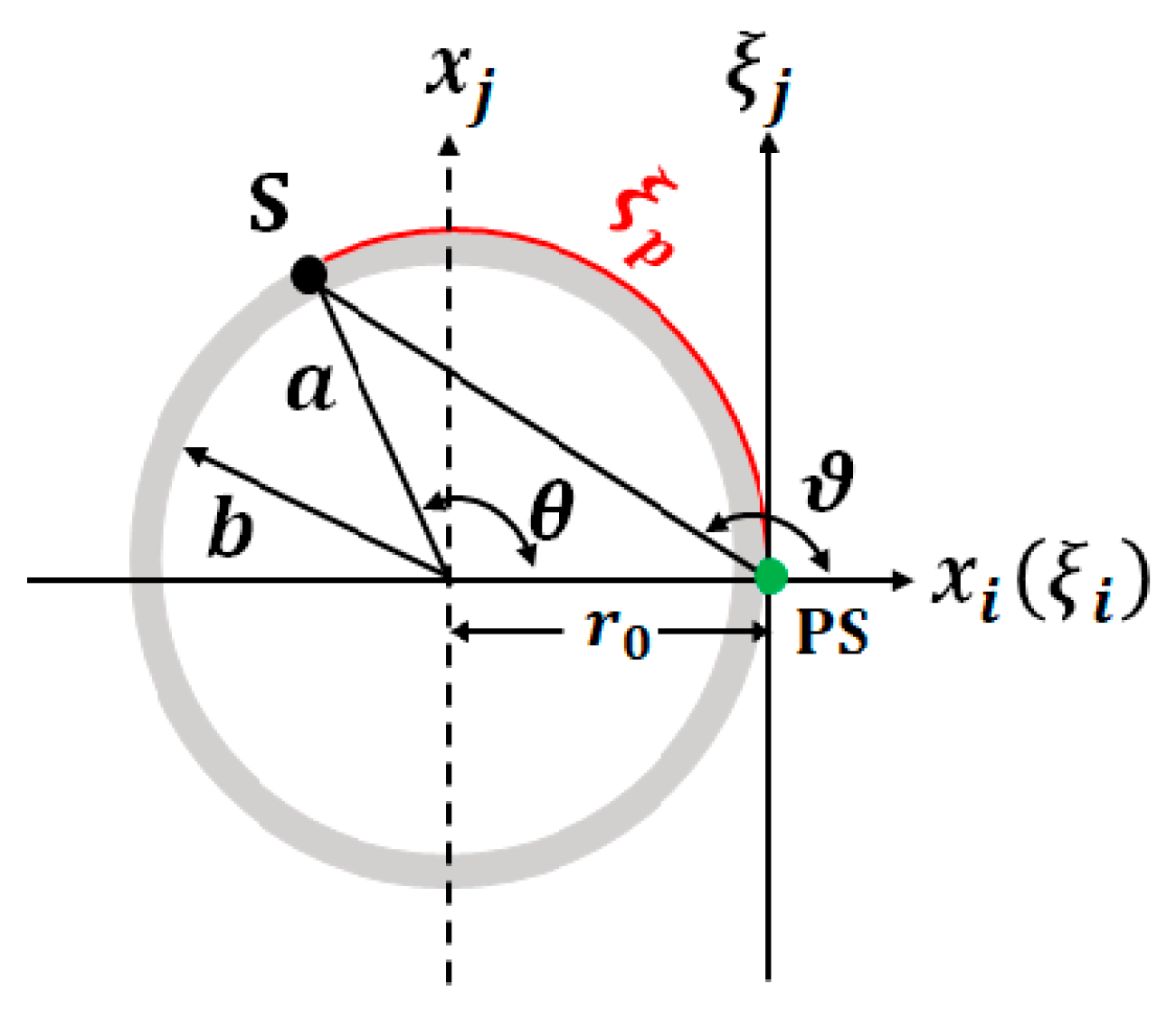
where the PS is located at and . In Eq. (3), the value of is the shortest distance between the PS and the detection point on the cylinder surface (Figure A1). If the thickness is much shorter than the diameter of the outer circle, the value of can be given as the length of the arc around the outer circle,
where the PS and the detector are located on the outer surface of the cylinder (Notes. Corrects a typographical error in inserted in Figure 2b of Ref. 20). In Refs. 18 and 21, the value of was determined by applying boundary conditions to the Bessel function in Eq. (A6). For the outer surface gives . On the other hand, in Ref. 20, the value of was determined experimentally from the angular dependence of the AE amplitude. The subscripts and n of and represent the azimuthal constant and the nth-order root in the boundary conditions, respectively. In this study, the value of was determined using the external excitation method: therefore, the subscript n was omitted in Eqs. (3)–(5).
The FRS is the most effective excitation source for AE due to fluid leakage through a pinhole. For turbulent flow with a radial turbulent velocity of through a circular hole in the cylindrical structure, the CF is exerted on the wall of the pinhole by the FRS. Denoting the fluctuating velocities along the axial (z) and tangential (θ) directions as and , respectively, the FRS at low Mach numbers is defined as
where ρ is the density of the charged gas. From Eq. (7), the force vectors acting on the pinhole wall are given by [22]
where the upper bar symbol represents the value averaged over a period of time. Since , . The CF vector can be written down as
From the reported data [23], the CF can be obtained as
where U is the mean velocity of and is given as Eq. (B5).
2.2. Displacement Fields
The displacement fields u generated by the CF in the cylindrical geometry can be derived by using the NL equation [24],
and the Morse and Freshbach’s model [19,25],
where λ and μ are Lamé constants and ρ is the density of the media. In Eq. (12), Φ is the scalar potential for the P wave, is vector potential for the SH wave, is vector potential for the SV wave, and a is the outer radius of the cylinder. Note that the velocities of the P and S waves are given as and , respectively.
For the PS excitation, the three potentials can be specified as the CFIPs. In coordinates, the three CFIPs are expressed as
where and are scalar functions for and , respectively. (Notes. Corrects the erratum in the sign of in Refs. 18 and 20.) The combination of Eqs. (2) and (13)–(15) gives a second-order partial differential equation (PDE) for each scalar function. The radial PDEs of and are nonhomogeneous, and their solutions are a linear combination of the homogeneous and the particular solutions. These three PDEs were solved by introducing for the imaginary roots of the axial component and as an azimuthal constant for the angular component. The solutions of the and functions are given by Eqs. (C1)–(C3). By substituting each scale function into the corresponding potential, the CFIPs can be obtained as expressed in Eqs. (C4)–(C9).
When the displacement is produced by the force component , u in Eq. (12) can be rewritten as the cylindrical components of the displacement
where
These three equations can be written as
where or and or for the pinhole leakage. In Eq. (20), the terms are given in Eqs. (C10)–(C15).
Since the Bessell functions and in the CFIPs become the unity as approaches to the PS, then m = 0. For m = 0, the terms are as follows: for (radial component),
(tangential component)
(axial component)
for ,
(radial component)
(tangential component)
(axial component)
Substituting the non-zero terms into Eq. (20) gives the displacement components.
For ,
Eqs. (36)–(38) show that the excitation produces only the P wave AE.
For , the following displacements can be obtained as
The excitation does not produce the displacements because there are no terms in Eqs. (39) and (41) and no coupling constant in Eq. (40).
To evaluate the coupling constant , let us apply the stress-free boundary conditions to the outer surface. Since the cylinder is free from external stresses at its surface, the boundary conditions can be written as
Expanded expressions for the stress and the strain displacement at any point on the cylinder surface are given as Eq. (C16). Substituting Eqs. (39) and (41) into Eq. (C16) with m = 0 gives
From these equations, the solution of can be obtained as
2.3. Analytical Model
The arrival time τ of the signal at position on the outer surface must be introduced to the displacement to analyze the observed AE signal. The arrival time of the P wave propagating with velocities is given as
where is given by Eq. (6). The dominant displacement generated by the gas leak at a given time t can be given by
The displacement in Eq. (50) is associated with a single frequency. Considering that and are proportional to , Eq. (50) can be rewritten for a multi-frequency wave as
where is the observed weight of component i. In this study, the relative value of the displacement is used to validate the amplitude of the observed AE using Eq. (50).
3. Experiment
The model cylinder system for the laboratory tests is a seamless N2 gas cylinder (40 L, Mn steel) with a main section (1013 mm long, 232 mm outer diameter and 4.8 mm thick), a spherical shoulder with a neck at one end and a concave bottom at the other (Figure 1). Leakage was simulated by inserting screws with a hole into a borehole in the wall of the main section, located at 0.368 m from the front of the main section. The diameters of the screw holes were approximately 0.20, 0.30, 0.50, 0.80 and 1.20 mm. Note that the experimental test is represented as , where a is the hole diameter (mm), b is the internal pressure (bar), and c and d are the distance (cm) and tangential angle (degree) from the leak source (LS), respectively. The data used in the simulation are listed in Table 1.
An 8-channel acquisition system (IDK-AET/E08, Republic of Korea), including a preamplifier, 8-channel DAQ board and computer data storage, was used to analyze the AE waveform and record data. The IDK system runs the built-in AE Studio software to generate acoustic data by sequentially amplifying and Fast Fourier transforming the detected electrical signals. No filters were used and AE hits were recorded over the range of ν = 0–500 kHz. Each hit was recorded for 1.0 ms by a timer controller on the DAQ board. For each hit, the maximum amplitude was selected, which we call the observed amplitude . The signal threshold was 40 dB.
Several broadband AE sensors (IDK-AES-H150, IDK) with a resonant frequency of 150 kHz and ϕ = 16.0 mm were mounted on the cylinder surface using magnetic holders and high vacuum silicone grease. After mounting the sensors on the cylinder surface, it was necessary to calibrate each sensor, since the response of each sensor depends on internal and external influences (its own sensitivity, and contact area, grease thickness, surface roughness, etc.). The reference signal was applied to the actuator (IDK-AES-H150) by a KEYSIGHT 33600A waveform generator. The reference signal was tuned at a frequency of 150.00 kHz with an amplitude of 1.000 VPP and a square pulse width of 992 ns. In this study, each sensor was calibrated with the reference signal generated by the waveform generator placed horizontally at 100 mm. The actuator was mounted and dismounted at least five times to get the maximum amplitude Acal for each sensor. For a given sensor, the measured amplitude was divided by its Acal.
4. Results and Discussion
4.1. Determination of
and
The parameters of and are involved in the Green’s and the scalar functions, respectively. The relationship between these parameters can be found from Eq. (49). From Eq. (49), we can obtain the following equation
From the first root of the solution of Eq. (52), we obtained the following relationship [20]
In Reference 20, the value of was determined by analyzing the angular dependence of the AE amplitude generated by the leak. However, it is desirable to predetermine the value of before the leak occurs in order to apply it to the actual leak source localization. In this study, the value of was determined by applying an external excitation to the surface of the cylinder. Twelve sensors were mounted on the surface of the cylinder at 30-degree intervals from 0 to 270 degrees at a point 10 cm away from the actuator position. Figure 2a shows the mean amplitude with σ value of each sensor signal produced by an external excitation (1.000 Vpp and kHz). It can be seen that the angular dependence of the observed signals on the external excitation is clear. Two minima appeared close to 90 and 270 degrees. The dependence shows π symmetry. If the external excitation is treated as the Green’s function, the angular dependence of the signal amplitude can be related to the Bessel function in Eq. (3). From Eq. (50), the angular dependence of was simulated for different values of and kHz. As shown in Figure 2a, the minimum point at which the Bessel function goes to zero depends on the value of . In the range of 0–180°, one minimum point appears at ° for . As the value of increases, the angle of the minimum point decreases: for , for and for . For , there are two minima at and 164°. Considering that the angular separation between two neighboring sensors is 30°, we concluded that the values in the range 7–8 are acceptable. In this study, we set , resulting in the maximum of at . To verify the determined value, we also measured the axial dependence of the signal generated by the external excitation. We mounted 10 sensors along the axial direction relative to the position of the actuator: 9 sensors in the downward direction and 1 sensor in the upward direction. As shown in Figure 2b, the axial dependence of the observed signal amplitude is in good agreement with the simulated values at and kHz.
4.2. Verification of Angular and Axial Dependences
The parameter is crucial in determining the angular and axial dependencies by associating the coupling constant with the Green’s function, as implied in Eq. (50). In addition, the verification of the dependencies is necessary to apply the proposed mathematical model to the localization of the leak source in cylindrical storage. In this study, the verification has been extended to the whole region of the cylindrical storage.
First, the angular dependence of the AE amplitude was studied as a function of the tangential angle at a fixed η distance from the LS. Similarly to the case of the external excitation experiment, twelve sensors were mounted on the cylinder surface at 30° intervals from 0 to 270° at η = 10 cm. Among the obtained AE parameters, the maximum amplitude of each AE hit was selected to analyze the angular dependence. For a given sensor, the mean amplitude was calculated from over 6 k hits. Figure 3 shows the values observed at η = 10 from five different LSs with D0.2–D1.2 and three different internal pressures. Within the standard deviation, all results show that the minimum of occurs close to and , and the maximum of occurs close to and . Note that the calculated maximum and minimum values occur at 16° and 93° in the first half of the circle, respectively. To simulate the values, it is necessary to convert the calculated value in meters to in millivolts. The analysis of the angular dependence of can be done by normalizing the calculated displacement values and then matching the relative amplitude values observed in the 2π region. The simulated angular dependence of the amplitude is formulated as
In Eq. (53), is the normalized displacement, defined as , which is independent of the input parameters (such as FRS and frequency) in Eq. (51), and and are the maximum and minimum values estimated from at and 93°, respectively. As shown in Figure 3a-e, experimental values for D0.2–D0.8 agree well with the simulated values within the standard deviation, but for D1.2P3 and D1.2P4 there is a rather large deviation between and . The angular dependence illustrates the symmetry property of π and the minimum amplitudes close to 90° and 270°. These results prove that the of 7.5, which was determined by the external excitation, works very well to characterize the AE signal observed due to leakage in the cylindrical geometry. The most striking feature of the observed AE amplitudes is that the value of is strongly influenced by the hole size. As expressed in Eq. (10), the CF due to the leakage is only proportional to the mean velocity U. As expressed in Eqs. (B3) and (B4) [26,27,28,29], substituting Q into U cancels the hole diameter factor D in Eq. (B5). Accordingly, the CF is only proportional to . For a more practical application, we consider the dependence of on Reynolds number, expressed as
Figure 3f shows the plot of the values observed at 90° versus Reynolds number (Re). With increasing Re up to 3 × 10⁴, the value of increases very gradually. Above Re = 3 × 10⁴, the value of increases rapidly with increasing Re. The observed values are fitted by an exponential growth . As shown in Figure 3f, the observed values are in good agreement with the values calculated by the equation with = 5.776×10⁻⁴, τ = 5277 and (R2 = 0.99553).
We then expanded the angular dependence of to four different η positions from 0° to 180° for D0.2. As can be seen in Figure 4, all values agree well with their corresponding values.
Next, the axial dependence of the AE amplitude was studied as a function of η at using five different LSs. Ten sensors were mounted on the cylinder surface at : eight sensors were mounted downwards and two sensors were mounted upwards relative to the position of the LS. Figure 5 shows the values observed at from five different LSs with D0.2–D1.2 and three different internal pressures. Within the standard deviation, all results show that the values decrease exponentially with increasing η. As in the case of the angular dependence, simulations of can be performed by normalizing the calculated displacement values and then matching them the observed relative amplitude values in the region of . The simulated angular dependence of the amplitude is formulated as
where and are the estimated values of from extrapolation to η = 0 and η/m = 0.8, respectively. It should be noted that the normalized displacement, , is invariant to FRS and frequency. As shown in Figure 5a-e, except the case for D1.2P3 and D1.2P4, all experimental values are in good agreement with the simulated values within the standard deviation. For D1.2P3 and D1.2P4 there is a rather large deviation between and . Figure 5f shows the plot of the values versus Re. Similar to the case of the angular dependence, the value of increases very gradually with increasing Re up to 3 × 10⁴. Above Re = 3 × 10⁴, the value of increases rapidly with increasing Re. The values are fitted by an exponential growth . As shown in Figure 5f, the observed values are in good agreement with the values calculated by the equation with = 1.07×10⁻³, τ = 5658 and (R2 = 0.972).
For a given value of , the displacement in Eq. (50) and (51) is exponentially attenuated by the axial distance η via or derived from the Green’s function. Note that from Eqs. (4), (23) and (27), and . This leads us to propose a semi-empirical equation to fit the observed axial dependence of as follows
where A is the pre-exponential factor, given as . This equation reproduces exactly the same values as in the case of Eq. (56); henceforth, we will use Eq. (57) instead of Eq. (56) to analyze the axial dependence of .
4.3. Leak Source Localization
A cruciform array of twelve sensors was used to locate the LS. Centered on one sensor, five sensors were mounted at 10 cm intervals along the axial (z) axis and six sensors were mounted at 30° intervals along the tangential (θ) axis (θ ranges from 0 to 180 degrees). Two regions of the cylinder surface were selected for the location of the sensor array, namely the lower and upper regions shown in the first column of Figure 6 (hereafter, referred to as Zone1 and Zone2, respectively). To locate the angular position of the LS, we first estimated the minimum and its position, then shifted Δθ to match the angular dependence of the value with the values calculated by Eq. (53) (Figure 6a and 6c). To locate the axial position, we estimated by applying the exponential decay to the observed values of and then shifted to match the axial dependence of the value with the values calculated by Eq. (57) (Figure 6b and 6d). The matching results for finding the position of the LS location are listed in the second and third columns of Table 2. As listed in Table 2, the error of the LS location is less than 2% for the angular location and less than 1.0% for the axial location. The theoretical model proposed in this study provides a very accurate solution for the LS location. Furthermore, the and obtained from the localization processes are listed in Table 2. For a given set of experimental conditions, the two values (, ) agree well within an error of 10%. The Reynolds number was estimated by comparing the and values obtained from the localization processes with the experimental values shown in Figure 3f and Figure 5f, respectively. As listed in Table 2, the estimated Reynolds number is very close to the theoretical value calculated from the leak hole size and the initial pressure in the cylinder given by Eq. (54). The results suggest that the amplitudes observed from the localization process can provide quantitative information about the hole diameter of the LS if the initial pressure is known.
5. Conclusions
Techniques based on the time difference of arrival (TOD) between two or more AE sensors with the cross-correlation algorithm (CCA) have been widely applied to locate the leak source using the continuous AE waveform data. In practical situations, the AE signal generated by a leak has an aperiodic waveform structure and the exact location of the leak source cannot be determined by the CCA-based methods. A mathematical model applicable to AE due to a pinhole leakage in a cylindrical vessel was summarized, in which the concentrated force-incorporated potentials responsible for the fluctuating Reynolds stress were introduced into the Navier–Lamé equation. In this study, extensive experiments were carried out under different operating conditions to investigate the characteristics of the AE signals due to leakage in a gas cylinder. By validating the angular and the axial dependencies of the AE amplitudes the proposed mathematical model was modified into two semi-empirical equations responsible for the angular and the axial properties of the AE amplitudes, making them well suited for practical applications. Application of the two equations to the data collected from two sets of the cruciform array of 12 sensors mounted on the arbitrary surface of the cylinder demonstrated that the proposed equations were able to accurately localize the leak source in the cylinder within 1% error.
Supplementary Materials
The following supporting information can be downloaded at the website of this paper posted on Preprints.org.
Author Contributions
Conceptualization, data curation, methodology, investigation and writing—original draft, J.-G.K.; soft-ware, validation and formal analysis, K.B.K.; resources, data curation and funding acquisition, K.H.K.; writing—review and editing and visualization, K.B.K., K.H.K. and B.K.K.; supervision and project administration, B.K.K. All authors have read and agreed to the published version of the manuscript.
Funding
This research was funded by the Defense Acquisition Program Administration (DAPA) of the Republic of Korea and the Korea Research Institute for Defense Technology Planning and Advancement (KRIT) (NO. R230306).
Institutional Review Board Statement
Not applicable.
Informed Consent Statement
Not applicable.
Data Availability Statement
Not applicable.
Conflicts of Interest
The authors declare no conflict of interest.
Appendix A
Green’s Function
In cylindrical coordinates, the relationship between the Green’s and the delta function, expressed as
where the Green’s function is given by
where is a coupling constant, which will be specified later by an azimuthal constant .
At any point in the cylindrical domain other than the PS locating point, the values of the delta functions are zero
and Eq. (A1) can be rewritten as
Introducing for the real roots of and as an azimuthal constant for into Eq. (A3) gives three individual differential equations for , and .
The solutions of the three functions can be obtained by applying the conditions for the delta function, such as the continuity, the discontinuity and/or the symmetry principles around the PS.
The coefficient can be obtained by substituting Eqs. (A4)–(A6) into Eq. (A1) and integrating over a given cylindrical domain . Since , and
then
Similarly, since ,
From Eqs. (A1), (A8) and (A9), we obtain
Substituting Eq. (A6) into Eq. (A10) gives
Multiplying both sides of Eq. (A11) by and integrating over (b, a) gives the solution for as follows
Applying the normalization and the orthogonality of Bessel function,
to the integration of the Bessel function in Eq. (A12) gives
Substituting Eq. (A13) into Eq. (A11) gives
Finally, the Green’s function can be obtained as
In addition, replacing the coordinates by relative coordinates, defined as , and , sets the location of the PS as the new origin at and (Figure S1). In the coordinates, Eqs. (A14)–(A16) are rewritten as
Figure A1.
A radial cross section containing PS and a given point S. The red line represents the arc connecting PS and S.
Figure A1.
A radial cross section containing PS and a given point S. The red line represents the arc connecting PS and S.
Appendix B
Leak Characteristics
When the gas is leaking from a pressurized container into atmospheric air, the Reynolds number (Re) for the leakage flow will be much higher than for the atmospheric air leaking into an evacuated vessel, and will reach into the turbulent region. For the turbulent flow through a small hole, the flow characteristic must be averaged over a period of time. The Reynolds number for the small hole model can be described as
where is the mean leakage velocity, D is the diameter of a hole and μ is the dynamic viscosity of the fluid.
The mass flow rate Q of the gas at the leak hole is divided into sonic flow and subsonic flow on the basis of the critical pressure ratio (CPR)
where is the ambient atmospheric pressure, is the critical pressure, is the charged gas pressure, is the leakage hole area, is the flow correction factor of the leakage hole (0.6 ~ 1.0), γ is the isentropic index and M is the molar mass of the gas. For nitrogen gas, CPR = 0.528. When bar, bar.
Since the mass flow rate of the gas at the leakage hole is given as , the mean flow velocity can be given by
Appendix C
Appendix C.1. Concentrated Force Incorporated Potential
The solutions of the scalar functions, and are expressed as
where , and , . In Eqs. (C1)–(C2), Am, Bm and Cm are coupling constants for P, SH and SV potentials, respectively. The CFIPs can be obtained by substituting each of the scale functions into the corresponding potential.
For Φ
For X
For Ψ
For (radial component)
(tangential component)
(axial component)
For (radial component)
(tangential component)
(axial component)
Appendix C.2. Stress-Strain Displacement Relations
The relations between the stress and the strain displacement are given in the coordinates as
where or θ. For m = 0, . For , substituting Eqs. (36) and (38) into Eqs. (C16a) and (C16b), respectively, and for , substituting Eqs. (39) and (41) into Eqs. (C16a) and (C16b), respectively, we obtain the following two linear algebraic equations.
References
- Korlapati, N.V.S.; Khan, F.; Noora, Q.; Mirza, S.; Vaddiraju. S. Review and Analysis of Pipeline Leak Detection Methods. J. Pipeline Sci. Eng. 2022, 2, 100074.Author 1, A.; Author 2, B. Title of the chapter. In Book Title, 2nd ed.; Editor 1, A., Editor 2, B., Eds.; Publisher: Publisher Location, Country, 2007; Volume 3, pp. 154–196.
- Meng, L.; Yuxing, L.; Wuchang, W.; Juntao, F. Experimental Study on Leak Detection and Location for Gas Pipeline Based on Acoustic Method. J. Loss Prev. Process Ind. 2012, 25, 90-102.Author 1, A.B.; Author 2, C. Title of Unpublished Work. Abbreviated Journal Name year, phrase indicating stage of publication (submitted; accepted; in press).
- Hao, Y.; Du, Z.; Jiang, J.; Xing, Z.; Yan, X.; Wang, S.; Rao, Y. Research on Multipoint Leak Location of Gas Pipeline Based on Variational Mode Decomposition and Relative Entropy. Shock Vib. 2020, 8868963. [Google Scholar] [CrossRef]
- Quy, T.B.; Kim, J.-M. Pipeline Leak Detection Using Acoustic Emission and State Estimate in Feature Space. IEEE Trans. Inst. Measure. 2022, 71, 2518709. [Google Scholar] [CrossRef]
- Nguyen, D.-T.; Nguyen, T.K.; Ahmad, Z.; Kim, J.-M. A Reliable Pipeline Leak Detection Method Using Acoustic Emission with Time Difference of Arrival and Kolmogorov–Smirnov Test. Sensors 2023, 23, 9296. [Google Scholar] [CrossRef] [PubMed]
- Xiao, R.; Joseph, P.; Li, J. The Leak Noise Spectrum in Gas Pipeline Systems: Theoretical and Experimental Investigation. J. Sound Vib. 2020, 488, 115646. [Google Scholar] [CrossRef]
- Tian, X.; Jiao, W.; Liu, T. Intelligent Leak Detection Method for Low-Pressure Gas Pipeline inside Buildings Based on Pressure Fluctuation Identification. J. Civ. Struct Health Moni. 2022, 12, 1191–1208. [Google Scholar] [CrossRef]
- Meribout, M. Gas Leak-detection and Measurement Systems: Prospects and Future trends. IEEE Trans. Inst. Measure. 2021, 70, 4505813. [Google Scholar] [CrossRef]
- Meng, L.; Yuxing, L.; Wuchang, W.; Juntao, F. Experimental Study on Leak Detection and Location for Gas Pipeline Based on Acoustic Method. J. Loss. Prev. Process Ind. 2012, 25, 90–102. [Google Scholar] [CrossRef]
- Hu, Z.; Tariq, S.; Zayed, T. A Comprehensive Review of Acoustic Based Leak Localization Method in Pressurized Pipelines. Mech. Syst. Signal Process. 2021, 161, 107994. [Google Scholar] [CrossRef]
- Quy, T.B.; Kim, J.-M. Pipeline Leak Detection Using Acoustic Emission and State Estimate in Feature Space. IEEE Trans. Inst. Measure. 2022, 71, 2518709. [Google Scholar] [CrossRef]
- Liu, Y.; Habibi, D.; Chai, D.; Wang, X.; Chen, H.; Gao, Y.; Li, S. A Comprehensive Review of Acoustic Methods for Locating Underground Pipelines. Appl. Sci. 2020, 10, 1031. [Google Scholar] [CrossRef]
- Miller, R.K.; Carlos, M.F.; Finlayson, R.D.; Godinez-Azcuaga, V.; Rhodes, M.R.; Shu, F.; Wang, W.D. Acoustic Emission Source Location. In Nondestructive Testing Handbook, 3rd ed.; Miller, R.K., Hill, E.K., Moore, P.O., Eds.; American Society for Nondestructive Testing: Columbus, USA, 2005; pp. 121–130. [Google Scholar]
- Kund, T. Mechanics of Elastic Waves and Ultrasonic Nondestructive Evaluation. CRC Press, Boca Raton, USA, 2019; pp. 317-369.
- Gao, Y.; Brennan, M.J.; Joseph, P.F.; Muggleton, J.M.; Hunaidi, O. A Model of the Correlation Function of Leak Noise in Buried Plastic Pipes. J. Sound Vib. 2004, 277, 133–148. [Google Scholar] [CrossRef]
- Kafle, M.D.; Fong, S.; Narasimhan, S. Active Acoustic Leak Detection and Localization in a Plastic Pipe Using Time Delay Estimation. Appl. Acoustics 2022, 187, 108482. [Google Scholar] [CrossRef]
- Xiao, R.; Joseph, P.F.; Muggleton, J.M.; Li, J. Limits for Leak Noise Detection in Gas Pipes Using Cross Correlation. J. Sound Vib. 2022, 520, 116639. [Google Scholar] [CrossRef]
- Kim, K.B.; Kim, B.K.; Kang, J.-G. Modeling Acoustic Emission Due to an Internal Point Source in Circular Cylindrical Structures. Appl. Sci. 2022, 12, 12032. [Google Scholar] [CrossRef]
- Morse, P.M.; Feshbach, H. Methods of Theoretical Physics; McGraw-Hill: New York, USA, 1953; pp. 1764–1767. [Google Scholar]
- Kim, K.B.; Kim, J.-H.; Jin, J.-E.; Kim, H.-J.; Kim, C.-I.; Kim, B.K.; Kang, J.-G. The Characteristics of Acoustic Emissions due to Gas Leaks in Circular Cylinders: a Theoretical and Experimental Investigation. Appl. Sci. 2023, 13, 9814. [Google Scholar] [CrossRef]
- Kim, K.B.; Kim, B.K.; Lee, S.G.; Kang, J.-G. Analytical Modeling of Acoustic Emission due to an Internal Point Source in a Transversely Isotropic Cylinder. Appl. Sci. 2022, 12, 5272. [Google Scholar] [CrossRef]
- Lighthill, MJ. On Sound Generated Aerodynamics. I. General Theory. Proc. R. Soc. A 1952, 211, 564–587. [Google Scholar]
- Brennen, C.E. An Internet Book on Fluid Dynamics. 2006. Available online: http://brennen.caltech.edu/fluidbook/ basicfluiddynamics/turbulence.htm (accessed on 20 August 2023).
- Eringen, A.C.; Suhubi, E.S. Fundamentals of Linear Elastodynamics. In Elastodynamics; Academic Press: New York, NY, USA, 1975; Volume II, pp. 343–366. [Google Scholar]
- Honarvar, F.; Enjilel, E.; Sinclair, A.N; Mirnezami, S.A. Wave Propagation in Transversely Isotropic Cylinders. Int. J. Solids Struct. 2007, 44, 5236–5246. [Google Scholar] [CrossRef]
- Bomelburg, H.J. Estimation of Gas Leak Rates Through Very Small Orifices and Channels; Report for Nuclear Regulatory Commission. BNWL-2223-77; Pacific Northwest Laboratory: Richland, WA, USA, 1977. [Google Scholar]
- Levenspiel, O. Engineering Flow and Heat Exchange, 3rd ed.; Springer Science: New York: usa, 2014; pp. 52–54. [Google Scholar]
- Bariha, N.; Mishra, I.M.; Srivastava, V.C. Hazard Analysis of Failure of Natural Gas and Petroleum Gas Pipelines. J. Loss Prev. Process. Ind. 2016, 40, 217–226. [Google Scholar] [CrossRef]
- Li, Y.; Zhou, P.; Zhuang, Y.; Wu, X.; Liu, Y.; Han, X.; Chen, G. An Improved Gas Leakage Model and Research on the Leakage Field Strength Characteristics of R290 in Limited Space. Appl. Sci. 2022, 12, 5657. [Google Scholar] [CrossRef]
Figure 1.
Schematic diagram of the main parts of the leak test apparatus (h: pinhole, p: AE sensor (IDK-AES-H150), PA: preamplifier, PC/DAQ (IDK-AET/E08): PC with 8-channel DAQ.
Figure 1.
Schematic diagram of the main parts of the leak test apparatus (h: pinhole, p: AE sensor (IDK-AES-H150), PA: preamplifier, PC/DAQ (IDK-AET/E08): PC with 8-channel DAQ.
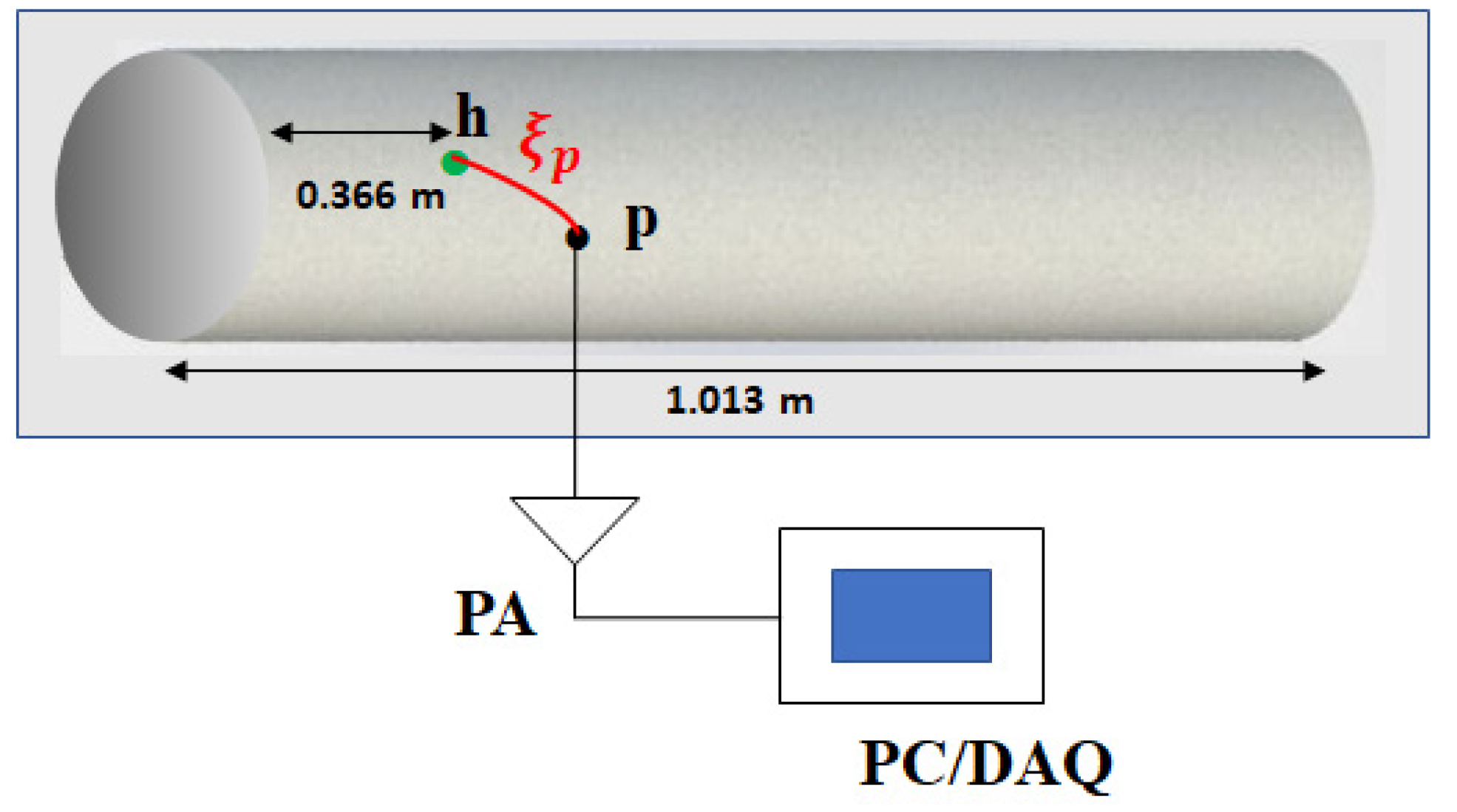
Figure 2.
(a) Angular dependence of the mean amplitudes (circles) and σs (bars) of signal obtained by an external excitation (1.000 Vpp and kHz) and the simulated displacements (lines) at different values of (1: 6.0, 2: 7.0, 3: 7.5, 4: 8.0, 5: 9.0), (b) axial dependence of the mean amplitudes of signal and the simulated displacement (line) with = 7.5.
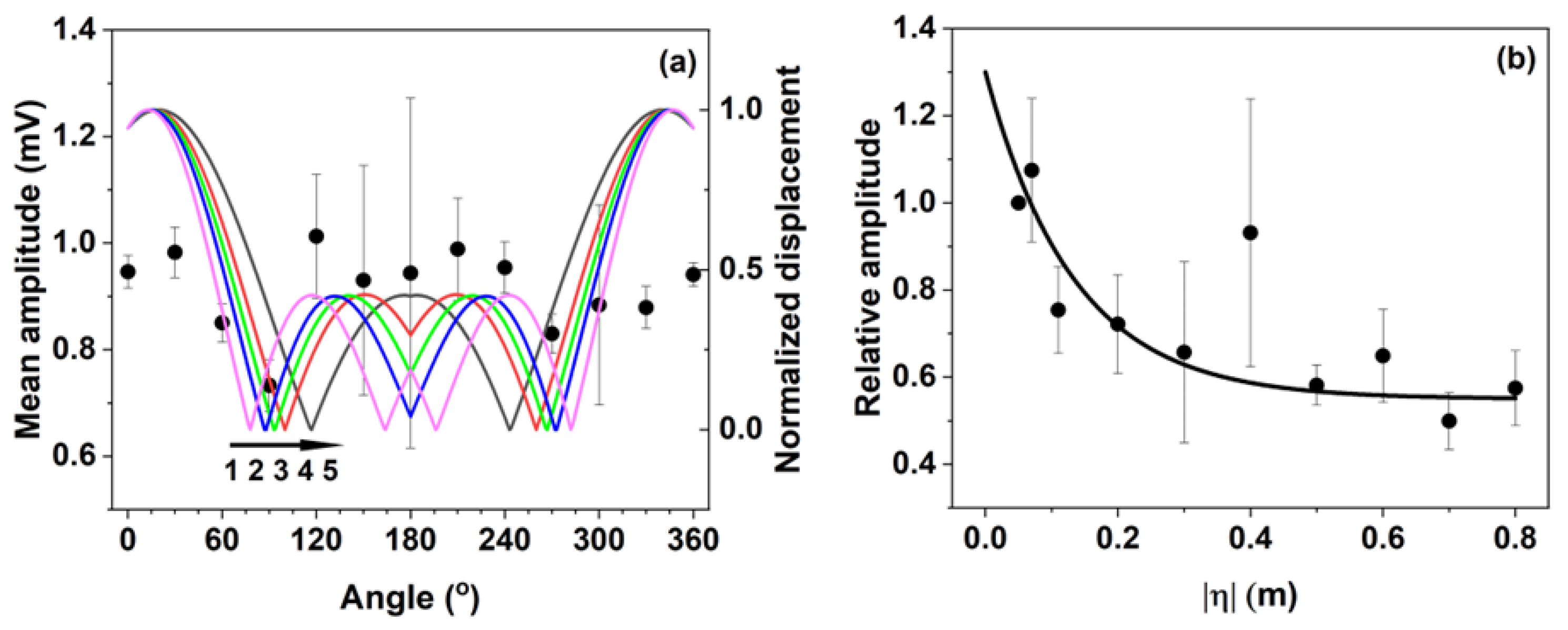
Figure 3.
(a–e) Observed mean maximum-amplitudes (circles) and σs (bars) obtained from five different hole diameters: (a) D0.2η10, (b) D0.3η10, (c) D0.5η10, (d) D0.8η10 and (e) D1.2η10 at = 2 bar (black), 3 bar (red) and 4 bar (green), and simulated amplitudes (lines), and (f) plot of mean amplitudes (circle) at ° vs. Reynolds number and the fit (line) by one-phase exponential growth.
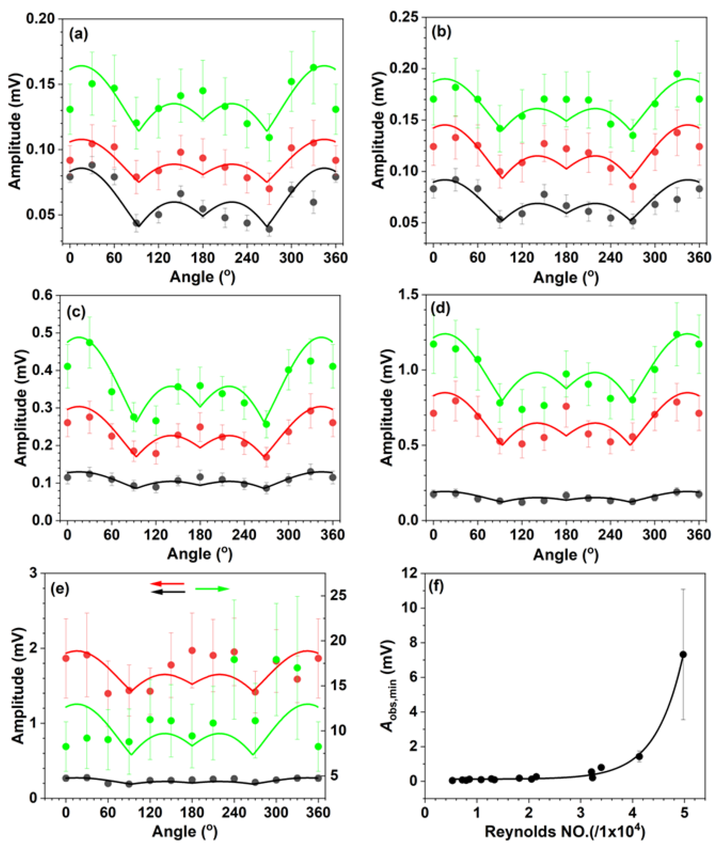
Figure 4.
Observed mean maximum-amplitudes (circles) and σs (bars) obtained from four different axial positions: (a) D0.2η3, (b) D0.2η30, (c) D0.2η50, and (d) D0.2η70 at = 2 bar (black), 3 bar (red) and 4 bar (green), and simulated amplitudes (lines).
Figure 4.
Observed mean maximum-amplitudes (circles) and σs (bars) obtained from four different axial positions: (a) D0.2η3, (b) D0.2η30, (c) D0.2η50, and (d) D0.2η70 at = 2 bar (black), 3 bar (red) and 4 bar (green), and simulated amplitudes (lines).
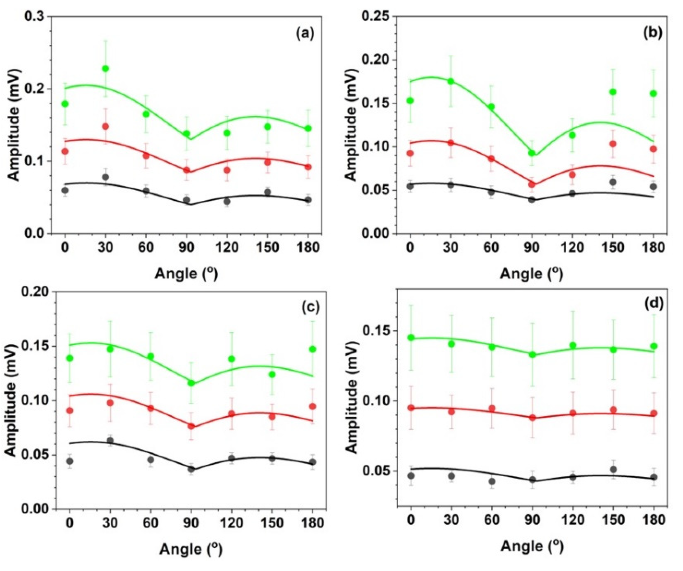
Figure 5.
(a–e) Observed mean maximum-amplitudes (circles) and σs (bars) obtained from five different hole diameters: (a) D0.2180, (b) D0.3180, (c) D0.5180, (d) D0.8180 and (e) D1.2180 at P = 2 bar (black), 3 bar (red) and 4 bar (green), and simulated amplitudes (lines), and (f) plot of values (circles) vs. Reynolds NO and the fit (line) by one-phase exponential growth.
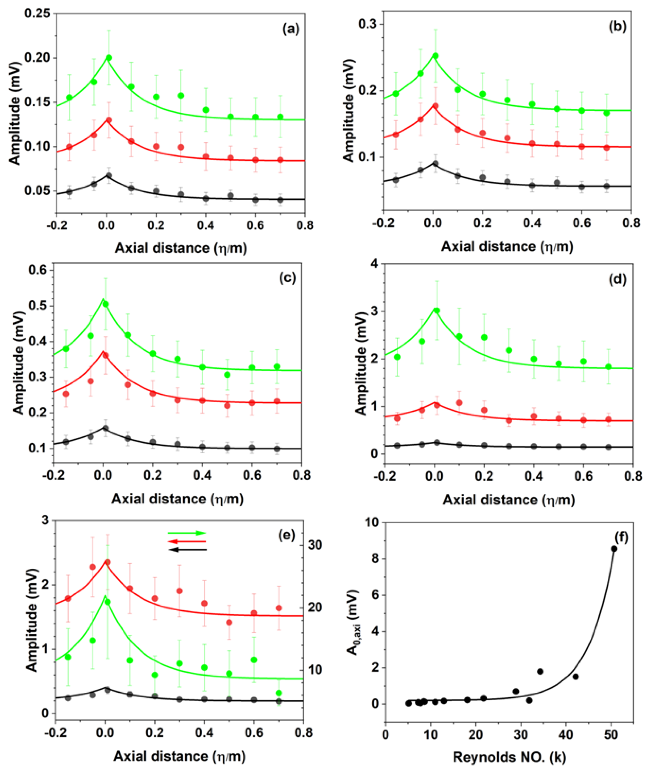
Figure 6.
Fitting the angular (a, c) and the axial (b, d) dependences of the observed mean maximum-amplitudes (circles) and σs (bars) obtained from the sensor array in Zone1 (a, b) and Zone2 (c, d) to the simulated values (solid lines) (three different gas pressures used).
Figure 6.
Fitting the angular (a, c) and the axial (b, d) dependences of the observed mean maximum-amplitudes (circles) and σs (bars) obtained from the sensor array in Zone1 (a, b) and Zone2 (c, d) to the simulated values (solid lines) (three different gas pressures used).
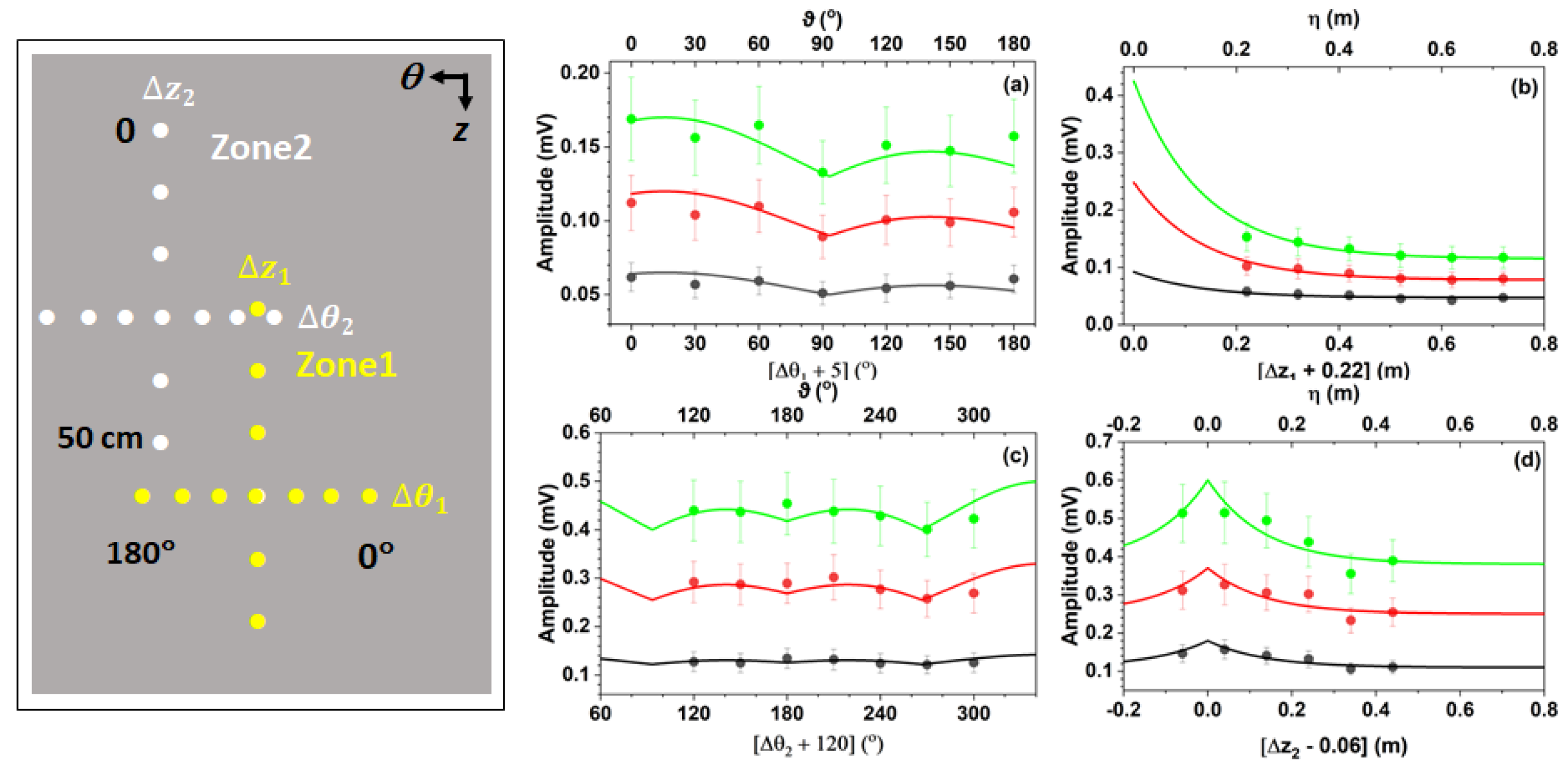

Table 1.
Material and geometric properties of the leak test cylinder, and molecular and thermal properties of the charged gas.
Table 1.
Material and geometric properties of the leak test cylinder, and molecular and thermal properties of the charged gas.
| Steel cylinder |
|---|
| m, m kg m-3, m m s-1, m s-1 |
| Stiffness parameters (kg m-1 ms-2) c11 = 208.6 × 10⁹, c22 = 208.6 × 10⁹, c33 = 208.6 × 10⁹, c12 = 146.5 × 10⁹, c13 = 146.5 × 10⁹, c23 = 146.5 × 10⁹ c44 = 126.9 × 10⁹, c55 = 126.9 × 10⁹, c66 = 126.9 × 10⁹ |
| Nitrogen gas (25°C, 1 bar)* |
| kg m-3 m2 s-1 |
Table 2.
Results for the localization of the leak source determined by fitting the observed signal amplitudes to the simulated values. The leak source locates at = 0° and .
Table 2.
Results for the localization of the leak source determined by fitting the observed signal amplitudes to the simulated values. The leak source locates at = 0° and .
| Array position |
P0 (bar) |
(error%) |
/mm (error%) |
Reynolds NO/k Theory/estimation |
|
|---|---|---|---|---|---|
| Zone1a | 2.07 3.06 3.97 |
-6.1° (1.7) -6.1° (1.7) -6.1° (1.7) |
5.0 (0.5) 5.0 (0.5) 5.0 (0.5) |
0.05/0.05 0.09/0.08 0.13/0.12 |
5.3/5.5-5.9 7.2/7.0-8.4 8.5/8.5-11.7 |
| Zone2b | 2.01 3.01 4.01 |
3.6° (1.0) 3.6° (1.0) 3.6° (1.0) |
7.0 (0.7) 7.0 (0.7) 7.0 (0.7) |
0.12/0.11 0.26/0.25 0.40/0.38 |
13.3/8.0-11.0 18.1/18.1-23.0 21.5/28.9 |
a,b Two different hole sizes were used: a; D0.2 and b; D0.5
Disclaimer/Publisher’s Note: The statements, opinions and data contained in all publications are solely those of the individual author(s) and contributor(s) and not of MDPI and/or the editor(s). MDPI and/or the editor(s) disclaim responsibility for any injury to people or property resulting from any ideas, methods, instructions or products referred to in the content. |
© 2025 by the authors. Licensee MDPI, Basel, Switzerland. This article is an open access article distributed under the terms and conditions of the Creative Commons Attribution (CC BY) license (https://creativecommons.org/licenses/by/4.0/).
Copyright: This open access article is published under a Creative Commons CC BY 4.0 license, which permit the free download, distribution, and reuse, provided that the author and preprint are cited in any reuse.


