
Submitted:
12 July 2025
Posted:
15 July 2025
You are already at the latest version
Abstract
In this paper, the author utilizes the frailty model to construct a new Archimedean copula. This copula depends on the transformed Median Based Unit Rayleigh (MBUR) distribution to an unbounded distribution defined on the interval from zero to infinity. The copula only models the positive dependency. In the paper, the joint PDF and CDF of the copula are derived for two bivariate distributions. The singularity of the copula is explained. The generator and inverse generator of the new copula are explored to depict the decreasing and convex nature of the generator. The Kendall tau measure of dependency is derived. For this copula, the lower and upper tail dependencies exist. The formula for each one is derived. Inference Function for Margin (IFM) is explored and utilized in real data analysis. This new copula is one of the parametric Archimedean copulas. Unfortunately, the Archimedean copulas are not widely used.
Keywords:
frailty model
; archimedean copula
; generator
; inverse generator
; MBUR distribution
; Inference Function for Margin
1. Introduction
A copula is a function mapping and satisfying the boundary condition in the form
of , the unit marginal conditions in the form of , and 2-increasing property that states,
then,
.
and for , hence satisfying Lipschitz condition that is .
Sklar (Sklar, 1973) showed that a copula exists for
any multivariate distribution, such that the joint distribution equals the
copula applied to the marginal. In other words, Let X and Y be random
variables with joint distribution and marginal distribution functions and , respectively. Then there is a uniquely
determined copula, C, on the , such that for So copulas connect joint distributions functions
to their margins. They are crucial for constructing bivariate and multivariate
distributions because they are a statistical method for studying scale-free
measures of dependence.
Definition1 (Sklar’s theorem 1):
For any bivariate distribution function H with marginal and , there exists a copula such that
If H is continuous, then the copula C is unique.
Otherwise, it is uniquely determined on the . The converse is also true, for any copula and
univariate distribution functions and , the function is a bivariate distribution function with margins
and .
Definition 2 : A bivariate Archimedean
copula can be written in the form of with marginal and , where is the generator function being continuous,
strictly decreasing and convex function mapping onto , in other words , ( decreasing) and ( convex) , , and
Definition 3: a bivariate copula has which is the joint PDF of the copula.
So the copula links the marginal distributions
through the dependency parameter.
The singular part of the copula is defined by (Genest
& Mackay, 1986) in the following Theorem, the ratio between the generator
and the first derivative of the generator evaluated at zero does not equal
zero.
Theorem: the distribution generated by has a singular component iff in that case, with probability = In the last few years many models have been
proposed for copulas. The applications of copulas are too plentiful to list so
further improvements of copulas are encouraged to be further advanced. The
applied applications rely mainly on the parametric models for copulas in
comparison to the semi-parametric and non-parametric model for copulas which
have limited applied implementations in real life.
Many eminent scientists and authors had in depth
papers discussing the estimation methods, simulation, probabilistic
interpretations, and analytical properties. Many problems face the statistical
scientific community and in need for solutions. (Nadarajah et al., 2018)
mentioned some of these problems like estimation of copula under
misspecification, copula density estimation , Bayesian copula, change point
estimation of copulas, efficient estimation and simulation algorithms,
characterization of copulas, selection criteria between two or more copulas,
time series models constructed on copulas, bounds for copulas, copula
calibration, transformations to enhance fits of copulas, extreme value manners
of bivariate and multivariate copulas, compatibility of copulas, additional
measures of asymmetry for bivariate and multivariate copulas, extra tests for
symmetry for bivariate and multivariate copulas, , time varying copulas, space
changing copulas and copulas fluctuating with sense of both time and space.
Many books had been written by pioneer and
innovator scientists in the field of copulas like books written by (Drouet-Mari
& Kotz, 2001), (Cuadras et al., 2002), (Cherubini et al., 2004), (Genest,
2005a), (Genest, 2005b), (Nelson, 2006), (McNeil et al., 2005), (Alsina et al.,
2006), (Mai & Scherer, 2014), (Durante & Sempi, 2015), (Salvadori et
al., 2007), (Malevergne & Sornette, 2006), (Schweizer
& Sklar, 2005), (Jaworski et al., 2010),(Jaworski et al., 2013), (Jaworski
et al., 2010; Joe, 2014), (Joe, 1997)and many others. Numerous papers
had been published by many prominent scientists like (Nelsen,
2002), (Embrechts et al., 2003), (Manner & Reznikova, 2012), (Patton, 2012),(Genest
et al., 2009),(Schweizer, 1991), (Kolev et al., 2006), (Kolev & Paiva,
2009), and (Frees & Valdez, 1998).
The copula can be grouped into five subgroups which
are the Archimedean copulas, the elliptical copulas, the
Eyraud-Farlie-Gumbel-Morgenstern (EFGM) copula, extreme value copulas, and
other copulas. Each of these subgroups includes more copulas. For more
details, the reader can be referred to the paper of (Nadarajah et al., 2018)
and references therein.
The simplest copula is the product copula or the
independence copula .It is for two independent random variables with .The other two very essential dependencies between
two variables are the perfect positive and the perfect negative dependencies.
These can be expressed by copulas. For the positive state, this yields . Hence, for random variables X and Y with
distributions , and the joint distribution ,and because the copula is symmetric, the random
variable X is an increasing function of Y and vice versa. The converse, with
decreasing instead of increasing holds true for the joint distribution function
with . This one is also a copula. These boundaries are
themselves copulas and they are called Frechet-Hoeffding upper and lower bound
respectively. As long as both and are not differentiable in u and v, they have no
density functions. Joe (Joe, 1990), (Joe & Hu, 1996), (Joe, 1993) developed
copulas that allow for positive dependency only. These copulas are recently
used in portfolio risk analysis with Asian equity markets (Ozun & Cifter,
2007).
This paper is structured in 9 sections. Section 1 discusses the methodology of
derivation. section 2 illustrates the generator and its properties. Section 3 explores the inverse generator and
its properties. Section 4 explains the
Kendal Tau measure of dependency. Section 5
enlightens how the copula can model both lower and upper tail dependencies. Section 6 elucidates methods of estimation. Section 7 demonstrates real data analysis. Section 8 comprehends the conclusion. Section 9 states future works.
2. Methodology of Derivation
This copula depends on the frailty method for
generating the copula. Assuming two individuals have survival time distributed
as exponential and .They have exponential baseline hazard function
with . The survival function is shown in equation (1)
and the hazard function in equation (2)
The Cox proportional hazard model uses the hazard
function as shown in equation (3)
where the Z are the explanatory variables in
survival analysis and b(t) is the baseline hazard function. And B is the vector
of regression coefficients. It is proportional because all information is
contained in the multiplicative factor , this is called the frailty model when some
explanatory variables (Z) and hence the factor are unobserved. And the factor is called the frailty parameter. is the result of integration and exponentiation of
the negative hazard in equation (2) or hazard in equation(3). For exponential random variable
the hazard is expressed in terms of explanatory variables, for example 2
variables as where and assume.
where is the baseline hazard, to sum up assuming .
The marginal distribution for a single life time T
is obtained by taking expectation over the potential values of that is , assuming the is the PDF of the frailty variable so
Let y be a random variable distributed as Median
Based Unit Rayleigh (MBUR) (Attia, M.I., 2024), transform this variable to be
defined on the interval from zero to infinity as shown below. The PDF of the
Median Based Unit Rayleigh (MBUR) is shown in equation (4)
The transformation in equation (5.A) and the
Jacobian in equation (5.B) will be applied to the above PDF:
Replace equation (5) into equation (4) as shown in
equation (6):
Now this w is the frailty variable which is distributed as unbounded MBUR defined on
the interval . Now take the conditional expectation of the
survival function of the time distributed as exponential random variable with
hazard rate equal one (scale parameter or lambda=1) given the frailty variable
as shown in equation (7)
We can think of this expectation as a function of
the frailty variable, it is averaging the probability to survive beyond
specific time given that frailty. It is the expectation of a function of the
frailty not the variable frailty itself so this function which is the baseline
survival function should be multiplied by the PDF of the frailty variable. This
way the frailty variable is integrated out. So this expectation is considered
as the joint CDF of the two random variables T1 and T2. How to get this time?
By inverting this expectation as shown in equation (8). Let us call this
expectation u then solving second degree polynomial to get its root.
3. The Generator
In equation (8); the generator is not defined in
term of the dependency parameter so re-parameterization of the generator
yielded a generator with a dependency parameter. The author added dependency
parameter and remove the denominator as shown in equation (9), is the marginal CDF.
This (t) is the generator and (u) is the inverse
generator. So the time (t) is a function of (u)
Preposition 1: the generator shown in
equation (9) , can be considered as a generator for this new
Archimedean copula.
Proof : The generator in equation (9)
fulfills the sufficient conditions of a generator.
(1)
(2)
(3)
This ensures that the generator is a decreasing
function in u .
(4)
This ensures that the generator is a convex
function at For bivariate distribution with uniform marginal
CDF (u) and (v), the generators are shown in equations (10-12)
&&
4. The Inverse Generator
To get the inverse generator of this modified
generator, the author inverts this (t) as shown in equation (13), as long as t
equals:
Recall that and a valid bivariate Archimedean copula can be
expressed as
Proposition 2: The copula expressed in
equation (13) can be assumed to be a valid copula if it fulfills the boundary
conditions, the marginal uniformity and 2- increasing conditions. And these are
the necessary conditions that should be fulfilled by the inverse generator.
Proof:
, boundary conditions are fulfilled
, the marginal uniformity, when u=1
The same is true for v , if v=1 so
Proposition 3: This is a valid copula as it
is 2-increasing, i.e. , as shown in equation (14)
Proof:
Let
satisfying the 2-increasing condition.
This density function in equation 14 integrates to
one using MCMC simulation from zero to one.
Proposition 4: This copula is absolutely
continuous copula and it has no singular part.
Proof: to test for singularity: as shown in equation (15). If this limit is zero
so the copula has no singular part.
As long as this limit is zero at u=0 so the copula
has no singular part and it is absolutely continuous copula.
5. Kendall Tau Measure of Dependency
Proposition 5: Kendall tau for this copula
is in equation (16)
Proof:
Figures (1-30)
illustrate the joint PDF, the joint CDF and the related generator for the
copula with different values of dependency parameter.
6. Tail Dependency
Preposition 6: The upper and lower tail
dependency for this copula exist as shown in equation (17-18).
Proof: for the upper tail dependency
where
For lower tail dependency:
But the lower tail dependency coefficient is
between 0 and 1 and it cannot exceed the 1, so it is calculated as
So the upper tail dependence coefficient for of this copula is , also the copula has a lower tail dependency not
exceeding the one for . The , when dependency parameter approaches 0. While , when this parameter is 1. The exists as shown in equation (18) and cannot exceed
one. Also the following equations (19-20) support these findings.
Upper tail dependency
As long as u is small
This upper tail dependency cannot exceed one
especially at very small values of the dependency parameter.
Lower tail dependency:
This lower tail dependency cannot exceed one
especially at very small values of the dependency parameter.
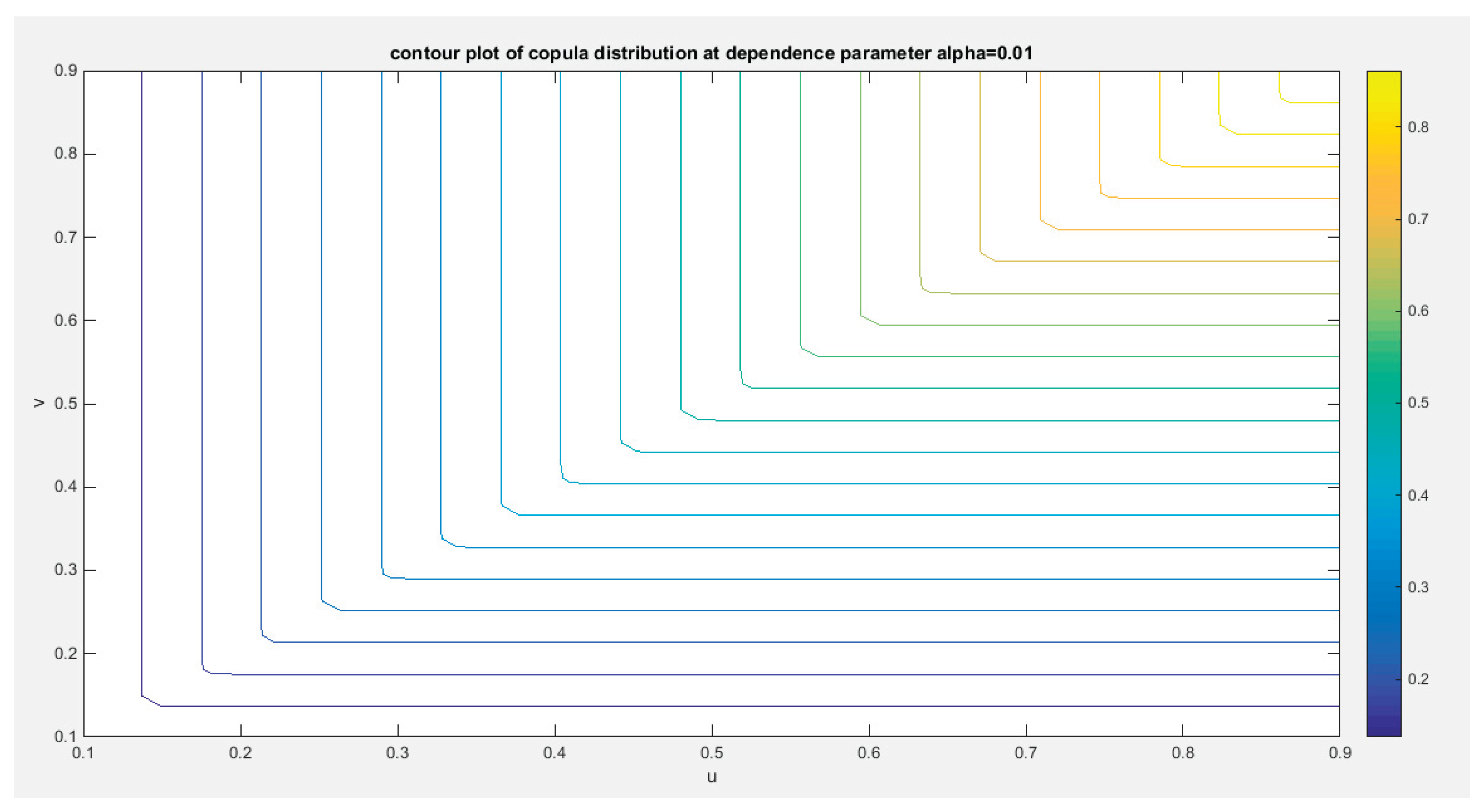
Figures (1-2)
illustrate the contour plot and the surface of the copula density and
distribution with different values of the dependency parameter.
Figure 1.
shows copula density surface with dependency parameter 0.1.
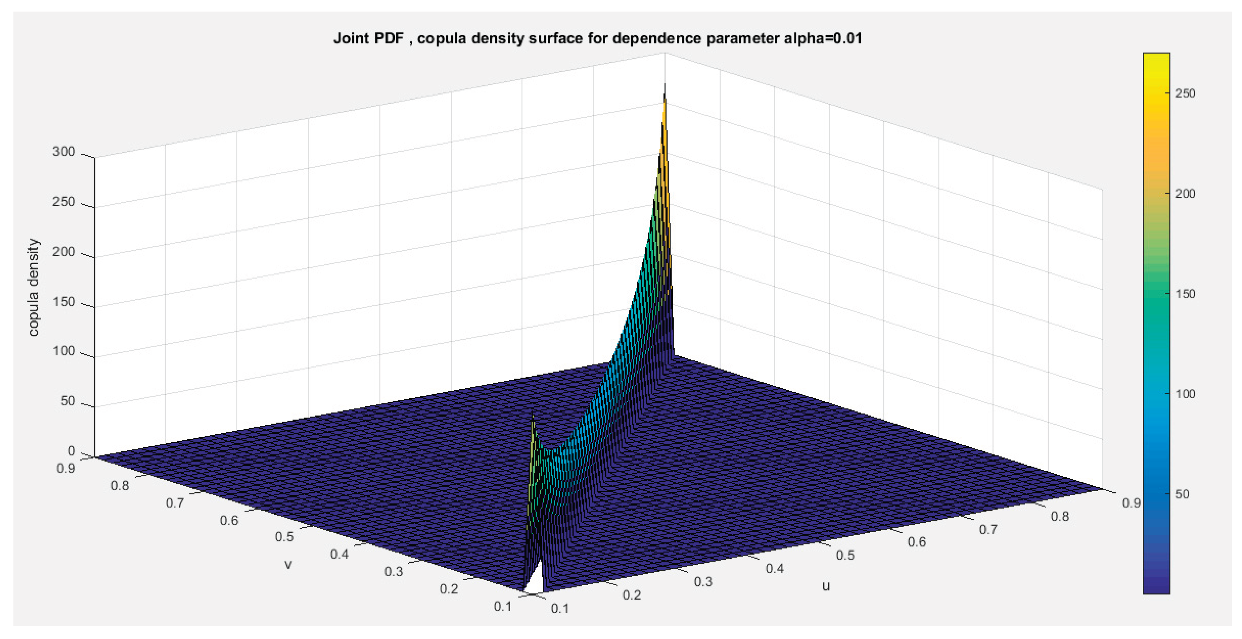
Figure 2.
shows the contour plot of the copula distribution with dependency parameter 0.01.
7. Methods of Estimation
(Weiß, 2011), (Chen, 2007), and (Tsukahara, 2005)
provided a comprehensive overview of various estimation methods, including the
following:
7.1. Maximum Likelihood Estimation (MLE)
The process involves a single step in which all
parameters—both marginal and copula—are estimated for the complete joint
density function. This is accomplished by taking the log-likelihood of the full
joint function, differentiating it with respect to each of the marginal
parameters and the copula parameter, then setting the resulting equations equal
to zero. Finally, the system of equations is solved numerically.
7.2. Inference Function of Margins (IFM)
In the context of bivariate copula-based models,
estimating all model parameters simultaneously using maximum likelihood can be
computationally challenging (Al Turk et al., 2017). To address this issue, a
two-stage estimation procedure has been suggested by researchers such as (Joe,
2005) and (Xu, 2009). n the first stage of this approach, the marginal
parameters are estimated independently using maximum likelihood, as detailed in
equation (21). Here, "s" represents the score function or gradient,
which plays a crucial role in the estimation process.
By accurately estimating the marginal parameter,
you unlock the potential to derive the marginal cumulative distribution
function (CDF) for each variable, as demonstrated in equation (22). This
pivotal step not only deepens your understanding of each variable's behavior
but also equips you with powerful insights that can significantly enhance your
analysis. Embrace this method to elevate the sophistication of your findings!
In the second stage of the analysis, we focus on
maximizing the likelihood of the dependence parameters while keeping the
marginal parameters fixed, as determined in the first stage. This process
involves calculating the log-likelihood of the copula density, which is
represented in equation (23). To further this analysis, we then differentiate
the log-likelihood with respect to the copula dependency parameter, as outlined
in equation (24).
In this paper, the author used IFM.
Taking the first derivative of the log-likelihood
of equation (14) with respect to copula parameter as described below: the
copula density can be written as so
This t4 can be written as and
let’s call
Applying Quasi-Newton method
where , and can approximate the variance of the dependency parameter estimator.
Each marginal parameter possesses its own variance, which is determined in the first stage of the (IFM) approach. In the second stage, these parameters are treated as fixed, which means they do not directly influence the variance of the estimated dependency parameter. While the variance of the copula parameter derived from the second stage remains valid under the IFM approach, it consistently underestimates the total uncertainty by neglecting the variability associated with the estimation of marginal parameters. To effectively propagate uncertainty from the first stage to the second stage, it is imperative to employ the Godambe information matrix (commonly referred to as the sandwich estimator), as articulated (Godambe, 1991). This rigorous approach facilitates the calculation of the joint variance-covariance matrix for all parameters, encompassing both marginal and copula parameters. The sandwich estimator is a robust variance estimator, crucial for obtaining the asymptotic variance of parameter estimates, particularly when the likelihood function is estimated in multiple stages or is mis-specified due to failure to utilize the full joint likelihood. The variance is defined by the following equation (25):
The second stage involves estimating the copula dependency parameter using the pseudo likelihood function as shown in equation (26-28) and maximizing this function.
where S is the outer product of the gradient of parameter estimator (marginal and copula) or the score function as shown in equation (29).
is the inverse of the negative of the expectation of the information matrix, in other words, the variance of the parameter estimator (marginal and copula). It is a diagonal matrix. , the inverse of this H or inverse of this I is the variance of marginal parameter estimators in the first stage and the variance of the copula estimator in the second stage. So let’s call this inverse the A matrix, so the sandwich estimator can be expressed as shown in equations (30-31)
This variance covariance matrix captures the covariance between the marginal and the copula parameter estimators which are not captured in the naive block-separated IFM variances.
7.3. Semiparametric Method (SP)
The third method introduced by (Kim et al., 2007) is the estimation by semiparametric method (SP This process is divided into two stages, similar to (IFM). In the first stage, the variables are transformed into their marginal empirical cumulative distribution functions (eCDF). Essentially, this involves converting the observations into pseudo-observations by applying the empirical distribution function to each marginal distribution, as demonstrated in equation (32).
The second stage involves estimating the copula dependency parameter using the pseudo likelihood function as shown in equation (33-34) and maximizing this function.
8. Real Data Analysis
8.1. Data Description
The OECD data platform, offered by the Organization for Economic Cooperation and Development (OECD), serves as a valuable resource by collecting comprehensive data across diverse economic, social, and environmental sectors, including the economy, health, trade, education, labor, innovation, and development. This platform presents a wide array of indicators that effectively describe these aspects. In this analysis, the focus will be on two key indicators to examine their interrelationships and explore how new copulas can be utilized to model these dependencies. The selected indicators include: ‘feeling safe walking alone at night’ and ‘the quality of support networks’ coded (1) & (2) respectively in Table (1). The data collection encompasses 41 countries, providing a robust foundation for our insights and conclusions. The data can be found on the following site: https://stats.oecd.org/index.aspx?DataSetCode=BLI .
The indicators ( let’s call it the y variable) in Table (1) are distributed as Median Based Unit Rayleigh (MBUR) previously discussed by Iman Attia (Attia, 2024) with the following PDF in equation (35), CDF in equation (36), and, quantile function in equation (37):

Table 1.
the 2 indicators in OECD data and the 2 indicators. 1 for ‘feeling safe walking alone’ and 2 for ‘Quality of support network’.
Table 1.
the 2 indicators in OECD data and the 2 indicators. 1 for ‘feeling safe walking alone’ and 2 for ‘Quality of support network’.
| Australia | Austria | Belgium | Canada | Chile | Colombia | Costa Rica | Czechia | |
| 1 | 0.67 | 0.86 | 0.56 | 0.78 | 0.41 | 0.50 | 0.47 | 0.77 |
| 2 | 0.93 | 0.92 | 0.90 | 0.93 | 0.88 | 0.80 | 0.92 | 0.96 |
| Denmark | Estonia | Finland | France | Germany | Greece | Hungary | Iceland | |
| 1 | 0.85 | 0.79 | 0.88 | 0.74 | 0.76 | 0.69 | 0.74 | 0.85 |
| 2 | 0.95 | 0.95 | 0.96 | 0.94 | 0.90 | 0.78 | 0.94 | 0.98 |
| Ireland | Israel | Italy | Japan | Korea | Latvia | Lithuania | Luxembourg | |
| 1 | 0.76 | 0.80 | 0.73 | 0.77 | 0.82 | 0.72 | 0.62 | 0.87 |
| 2 | 0.96 | 0.95 | 0.89 | 0.89 | 0.80 | 0.92 | 0.89 | 0.91 |
| Mexico | Netherlands | New Zealand | Norway | Poland | Portugal | Slovak Republic | Slovenia | |
| 1 | 0.42 | 0.83 | 0.66 | 0.93 | 0.71 | 0.83 | 0.76 | 0.91 |
| 2 | 0.77 | 0.94 | 0.95 | 0.96 | 0.94 | 0.87 | 0.95 | 0.95 |
| Spain | Sweden | Switzerland | Turkey | United Kingdom | United States | Brazil | Russia | |
| 1 | 0.80 | 0.79 | 0.86 | 0.59 | 0.78 | 0.78 | 0.45 | 0.64 |
| 2 | 0.93 | 0.94 | 0.94 | 0.85 | 0.93 | 0.94 | 0.83 | 0.89 |
| South Africa | ||||||||
| 1 | 0.40 | |||||||
| 2 | 0.89 |
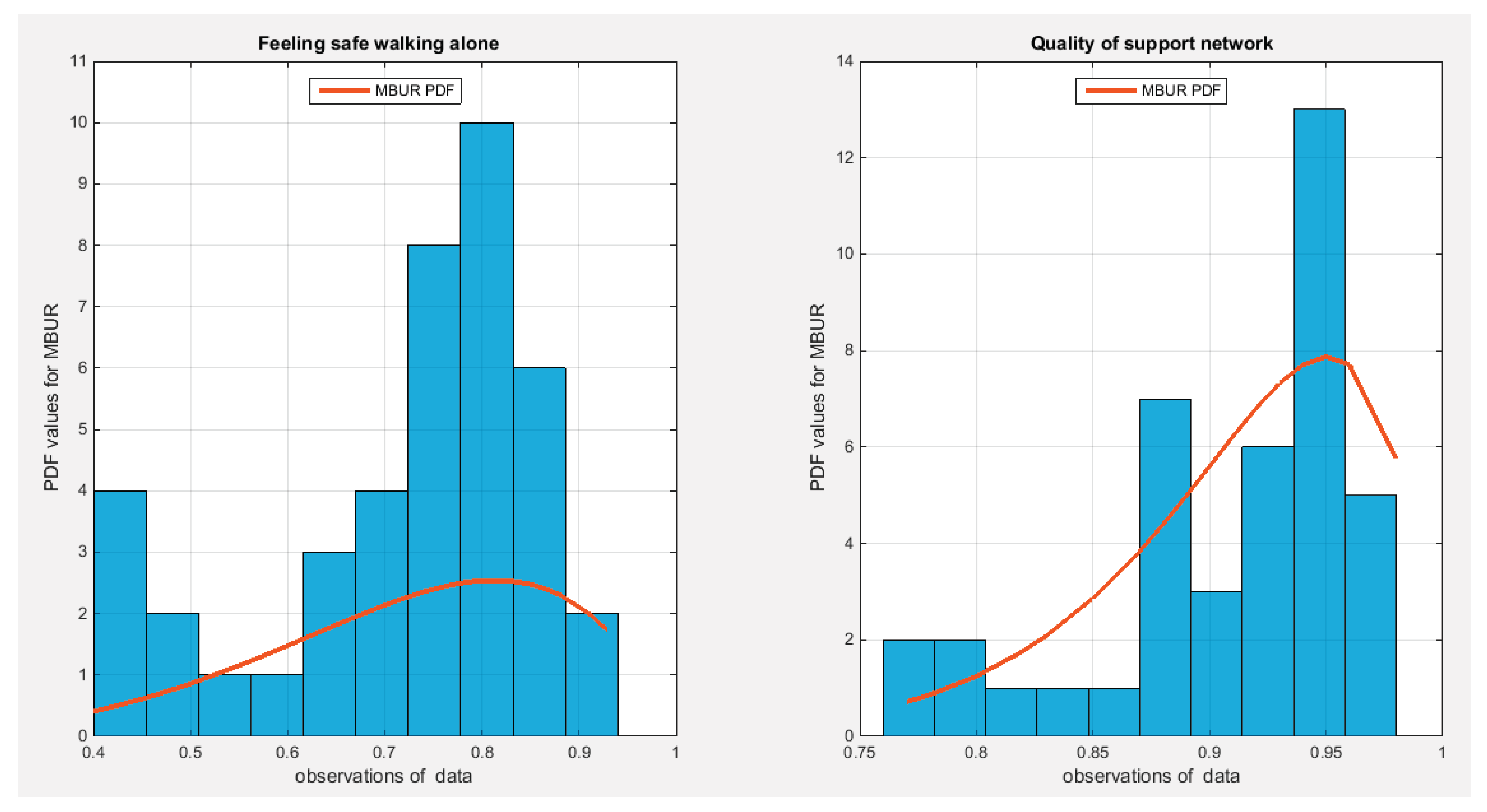
The indicator of ‘feeling safe walking alone’ measures the percentage of people who report feeling safe when walking alone in their local area after dark. The ‘quality of support network’ indicator measures the accessibility and trustworthiness of social support for individuals and it is explicated as the percentage of population with social support who described having someone they can depend on for support when they need it. Table (2) shows the descriptive statistics of the 2 indicators. Table (3) shows the empirical Kendall tau coefficient and its associated p-value. Figure (3) shows the boxplot for each indicator. Figure (4) show the scatter plot of the dependent indicators. Each indicator fits the Median Based Unit Rayleigh Distribution (MBUR). Table (4) shows the statistical validity indices for each indicator. Figure (5) shows the histogram and the fitted MBUR curve for each indicator.
Table 2.
descriptive statistics for the 2 indicators:.
| Indicator | Min | Mean | Standard Deviation | Skewness | Kurtosis | 25percentile | 50percentile | 75percentile | Max |
| Feeling safe walking alone | 0.4 | 0.7207 | 0.143 | -0.9486 | 3.0353 | 0.655 | 0.76 | 0.8225 | 0.93 |
| Quality of support network | 0.77 | 0.9078 | 0.0538 | -1.176 | 3.5406 | 0.89 | 0.93 | 0.95 | 0.98 |
Table 3.
empirical Kendall tau coefficient of the 2 indicators:.
| Feeling Safe Walking Alone | Quality of Support Network | |
| Feeling safe walking alone | 1 |
0.4344 (0.0001) |
| Quality of support network |
0.4344 (0.0001) |
1 |
Table 4.
statistical validity indices of the distributional fit (MBUR) of the 2 indicators:.
| Indicator | Estimated Theta | variance | AIC | CAIC | BIC | HQIC | KS-test | Ho | p-Value of KS-test |
| Feeling safe walking alone | 0.6494 | 0.0013 | -47.1347 | -47.0321 | -45.4211 | -46.5107 | 0.1206 | Fail to reject | 0.5492 |
| Quality pf support network | 0.3444 | 0.00037494 | -131.6505 | -131.6505 | -131.5479 | -131.0265 | 0.1806 | Fail to reject | 0.1217 |
Figure 3.
shows the Boxplot for each indicator. They show similar pattern of skewness (left sides skewness). The quality of support network variable exhibits more skewness than the feeling safe walking alone variable.
Figure 3.
shows the Boxplot for each indicator. They show similar pattern of skewness (left sides skewness). The quality of support network variable exhibits more skewness than the feeling safe walking alone variable.
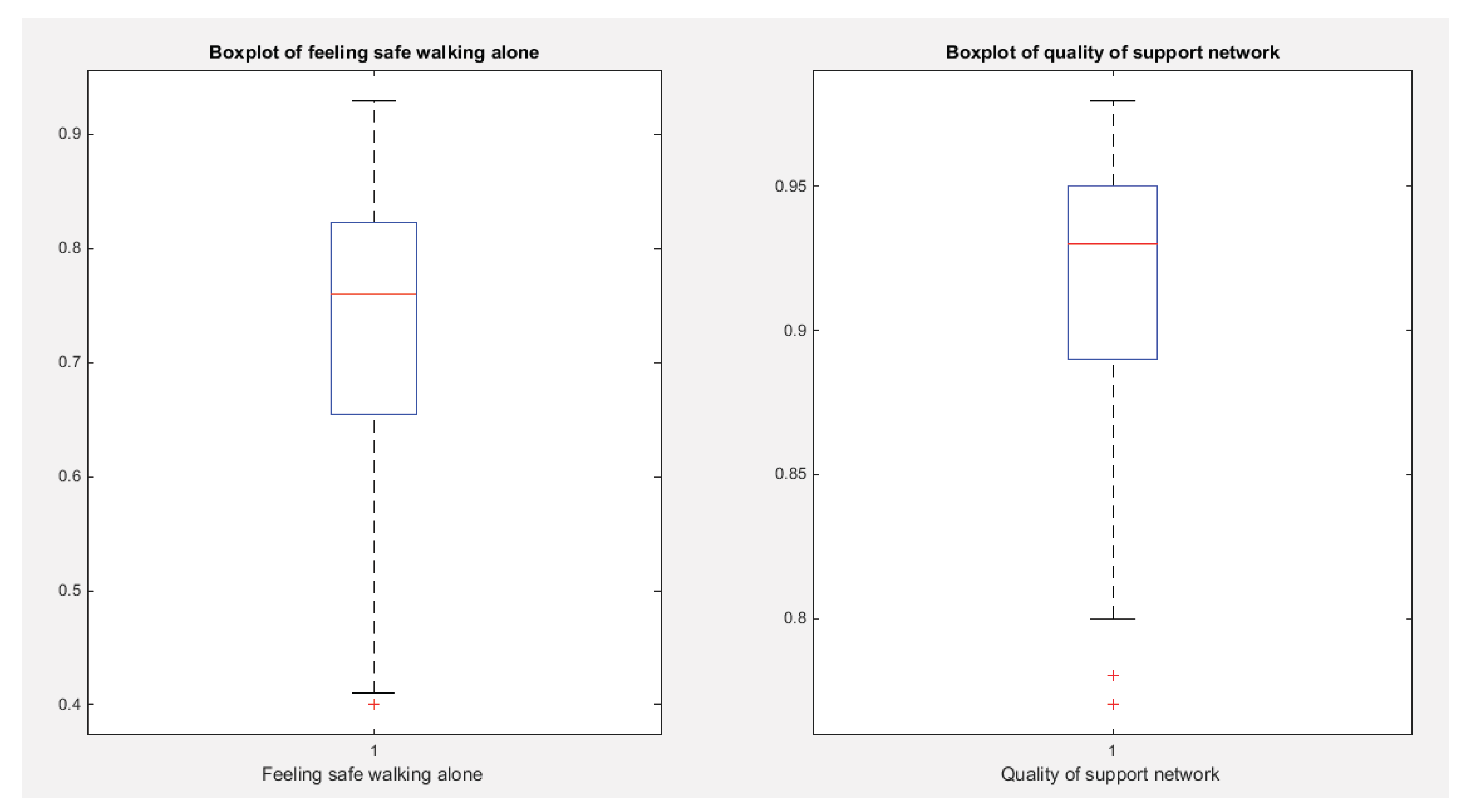
Figure 4.
shows the scatter plot of the variable feeling safe walking alone vs the variable of the quality of support network. The data are concentrated on the right upper corner of the graph.
Figure 4.
shows the scatter plot of the variable feeling safe walking alone vs the variable of the quality of support network. The data are concentrated on the right upper corner of the graph.
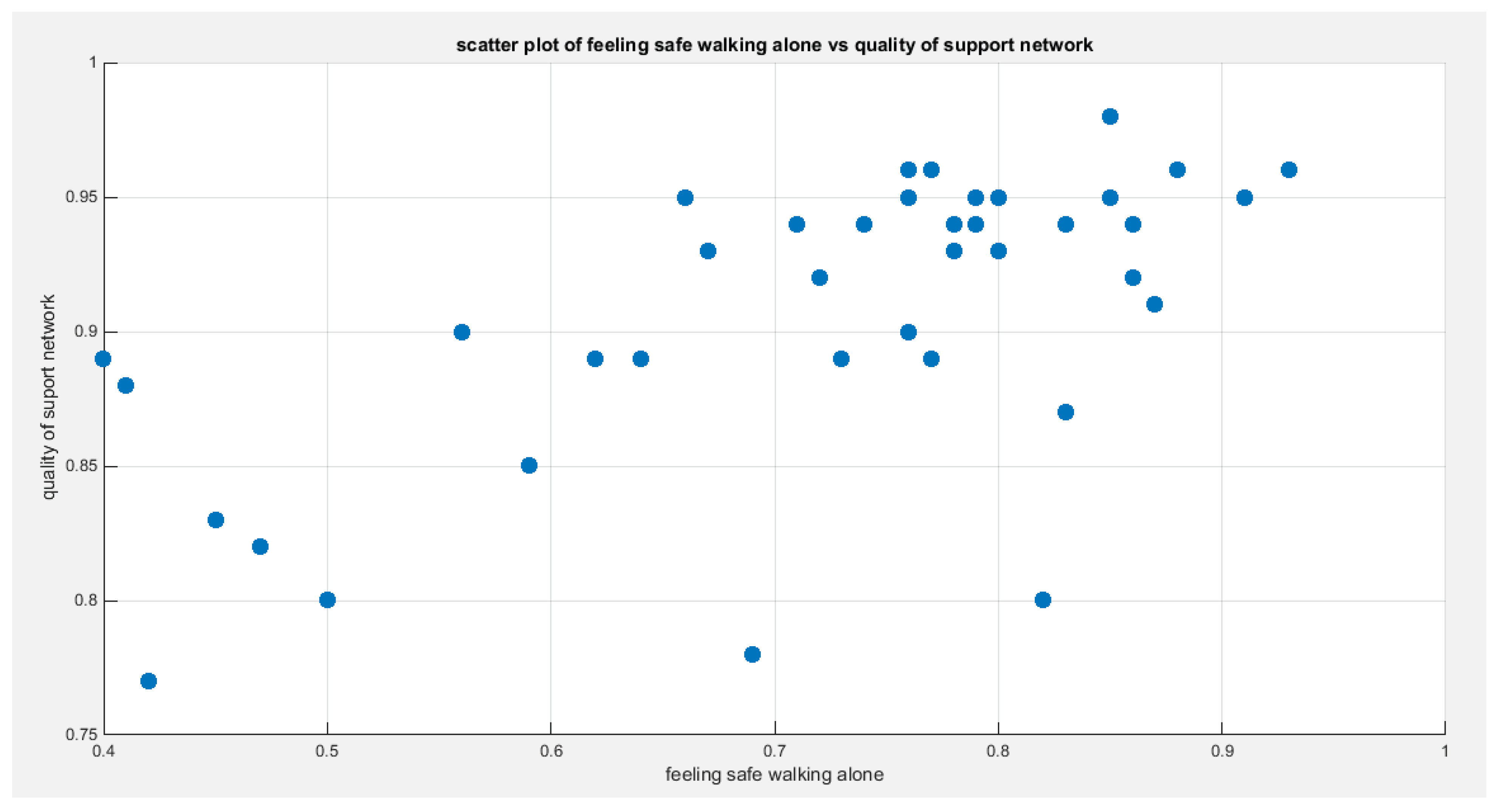
Figure 5.
shows the histogram of the two indicators which exhibit left sided skewness. The graph also shows the fitted MBUR curve for each indicator. The two indicators more or less have near similar kurtosis but the second one is more left skewed than the first. Copula that can fit symmetrical dependency can model dependency between such variables.
8.2. Procedure of Analysis (IFM)
After running the inference function for margins (IFM) and estimating the marginal parameter for each pair of variables then fitting each copula to estimate its parameter. Goodness of Fit tests are conducted to assess the dependence relationship for each pair of the variables.
The steps of analysis are as follows:
- Estimate the marginal parameters for each variable.
- Use the IFM procedure to estimate the dependency parameter of the proposed copula model.
- Obtain the theoretical tau from the specific relation between dependency parameter and the Kendall tau for the copula.
- Obtain the Cramer Von Mises test from this estimation process and call it CVMdata that will be compared to CVMsamples
- Run sampling technique like Metropolis Hasting (MH) procedure to test the null hypothesis using the estimated dependency parameter and both the estimated marginal parameters.
- Construct sampling distribution for the estimated-thetasamples , theoretical-tausamples , and CVMsamples .
For each of the sample generated by MH using the estimated dependency parameter and the estimated marginal parameters, they will be transformed back into variables using the specific quantiles. These variables will be subjected to the IFM procedure; first estimate the marginal parameters then using the estimated marginal CDF for each variable to estimate the dependency parameter, in other words, repeat steps (1 to 4) for each sample so you can be able to construct the sampling distribution, hence, constructing the confidence interval for each of the statistical indices. denotes theta estimated from the data.
The null hypothesis for the dependency parameter is: The alternative hypothesis for the dependency parameter is: The null hypothesis for the Kendall tau coefficient is: The alternative hypothesis for the Kendall tau coefficient is: The null hypothesis for the CVM is: The alternative hypothesis for the CVM is: Model the dependency between the ‘feeling safe walking alone’ and ‘Quality support network’: The empirical tau equals 0.4344 while the theoretical tau is 0.5428 with difference value of 0.1084. The estimated dependency parameter, theta , is 0.5714 with estimated variance of 0.0066. The Cramer Von Mises test (CVM) is 0.1948. The null hypothesis for dependency was tested by conducting resampling using the Metropolis Hasting algorithm of MCMC procedure. The proposed null hypothesis was that the dependency parameter equals the estimated theta against the alternative hypothesis that the population dependency parameter does not equal the estimated theta. Also the null hypothesis for the population Kendall tau coefficient being equal to the theoretical tau against the alternative hypothesis of not being equal to it was tested. The null hypothesis for the CVM proposing that the sampling CVM equals observed CVM obtained from the estimation procedure was investigated. The sampling distribution of each of the previously mentioned indices, thetas, tau and CVM is shown in Figures (6-8). For each figure, the descriptive statistics indices are shown. From the figures the indices are placed within the acceptance zone between the 2.5th and 97.5th quantiles. So the null hypotheses fail to be rejected. The copula fits the data well. And the dependence parameter models, within the context of the copula, the relation between the two variables. The confidence interval (CI) for the estimated dependence parameter is (0.3952, 0.7034), for the theoretical tau; it is (0.4373, 0.6839), and for CVM; it is (0.0303, 0.2417).
According to the sandwich variance the variance covariance matrix for this model is:
The validity indices for the second stage are:
The validity indices for the whole model is the summation of these indices for marginal (first stage) and copula (second stage):
Theoretical upper tail coefficient is 0.514. At quantile 0.7; the empirical upper tail coefficient in the direction of the ‘feeling safe walking alone’ variable is 0.5 (5 points showing joint match out of 10 points in the upper tail at this threshold, 0.7) and in the direction of the ‘Quality support network’ variable is 0.4545 (5 points showing joint match out of 11 points in the upper tail at this threshold, 0.7) while the confidence interval of the empirical distribution obtained from bootstrap sampling under the null hypothesis in both directions is [0.3 ,0.8889]. This is expected because of the small sample size and left skewness of data.
Theoretical lower tail coefficient is 0.4529. At quantile 0.1; the empirical lower tail coefficient in the direction of the ‘feeling safe walking alone’ variable is 0.5 (3 points showing joint match out of 6 points in the lower tail at this threshold, 0.1) and in the direction of the ‘Quality support network’ variable is 0.6 (3 points showing joint match out of 5 points in the lower tail at this threshold, 0.1) while the confidence interval of the empirical distribution obtained from bootstrap sampling under the null hypothesis in both directions is [0 ,1]. This is expected because of the small sample size and left skewness of data.
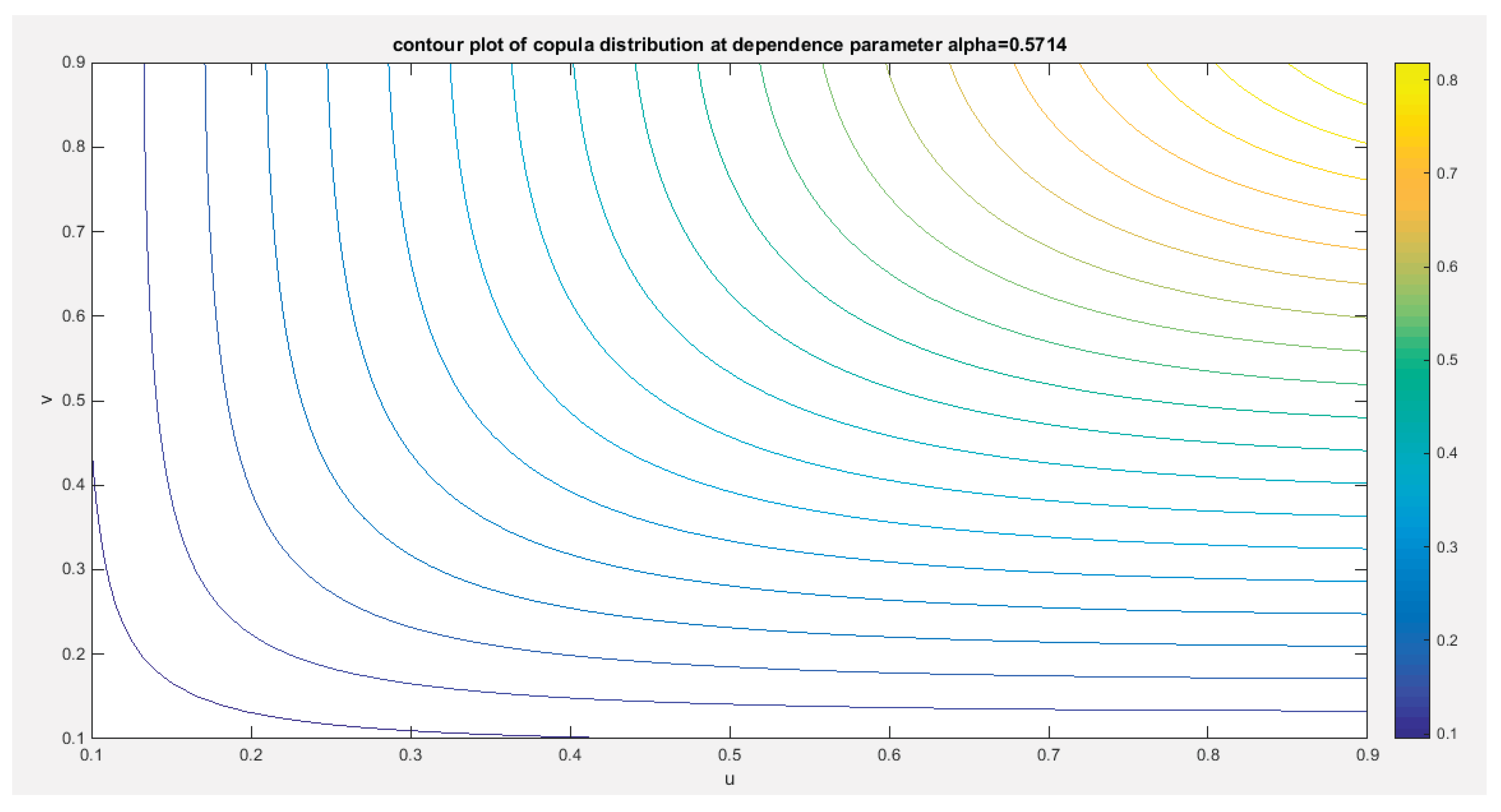
Figure 9 shows the P-P plot of the empirical vs the theoretical copula. Figure 10-12 show the surface of the copula density, the contour plot of the copula density, and the contour plot of the copula distribution at the estimated dependency parameter.
Figure 6.
shows the sampling distribution of the CVM. The CVMdata is 0.1948 and it lies between the 2.5th and the 97.5th quantiles so null hypothesis is failed to be rejected and the copula fits the data well. The p-value (probability of values less than or equal to 0.1948) is 0.938, in other words, this 0.1948 does not lay in either of the tail region of rejection. .
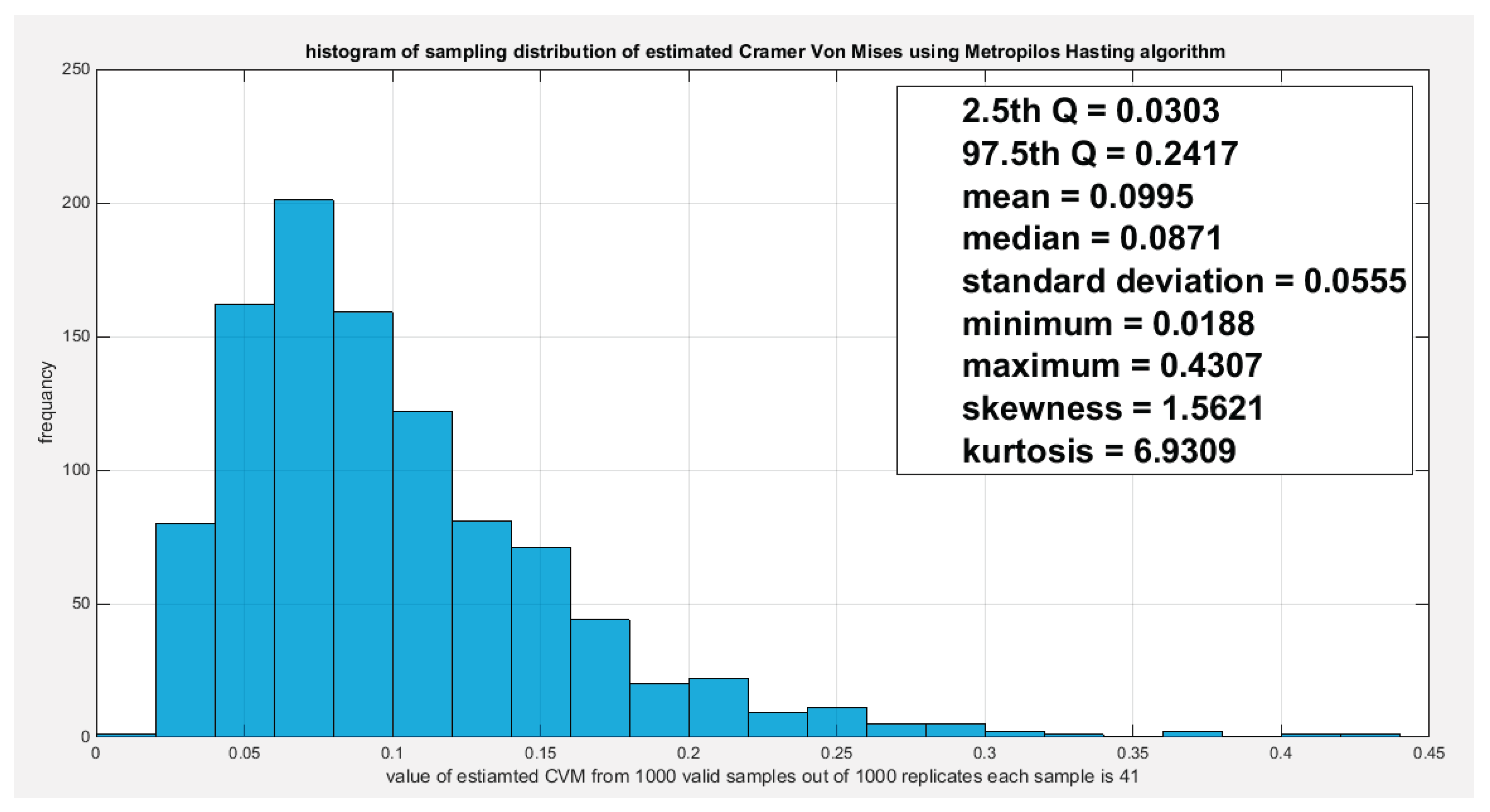
Figure 7.
shows the sampling distribution of the dependency parameter. The 0.5714 lies in the acceptance region between the two quantiles, the 2.5th and the 97.5th quantiles. So the null hypothesis fails to reject its assumption. The p-value (probability of the values being less than or equal to this 0.5714) is 0.2950 which indicates that this 0.5714 is not placed in either zones of rejection.
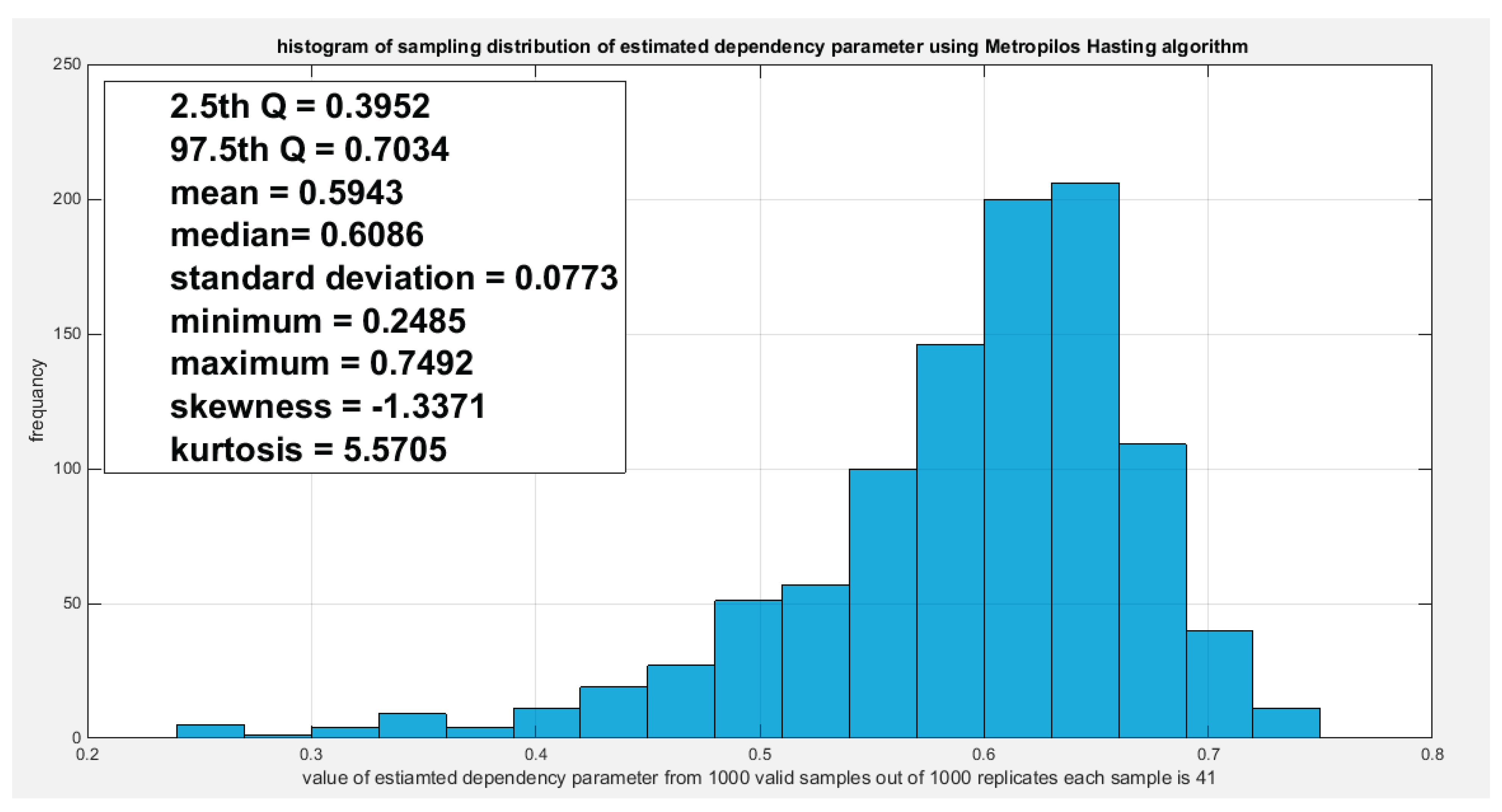
Figure 8.
shows the sampling distribution of the Kendal tau coefficient. Its value 0.5428 is between the two quantiles 2.5th and 97.5th which is the acceptance zones. So the null hypothesis fails to reject its assumption. The p-values (probability of the values less than or equal to 0.5428) is 0.7050 which denotes that this value is far away from both rejection zones.
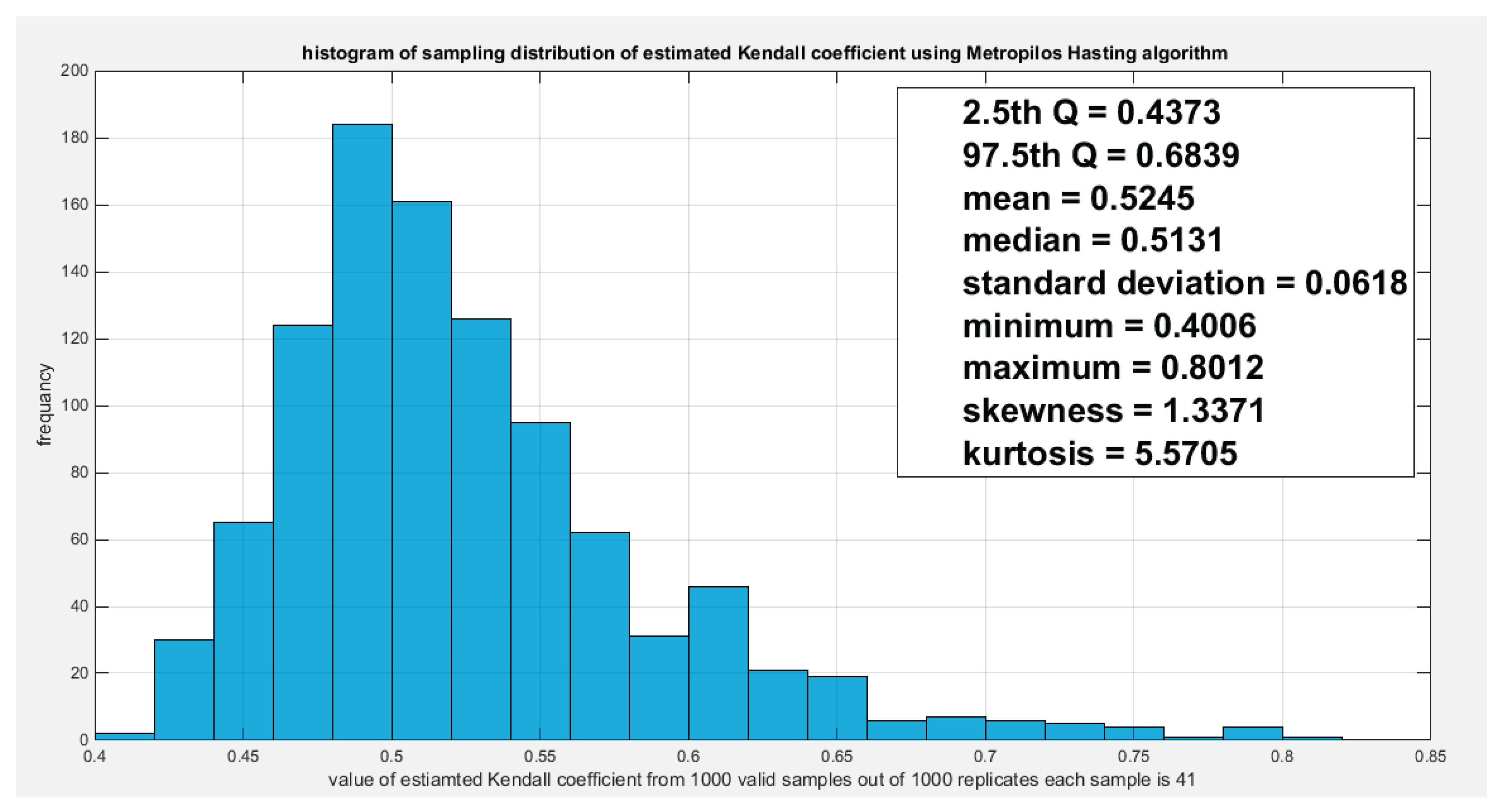
Figure 9.
shows the P-P plot of the empirical vs the theoretical copula. The theoretical copula shows near perfect alignment of its lower and central part with the diagonal line than its upper part.
Figure 9.
shows the P-P plot of the empirical vs the theoretical copula. The theoretical copula shows near perfect alignment of its lower and central part with the diagonal line than its upper part.
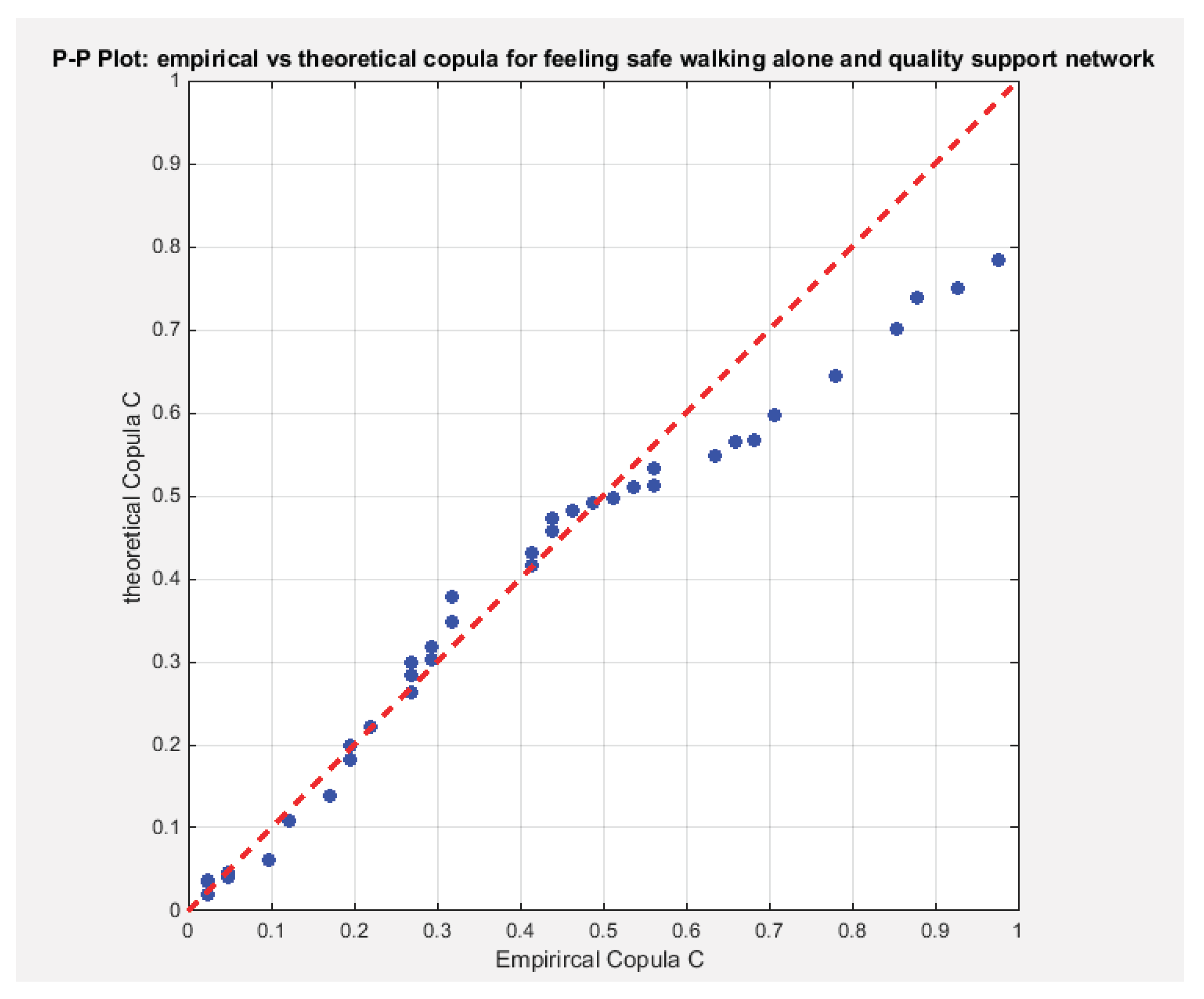
Figure 10.
shows the PDF surface of copula density with parameter 0.5714.
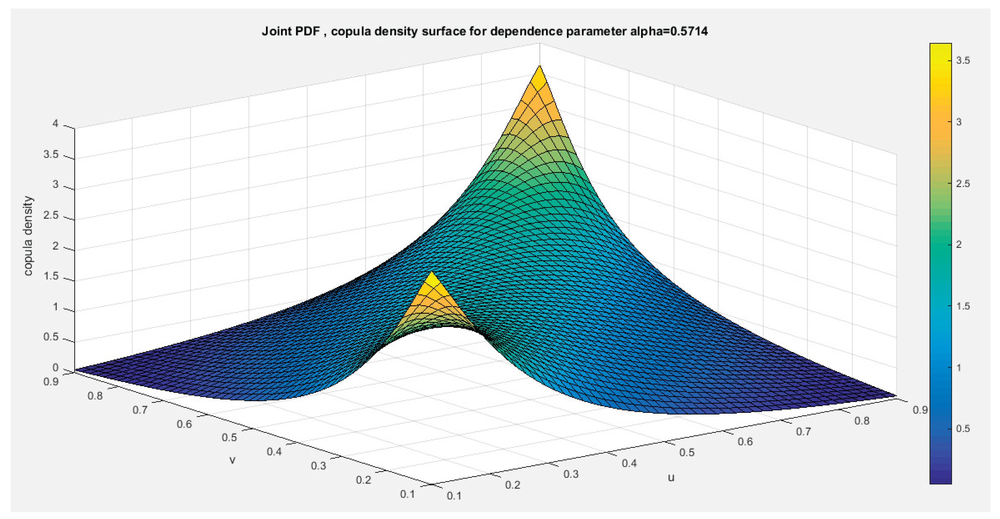
Figure 11.
shows the contour plot of the copula density with parameter 0.5714.
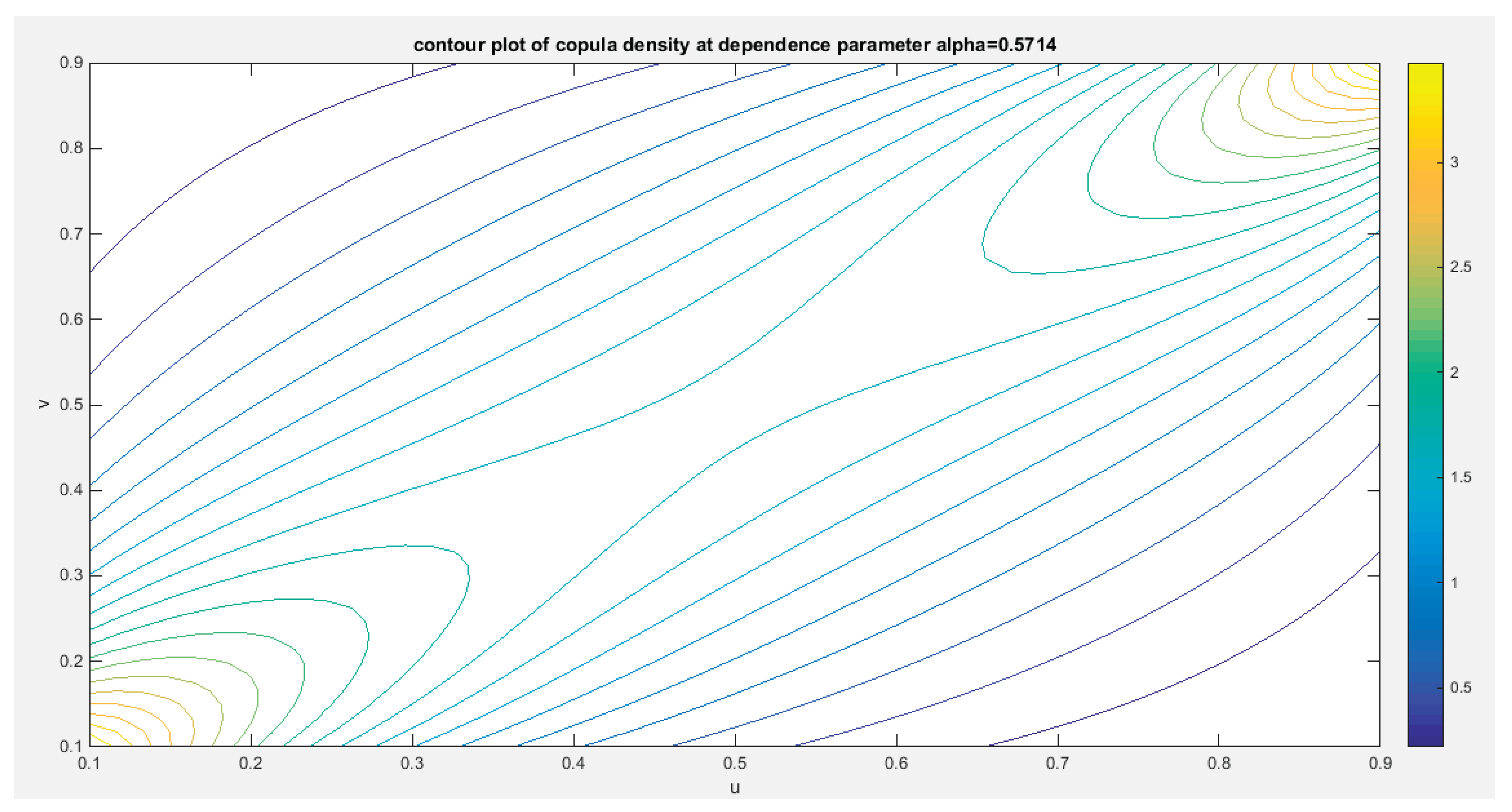
Figure 12.
shows the contour plot of the copula distribution with dependency parameter 0.5714.
9. Conclusions
This copula which is based on frailty model and cox proportional hazard model can only model positive dependency. It can model upper and lower tail dependency. The author discussed one dataset exhibiting left skewness. the copula fit the data well. The complexity of the copula density function dictates uses of IFM method of estimation. This method is favored over the MLE for its simplicity and straightforwardness. The robust variance or sandwich variance captures the covariance between the marginal and the copula parameter estimators which are not captured by separately estimating the variances in each stage. The variance of the estimators of marginal parameters increases while the variance of the estimator of copula parameter decreases. Although the sample size used in the analysis were moderate(n=41), the copula models the upper and lower tail dependency well and this was supported by the sampling distribution of both the empirical upper and lower tail dependency coefficients. These copulas can be used to construct bivariate distributions other than bivariate MBUR as discussed in this paper. While the joint distribution function, for two random variables X and Y, the bivariate density function of these 2 variables is shown in equation (38)
10. Future Work
This copula can be mixed with other copulas to better model data with asymmetric dependency. Also other methods of estimation can be attempted like the semiparametric estimation and MLE. Bayesian inference can also be considered.
Author Contributions
AI (Attia Iman) carried the conceptualization by formulating the goals, aims of the research article, formal analysis by applying the statistical, mathematical and computational techniques to synthesize and analyze the hypothetical data, carried the methodology by creating the model, software programming and implementation, supervision, writing, drafting, editing, preparation, and creation of the presenting work.
Funding
No funding resource. No funding roles in the design of the study and collection, analysis, and interpretation of data and in writing the manuscript are declared
Institutional Review Board Statement
Not applicable.
Informed Consent Statement
Not applicable
Data Availability Statement
AI (Attia Iman) does not analyze or generate any datasets, because her work proceeds within a theoretical and mathematical approach.
Conflicts of Interest
The author declares no competing interests of any type.
References
- Al Turk, L. I.; Abd Elaal, M. K.; Jarwan, R. S. Inference of bivariate generalized exponential distribution based on copula functions. Applied Mathematical Sciences 2017, 11, 1155–1186. [Google Scholar] [CrossRef]
- Alsina, C.; Franks, M. F.; Schweizer, B. Associative Functions.Triangular Norms and Copulas; World Scientific; Singapore, 2006. [Google Scholar]
- Attia, I. A Novel One Parameter Unit Distribution: Median Based Unit Rayleigh: Properties and Estimations. Preprint.org. 2024. [Google Scholar] [CrossRef]
- Attia, M.I. A Novel Unit Distribution Named as Median Based Unit Rayleigh (MBUR):Properties and Estimations. Preprints.Org, Preprint 2024. [Google Scholar] [CrossRef]
- Chen, X. Chapter 76 Large Sample Sieve Estimation of Semi-Nonparametric Models. In Handbook of Econometrics; Elsevier, 2007; pp. 5549–5632. Available online: https://linkinghub.elsevier.com/retrieve/pii/S157344120706076X.
- Cherubini, U.; Luciano, E.; Vecchiato, W. Copula Methods In Finance; John Wiley and Sons, 2004. [Google Scholar]
- Cuadras, C. M.; Fortiana, J.; Rodriguez-Lallena, J. A. Distributions with Given Marginals and Statistical Modellings; Kluwer, 2002. [Google Scholar]
- Drouet-Mari, D.; Kotz, S. Correlation and Dependence; Imperial College Press, 2001. [Google Scholar]
- Durante, F.; Sempi, C. Principles of Copula Theory; CRC Press, 2015. [Google Scholar]
- Embrechts, P.; Lindskog, F.; Mcneil, A. Modelling Dependence with Copulas and Applications to Risk Management. In Handbook of Heavy Tailed Distributions in Finance; Elsevier, 2003; pp. 329–384. [Google Scholar] [CrossRef]
- Frees, E. W.; Valdez, E. A. Understanding Relationships Using Copulas. North American Actuarial Journal 1998, 2(1), 1–25. [Google Scholar] [CrossRef]
- Genest, C. Preface; Candian Journal of statistics, 2005a; Vol. 33. [Google Scholar]
- Genest, C. Preface; Insurance: Mathematics and Economics, 2005b; Vol. 37. [Google Scholar]
- Genest, C.; Mackay, J. The Joy of Copulas: Bivariate Distributions with Uniform Marginals. The American Statistician 1986, 40(4), 280–283. [Google Scholar] [CrossRef]
- Genest, C.; Rémillard, B.; Beaudoin, D. Goodness-of-fit tests for copulas: A review and a power study. Insurance: Mathematics and Economics 2009, 44(2), 199–213. [Google Scholar] [CrossRef]
- Godambe, V. P. (Ed.) Estimating Functions; Oxford University PressOxford, 1991. [Google Scholar] [CrossRef]
- Jaworski, P.; Durante, F.; Hardle, W. Copula in Mathematical and Quantitative Finance; Springer Verlag, 2013. [Google Scholar]
- Jaworski, P.; Durante, F.; Hardle, W.; Rychlik, T. Copula Theory and Its Applications: Proceedings of the Workshop held in Warsaw. Lecture Notes in Statistics; Springer Verlag, 2010; Vol. 198. [Google Scholar]
- Joe, H. Families of min-stable multivariate exponential and multivariate extreme value distributions. Statistics & Probability Letters 1990, 9(1), 75–81. [Google Scholar] [CrossRef]
- Joe, H. Parametric Families of Multivariate Distributions with Given Margins. Journal of Multivariate Analysis 1993, 46(2), 262–282. [Google Scholar] [CrossRef]
- Joe, H. Multivariate Models and Dependence Concepts; Chapman and Hall, 1997. [Google Scholar]
- Joe, H. Asymptotic efficiency of the two-stage estimation method for copula-based models. Journal of Multivariate Analysis 2005, 94(2), 401–419. [Google Scholar] [CrossRef]
- Joe, H. Dependence Modeling with Copulas; CRC Press, 2014. [Google Scholar]
- Joe, H.; Hu, T. Multivariate Distributions from Mixtures of Max-Infinitely Divisible Distributions. Journal of Multivariate Analysis 1996, 57(2), 240–265. [Google Scholar] [CrossRef]
- Kim, G.; Silvapulle, M. J.; Silvapulle, P. Comparison of semiparametric and parametric methods for estimating copulas. Computational Statistics & Data Analysis 2007, 51(6), 2836–2850. [Google Scholar] [CrossRef]
- Kolev, N.; Anjos, U. D.; Mendes, B. V. D. M. Copulas: A Review and Recent Developments. Stochastic Models 2006, 22(4), 617–660. [Google Scholar] [CrossRef]
- Kolev, N.; Paiva, D. Copula-based regression models: A survey. Journal of Statistical Planning and Inference 2009, 139(11), 3847–3856. [Google Scholar] [CrossRef]
- Mai, J. F.; Scherer, M. Finanial Engineering with Copula Explained; Palgrave Macmillan, 2014. [Google Scholar]
- Malevergne, Y.; Sornette, D. Extreme Financial Risks: From Dependence to Risk Management; Springer Verlag, 2006. [Google Scholar]
- Manner, H.; Reznikova, O. A Survey on Time-Varying Copulas: Specification, Simulations, and Application. Econometric Reviews 2012, 31(6), 654–687. [Google Scholar] [CrossRef]
- McNeil, A. J.; Frey, R.; Embrechts, P. Quantitative Risk Management: Concepts, Techniques and Tools; Princeton University Press, 2005. [Google Scholar]
- Nadarajah, S.; Afuecheta, E.; Chan, S. A Compendium of Copulas. Statistica 2018, Vol 77, 279–328 Pages. [Google Scholar] [CrossRef]
- Nelsen, R. B. Cuadras, C. M., Fortiana, J., Rodriguez-Lallena, J. A., Eds.; Concordance and Copulas: A Survey. In Distributions With Given Marginals and Statistical Modelling; Springer Netherlands, 2002; pp. 169–177. [Google Scholar] [CrossRef]
- Nelson, R. B. An Introduction to Copulas; Springer Verlag, 2006. [Google Scholar]
- Ozun, A.; Cifter, A. Estimating Portfolio Risk with Conditional Joe-Clayton Copula: An Empirical Analysis with Asian Equity Markets. The IUP Journal of Financial Economics 2007, V, 28–41. [Google Scholar]
- Patton, A. J. A review of copula models for economic time series. Journal of Multivariate Analysis 2012, 110, 4–18. [Google Scholar] [CrossRef]
- Salvadori, G.; Michele, C. D.; Kottegoda, N. T.; Rosso, R. Extremes in nature. An approach Using Copulas; Springer Verlag, 2007. [Google Scholar]
- Schweizer, B. Dall’Aglio, G., Kotz, S., Salinetti, G., Eds.; Thirty Years of Copulas. In Advances in Probability Distributions with Given Marginals; Springer Netherlands, 1991; pp. 13–50. [Google Scholar] [CrossRef]
- Schweizer, B.; Sklar, A. Probabilistic Metric Space; Dover, Mineola, 2005. [Google Scholar]
- Sklar, A. Random Variables, Joint distribution functions, and copulas. Kybernetika 1973, 9(6), 449–460. [Google Scholar]
- Tsukahara, H. Semiparametric estimation in copula models. Canadian Journal of Statistics 2005, 33(3), 357–375. [Google Scholar] [CrossRef]
- Weiß, G. Copula parameter estimation by maximum-likelihood and minimum-distance estimators: A simulation study. Computational Statistics 2011, 26(1), 31–54. [Google Scholar] [CrossRef]
- Xu, J. J. Statistical modelling and inference for multivariate and longitudinal discrete response data. https://doi.org/10.14288/1.0087914. Ph.d thesis, University of British Columbia, 2009. [Google Scholar]
Disclaimer/Publisher’s Note: The statements, opinions and data contained in all publications are solely those of the individual author(s) and contributor(s) and not of MDPI and/or the editor(s). MDPI and/or the editor(s) disclaim responsibility for any injury to people or property resulting from any ideas, methods, instructions or products referred to in the content. |
© 2025 by the authors. Licensee MDPI, Basel, Switzerland. This article is an open access article distributed under the terms and conditions of the Creative Commons Attribution (CC BY) license (http://creativecommons.org/licenses/by/4.0/).
Copyright: This open access article is published under a Creative Commons CC BY 4.0 license, which permit the free download, distribution, and reuse, provided that the author and preprint are cited in any reuse.


