Submitted:
18 April 2025
Posted:
21 April 2025
You are already at the latest version
Abstract
In this article, a three-dimensional Eyring-Powell nanofluid stream in the presence of gyrotactic microorganisms over the stretched sheet is contracted under the impact of the Hall and Ion slip parameters. The main objective of this research is to examine the three-dimensional flow properties of Eyring-Powell nanofluid with aspects related to mass and heat transfer. The structure of independent partial differential equations is converted into sets of non-linear ordinary differential equations by applying the suitable conversion mechanism. The homotopy analytic strategy is employed to conduct the analytical evaluation of the current work. The skin friction coefficients and the Nusselt number are extracted against distinct flow variables. The relevant parameters are displayed visually and shown to demonstrate the impacts on the zones of velocity, temperature, concentration of nanoparticles, and concentration of gyrotactic bacteria. Furthermore, graphs and tables displaying the results have been created to demonstrate the impact of physical behaviors. The findings of this study are crucial for both academic advancements in the mathematical modelling of Eyring-Powell liquid motion with heat exchange in engineering structures and biomedicine, as well as for practical applications in chilling.
Keywords:
Eyring-Powell nanofluid
; Hall Current
; Ion Slip
; Gyrotactic Microorganisms
; Bioconvection
; Homotopy Analysis Method.
1. Introduction
According to viscosity’s law, two categories of liquids can be encountered in nature. Newtonian fluids and non-Newtonian fluids.
Because there is zero yield tension in a Newtonian fluid, the stress generated by shear is a function that is linear with the shear rate. Due to the complexity of their design and maintenance under the power type model, non-Newtonian fluids might result in an irregular connection among shear stress and shear rate, as shown in Figure 1.
Water, ethanol, and oxygen are a few typical examples of Newtonian materials. Several other liquids are non-Newtonian, meaning that their viscosity changes as their strain rises. The focus of the investigation is the fluid referred to as Eyring-Powell fluid. According to recent scientific research, unlike bioconvection motile creatures, the thermophysical properties in a Powell-Eyring nanofluid across a sheet of stretched material are seldom given. Powell and Eyring developed the Eyring–Powell nanofluid model in 1944 [1]. The purpose of this model is to replicate the substance flow that occurs throughout production. The Eyring-Powell model is a highly intricate, non-Newtonian structure designed for research purposes. However, there are several benefits that this model offers over other non-Newtonian products, such as its physical durability, clarity, and simple calculation. The features of the Eyring-Powell fluid distinguish it from several non-Newtonian simulations and give it importance. Hassan et al. [2] examined the creation of entropy and circulation properties of the Powell Eyring liquid under the influence of time and viscous variables. Sajjad et al. [3] created computational models of magnetism polarity across a nonlinear reactive Eyring-Powell nanofluid that took into account ohmic and fluid dissipation consequences. Abozaid et al. [4] discovered the MHD Powell-Eyring dirty nanofluid stream caused by extending the interface with a heat flow barrier constraint. The intermittent analysis of an Eyring-Powell fluid was investigated by Akbar et al. [5]. Malik et al.et al. [6] evaluated the impact of altering viscosity using Eyring–Powell fluid.
The study of partially ionised matter has gained significant attention in the field of solar physics recently due to its composition in the various layers of the solar wind and solar formations like protrusions and spikes. Solar protrusions are fascinating formations found in the solar corona that are the subject of intense research due to their unique characteristics and behaviors, which are yet unclear. The partially ionised streams reveal radically unique features compared to the regular liquids under magnetic field influence. Ion impacts produce forces such as the ion slip force and the Hall force caused by electron collisions, which partially ionised fluids feel when a magnetic field is introduced. The opposite orientations of the Hall and attraction forces are confirmed in a laboratory study.
Figure 3.
shows the helium ion that is partially ionised.
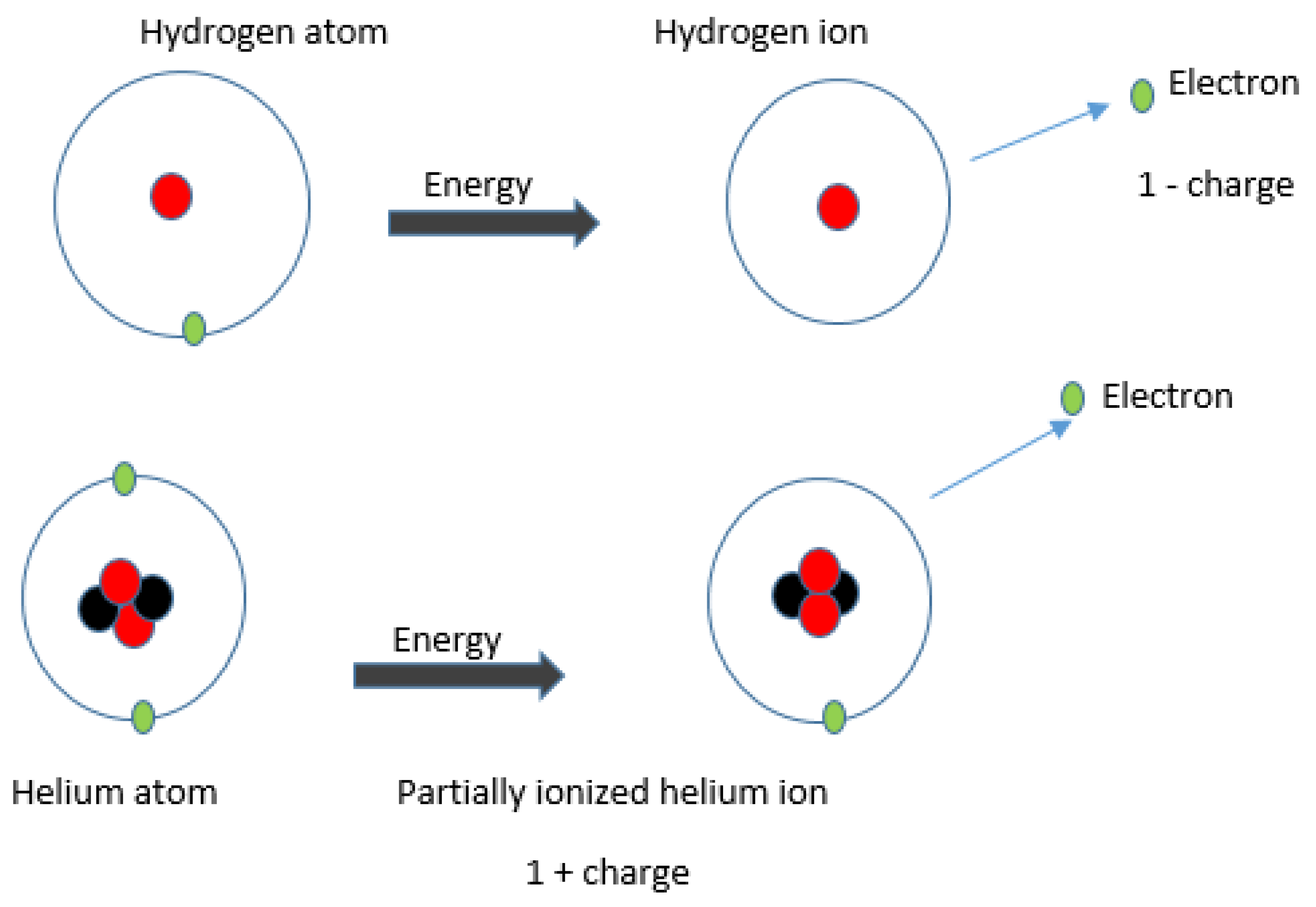
The application of the magnetic field to the partially ionized fluid results in the sensation of several forces. These forces include magnetic force because of the magnetic field. The impact of electrons produces Hall force, whereas the impact of ions produces force due to ion slip winds. These ions slip, and the Lorentz force created by a magnetic field being generated is opposed by Hall effects. Ramzan et al [7] reported the role of biological convection in a 3D tangential hyperbolic partly ionised magnetised nanofluid circulation with Cattaneo-Christov heat exchange and stimulation energy. The 3D nano-plasma circulation concept constructed around Hall and Ion slip winds in the context of thermal radiation was proposed by Qureshi et al [8]. To create their mathematical models, Hayat et al [9] took into account how Ohmic dispersion and Hall currents affected the heat transfer in the peristaltic process produced by mixed convection stream. The influence of Brownian motion and thermophoresis on MHD mixed convection thin-layer second-grade nanofluid circulation with the Hall impact and heat exchange beyond an elastic sheet was investigated by Khan et al [10]. The consequences of Hall and ion slip in the combined convection form of Jeffrey nanofluid were examined by Hayat et al [11]. The three-dimensional variation in temperature in polymer blends with tiny particles in the presence of Hall and Ion slip impacts was studied by Nawaz et al [12]. Using the symmetrical continuous technique, Elshehawey et al [13] examined the effects of Hall and Ion-slip variables on the MHD stream with variable warmth potential.
Microorganisms, which are single-celled organisms, are present in all living things, including humans, animals, and other species. Swimming microorganisms, as shown in Figure 4. Microorganisms are cause the accumulation of bacteria and other gyrotactic microorganisms, which are much thicker than water. Gyrotactic bacteria’s physical and intriguing relevance is efficiently utilized by renewable energy, alcohol, and other atmospheric and ecological systems. Gyrotactic bacteria have applications in several scientific and biotechnological fields, which has piqued the interest of experts and researchers in their occurrence in nanofluids.
There are three different kinds of moving microorganisms: gyrotactic, chemo-tactic, and negative gravity germs. Researchers and scholars have recently focused a great deal of interest on gyrotactic microbial movement in small-molecule fluids. Since they may use the bioconvection technique, gyrotactic bacteria are used at the nanoscale for better fluid mixing. An inquiry into nanotechnology by Dahich et al. [14] demonstrates sisko circulating nanofluid over a constant elastic sheet with moving gyrotactic germs. The study conducted by Mustapha et al. [15] investigated the peristaltic exchange of nanofluid with flexible gyrotactic bacteria under asymmetric thermal radiation. In a heated system, Iqbal et al. [16] studied partially ionised bioconvection Eyring–Powell nanofluid motion with gyrotactic microbes. Khan et al. [17] examined the effects of gyrotactic microbes and nonlinear thermal radiation on the Magneto-Burgers tiny fluids. In an unconventional blood-based tiny fluid, Bhatti et al. [18] experimented using an annular coordinate frame to investigate mobile gyrotactic organisms. They demonstrated that fluid movement behaviour in non-tapered, merging, and divergence capillaries is constant across the entirety of the flow stream. Using inherent shooting skills, Khan et al. [19] revealed the Walter-B fluid impacted by gyrotactic bacteria and the heat transmission phenomenon by looking at the visual and statistical illustration of the issue. Another work by Nima et al. [20] examined gyrotactic microbes in an unconventional fluid across a vertical surface attached to a porous substance. They found that the surface temperature and rate of the unconventional fluid show an inverse pattern for the combined convection variable. Using a shooting approach, Naz et al. [21] presented the behaviour of activation energy in the computational model of the non-Newtonian nanofluid and examined how improving the volumetric resistance of the microscopic particles contributes to an increase in the energy of activation. The References [22,23,24] contain a few more studies on gyrotactic bacteria.
As seen in Figure , the term "nanofluid" describes the element base liquid that has been infused with nanoparticles. The term "nanofluid" refers to a unique class of heat transfer fluids that are obtained through the stable suspension and consistent dispersion of tiny particles in base fluids such as glycol, liquid, gasoline, oil, and bio-fluids. The largest and most promising warmth properties of nanofluid are achieved by using fragments at low concentrations that are adequate.
In numerous real-world scenarios, the nanofluid is crucial. There are several applications of nanofluids in solar energy technology, food, leather, automobiles, and nuclear power industries, as well as heat transfer devices and the cooling of electrical and vehicle systems, as expressed in Figure 5.
At the initial stage, Choi[25] introduced the term "nanomaterials," keeping focus on the general goal of improving the thermal conductivity of nanofluids. A conceptual heterogeneous stability model for the molecular dispersion of nanofluids was developed by Buongiorno[26]. The unconventional nanofluid with radiative and magnetic influences was examined by Waqas et al.[27]. The majority of scientists employ convection warmth or nil mass flux circumstances for their nanofluids, but to make their simulations more plausible and positive, they solved their problems using both of these scenarios. In the end, they concluded that the consequences of radiation require a thicker boundary region layer. According to Akbari et al.[28] evaluation of the thermal exchange impact in a non-Newtonian nanofluid, the velocity of heat transfer rises as the percentage of solid nanoparticles in the nanofluid increases. Ellahi et al.[29] studied the phenomenon of natural convection, in which tiny carbon nanotubes traverse an upward cone while floating in a solution composed of water. Turkyilmazoglu [30] investigated how mass and heat transmission affected the Buongiorno model of nanofluid. A homogeneous MHD movement with heat and mass exchange via a moving narrow needle in a mixture of nanostructures powered by fluid dissipation and heat radiation was examined by Nazar et al.[31] Using an electro-MHD circulation, Bilal et al.[32] examined the non-Newtonian-Williamson nanofluid flow across an expanding sheet.
Using the streaming patterns in the dense cultures of free-swimming microorganisms, Platt [33] first invented the term "bioconvection". Due to the presence of thermal convection, these bacteria seem to be Bernard cells but were not observed by Platt in 1961. Recent studies using bioconvection in nanofluids have attracted the interest of different researchers. In modern engineering and environmental systems, bioconvection has become a key process. This kind of convection is brought about by an unstable stratification of density produced about by up swimming microorganisms. Consider various photosynthetic microorganisms like cyanobacteria and green algae as an example. In biological systems and biotechnology, bioconvection has various uses. Mabood et al.[34] provided empirical modelling of spontaneous convection of unconventional tiny liquids movement in media with pores containing gyrotactic organisms. Rashad et al. [35] looked at a quietly driven tiny liquids approach, that looks more accurate as dynamically regulated designs, to describe the combined transpiration flow of nanofluid including gyrotactic microorganisms inside a vertically structured cylinder. Shaw et al.[36] investigated the biological convection of gyrotactic microbes close to the boundary layer area in a porous media submerged in an angled semi-infinite porosity wall holding water as a base fluid made of motile microbes. Mekheimer and Ramadan[37] discovered the biological convection features of Prandtl nanofluid over porous materials. B’eg et al.[38] explained the bioconvective movement pertinent to nanoliquid in flowing fluctuation area. Their investigation focused on the bioconvection factor’s greater influence on temperature and the number of mobile microorganisms.
Many investigations on the Eyring-Powell fluid flow have been conducted, according to the literature assessment. The transpiration of gyrotactic microorganisms in a nanofluid flow with Hall and ion slip variables past a dynamic stretching interface is adequately explored in this study. The goal of the present effort is to propose a novel study to examine bio-convection generated by gyrotactic microbes in a nanofluid across a stretched sheet with Hall and Ion slip characteristics. The current experiment is unique and unusual because it uses the HAM tool to structure an analytical solution for the Eyring-Powell nanomaterial flow of mass and heat transfer generated from a stretching sheet with random motion and bioconvection. Using mathematical models of Eyring-Powell nanofluid throughout a stretched sheet, this study explores the dynamics of 3D transpiration fluid circulation for mass and warmth transmission, as well as the movement of gyrotactic microorganisms under the influence of the magnetized impact, Hall, and ion slip consequences. The idea of floating motile gyrotactic microbes has garnered significant attention in the past few years because of its potential uses in the fields of biotechnology and other industrial sectors.
1.1. Novelty
The novelty of the present work is that the HAM tool is applied to organise an analytical solution for Eyring-Powell nanomaterial flow of mass and heat transfer produced from a stretching sheet with bioconvection, Hall, ion slip, random motion, heat source, and thermomigration impacts. The novel outcomes provide an improved comprehension of Eyring-Powell fluid flow and heat transport in the presence of bacteria, which will be useful in a variety of engineering and manufacturing applications, including industries, biomedicine, and biofertilizers. Investigated in this study are the responses to the following queries:
- What is the behavior of swimming microorganisms in Eyring-Powell nanofluid?
- How can a magnetic field, Hall, and ion slip traits affect the dynamics of liquid velocity?
- In what way are the gyrotactic bacteria and nanoparticles distributed in three-dimensional Eyring-Powell nanofluid flow?
1.2. Governing Equations
The continuity, velocities, temperature, concentration of nanoparticles, and concentration of gyrotactic microorganisms have the following equations in light of the aforementioned assumptions [39,40,41].
The aforementioned equations control the motion of a Eyring–Powell nanofluid and are listed above. They have to satisfy a set of boundary conditions which are given below,
In the preceding equations, and , respectively, represent the velocity components across the and axis. The T∞ represents the fluid ambient temperature, T denotes the fluid temperature, DB shows the fluid Brownian diffusion coefficient, B0 denotes the strong magnetic field, represents the ion slip parameter, N shows the concentration of microorganisms, N∞ is the ambient concentration of microbes, Tw is the temperature on the wall, is the dynamic viscosity of the fluid, delegates the Hall parameter, shows nanoparticle density, (a, b) are the dimensional constants, Wce is the maximum cell swimming speed, k is the thermal conductivity, is the kinematic viscosity of the nanoparticle, Nw is the reference concentration of microbes, b0 represents the chemotaxis constant, Cw is the wall concentration, cp is the specific heat at constant pressure, is the heat transfer coefficient, C describes the concentration of nanomaterials and C∞ is the ambient concentration. The associated similarity transformation are given below,
1.3. Physical Description of the Problem
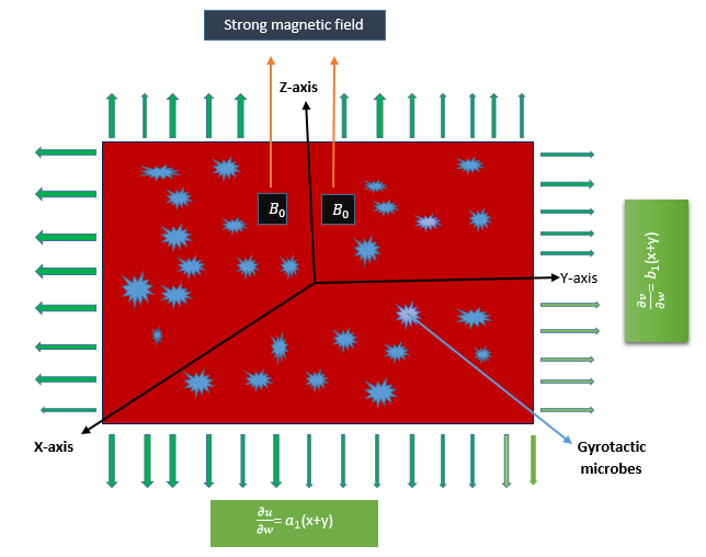
3D Eyring-Powell fluid movement with nanoparticles and gyrotactic microbes in the presence of Hall and ion slip parameters over a stretched sheet, as shown in Figure 6. The concentration of gyrotactic microbes at the wall is Nw and the ambient concentration of the microorganisms profile is N∞. A powerful and consistent magnetic force B0 is delivered from the outside across the z-axis to the stretched sheet, as expressed in Figure 6. The T∞ represents the fluid ambient temperature and Tw is the temperature on the wall of the stretching sheet. The existence of nanoparticles and the speed at which bacteria swim remain unchanged. However, if the size of the fraction of nanoparticles exceeds that, then the mobility of microorganisms is impacted.
where the following variables are represented, in order: gyrotactic microorganisms, temperature, distributions of nanoscale quantity, and speeds , and . The border conditions (7) and controlling partial differential equations (1–6) are converted, applying the similarity transformations, into an arrangement of standard differential equations as follows (8). Equations (1–-6) in its dimensionless structure can be written as,
Boundary conditions are proposed by Iqbal et al.[43].
Here, discuss the various flow parameters in a dimensionless format. Where the dimensionless material parameters are , M is the magnetic field parameter, is the Prandtl number, Nt is the thermophoresis parameter, Nb is the Brownian motion parameter, is the Hall parameter, is the ion slip parameter, is the Concentration difference parameter, Lb is the bioconvection Lewis number, is the thermal relaxation time, Pe is the bioconvection Peclet number, is the Biot number, is the stretching ratio parameter. The values of the parameters are defined as
Where is the local Reynolds number
The physical measurements described previously are shown in the dimensionless format below:
2. Solution of the problem by HAM
The homotopic analysis technique is utilized for the analytic modeling of higher-order nonlinear ordinary differential equations. The Homotopy Analysis Method, a potent analytical strategy, was employed to tackle the problem[44,45,46]. The HAM, a potent analytical strategy, was employed to tackle the problem. When contrasted with other approaches, HAM has numerous benefits, which are given below.
- The convergence solution to the issue at hand is found using this strategy.
- There are no calculations or measurement errors in the HAM.
- There are no baseline units or operators for linearity used in this procedure.
- HAM can be used with both large and small variable schemes.
- This technique can be used for settings with stronger or lower fundamental constants.
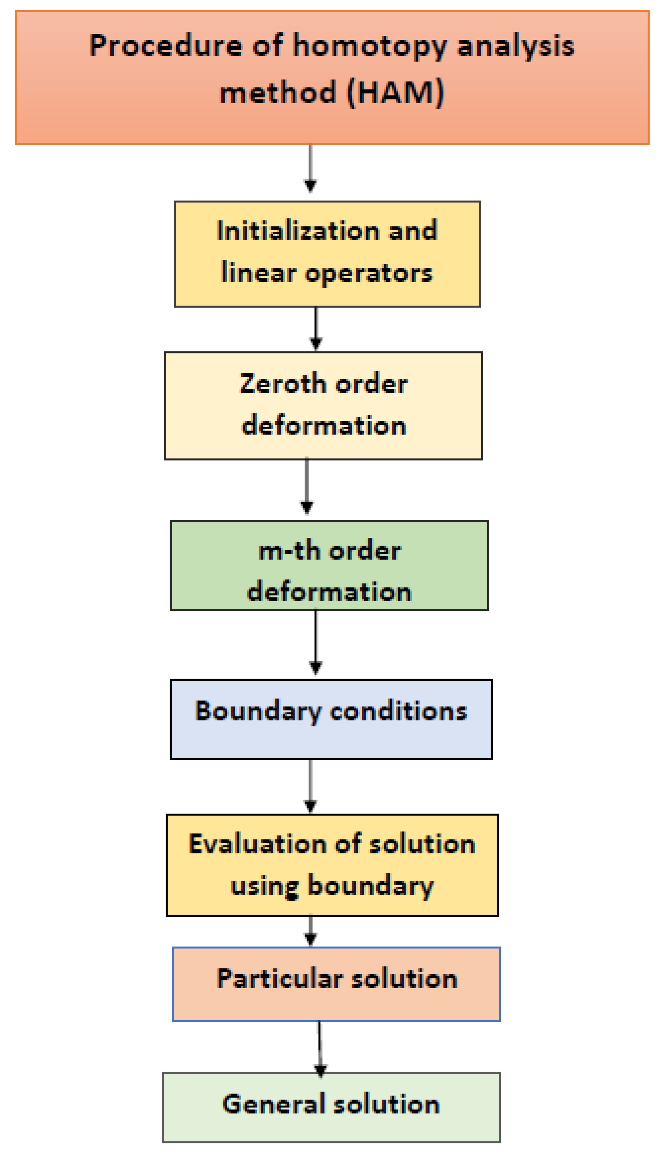
Figure 7.
Demonstrates the homotopy analysis method (HAM) algorithm.
The underlying presumptions and linear operators are conceived to
The values of the random constants are Ji(i = 1–10).
2.1. Deformation Equations of Zeroth Order
where the not a zero supplementary variables are , , , and and q is given as the embedded factor. The definitions of the regressive regulators , , , , and are
Eq. (28–32) has the boundary conditions
For q = 0 and q = 1, Eqs. (23–27) become
Expanding f∼(, q), g∼(, q), (, q), (, q) and (, q) through Taylor series, Eqs. (34–38) generate
From Eqs. (39–43), the convergence of the series is obtained by taking q = 1 for the appropriate values of , , , and , so
2.2. m-th Order Deformation Problems
where
3. Results and Discussion
The black curve in the current system represents the initial impact, the green, blue, and magenta variations start to reflect the eventual behaviour of the profile diminishing and boosting. The behavior of various factors versus motion, heat, and microorganism patterns is described graphically in the present system. Figures illustrate how every emerging parameter impacts temperature, velocity profiles, nanoparticle distributions, and gyrotactic microbe distributions. The primary goal objective of this research project is to examine the 3-D movement behaviour of the Eyring-Powell tiny particles with features related to mass transfer and heat.
3.1. Radial Velocity Profile
The main influences on this research are the electromagnetic field, Hall effect, and ionic slip constants. The consequence of the M on the axial motion of the three-dimensional bioconvect Eyring-Powell nanofluid is discussed in Figure 8. In this case, fluid velocity increases by varying values of M from 0.3 to 0.12. The spike in the nanofluid mobility is evident for escalating values of the , as observed in Figure 9. The fluid velocity has similar behaviour with parameters M and , as depicted in Figure 8 and Figure 9. It is highlighted in Figure 10 by a greater estimation of the Hall parameter, which results in a decreased motion of the fluid. Since the Lorentz force generated via the nanofluid particles decreases the fluid particle’s motion when the Hall influence surpasses, the Eyring-Powell tiny fluid velocity is also reduced. A considerable quantity of frictional force is produced among the particles of fluid as a result of the Hall current surge. Physically, the generation of Lorentz pressures that reduced the nanoparticles’ velocity because of resistance improves the efficiency of thermal transmission. Figure 11 expresses the impact of the thermal relaxation factor on the Eyring-Powell nanofluid velocity . The nanofluid’s mobility rises by values ranging from 0.2 to 0.8, as showed in Figure 11. The consequence of the stretching ratio parameter on the transverse velocity of the bioconvect Eyring-Powell nanofluid is investigated in Figure 12.
3.2. Transverse Velocity Profile
Figure 13 and Figure 14 reflect the effect of the M and the ion slip over the transverse velocity curve. The implications of M and the over a transverse velocity field are indicated in Figure 13 and Figure 14. It is observed that when the Hall current and magnetic parameter M values increase, the velocity field declines. The reason that the motion of fluid slows down is because of the Lorentz forces, which oppose the movement of the liquid particle. Figure 15 illustrates the implications of ion slip number on the Jeffery fluid’s velocity profile. The ion slip effect is physically obtained by multiplying high frequency and ion impact together. As seen in Figure 15, an decrease in the nanofluid velocity is evident for escalating values of the ion slip parameter . The consequence of the stretching ratio parameter on the transverse stream of the bioconvect Eyring-Powell liquid is investigated in Figure 16.
3.3. Temperature Profile
In this portion, the temperature profile is clearly explained against different parameters. The intense heat killed some bacteria. Most living creatures cannot withstand extremely hot or extremely cold temperatures, although some can withstand temperatures as high as freezing.The behavior of the with the Hall effect is depicted in Figure 17. The rate of thermal transmission improves with varying values of the Hall parameter, as determined in Figure 17. The ambient temperature gain led the tiny particles to come into contact more frequently, which is the reason for this. The consequence of on the temperature profile of the 3-D bio-convect Eyring-Powell nanofluid is illustrated in Figure 18. Physically, the combination of ion impact period and cyclotron speed is called the ion slip parameter. The large estimation of ion slip generates the maximum collision time and cyclotron frequency. The heat boundary membrane toughness rises by enhancing the ion slip parameter. Figure 18. is sketched to reveal the influence of the on the heat transfer profile as exhibits in Figure 20. Physically speaking, heat diffusion and have an opposite relationship, while represents the excess of particulate dispersion over heat diffusion. An increase in the value lowers thermal diffusivity, which ultimately causes the temperature of the medium to decline, as determined in Figure 20.
3.4. Nanoparticle Concentration Profile
In this part, discuss the nanopartcles concentration profile versus the various parameters and physical behaviour. Transporting nanoparticles from a hot region to a freezing region due to a temperature variation is the physical aspect of the thermophoresis scenario. A mechanism known as thermophoresis happens when various kinds of moveable nanofluid particles are combined jointly and respond variously to the pulling force of a temperature dispersion. Figure 21 displays the 3D Eyring-Powell liquid’s nanoparticle concentration graph for a spectrum of t values. The illustration below demonstrates that increasing the t causes the concentration of nanoparticles in the Eyring-Powell nanofluid to reduce. b influence is responsible for the reduced thickness of the concentration profile’s transitional area, as Figure 22. makes clear. A reduction in concentration causes a boost in the physical randomized flow, which drives nanoparticles to migrate in random paths and at different rates among nanoparticles. The Brownian motion is the unsteady, erratic movement of nanofluid droplets. Physically, if random flow increases, nanoparticles move at various rates and in a variety of directions. As the mobility of the particles increases, the level of nanomaterials falls. In the present system, t and b have a reversal effect on the nanoparticle concentration profile, as illustrated in Figure 21 and Figure 22. The summary seems fairly accurate. Figure 23 demonstrates variation in the curve of the 3D bio-convect Eyring-Powell nanofluid stream concentration against the Sc. Physically, the Schemit number is the ratio of the Brownian diffusion coefficient to the kinematic viscosity of the nanofluid. Large Schemit number estimations allow Brownian diffusion to increase, which is evident in the elevated nanofluid concentration in Figure 23.
3.5. Gyrotactic Microorganisms Profile
This section illustrates how gyrotactic bacteria behave according to different parameter estimations. In Figure 24 indicates the impacts of the on the gyrotactic microbial pattern. The wall thickness of gyrotactic microorganisms increases with the significant estimates of the Bioconvection Levis number. Due to the bioconvection phenomena, the density of movable microorganisms on plate surfaces rises. In Figure 24, the impact of Pe on the zone of the gyrotactic bacteria is demonstrated. Physically, the ratio of cell swimming motion to rat diffusion is called the peclet number. When peclet number is enhanced, the diffusivity of gyrotactic microorganisms falls because of the correlation between the and the diffusion of gyrotactic bacteria. As an outcome of the peclet number, gyrotactic microbe diffusion declined, as demonstrated in Figure 25. The profile of gyrotactic microorganisms is depicted in Figure 26 due to the variation in the concentration difference parameters . As seen in Figure 25 and Figure 26, the and have identical impacts on the gyrotactic organism profile. Because there is a correlation between peclet number and gyrotactic bacterial diffusion, increasing peclet number causes a decrease in the dispersion of gyrotactic microbes. Gyrotactic bacteria diffusion decreased as a result of the peclet number, as shown in Figure 25.
3.6. Tubular Description
Table 1 displays a comparison of frictional coefficients as published by [32]. Table 1 presents numerical values that replicate the impacts of several parameters on skin friction coefficients and the Nusselt number, including the magnetic field parameter M, the fluid, Hall, and ion slip parameters, and Pr. The knowledge gathered from the current work’s homotopy analysis technique answer is entirely consistent with findings obtained using the FEM, or finite element method, that have already been presented [37]. Table 2 and Table 3 describe the numerical calculation of the skin coefficients of friction , and against growing variations in the magnetic parameter M, the Hall current parameter, and the ion slip number. This investigation examines the relationship between the skin friction coefficient and increasing magnetic parameter M estimate and decreasing skin friction coefficient due to ion-slip number and Hall current parameter.
3.7. Final Remarks
Investigating the bioconvection circulation of a 3D Eyring-Powell nanofluid across a stretch sheet in the presence of gyrotactic microorganisms is the primary goal of this work. The physical limitations of the Nusellt number and skin friction coefficients are investigated and found to be in close agreement with previous research for a 3D Eyring-Powell nanofluid. The findings of this study have important implications for both theoretical developments in the mathematical modelling of Eyring-Powell fluid flow. Benefits of the current work include heating and cooling systems, the plastics industry, and numerous other manufacturing and engineering endeavors. The future work will cover a wide range of industrial domains and solar systems, with a focus on heating and cooling systems. Some of the most important results from the current study are as follows:
- The radial velocity profile is enhanced with parameters M and , but velocity is reduced with parameters d2 and .
- The fluid velocity slows down in the transverse direction with parameters M, , and .
- The temperature profile is raised with parameters , , S3, and Pr.
- The concentration of the nanoparticle grows with parameters and Sc, while it is reduced with parameter .
- The concentration of the gyrotactic microbe profile grows with parameter Lb, while it is reduced with parameters Pe and .
Nomenclature
| M | Magnetic field parameter | Concentration difference parameter | |
| Nt | Thermophoresis parameter | Nb | Brownian motion parameter |
| Wce | Maximum cell swimming speed | Lb | Bioconvection Lewis number |
| Prandtl number | Heat transfer coefficient | ||
| B0 | Strong magnetic field | T∞ | Ambient temperature (k) |
| N | Concentration of microorganisms | (u,v,w) | Components of velocity () |
| DT | Thermophoretic diffusion coefficient | C∞ | Ambient concentration |
| b0 | Chemotaxis constant | Cw | Surface concentration |
| T | Fluid temperature (k) | C | Concentration |
| DB | Brownian diffusion coefficient | Tw | Temperature on wall (k) |
| Dn | Diffusivity of microbes | f | Axial velocity profile |
| g | Transverse velocity profile | N∞ | Ambient concentration of microbes |
| cp | Specific heat at constant pressure | Axis coordinates (m) | |
| k | Thermal conductivity | Nw | Reference concentration of microbes |
| (a, b) | Dimensional constants | Pe | Bioconvection Peclet number |
| , | Drag force | Sc | Schmidt number |
| Greek Letters | |||
| Dynamic viscosity | Kinematic viscosity of nanopartcles | ||
| Density of nanoparticle() | Stefan-Boltzmann constant | ||
| Similarity variable | Hall parameter | ||
| Concentration profile | Temperature profile | ||
| Ion slip parameter | Gyrotactic microorganisms profile | ||
| Surface shear stress | d2 | Thermal relaxation time |
References
- R. E. Powell., H. Eyring, Mechanism for relaxation theory of viscosity, Nature. 154(55): 427–428 (1944).
- M. Hassan., M. Ahsan., Usman., M. Alghamdi., T. Muhammad. Entropy generation and flow characteristics of Powell Eyring fluid under effects of time sale and viscosities parameters. natureportfolio. 8376 (2023).
- R. Sajjad., M. Mushtaq., S. Farid., K. Jabeen., R. M. A. Muntazir. Numerical Simulations of Magnetic Dipole over a Nonlinear Radiative Eyring–Powell Nanofluid considering Viscous and Ohmic Dissipation Effects. Mathematical Problems in Engineering. 16 (2021).
- O. A. Abo-zaid1., R. A. Mohamed1., F. M. Hady., A. Mahdy1., MHD Powell–Eyring dusty nanofluid flow due to stretching surface with heat flux boundary condition. Journal of the Egyptian Mathematical Society. 29: 14 (2021).
- N.S. Akbar, Application of Eyring-Powell fluid model in peristalsis with nanoparticles, J. Comput. Theor. Nanosci. 12(1): 94–100 (2015).
- M.Y. Malik., S. Bilal., M. Bibi., U. Ali., Logarithmic and parabolic curve fittinganalysis of dual stratified stagnation point MHD mixed convection flow of Eyring- Powell fluid induced by an inclined cylindrical stretching surface, Results Phys. 7: 544–552 (2017).
- M. Ramzan., H. Gul., S. Kadry., Y. Chu. Role of bioconvection in a three-dimensional tangent hyperbolic partially ionized magnetised nanofluid flow with Cattaneo-Christov heat flux and activation energy. International Communications in Heat and Mass Transfer. 120: 104994 (2021).
- I. H. Qureshi., M. Nawaz., A. Shahzad. Numerical study of dispersion of nanoparticles in magnetohydrodynamic liquid with Hall and ion slip currents. AIP Adv. 9: 025219 (2019).
- T. Hayat., H. Zahir., A. Alsaedi., B. Ahmad. Hall current and Joule heating effects on peristaltic flow of viscous fluid in a rotating channel with convected boundary conditions. Results Phys. 7: 2831–2836 (2017).
- N. S. Khan., T. Gul., S. Islam., A. Khan., Z. Shah. Brownian motion and thermophoresis effects on MHD mixed convective thin film second-grade nanofluid flow with Hall effect and heat transfer past a stretching sheet J. Nanofluids. 6: 812–29 (2017).
- T. Hayat., M. Awais., H. Zahir., A. Saedi., B. Ahmad. Hall current and joule heating effects on the mixed convection peristaltic flow of viscous fluid in a rotating channel with convective boundary conditions, Results Phys. 7: 2831–2836 (2017).
- M. Nawaz., S. Rana., I. H. Qureshi., T. Hayat. Three-dimensional heat transfer in the mixture of nanoparticles and micropolar MHD plasma with Hall and ion effects, Results Phys. 8: 1063–1073 (2018).
- E. F. Elshehawey., N. T. Eldabe., E. M. E. Elbarbary., N. Z. Elgazery., Chebyshev finite-difference method for the effects of hall and ion-slip currents on magnetohydrodynamic flow with variable thermal conductivity, Can. J. Phys. 82: 701–715 (2004).
- Y. Dadhich., R. Jain., K. Loganathan. M. Abbas., K. S. Prabu., M. S. Alqahtani. Sisko nanofluid flow through exponential stretching sheet with swimming of motile gyrotactic microorganisms: An application to nanoengineering. Open Physics. 21: 20230132 (2023).
- D. R. Mostapha., N. T. M. El-dabe. Peristaltic transfer of nanofluid with motile gyrotactic microorganisms with nonlinear thermic radiation. natureportfolio. 13: 7054 (2023).
- M. Iqbal., N. S. Khan., W, Khan., S. B. H. Hassine., S. A. Alhabeeb., H. A. E. Khalifa.Partially ionized bioconvection Eyring–Powell nanofluid flow with gyrotactic microorganisms in thermal system. Thermal Science and Engineering Progress. 47: 102283 (2024).
- M. Khan., M. Irfan., W. A. Khan. Impact of nonlinear thermal radiation and gyrotactic microorganisms on the Magneto-Burgers nanofluid. International Journal of Mechanical Sciences. 130: 375-382 (2017).
- M. M. Bhatti., M. Marin., A. A. Zeeshan., R. Ellahi., S. I. Abdelsalam. Swimming of motile gyrotactic microorganisms and nanoparticles in blood flow through anisotropically tapered arteries. Front. Phys. 8: 95 00095 (2020).
- M. I. Khan., F. Alzahrani., A. Hobiny. Heat transport and nonlinear mixed convective nanomaterial slip flow of Walter-B fluid containing gyrotactic microorganisms. Alex. Eng. J. 59(3): 1761–1769 (2020).
- N. I. Nima. Melting effect on non-Newtonian fluid flow in gyrotactic microorganism saturated non-darcy porous media with variable fluid properties. Appl. Nanosci. 10(10): 3911–3924 (2020).
- S. Naz., M. M. Gulzar., M. Waqas., T. Hayat., A. Alsaedi. Numerical modeling and analysis of non-Newtonian nanofluid featuring activation energy. Appl. Nanosci. 10(8): 3183–3192 (2020).
- N.S. Khan, Q. Shah, A. Bhaumik, P. Kumam, P. Thounthong, I. Amiri, Entropy generation in bioconvection nanofluid flow between two stretchable rotating disks, Sci. Rep. 10 (2020) 4448.
- N.S. Khan, Mixed convection in mhd second grade nanofluid flow through a porous medium containing nanoparticles and gyrotactic microorganisms with chemical reactions, Filomat. 33 (14): 4627–4653 (2019).
- S. Zuhra., N.S. Khan., M. Alam., S. Islam., A. Khan. Buoyancy effects on nanoliquids film flow through a porous medium with gyrotactic microorganisms and cubic auto catalysis chemical reaction, Adv. Mech. Eng. 12 (1): 1–17 (2019).
- S. U. S. Choi., J. Eastman., Enhancing thermal conductivity of fluids with nanoparticles. ASME. 231: 718–720 (2001).
- J. Buongiorno. Convective transport in nanofluids. J. Heat Transf. 128: 240–250 (2006).
- M. Waqas., S. Jabeen., T. Hayat., S. A. Shehzad., A. Alsaedi. Numerical simulation for nonlinear radiated Eyring-Powell nanofluid considering the magnetic dipole and activation energy. Int. Commun. Heat Mass Transf. 112: 104401 (2020).
- O. A. Akbari., D. Toghraie., A. Karimipour., A. Marzban., G. R. Ahmadi. The effect of velocity and dimension of solid nanoparticles on heat transfer in non-Newtonian nanofluid. Physica E Low Dimens. Syst. Nanostruct. 86: 68–75 (2017).
- R. Ellahi., A. Zeeshan., A. Waheed., N. Shehzad.S. M. Sait. Natural convection nanofluid flow with heat transfer analysis of carbon nanotubes–water nanofuid inside a vertical truncated wavy cone. Math. Methods Appl. Sci. 1–19 (2021).
- M. Turkyilmazoglu. On the transparent effects of Buongiorno nanofluid model on heat and mass transfer. Eur. Phys. J. Plus 136(4): 1–15 (2021).
- T. Nazar., M. M. Bhatti., E. E. Michaelides. Hybrid (Au-TiO2) nanofluid flow over a thin needle with magnetic field and thermal radiation: Dual solutions and stability analysis. Microfluid Nanofluidics. 26(2): 12 (2022).
- M. Bilal., M. Ramzan., Y. Mehmood., T. Sajid., S. Shah. M. Y. A. Malik. Novel approach for EMHD Williamson nanofluid over nonlinear sheet with double stratification and Ohmic dissipation. J. Process Mech. Eng. 0(0): 1–16 (2021).
- J. R. Platt., “Bioconvection patterns in cultures of free-swimming microorganisms,”.Science. 133: 1766–1767 (1963).
- F. Mabood., W. A. Khan., A. Izani., M. Ismail. Analytical modeling of free convection of non-Newtonian nanofluids flow in porous media with gyrotactic microorganisms using OHAM. In AIP Conference Proceedings ICOQSIA Langkawi, Malaysia.(2014).
- A. M. Rashad., A. J. Chamkhab., B. Mallikarjunac., M. M. M. Abdoua. “Mixed bioconvection flow of a nanofluid containing gyrotactic microorganisms past a vertical slender cylinder,” Frontiers in Heat and Mass Transfer (FHMT). 10(21): (2018).
- S. Shaw. P. Sibanda. A. Sutradhar. P. V. S. N. Murthy. Magnetohydrodynamics and soret effects on bioconvection in a porous medium saturated with a nanofluid containing gyrotactic microorganisms. ASME J Heat Transfer. 136: 052601 (2014).
- Mekheimer K.S., Ramadan S.F. New insight into gyrotactic microorganisms for bio-thermal convection of Prandtl nanofluid over a stretching/shrinking permeable sheet. SN Appl. Sci. 450: 1–11 (2020).
- , Anwar M.J., Khan W.A. Bioconvective non-Newtonian nanofluid transport in porous media containing micro-organisms in a moving free stream. J. Mech. Med. Biol. 15 (2015).
- M. Nawaz., H.Q. Imran., A. Shahzad. Thermal performance of partially ionized Eyring–Powell liquid: A theoretical approach, Phys. Scripta. 94: 10 (2019).
- M. Ramzan., H. Gul., S. Kadry., Y. M. Chu. Role of bioconvection in a three dimensional tangent hyperbolic partially ionized magnetized nanofluid flow with Cattaneo-Christov heat flux and activation energy, Int. Commun. Heat Mass Trans. 120: 104994 (2021).
- M. Iqbal., N. S. Khan., W. Khan., S. B. H. Hassine., S. A. Alhabeeb., H. A. E. Khalifa. Partially ionized bioconvection Eyring–Powell nanofluid flow with gyrotactic microorganisms in thermal system. Thermal Science and Engineering Progress. 47: 102283 (2024).
- Liao S 2012 Homotopy analysis method in non-linear differential equations Higher Education Press Beijing and Springer-Verlag Berlin Heidelberg. [CrossRef]
- Liao S 2004 On the homotopy analysis method for non-linear problems Appl. Maths. Computat. 147 (Elsevier) 499–513.
- Liao S 1998 Homotopy analysis method: a new analytic method for non-linear problems Appl. Maths. Mech. (English edn, vol. 19, No. [CrossRef]
- M. Iqbal., N. S. Khan., W. Khan., S. B. H. Hassine., S. A. Alhabeeb., H. A. E. Khalifa. Partially ionized bioconvection Eyring–Powell nanofluid flow with gyrotactic microorganisms in thermal system. Thermal Science and Engineering Progress. 47: 102283 (2024).
- M. Ramzan., H. Gul., S. Kadry., Y. M. Chu. Role of bioconvection in a three dimensional tangent hyperbolic partially ionized magnetized nanofluid flow with Cattaneo-Christov heat flux and activation energy. Int. Commun. Heat Mass Trans. 120 104994 (2021).
Figure 1.
depicts the non-Newtonian vs Newtonian fluid.
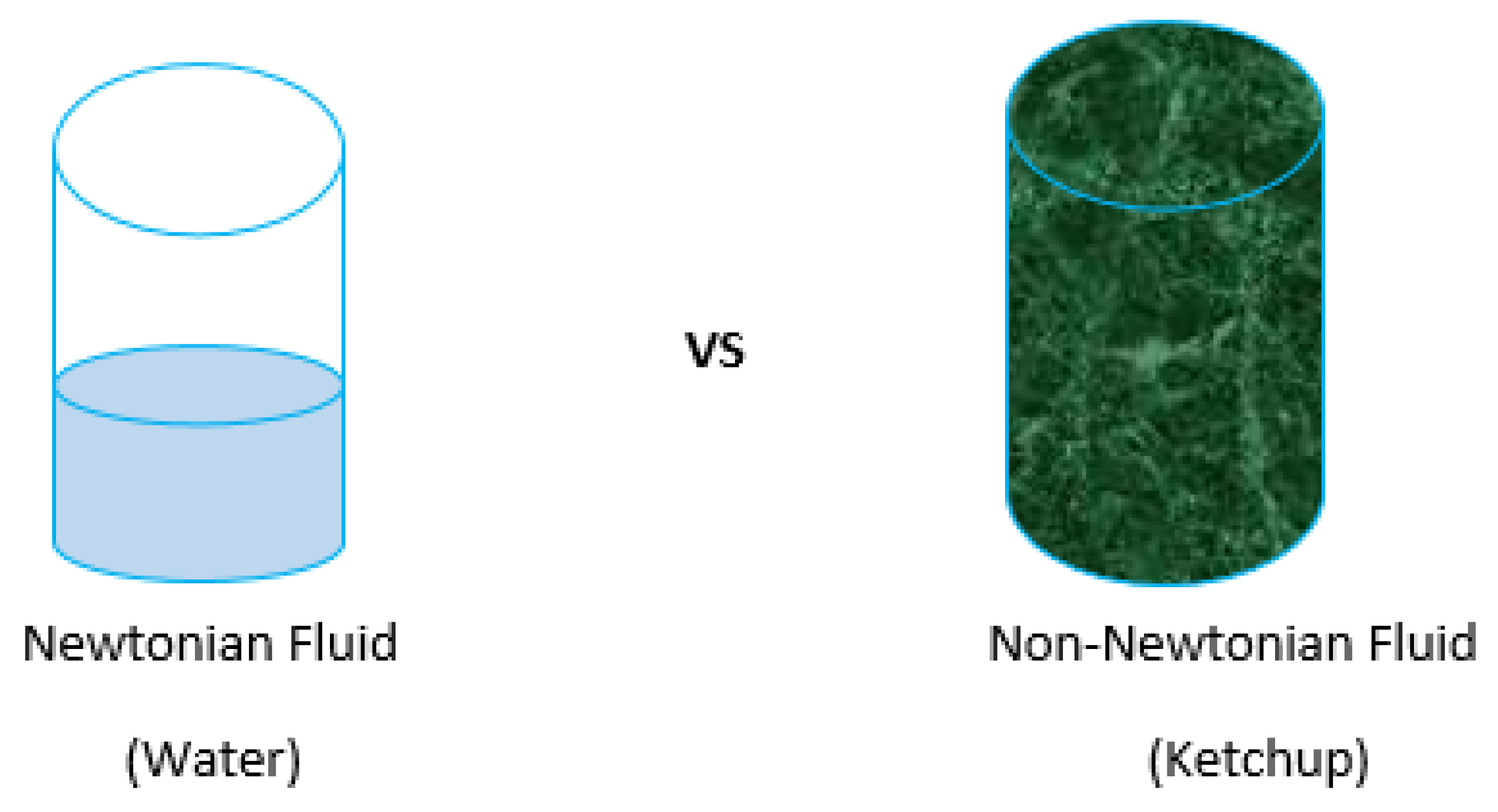
Figure 2.
depicts the non-Newtonian fluid model with relation to strain and shear stress.
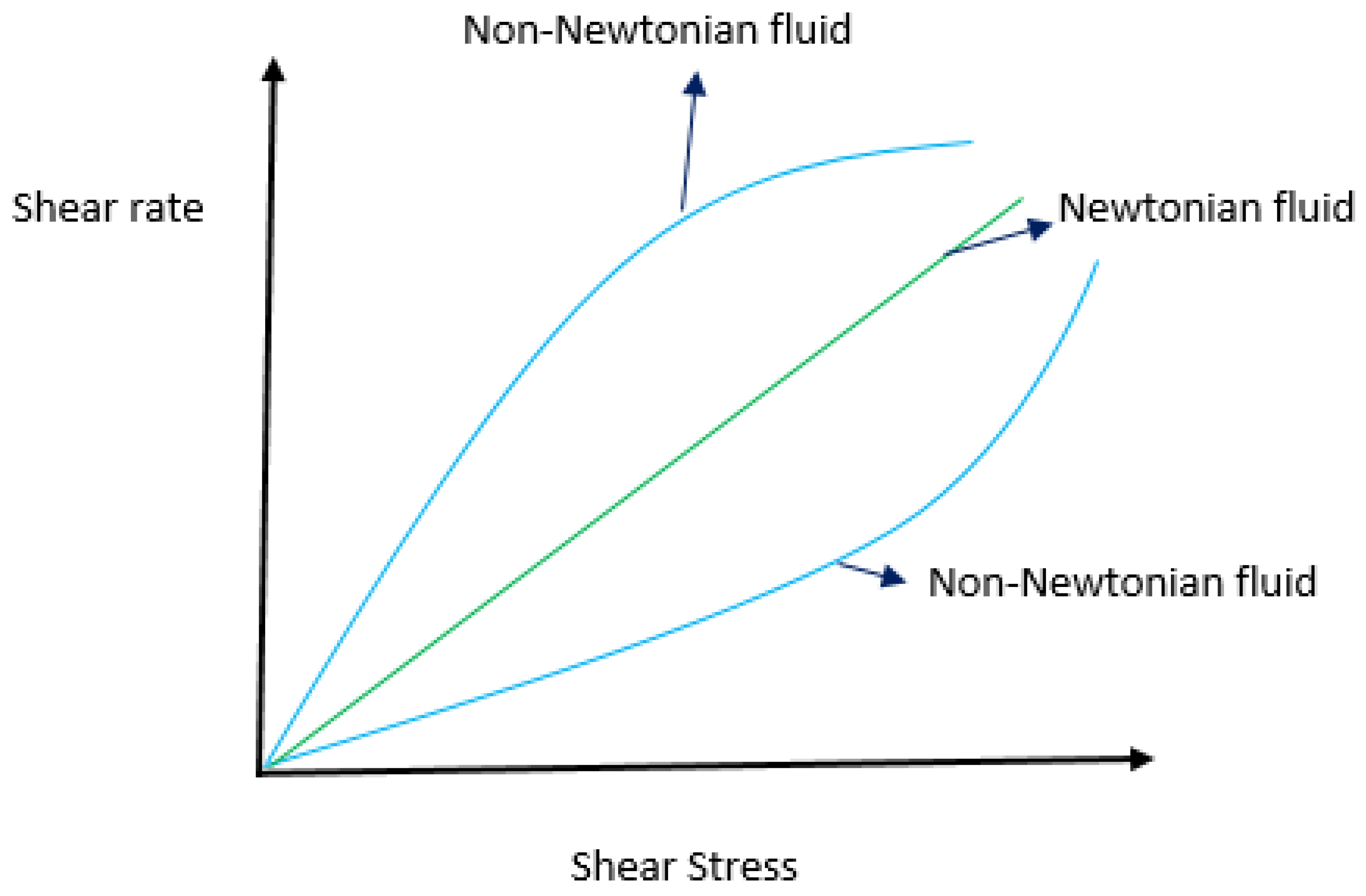
Figure 4.
displays the swimming microorganisms.
Figure 5.
Depicting applications of the nanofluids.
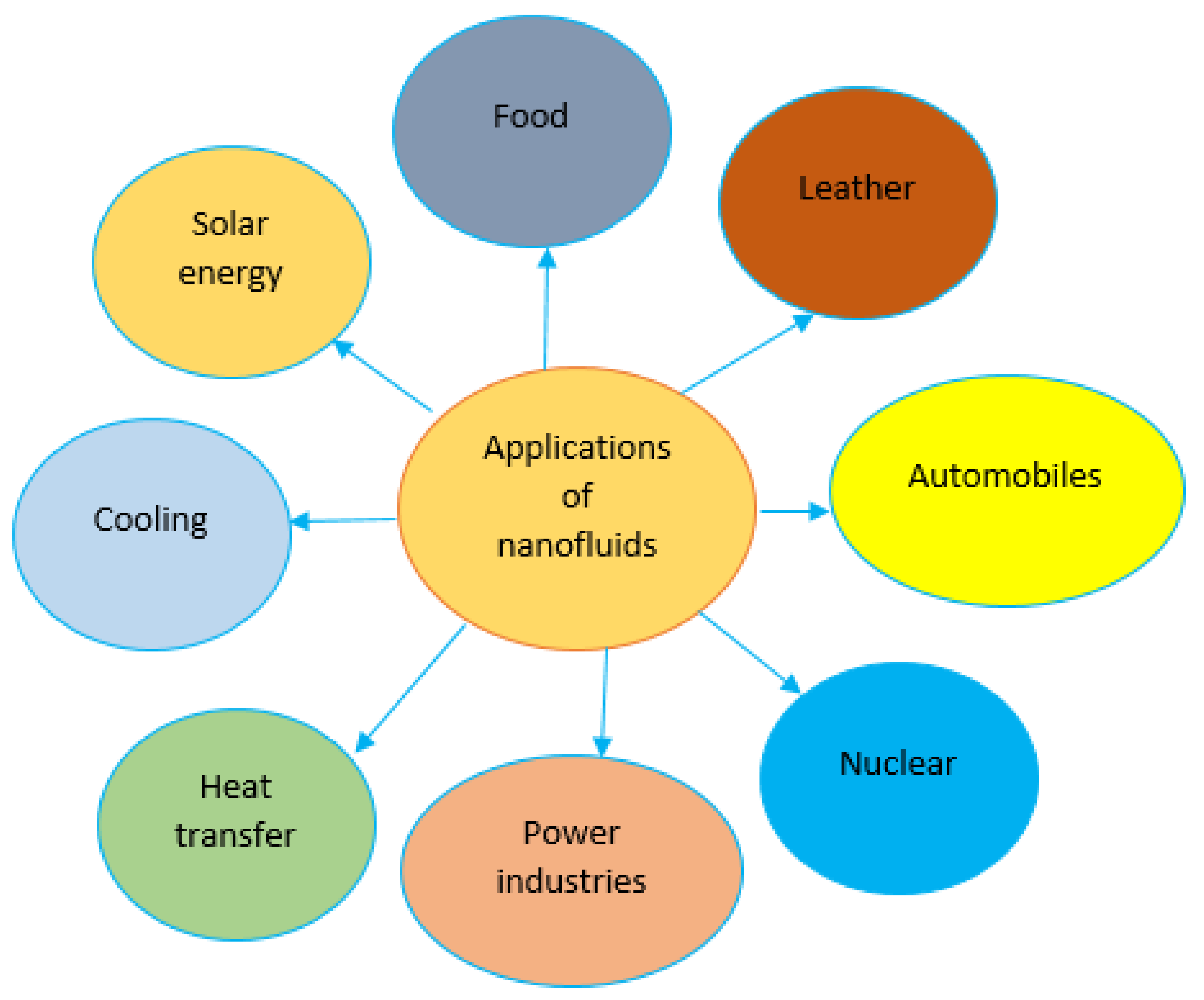
Figure 6.
Flow geometry of the problem.
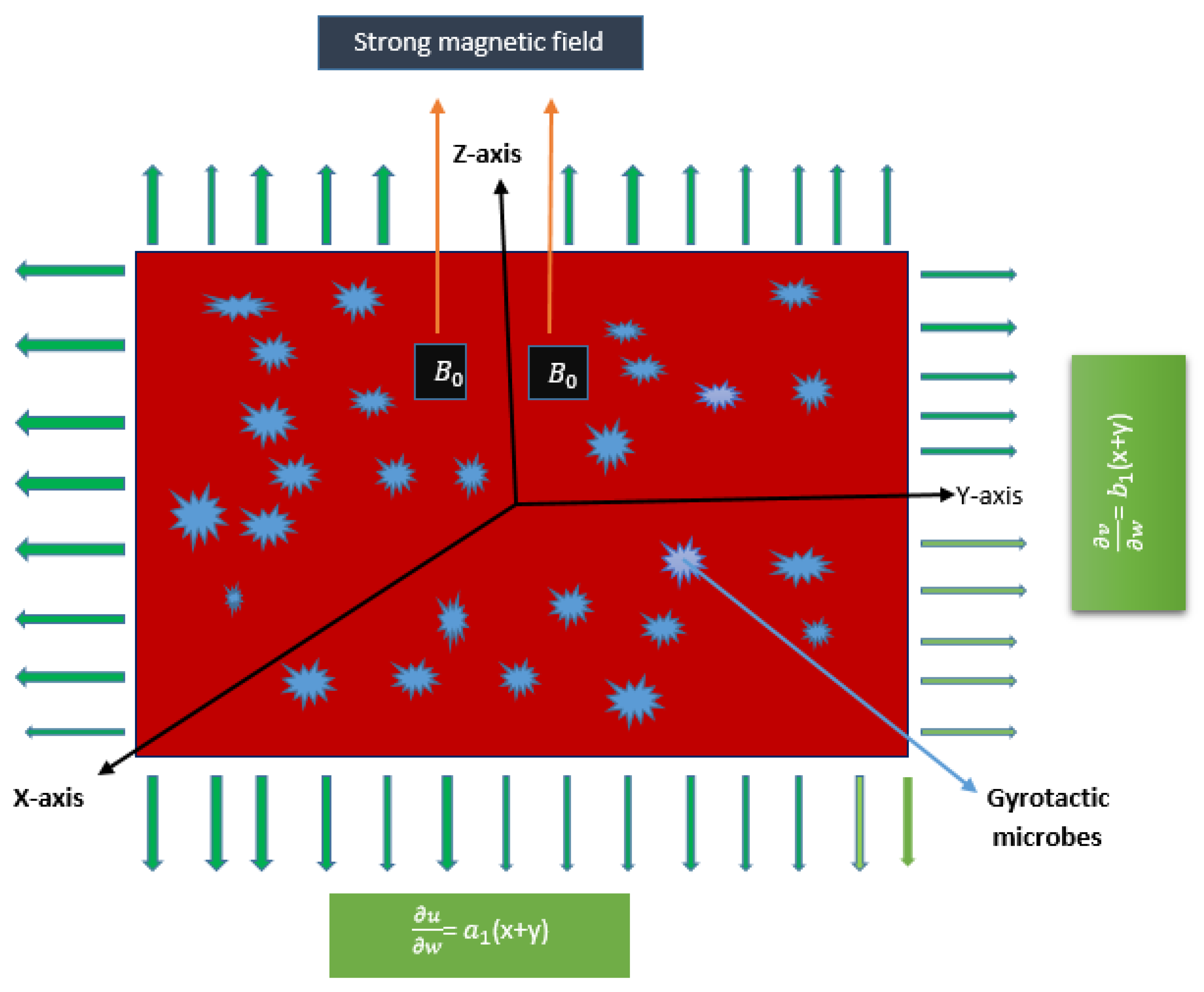
Figure 8.
The against M.
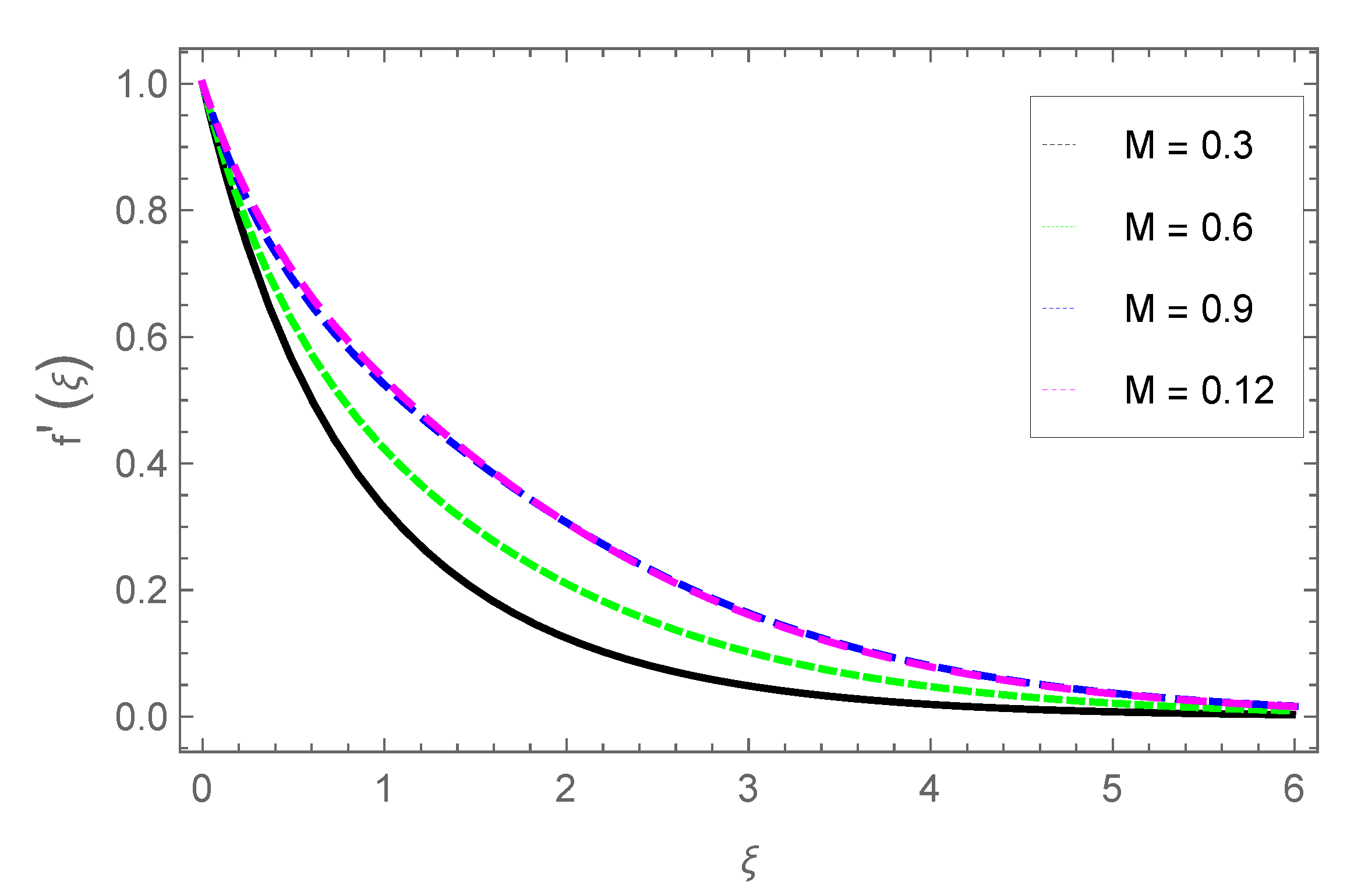
Figure 9.
The against .
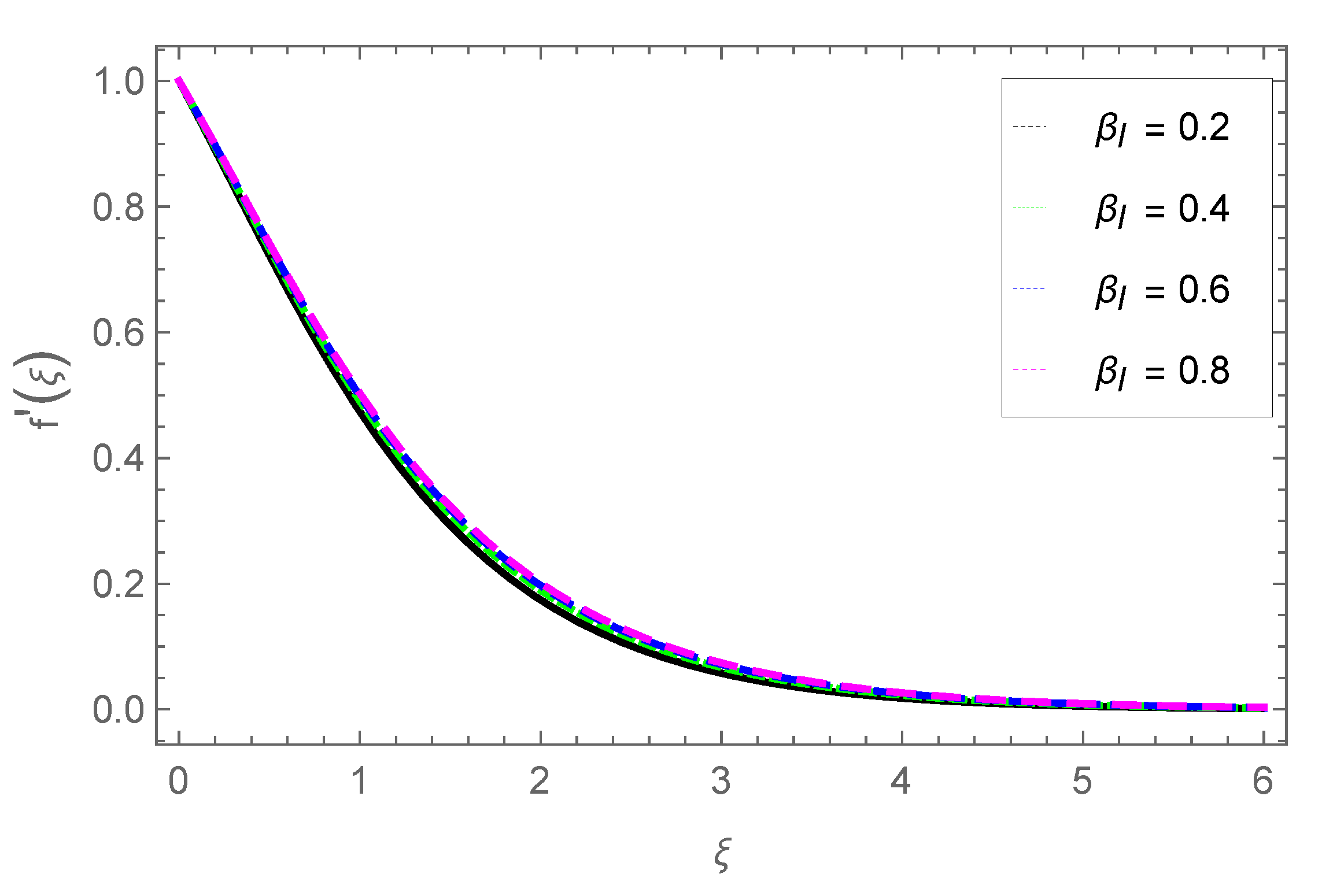
Figure 10.
The against .
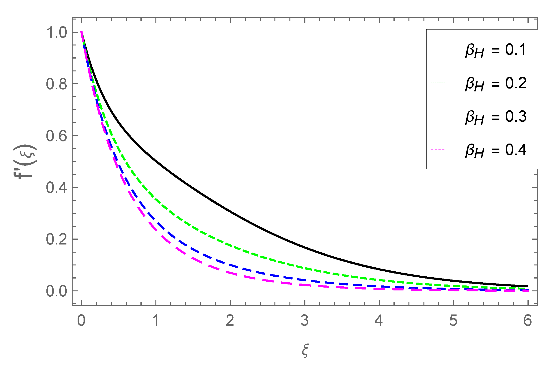
Figure 11.
The against d2.
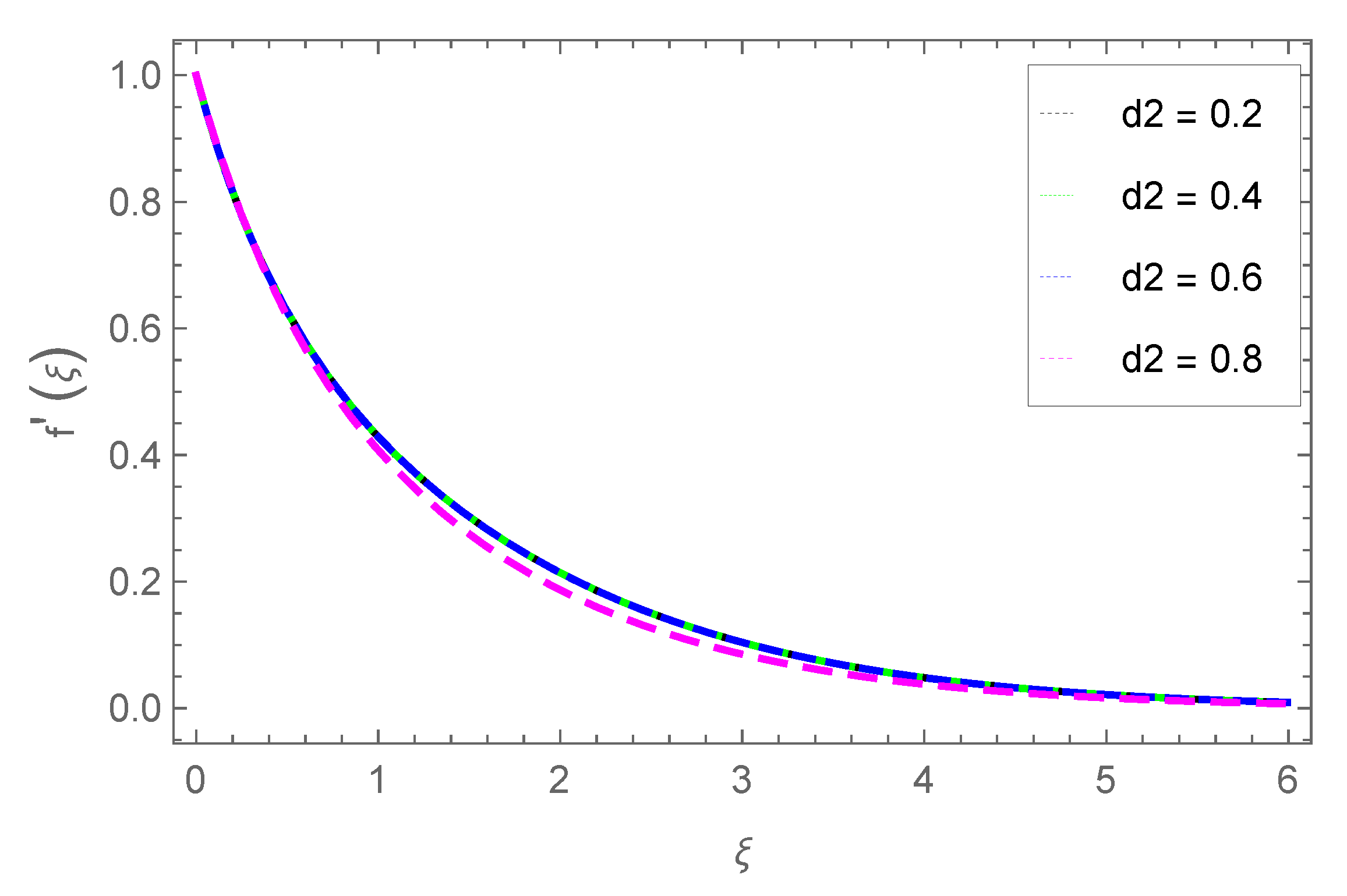
Figure 12.
The against .
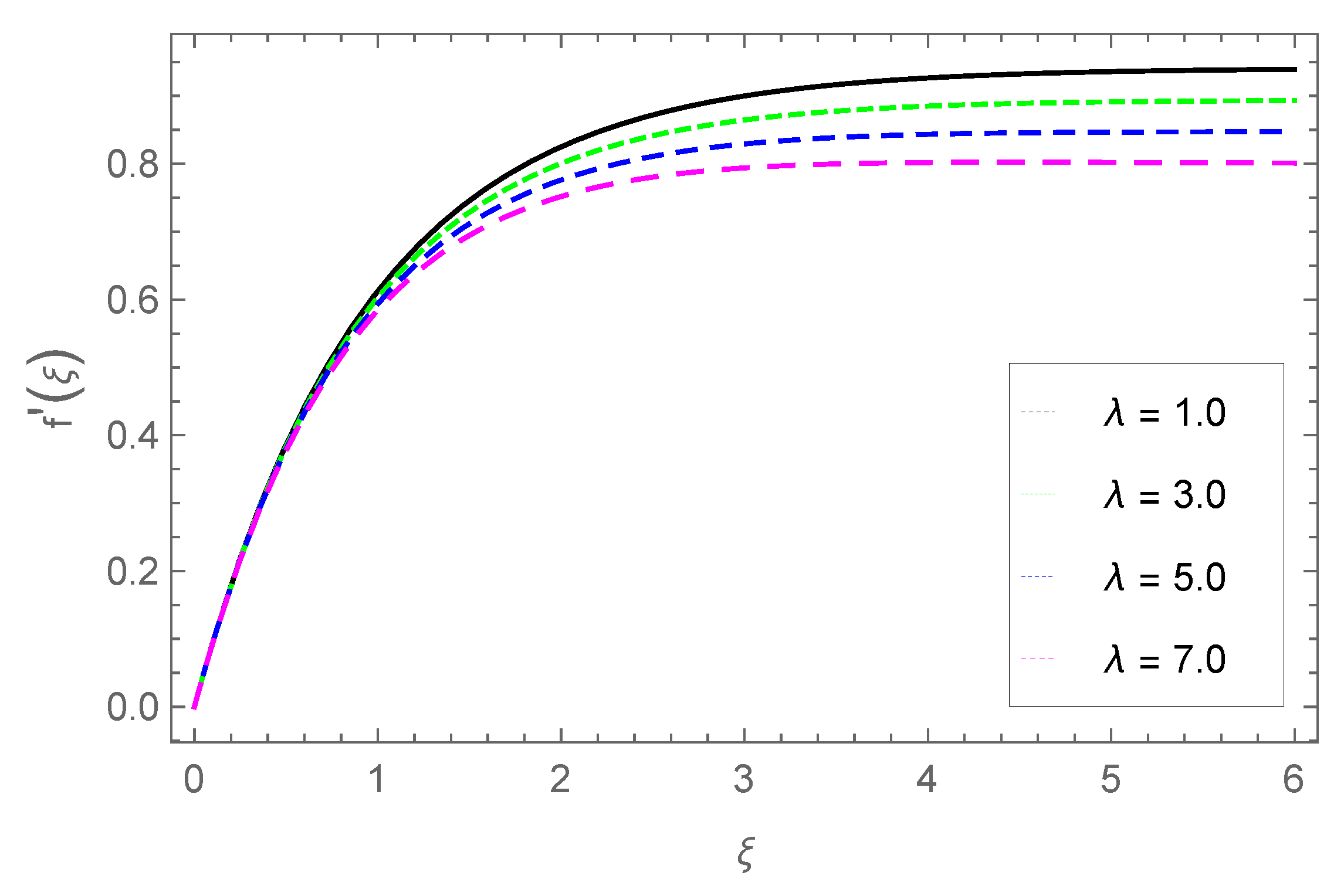
Figure 13.
The against M.
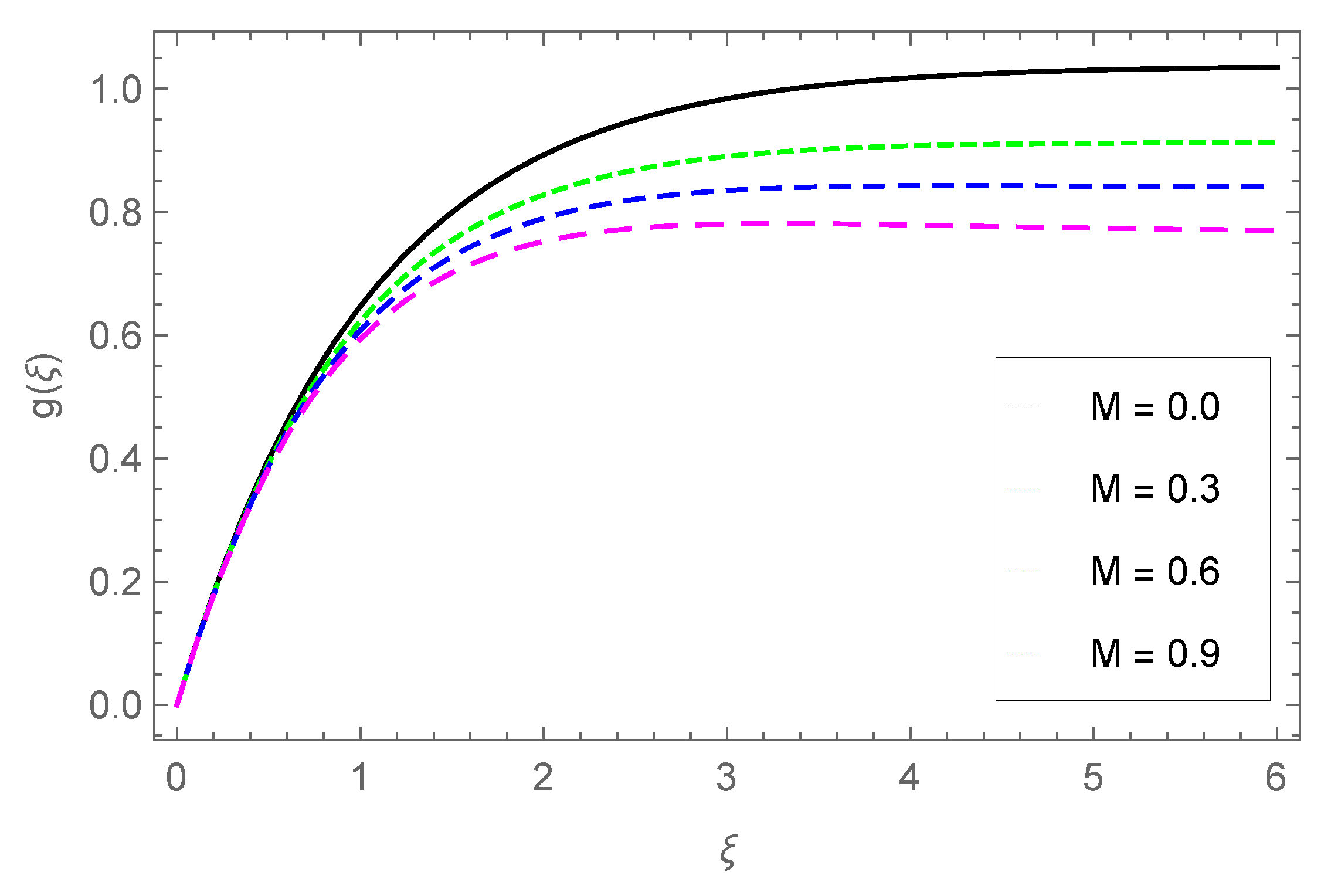
Figure 14.
The against .
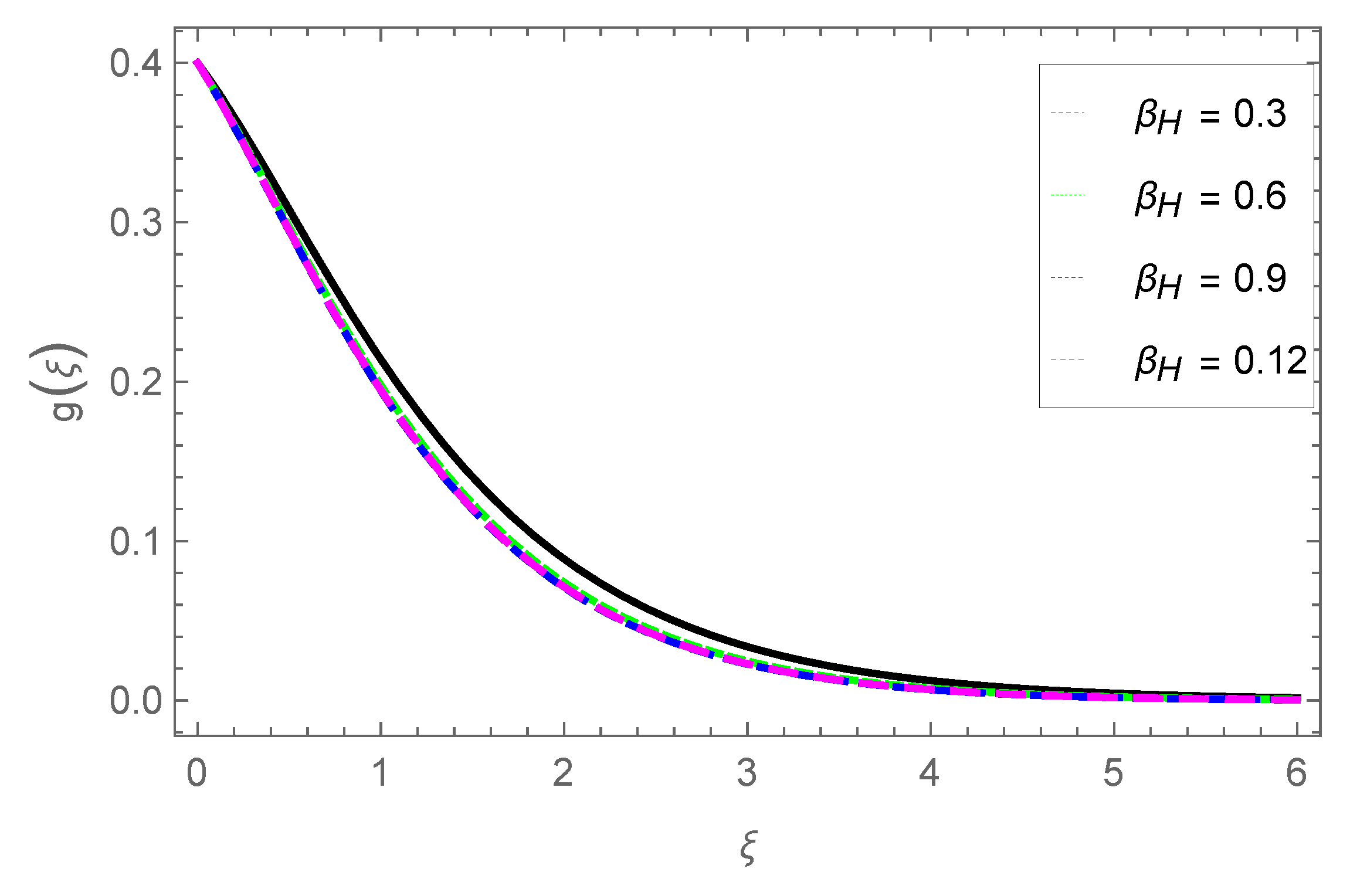
Figure 15.
The against .
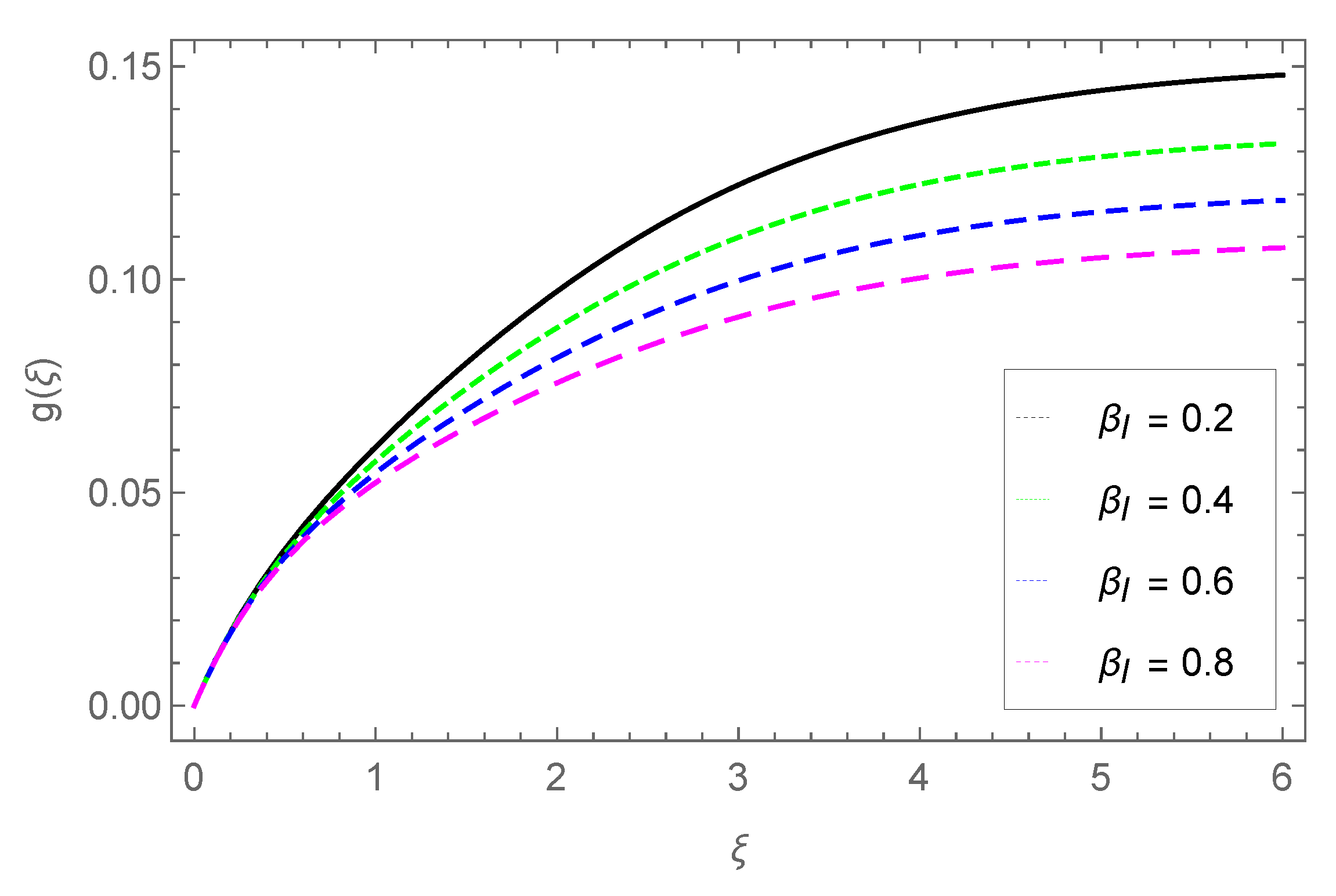
Figure 16.
The against .
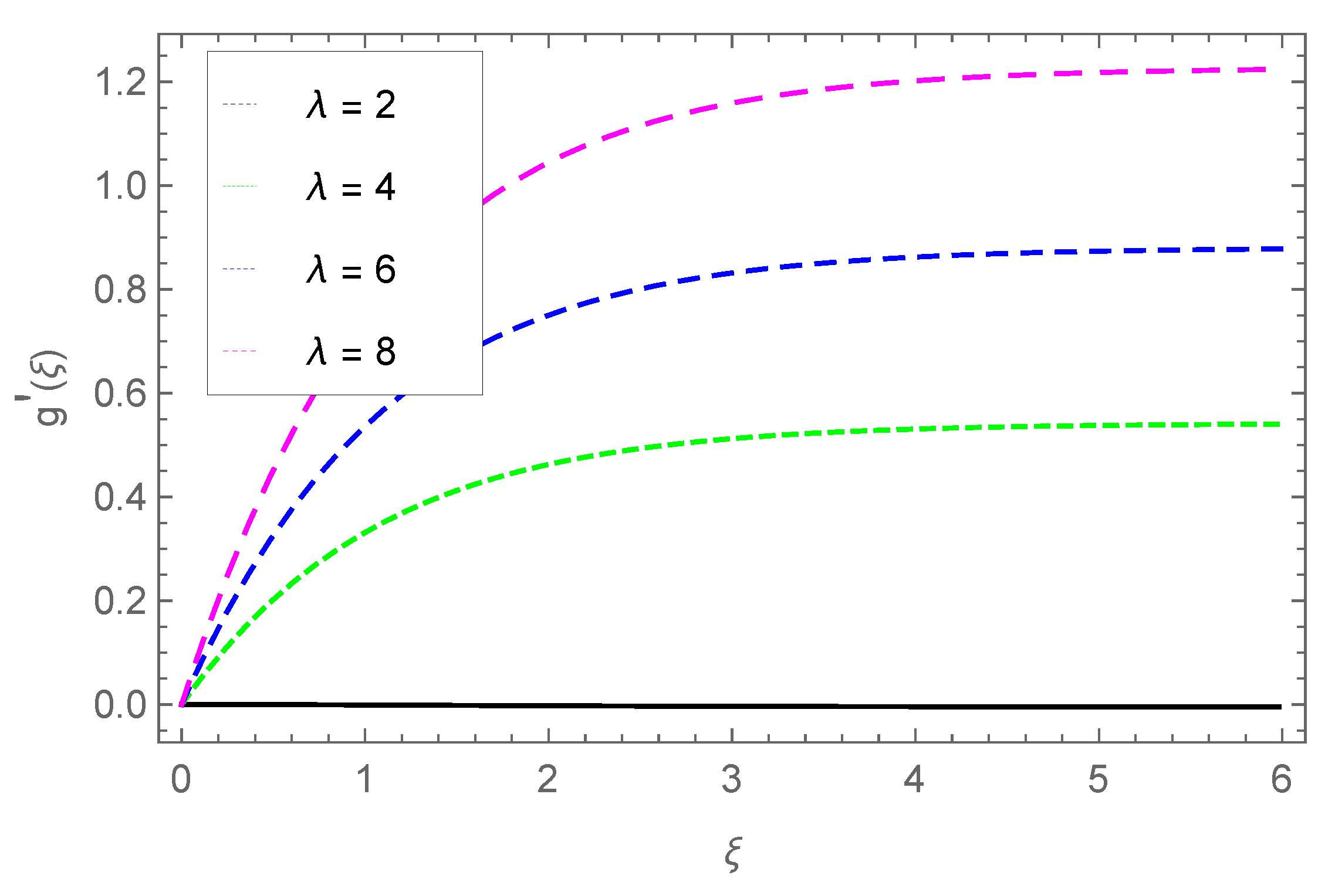
Figure 17.
The against .
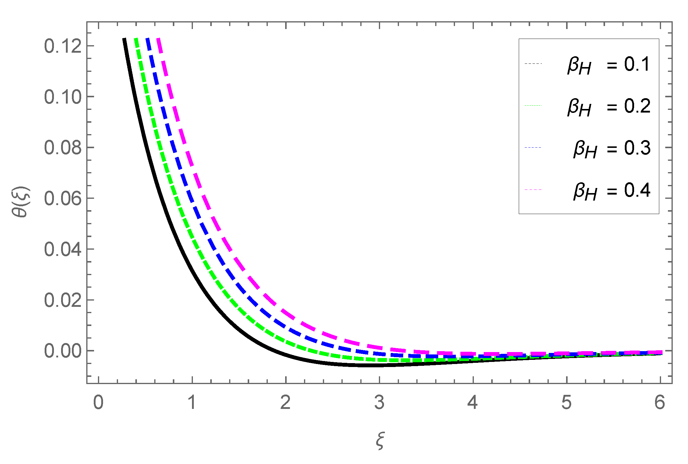
Figure 18.
The against .
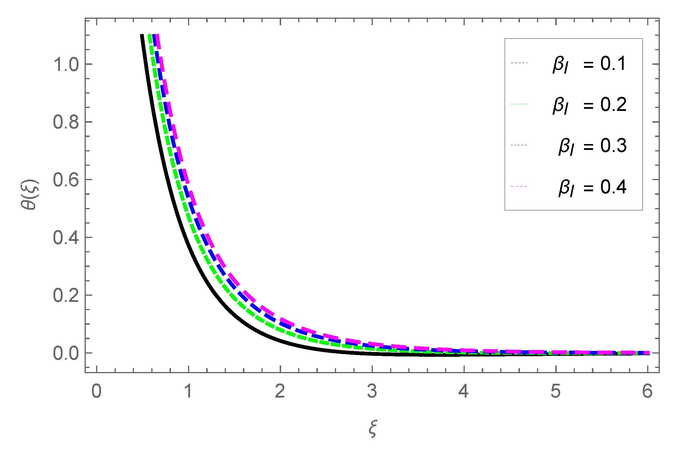
Figure 19.
The against .
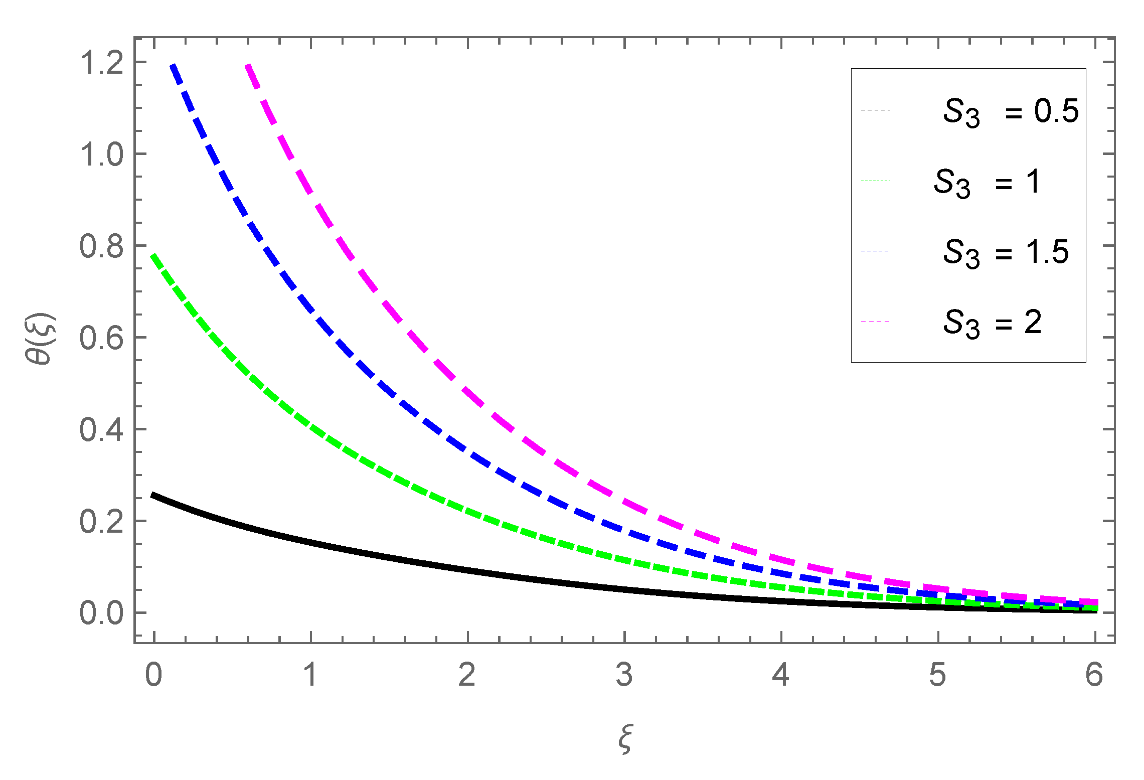
Figure 20.
The against .
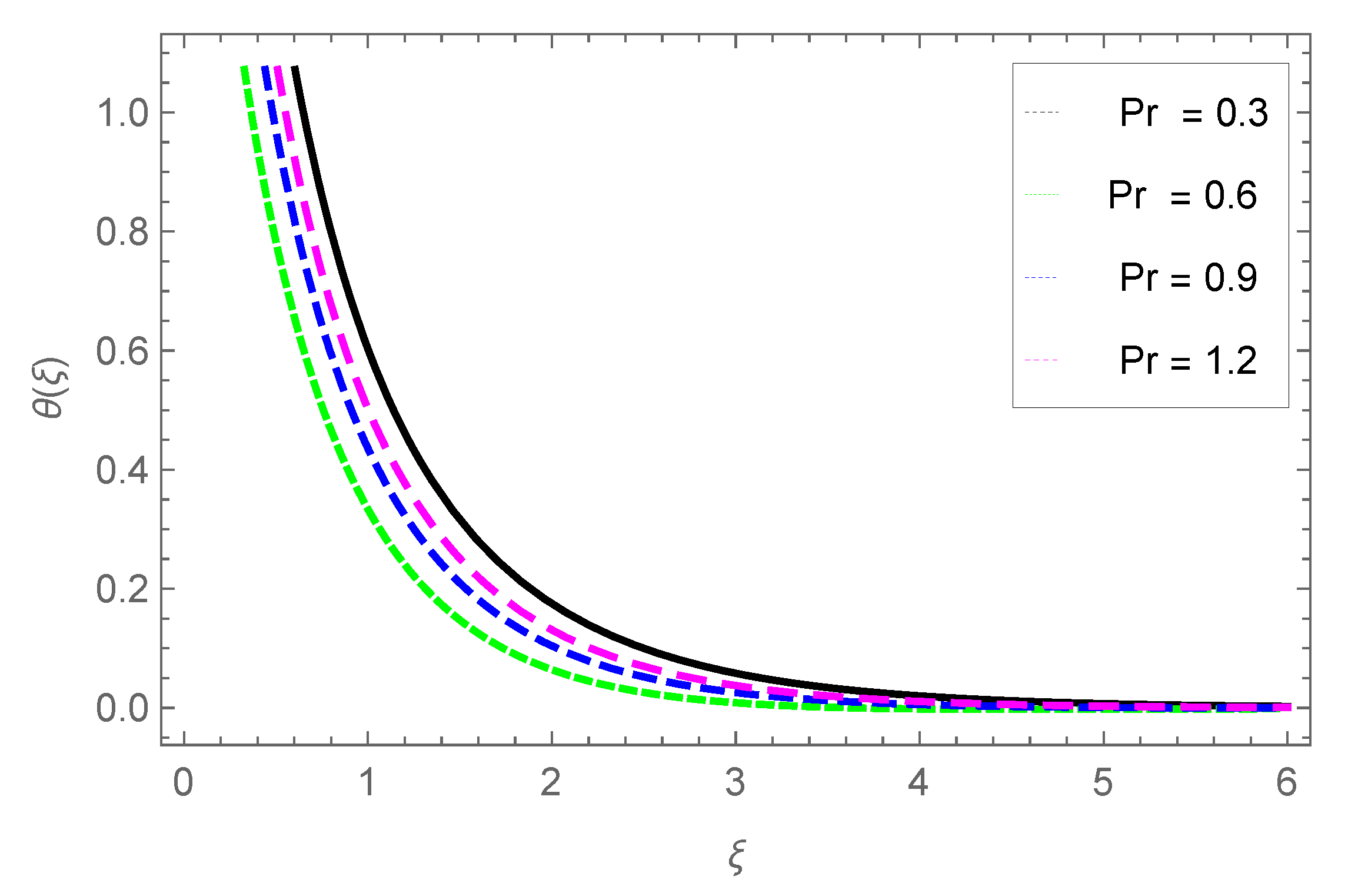
Figure 21.
The against t.
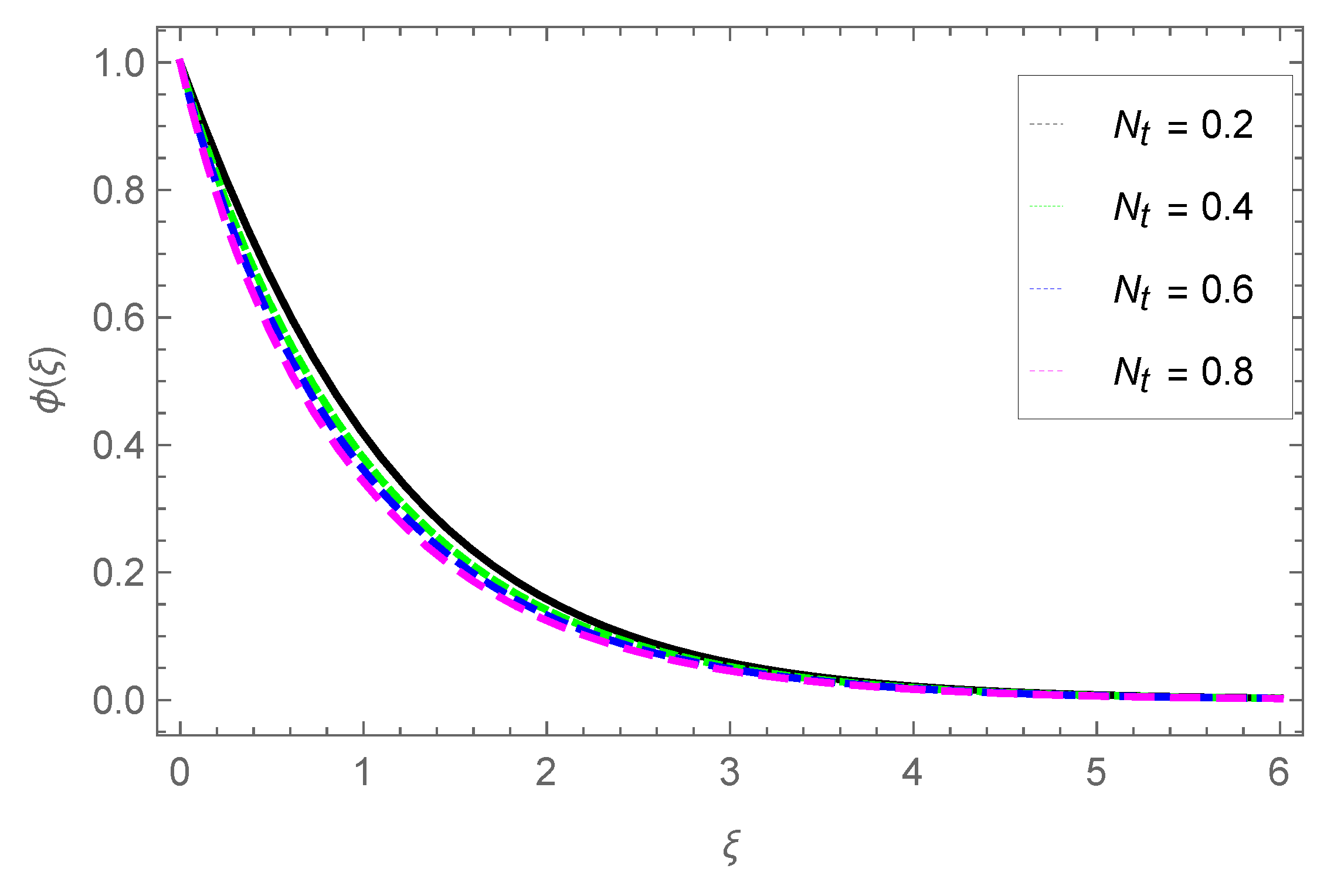
Figure 22.
The against b.
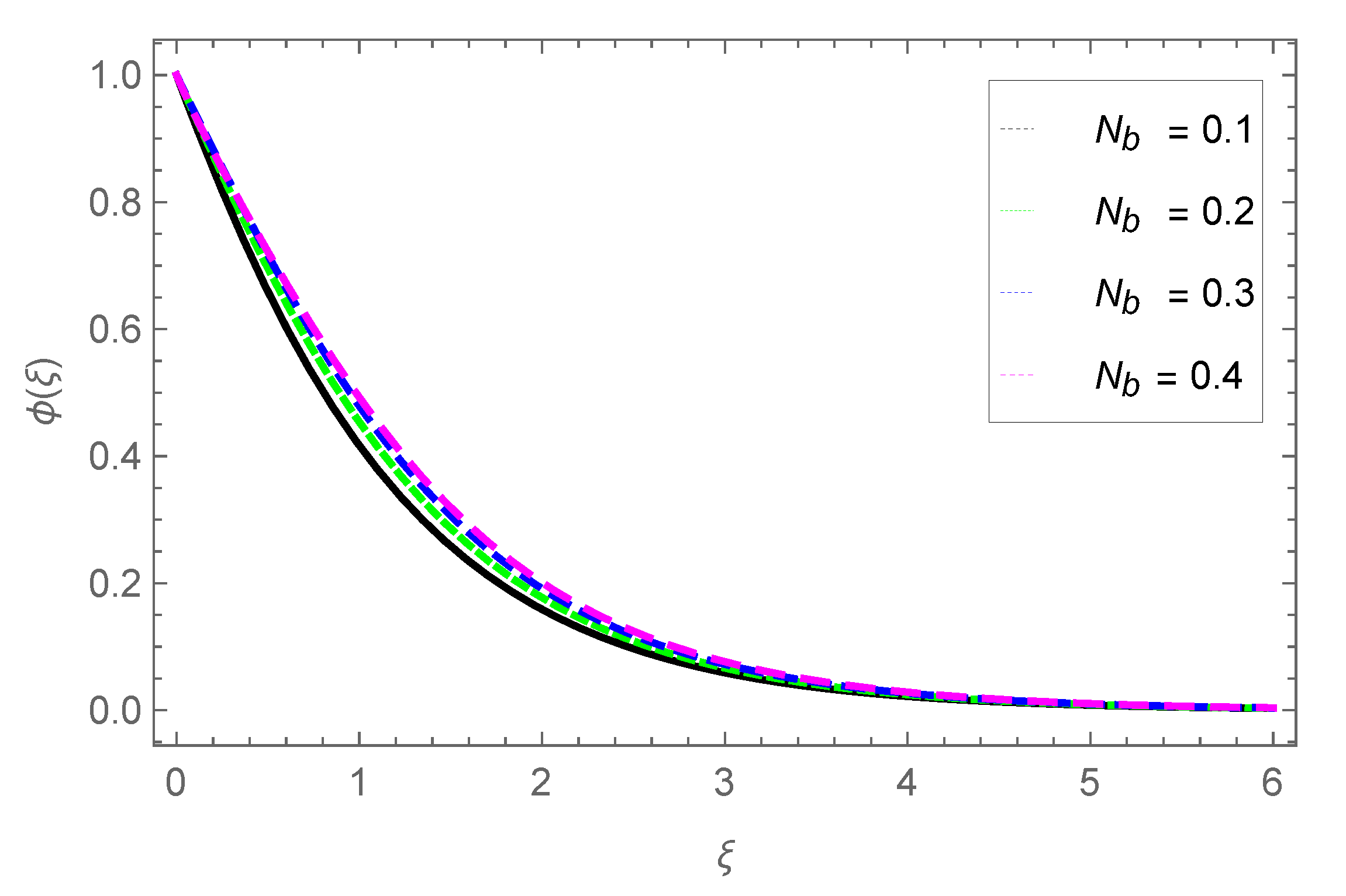
Figure 23.
The against .
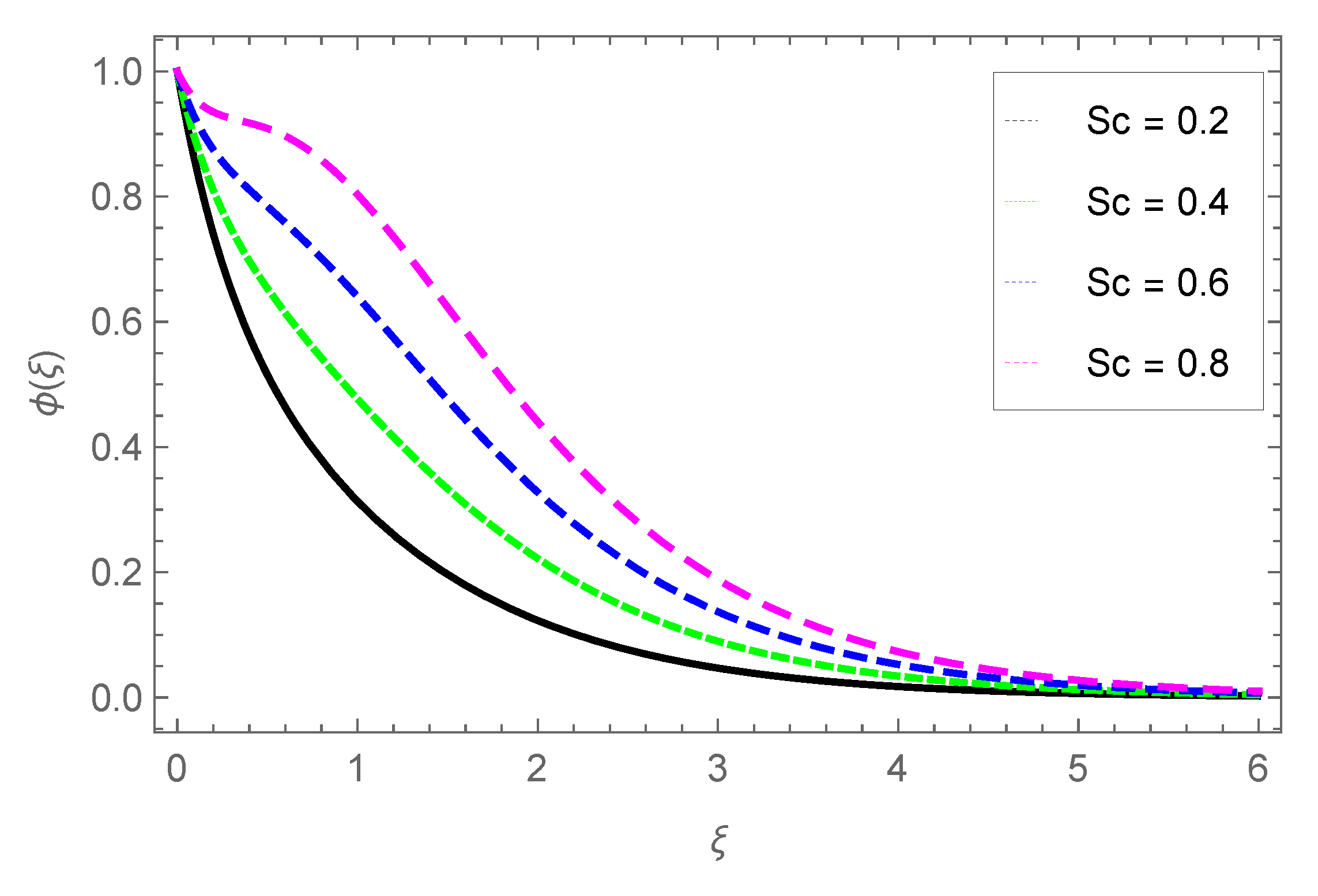
Figure 24.
The against .
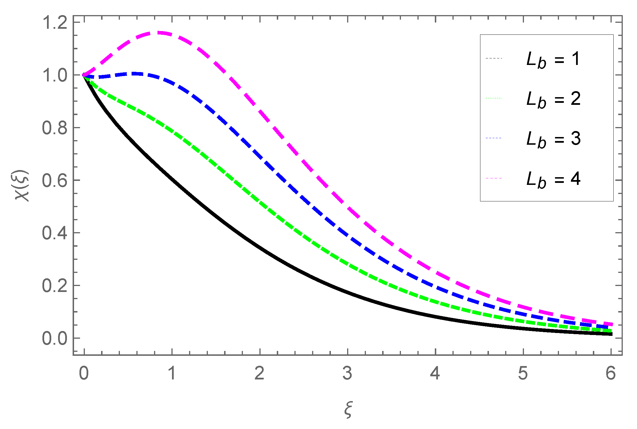
Figure 25.
The against .
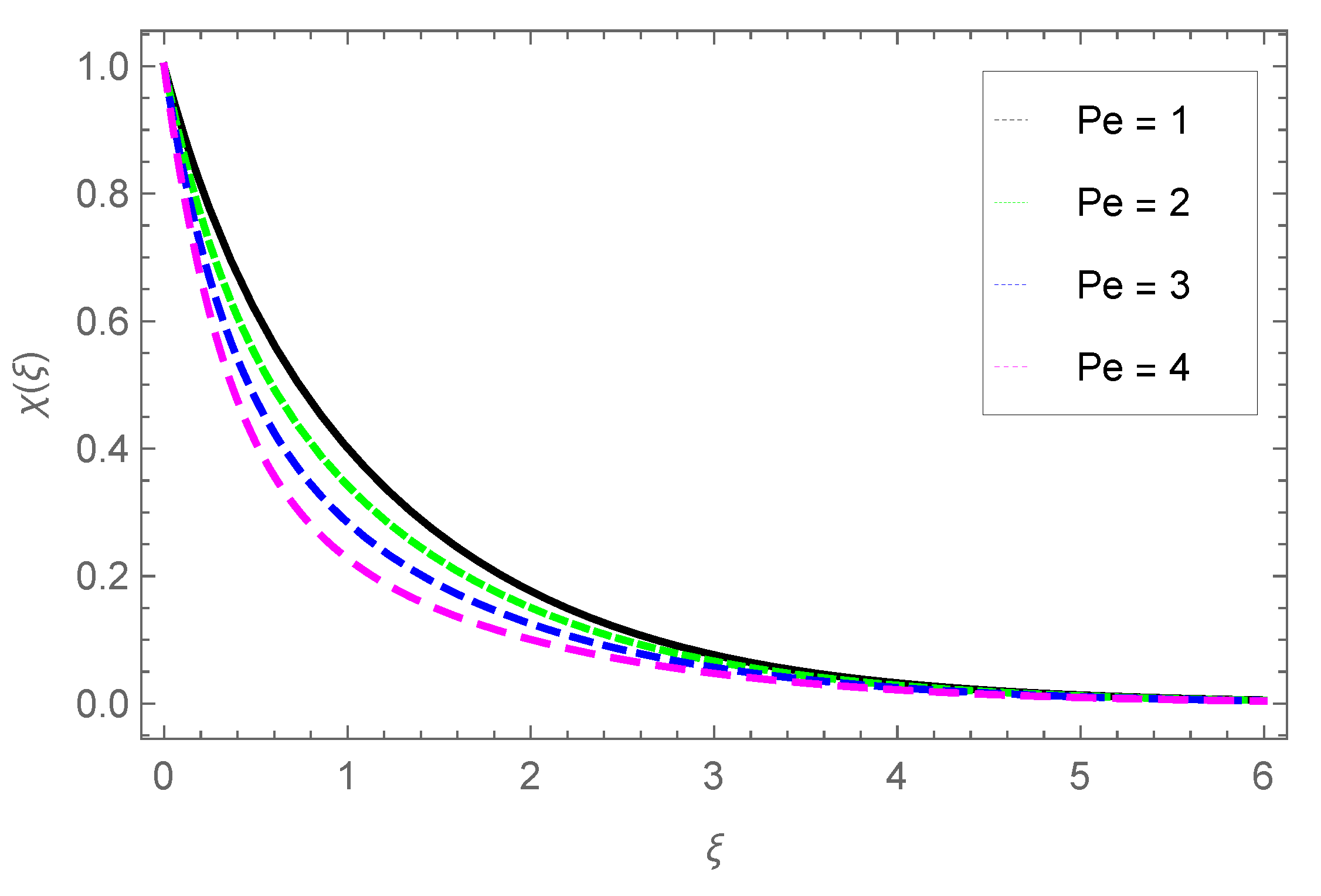
Figure 26.
The against .
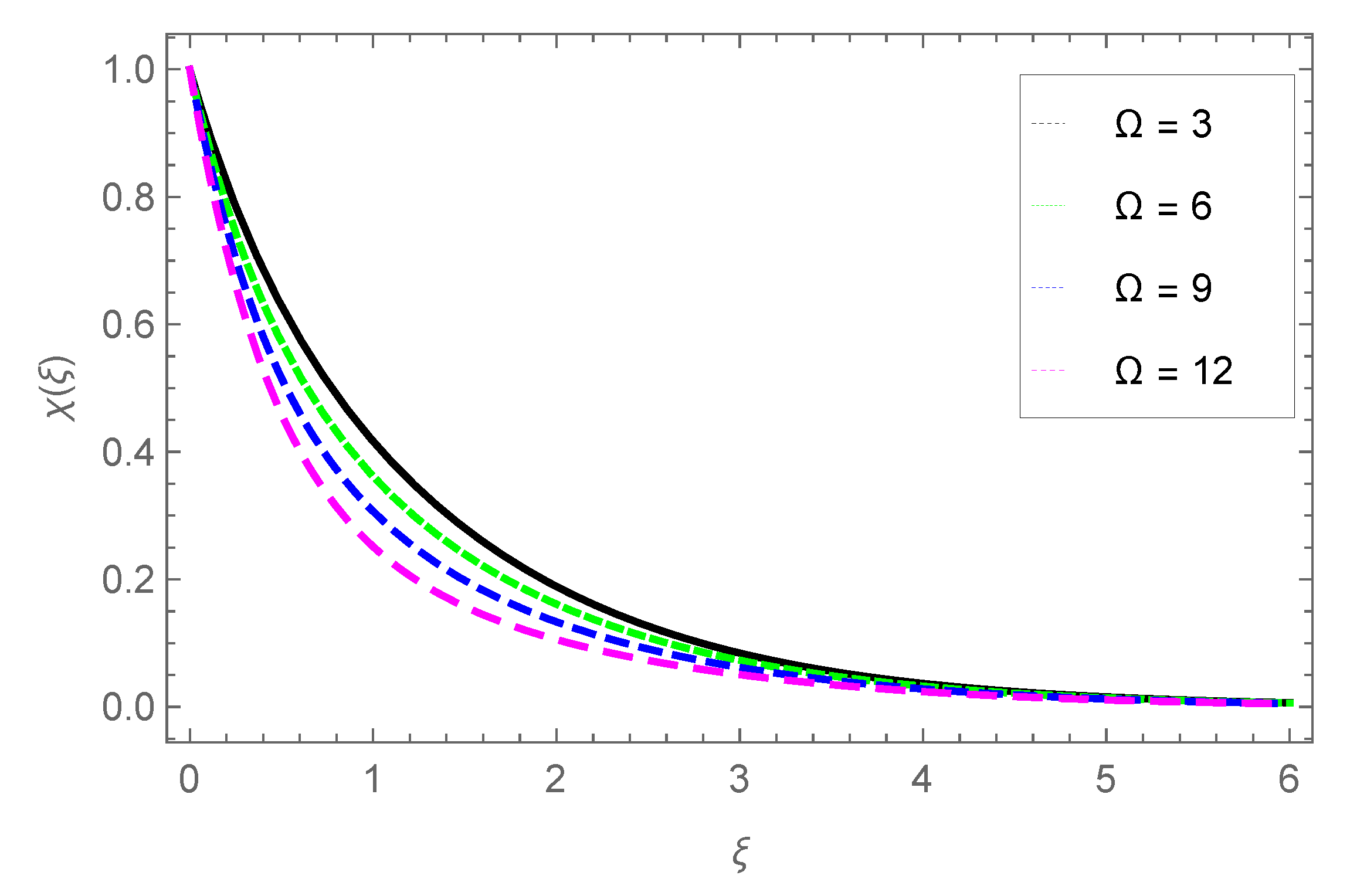

Table 1.
Performance of influence , , on the Nuselt number .
| M | [37] | Present results | ||
|---|---|---|---|---|
| 0.1 | 1 | 0.2 | 0.852219 | 0.852218 |
| 0.1 | 1.5 | 0.3 | 0.870754 | 0.870752 |
| 0.1 | 2 | 0.4 | 0.884226 | 0.884224 |
| 0.1 | 2.5 | 0.5 | 0.890434 | 0.890432 |
| 0.2 | 0.2 | 0.1 | 0.889218 | 0.889219 |
| 0.2 | 0.2 | 0.1 | 0.902486 | 0.902485 |
| 0.2 | 0.2 | 0.1 | 0.904523 | 0.904520 |
| 0.2 | 0.2 | 0.1 | 0.906588 | 0.906586 |
| 0.3 | 0.1 | 0.2 | 0.964238 | 0.964235 |
| 0.3 | 0.1 | 0.3 | 1.010009 | 1.010006 |
| 0.3 | 0.1 | 0.4 | 1.115522 | 1.115520 |
| 0.3 | 0.1 | 0.5 | 1.221035 | 1.221033 |
| 0.4 | 0.1 | 0.1 | 0.72467 | 0.72464 |
| 0.4 | 0.1 | 0.1 | 0.878117 | 0.878116 |
| 0.4 | 0.1 | 0.1 | 0.891306 | 0.891307 |
| 0.4 | 0.1 | 0.1 | 0.904496 | 0.904494 |
Table 2.
Performance of the skin friction coefficients and to show the comparison with published work.
Table 2.
Performance of the skin friction coefficients and to show the comparison with published work.
| [37] | [36] | Present results | [37] | [36] | Present results |
|---|---|---|---|---|---|
| 0.719070243 | 0.719070241 | 0.719070240 | 0.111575838 | 0.111575831 | 0.111575830 |
| 0.757387985 | 0.757387982 | 0.757387980 | 0.281564212 | 0.281564212 | 0.281564211 |
| 0.797424135 | 0.797424132 | 0.797424131 | 0.394505727 | 0.394505723 | 0.394505722 |
| 0.823405641 | 0.823405643 | 0.823405642 | 0.451557772 | 0.451557774 | 0.451557772 |
| 0.887549495 | 0.887549494 | 0.887549492 | 0.564039884 | 0.564039884 | 0.564039883 |
| 0.887549495 | 0.887549496 | 0.887549495 | 0.55719186 | 0.55719181 | 0.55719182 |
| 0.887549495 | 0.887549497 | 0.887549496 | 0.55719186 | 0.55719182 | 0.55719181 |
| 0.887549595 | 0.887549598 | 0.887549597 | 0.55719186 | 0.55719183 | 0.55719182 |
| 0.887549495 | 0.887549491 | 0.887549490 | 0.564039884 | 0.564039884 | 0.564039882 |
| 0.887044175 | 0.887044172 | 0.887044171 | 0.564039884 | 0.564039885 | 0.564039883 |
| 0.887044175 | 0.887044173 | 0.887044172 | 0.564039884 | 0.564039886 | 0.564039885 |
| 0.887044175 | 0.887044174 | 0.887044174 | 0.564039884 | 0.564039887 | 0.564039884 |
| 0.887044175 | 0.887044175 | 0.887044174 | 0.234080623 | 0.234080628 | 0.234080627 |
| 0.745831925 | 0.745831925 | 0.745831923 | 0.226862343 | 0.226862341 | 0.226862340 |
| 0.741235004 | 0.741235004 | 0.741235002 | 0.224322014 | 0.224322012 | 0.224322011 |
| 0.736437806 | 0.736437806 | 0.736437804 | 0.222927008 | 0.222927005 | 0.222927004 |
| 0.731437806 | 0.731437806 | 0.731437805 | 0.221986349 | 0.221986346 | 0.221986345 |
| 0.726117576 | 0.726117576 | 0.726117575 | 0.664419328 | 0.664419327 | 0.664419326 |
| 0.80225148 | 0.80225148 | 0.80225147 | 0.671397457 | 0.671397456 | 0.671397455 |
| 0.981391226 | 0.981391226 | 0.981391225 | 0.765839488 | 0.765839488 | 0.765839487 |
| 1.158190169 | 1.158190169 | 1.158190168 | 0.947744044 | 0.947744044 | 0.947744043 |
| 1.476161533 | 1.476161533 | 1.476161531 | 1.153120999 | 1.153120999 | 1.153120998 |
| 1.839517997 | 1.839517997 | 1.839517996 | 0.679775184 | 0.679775184 | 0.679775183 |
| 0.993626652 | 0.993626652 | 0.993626651 | 0.655608013 | 0.655608013 | 0.655608012 |
| 0.884899639 | 0.884899639 | 0.884899638 | 0.612787646 | 0.612787646 | 0.612787645 |
| 0.802264361 | 0.802264361 | 0.802264360 | 0.563176151 | 0.563176151 | 0.563176150 |
| 0.748580802 | 0.748580802 | 0.748580800 | 0.513618696 | 0.513618696 | 0.513618695 |
| 0.716979363 | 0.716979363 | 0.716979362 | 0.656965055 | 0.656965055 | 0.656965054 |
| 0.661008802 | 0.661008802 | 0.661008801 | 0.555527812 | 0.555527812 | 0.555527811 |
| 0.74256172 | 0.74256172 | 0.74256170 | 0.455495507 | 0.455495507 | 0.455495506 |
| 0.77837091 | 0.77837091 | 0.77837090 | 0.386043017 | 0.386043017 | 0.386043016 |
| 0.785950317 | 0.785950317 | 0.785950316 | 0.337580336 | 0.337580336 | 0.337580335 |
| 0.784265665 | 0.784265665 | 0.784265664 | 0.556669165 | 0.556669165 | 0.556669163 |
| 0.856524973 | 0.856524973 | 0.856524972 | 0.556669165 | 0.556669165 | 0.556669164 |
| 0.856524973 | 0.856524973 | 0.856524972 | 0.556669165 | 0.556669165 | 0.556669162 |
| 0.856524973 | 0.856524973 | 0.856524971 | 0.556669165 | 0.556669165 | 0.556669163 |
| 0.856524973 | 0.856524973 | 0.856524972 | 0.556669165 | 0.556669165 | 0.556669163 |
| 0.856524973 | 0.856524973 | 0.856524972 | 0.556669165 | 0.556669165 | 0.556669164 |
| 0.856524973 | 0.856524973 | 0.856524971 | 0.556669165 | 0.556669165 | 0.556669164 |
Table 3.
The efficiency is displayed in relation to work that has been released.
| [37] | [36] | Present results |
|---|---|---|
| 1.5990239 | 1.5990231 | 1.5990231 |
| 1.4202682 | 1.4202682 | 1.4202682 |
| 1.1564338 | 1.1564333 | 1.1564333 |
| 0.9287895 | 0.9287894 | 0.9287894 |
| 0.5494868 | 0.5494865 | 0.5494865 |
| 0.8096016 | 0.8096016 | 0.8096016 |
| 1.0905005 | 1.0905007 | 1.0905007 |
| 1.3286006 | 1.3286008 | 1.3286008 |
| 0.5491808 | 0.5491809 | 0.5491809 |
| 0.9287895 | 0.9287895 | 0.9287895 |
| 1.2669854 | 1.2669854 | 1.2669854 |
| 1.3689696 | 1.3689696 | 1.3689696 |
| 1.4844171 | 1.4844171 | 1.4844171 |
| 1.4833107 | 1.4833107 | 1.4833107 |
| 1.4821196 | 1.4821196 | 1.4821196 |
| 1.4808276 | 1.4808276 | 1.4808276 |
| 1.4794173 | 1.4794173 | 1.4794173 |
| 0.9433476 | 0.9433476 | 0.9433476 |
| 0.910217 | 0.910217 | 0.910217 |
| 0.8077522 | 0.8077522 | 0.8077522 |
| 0.7457675 | 0.7457675 | 0.7457675 |
| 0.1187274 | 0.1187274 | 0.1187274 |
| 0.4541371 | 0.4541371 | 0.4541371 |
| 0.8618128 | 0.8618128 | 0.8618128 |
| 1.1292928 | 1.1292928 | 1.1292928 |
| 1.2931189 | 1.2931189 | 1.2931189 |
| 0.9552824 | 0.9552824 | 0.9552824 |
| 1.159594 | 1.159594 | 1.159594 |
| 1.3236266 | 1.3236266 | 1.3236266 |
| 1.4156669 | 1.4156669 | 1.4156669 |
| 1.4692599 | 1.4692599 | 1.4692599 |
| 0.66944612 | 0.66944612 | 0.66944612 |
| 0.8129271 | 0.8129271 | 0.8129271 |
| 0.8957033 | 0.8957033 | 0.8957033 |
| 0.9287895 | 0.9287895 | 0.9287895 |
| 0.94665 | 0.94665 | 0.94665 |
| 0.946555 | 0.946555 | 0.946555 |
| 0.8129271 | 0.8129271 | 0.8129271 |
Disclaimer/Publisher’s Note: The statements, opinions and data contained in all publications are solely those of the individual author(s) and contributor(s) and not of MDPI and/or the editor(s). MDPI and/or the editor(s) disclaim responsibility for any injury to people or property resulting from any ideas, methods, instructions or products referred to in the content. |
© 2025 by the authors. Licensee MDPI, Basel, Switzerland. This article is an open access article distributed under the terms and conditions of the Creative Commons Attribution (CC BY) license (http://creativecommons.org/licenses/by/4.0/).
Copyright: This open access article is published under a Creative Commons CC BY 4.0 license, which permit the free download, distribution, and reuse, provided that the author and preprint are cited in any reuse.


