
Submitted:
19 April 2025
Posted:
21 April 2025
You are already at the latest version
Abstract
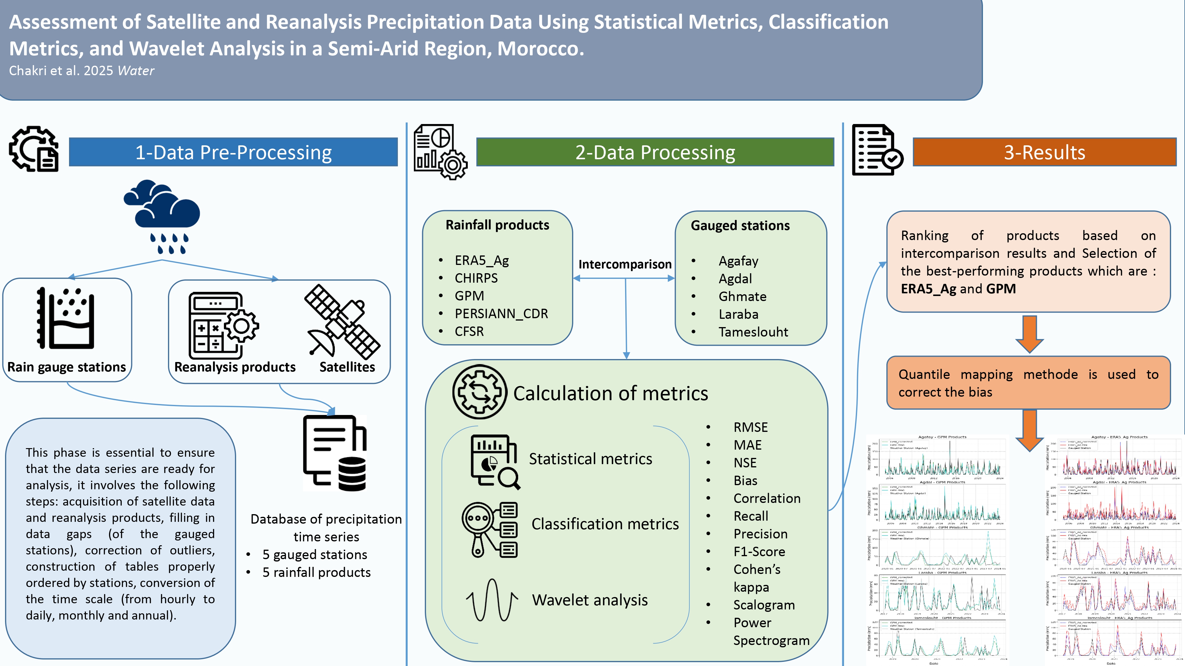
Climate change, marked by decreasing rainfall and increasing extreme events, represents a major challenge for water resources, particularly in semi-arid regions. To estimate aquifer recharge, it is essential to assess the fraction of precipitation contributing to groundwater recharge and to implement a water balance model. However, the limited number of rainfall stations has led researchers to rely on satellite and reanalysis rainfall products. The accuracy of these datasets is essential for reliable hydrological modeling. In this study, we evaluated five rainfall products—CHIRPS, ERA5_Ag, CFSR, GPM, and PERSIANN-CDR—by comparing them to ground measurements from gauging stations in the central Haouz region of Marrakech at three temporal scales: daily, monthly, and annual. Statistical and classification measures were applied, as well as wavelet analysis, to improve the accuracy of the evaluation. The results identified ERA5_Ag and GPM as the most accurate products in capturing rainfall events. Nevertheless, ERA5_Ag showed a high bias. After applying the quantile mapping method to correct the bias, the product exhibited greater accuracy. The corrected datasets from these two products will be used to estimate recharge over the last 30 years, contributing to the development of a hydrogeological model for groundwater dynamics.
Keywords:
rainfall products
; statistical metrics
; wavelet analysis
; bias correcti
; classification 17 metrics
; gauged stations
1. Introduction
Intercomparison of satellite products and climate precipitation models with measured data from weather stations is a discipline that has been carried out by many researchers around the world, in order to validate the contribution of remote sensing and improve the quality of data from both satellites and climate models. As in the 1990’s, intercomparison studies of precipitation products [1,2,3,4,5] have revealed an improvement of accuracy in the estimation of precipitation (satellites and climate models), with the aim of enhancing and developing the algorithms of climate models. Studies comparing satellite products with measured data have already been initiated in Africa, demonstrating perfect agreement between them [6,7,8]. The main objective of this comparison lies in the fact that the limited number of meteorological stations makes the spatialization of precipitation over large areas less effective. This spatialization process is essential for generating raster datasets used as inputs for hydrological models and climate indices calculations [9,10,11,12]. It has to be noted that each data source has its own performance level in providing climate variables, depending on the primary data used. These may come from direct satellite observations [13,14] or from algorithms based on multi-source satellite data interpretation [15,16,17]. The climate context of the study area can affect the performance of these data sources. For instance, a satellite product may perform well in a temperate climate but be less reliable in an arid region. Several studies have explored these discrepancies; for example, [18,19] examined the TRMM satellite and concluded that satellite based products tend to be more accurate in tropical regions but less precise in arid, mountainous, or highly variable precipitation zones. Similarly, studies of [20,21,22] indicate that satellite products often struggle to estimate precipitation accurately in mountainous regions due to complex orographic effects. Likewise, in arid and semi-arid regions, reanalysis products such as ERA5 and MERRA-2 tend to underestimate precipitation, as they have difficulty in capturing local and sporadic events. The selected product from this study must perform well across three key evaluation tests. The first test involves statistical comparison metrics, including Root Mean Square Error (RMSE), Mean Absolute Error (MAE), Nash-Sutcliffe Efficiency (NSE), Bias, and Pearson correlation. The second test applies classification metrics and wavelet analysis to assess the products ability in capturing precipitation variability. The best performing product will be selected for use in estimating diffuse recharge and building a water balance model of the study area, which is the aim of the next article.
2. Study Area
The area of interest in this study is an alluvial plain, bordered to the South by the High Atlas mountains, to the North by the Jbilettes, and bounded by Oued N’Fis to the West and Oued Rhdate to the East. Figure 1 shows its geographical location, which is situated between 31° and 32° North latitude and 7° and 9° West longitude.
The Haouz plain is generally dry, due to high average temperatures (reaching 40°C) and intense evaporation. The four months from June to September constitute the dry season, with around 10 mm of precipitation per month. While precipitations is distributed throughout the year, most of it falls between October and May, varying between 25 and 65 mm per month. Annual precipitation ranges from 220 to 800 mm, with an average of approximately 415 mm, based on data from 1973 to 2009 (September to August). The region has a semi-arid continental climate.
3. Materials and Methods
The comparison is based on analysis at the pixel-point scale, relatively linked to the location of the meteorological measurement stations. The latters are irregularly distributed in the region, adding their limited number and the mismatch between the launch dates of each station, showing a well-defined contrast, ranging from 2003 to 2019 with a gap of 16 years, which complicates the analyses. The raw precipitation data from gauged stations have 30 min time step,requiring transformation to a daily, monthly and annual time scale. The transformation is the sum of the values recorded at a time step of 30 min. The satellite data have a daily, monthly and annual time step, enabling statistical intercomparison analyses. For satellite data extraction, we adopt the proximity criterion, selecting the pixel value that coincides with or is closest to the geographical position of the weather station. Statistical tests are conducted over different time period from each station to another, due to their different commencement dates. Multiscale tests are applied while considering the variability and magnitude of the time scales (daily, monthly and annual). The range of data chosen for comparison tests has no gaps in the recordings, making the analyses more reliable and representative.
3.1. Characteristics of Rainfall Products and Gauged Stations
Each meteorological station is presented by its geographical coordinates, altitude, date of first start-up, parameters measured and frequency of measurement, see Table 1. The present study took five automatic measuring stations belonging to LMI TREMA [23], which are well distributed geographically across the study area. Given the proximity of the Graoua and Agdal stations, we choose to use data from the Agdal station, which offers better data quality. Similarly, for the Laraba and Saada stations, we selected Laraba because of its longer measurement period than Saada. Thus, the weather stations selected provide representative, spatially well distributed data that are sufficient for intercomparison studies.
For satellite and reanalysis products, the value is assigned to the pixel corresponding to the spatial location of the measuring station. Satellite data cover several spatial and temporal scales, Table 2 lists the characteristics of each satellite and reanalysis product used for precipitation estimates.
3.2. Statistical metrics
Assessing the robustness of satellite and reanalyzed precipitation products by comparing them with meteorological stations measurements is an approach adopted by several authors [24,25,26,27,28,29,30]. Statistical measures are used to evaluate satellite and reanalysis datasets by analyzing estimation errors in relation to gauged station measurements. The principal metrics employed to assess the performance of satellite and reanalysis products in estimating precipitation are presented in Table 3.
The root-mean-square (RMSE) metric is used to assess the dispersion between measured and estimated values, and provides an overview of the ability of models (in our case, satellites and reanalysis products) to provide estimates of variables that are closer to in situ measurements. Several studies have employed this parameter to assess model outputs and quantify the differences between simulated and observed data [31,32,33,34].
Systematic errors and deviations in measurements or estimations are quantified by Bias. The output of a model is biased when it differs from the actual values. A high bias indicates the model’s weakness in capturing the complexity of the data, while a low bias indicates that the model provides fewer errors and that the outputs are closely matched to the real data. The relationship between Bias and variance must be considered into account when validating a model, as the balance between these two parameters is essential if the model is to be accurate and reliable. In general, a low Bias produces accurate outputs, while a low variance provides consistent outputs. The value of Bias ranges between the infinite interval (-∞,+ ∞), with a value of 0 indicating complete agreement between measured and estimated values.
The Pearson R correlation index, commonly used by researchers in many fields [16,35,36,37,38,39,40] , is a statistical measure that quantifies the linear relationship between two variables and assesses the degree of interdependence between them. This index is used to assess the linear fit of precipitation between satellite products and weather stations. Pearson’s R coefficient is the product of dividing the covariance of the two variables by the product of their standard deviations. The value of R lies between the interval -1 and 1. Values below 0 indicate that the relationship between the variables is negative, i.e. if variable X increases, variable Y decreases, and vice-versa; an R coefficient of zero indicates that there is no linear relationship between the two variables. In terms of interpretation, a correlation does not indicate a causality, but rather signifies a concrete statistical relationship. On the other hand, a hidden common factor may influence both variables, creating the causal relationship.
3.3. Classification Metrics and Wavelet Analysis
The intercomparison of satellite and reanalyzed products is improved by the application of other statistical measures, such as classification metrics. Detailed visualization of each product’s performance is explored through the confusion matrix. By definition, this matrix is a table showing the true and false predictions for each class. The calculation of classification metrics depends on this matrix. For a binary classification problem (rainy day or dry day), the shape of the matrix is shown in Table 4. The classification threshold is an important criterion that should be defined when calculating the matrix. This threshold defines the minimum amount of precipitation from which such a day is considered as rainy, for the case of the present study, we have defined a threshold of 1 mm, by which all days with precipitation greater than or equal to 1 mm will be classified as a rainy day, while for days less than 1 will be classified as dry days.
Classification metrics are derived from the confusion matrix. Accuracy is one of the classification metrics, measuring the percentage of agreement between observed and estimated data, which is aimed to assess the overall reliability of the products. Precision Indicates the proportion of days estimated as rainy which were actually rainy according to the measuring stations. Recall measures the product’s ability to detect all the rainy days recorded by the weather stations. The F1-Score metric is an average between recall and precision, useful for evaluating the overall performance of products. Cohen’s Kappa metric evaluates products by measuring the agreement between estimates and actual values. Table 5 below shows the formulas for calculating these metrics.
Wavelet analysis provides a significant additional value in the study. This approach makes it possible to examine rainfall variations on different time scales. By analyzing the wavelet spectrum of each series, we can identify the dominant periods of observed and estimated precipitation, and see the rainfall event capture performance of each product. The process of applying this method is described as follows ; The first step concerns data preprocessing, which is crucial for ensuring the reliability of the results, and the preparation of data series so that the comparison series must cover the same period and have the same temporal resolution (daily, monthly or yearly). The second step involved the application of wavelet transforms. We chose the Continuous wavelet transform (CWT) to analyze the temporal signals; as opposed to the Fourier method, the CWT decomposes the signal into fixed frequencies, enabling us to analyze the variability of precipitation as a function of frequency and time, thus generating a temporal spectrogram showing the differences in precipitation between stations and satellite products and reanalyzing them.
The mathematical expression of CWT (1) is written as follows :
With : wavelet coefficients associated with scale a and time position b, and
is the Mother wavelet function (2).
The complex Morlet wavelet was selected for the reason that it is better adapted to climatic series. Scales from 1 to 50, on the other hand, enable precipitation cycles to be analyzed at different temporal resolutions. The wavelet parameters used are listed in Table 6 below.
3.4. Application of Quantile Mapping for Bias Correction
The product selected is often biased, which means that direct use of the raw precipitation series may have a negative effect on the hydrological modeling results. The quantile mapping method is used to correct bias in the product’s precipitation series. This method adjusts the distribution of product data to match a reference series (measuring stations) [41,42,43,44]. This technique works by constructing cumulative distribution functions (CDFs) for both datasets (satellite / reanalysis products and weather station data). It then identifies equivalent quantiles in the biased distribution, establishing a correspondence with observations. In concrete terms, each value in the biased data is adjusted according to this correspondence and replaced by a value closer to the observed data. The mathematical expression of the CDFs function is given by formula 3 below:
With representing the biased data, their empirical CDF, and the CDF of the observed data, gives the quantile of the biased data, and adjusts this quantile to the observed data.
4. Results
Plots of the precipitation values measured and those from satellites and reanalysis products gives an idea of the variability of the data in relation to the gauged stations measurements. The data show a cyclical trend, providing information on dry and wet periods [45], There are also peaks distributed irregularly over time, which indicate periods of thunderstorms recorded at the stations [46,47]. We can already observe that precipitation values are both overestimated and underestimated by products. This variability must be quantified by applying the statistical metrics already mentioned. The accuracy of satellite products and climate models depends on the study’s objective, especially for precipitation. For applications like flood modeling, high temporal precision and minimal errors are crucial to ensure reliable hydrological calculations [9]. On the other hand, study focusing on aquifer recharge from rainfall generally operate on an annual time scale. The range of precipitation data provided by the products is practically 20 years long, which is practically large enough to assess their performance.
4.1. Application of Statistical Continuous Metric for Raw Data (Daily, Monthly and Annually)
At the daily scale, mean absolute errors show similar values from one product to another, with a mean value of 0.85. The CHIRPS product shows the highest mean in the 5 stations (MAE = 1.6), while CFSR and GPM show minimal values compared to the other products (0.77 and 0.76). As for RMSE, CHIRPS shows the highest values in all five products (RMSE = 6), while ERA5_Ag shows the lowest (RMSE = 2.5). The other products are evenly distributed. The Nash-Sutcliffe Efficiency (NSE), on the other hand, shows negative trends in several products, while the CHIRPS product still shows significant negative values in all stations, while the ERA5_Ag product shows positive values in all stations with the exception of the Agdal station with a negative value see Figure 2.
On a monthly scale, MAE shows different values from one product to another, with an average value deviation of 17 between the observed and estimated values, the product CHIRPS still shows the highest value in the 5 stations (MAE = 30) while PERSIANN_CDR and GPM show minimal values compared to the other products (10 and 13). As for RMSE, CHIRPS and ERA5_AG show the highest values across all five products (RMSE = 32 and 28, respectively, while the other products are contrasted from station to station, with PERSIANN_CDR showing the lowest values (RMSE = 15 at the Tameslouht station). Nash-Sutcliffe Efficiency (NSE) values contrasted strongly between products, with CHIRPS showing negative trends at all stations except Agafay, while PERSIANN_CDR showed positive values at all stations. The other products show alternating negative and positive values across different stations, see Figure 3.
As for the annual scale, the highest calculated MAE value is that of the ERA5_Ag product (MAE = 260 at the Agdal station), while the CHIRPS product has the lowest average of the 5 stations (MAE = 36 at the Agdal station), with the other products fluctuating between them. In terms of RMSE, ERA5_Ag has the highest value of the five products (RMSE = 260 at the Agdal station), the other products contrast from station to another one, with CHIRPS showing the lowest values (RMSE = 42 at the Ghmate station). On the other hand, the Nash-Sutcliffe Efficiency (NSE) shows highly contrasted values, with the best performance recorded at the Laraba station, where the CHIRPS product showed a value of 0.65. Values close to 0 are expressed by the PERSIANN_CDR product, with negative values of CFSR product at the Ghmate and Tameslouht stations (-48 and -5 respectively), and other minimum negative values at the Agdal station see Figure 4.
4.2. Evaluation of Bias in Rainfall Products
Bias, which measures trends in the over or underestimation of precipitation products, is an essential complement to statistical metrics. It can be used to detect directional errors, which provides an additional perspective on product performance. On a daily scale, the observed bias values are quite low, ranging from 0.2 to 0.8. While this may suggest that data is perfect, but this is not the case. This apparent precision is explained by the high prevalence of zero values in the precipitation series, a typical feature of semi-arid climates, and by the low amounts of precipitation recorded, which influence the structure of the data. However, for a more comprehensive assessment, it is necessary to analyze the bias at broader temporal scales, such as monthly and annual. The Table 7 shows the bias values for each station, for both monthly and annual time scales.
The analysis of variability in precipitation at different stations reveals distinct trends among the products studied. In general, some products show a marked underestimation (negative bias), while others overestimate observed precipitation (positive bias). At Agafay, the CFSR, CHIRPS, and GPM products systematically underestimate precipitation, although the difference with observations remains moderate. In contrast, ERA5_Ag shows a marked overestimation, while PERSIANN_CDR has a more moderate negative bias. At Agdal, CFSR underestimates precipitation, while CHIRPS slightly overestimates it. The ERA5_Ag, GPM, and PERSIANN_CDR products show a trend to overestimation, with ERA5_Ag having the highest bias, indicating a notable overestimation. In Ghmate, all products except PERSIANN_CDR show a tendency to overestimate, in particular CFSR and CHIRPS, which have very high biases. In Laraba, CFSR and PERSIANN_CDR underestimate precipitation, but with relatively small biases. Inversely, CHIRPS, ERA5_Ag, and GPM overestimate precipitation, with ERA5_Ag showing the largest discrepancy. At Tameslouht, CFSR, CHIRPS, ERA5_Ag, and GPM overestimate precipitation, and CFSR shows the highest bias. GPM shows a more moderate positive bias, while PER-SIANN_CDR shows a slight underestimation.
4.3. Correlation Analysis of Rainfall Product Performance
As a complement to the statistical tests already conducted in the present study, correlation analysis identifies the best performing products by quantifying the strength and direction of the linear relationship between the two data sets (measured and observed) and provides an understanding of their spatio-temporal behavior. Table 8 below illustrates the correlation values between gauged stations and the rainfall products.
The rainfall products evaluated show varied performance according to station and time scale (daily, monthly, annual). The CFSR product shows variable performance from moderate to stable correlations on the daily and monthly scales (e.g. 0.58 to 0.73 at Agafay), with a clear improvement on the annual scale for some stations, reaching 0.93 at Ghmate and 0.83 at Laraba. However, at Tameslouht, low results were observed, with a daily correlation of -0.74. For CHIRPS, daily correlations are generally low (often below 0.4), but improve considerably at monthly (0.75 at Agafay) and annualy (0.74 at Agdal, 0.98 at Laraba) scales. At Ghmate, performances are inconsistent, with negative correlations at the monthly scale. ERA5_Ag is the most robust product, displaying high and stable correlations at all scales, including the annual scale (0.99 at Ghmate and 0.97 at Laraba). However, at Tameslouht, a notable exception occurs, with an annual correlation falling to -0.98. The GPM product shows great variability, while its performance is moderate on the daily and monthly scales (0.57 to 0.78 at Agdal), it shows strong variability on the annual scale, with a correlation of 0.95 at Tameslouht versus -0.64 at Ghmate. Lastly, PERSIANN_CDR shows generally low correlations on a daily basis (0.25 to 0.38), but a notable improvement on a monthly (0.74 at Agafay) and annual (0.92 at Ghmate and 0.76 at Agdal) scales. Graphical illustrations of the correlation are shown in Figure 5 below.
4.4. Wavelet Approach to Temporal and Extreme Event Analysis
Evaluation of rainfall products is enhanced by the integration of advanced analyses, i.e. wavelet analysis and classification metrics. The combination of these two approaches provides a better understanding of the product’s weaknesses, refining adjustments and optimizing their use for hydrological applications. Although CHIRPS shows better correlations on an annual scale at some stations, its daily performance remains poor. Wavelet analysis can target these differences, splitting time series into different frequency scales and identifying disparities in the representation of temporal variations. On the other hand, despite the reliability of the ERA5_Ag product, it presents high biases in some stations, such as Agdal. Classification metrics highlight if these biases relate to specific event types, such as the inability of this product to capture heavy precipitation (extreme events). The reliability of a product lies in the fact that it is accurate at 3 time scales (daily, monthly or annual) and that it is capable of representing extreme events that are essential for hydrological applications. It’s clear that these two approaches are complementary: wavelet analysis gives a global view of performance across the 3 time scales, while classification metrics provide a targeted assessment of specific events (the ability to detect intense rainfall).
4.4.1. Visualization of the Continuous Wavelet Transform (CWT)
A first perception reveals that, according to the interpretation of the power spectrum of all products, we observe on each product some peaks at specific frequencies with variable positions and amplitudes. These peaks reflect the periodicity of precipitation. The aim of this study is to analyze the correspondence between these peaks with those of the gauged stations. The scalogram shows the evolution of periodicity over time, intense colors indicate high signal strength at a given frequency at a given time. The scalogram of the measuring station, can be compared with that of the precipitation products to see if they reproduce the same temporal variations of the stations. As for global power spectrum, it assesses the similarity between product data and stations, directly comparing the power distribution between different products. Identical curves indicate a better correspondence in terms of frequency, while differences show discrepancies in the total variance of the products. Interpreting the results of the wavelet analysis involves assessing the graphical conformity of the weather station parameters with the precipitation products shown in Figure 6.
4.4.2. Power Spectrum Analysis
At the Agafay station, there is a dominant low frequency peak (around 0.1 - 0.2 Hz, corresponding to longer periods), which reflects a significant seasonal variation in precipitation. There is also a small peak at a higher frequency, reflecting periods of exceptional precipitation. As for the rainfall products, CFSR appears to be less detailed and accurate than the real data, while CHIRPS, GPM and PERSIANN_CDR show power distributions close to the real data, but with some differences. We also find that the ERA5_Ag product shows a power distribution very close to real data, with well aligned high power zones. As for the Agdal station, the observed data show a dominant low frequency peak (same as the Agafay station). Comparison of the product’s power spectrum revealed that GPM and PERSIANN_CDR do show peaks at frequencies similar to those of the measurement station, although their amplitudes may vary. CHIRPS and ERA5_Ag also seem to capture the dominant low frequency, but with a different amplitude. CFSR seems to reproduce less well the peaks observed in the station data. For the Ghmate station, there is a dominant low frequency peak (0.1-0.2Hz), which in turn reflects interannual variations. The CHIRPS, ERA5_Ag, GPM and PERSIANN_CDR products reproduce the dominant low frequency peak observed at the station, with a slight variation in amplitude between the different products. The Laraba station shows a very pronounced low frequency peak, and the CHIRPS, GPM, ERA5_Ag and PERSIANN_CDR products reproduce this low frequency peak with amplitudes close to those at the station. Finally, at the Tameslouht station, two peaks are observed: the first is very clear at low frequency (around 0.1 - 0.2 Hz) and a second, less significant peak is observed at higher frequency (around 0.4 - 0.5 Hz). As for the rainfall product, CHIRPS, GPM, ERA5_Ag and PERSIANN_CDR reproduce the dominant low frequency peak, with amplitudes broadly similar to those at the station. They also show a trace of the second peak at higher frequencies. In contrast, the CFSR product also reproduces the dominant low frequency peak, but with a significantly lower amplitude. The second peak at higher frequencies is virtually non existent.
4.4.3. Scalograms Analysis
The intensity of the colors represents the strength of the signal, with warm red being interpreted as the period of maximum variation. At the Agafay station, we can see areas of high signal strength (warm colors) that seem to correspond temporally to certain variations. The CHIRPS, GPM, ERA5_Ag and PERSIANN_CDR products captured these temporal variations, while the CFSR product was unable to capture them. At the Agdal station, 3 zones of varying power were observed, with two zones located at low frequency with high power, followed by a zone of moderate power at high frequency. The GPM and PERSIANN_CDR products captured these variations well, while CHIRPS and ERA5_Ag captured the low frequency variation with the exact amplitude, but were unable to capture the high frequency zones. On the other hand, the CFSR product shows a weaker visual match with the station, with lower intensity and less pronounced patterns. For the Ghmate station, the CFSR and ERA5_Ag scalograms show zones of high power (warm colors) that correspond in time to the variations observed in the station’s scalogram, especially at low frequencies (large scales). This suggests a good ability to reproduce long-term temporal variations. Whereas the CHIRPS, GPM and PERSIANN_CDR scalograms show less visual correspondence with that of the station, with an overall intensity more pronounced than that of the station. For the Laraba station, the CFSR and ERA5_Ag scalograms show zones of high power that correspond to the variations observed at the measuring station. The CHIRPS product also captures these variations, but at low power. The GPM and PERSIANN_CDR products show patterns of intensity different from those at the measurement station. Lastly, the Tameslouht station shows an area of high power at low frequency, corresponding to temporal variations in precipitation. While the CHIRPS, GPM, ERA5_Ag and PERSIANN_CDR products capture these long-term variations well, we also note that the CFSR product shows a weak correspondence with that of the station, marked by lower intensity and less pronounced patterns in Figure 6.
4.4.4. Global Power Spectrum Analysis
The global power spectrum corresponds to the average power spectrum over the entire period, offering a direct comparison of dominant frequencies between the products and the station. At the Agafay station, 4 peaks between 0.1 and 0.5 Hz confirm the previous observations. The CHIRPS product plot illustrates the peaks with an amplitude totally different from that of the station ( minor peaks), while the CFSR product shows a perfect match, capturing the low frequency peaks, but expressing a weakness in capturing high frequency variations. The ERA5_Ag and PERSIANN_CDR products showed a strong match to station variations (tending to capture both high and low frequency variations well). The GPM product expressed a medium match, as it presented only two low frequency peaks, while it failed to capture high frequency variations. For the Agdal station, the GPM, ERA5_Ag and PERSIANN_CDR products perfectly captured temporal variations at both low and high frequencies, with a difference in power between them. The CHIRPS and CFSR products capture all the variations, but with a high power contrast (CHIRPS minimizes power and CFSR maximizes power at high frequencies and minimizes it at low frequencies). As for the Ghmate station, a dominant peak is observed around frequency 0.5 Hz, ERA5_Ag and GPM reproduce the peak well with a slight difference in power, while CHIRPS and PERSIANN_CDR show two low-power peaks distributed between 0.1 and 0.5 Hz, while CFSR increases the peak. For the Laraba station, we observe two confused peaks spread between the frequencies 0.3 and 0.5, the CFSR and ERA5_Ag products reproduce these two peaks well, we also find that GPM and CHIRPS show peaks with a poor match with the station, the PERSIANN_CDR product expresses a poor match with the station (peak very much reduced at 0.1 Hz). Moving at the Tameslouht station, the relative peaks are confused (the first is at 0.3 Hz, the second is at 0.6 HZ). It can be noted that the CFSR product reproduces a peak at the average frequency of the two station’s peaks with the same power, which is validated by previous observations, the GPM and ERA5_Ag products reproduce the same peaks but with different powers (they minorize the peaks), on the other hand, the CHIRPS product was unable to generate any peaks, showing a stable line of power 0.
4.5. Classification Metrics Analysis
Evaluation of the rainfall products compared with meteorological station data showed significant disparities in terms of detection of dry and rainy days. Analysis of the confusion matrix, Figure 7, for the different stations and products shows that at the Agafay station, the ERA5_Ag product detects rainy days well, with an overestimation of precipitation. A good balance is shown by the CHIRPS product, with some rainy days missed. For the Agdal station, the GPM product detects rainy days better, with moderate errors, while ERA5_Ag overestimates precipitation. For the Ghmate, Laraba and Tameslouht stations, the ERA5_Ag product offers better results. The PERSIANN_CDR product generates more false precipitation.
The classification metrics offers a complementary perspective to the previous analyses, and provides a better understanding of the strengths and limitations of each product. The set of metrics deployed is used to assess the products’ ability to detect rainfall events and distinguish between all rainy days. This analysis focuses solely on daily precipitation, as the threshold for declaring a rainy day is set at 1 mm. A transformation of the database is therefore necessary to facilitate the calculations. Figure 8 below shows the histograms of each metric for each station.
Analysis of the performance of precipitation products (GPM, CFSR, ERA5_Ag, CHIRPS and PERSIANN_CDR) at five stations (Agafay, Agdal, Ghmate, Laraba and Tameslouht) reveals significant differences. ERA5_Ag stands out as the most reliable, demonstrating impressive recall (up to 0.85) and high F1 scores (up to 0.6), supported by robust Cohen’s Kappa coefficients (up to 0.55). GPM and CFSR follow close behind, with solid performances, notably in terms of accuracy and F1 score, although they do not outperform ERA5_Ag. On the other hand, PERSIANN_CDR and especially CHIRPS showing weak results, even negative in some cases. As a complement to assess the performance of these products, particularly in contexts where the classes are unbalanced, such as the detection of rainy days from dry days which are more frequent, we use the precision-recall curve to show the trade-off between precision and recall for the chosen threshold. Curves that maintain high precision over a wide recall range reflect the product’s ability to detect rainy days, while a sharp drop in precision as recall increases reflects the product’s weakness in generating many false positives as it tries to capture more rainy days. Figure 9 provides a good illustration of the precision-recall curves applied to all products. The analysis of these latters reveals the following results:
- Products with Balanced Performance : The GPM and PERSIANN_CDR products demonstrate relatively stable curves across several stations, notably Agafay, Agdal, and Laraba. This stability indicates their ability to balance precision and recall effectively.
- Products with Variable Performance : The ERA5_Ag product exhibits variability depending on the station. For example, at Ghmate, the curve shows better stability; however, at Tameslouht, precision decreases rapidly as recall increases.
- Products with Limitations : The CHIRPS and CFSR products display very steep curves for most stations, with precision dropping quickly. This trend indicates a challenge in maintaining a good balance between precision and recall.
In summary, wavelet analysis completes the evaluation of rainfall products, in order to selecte an effective one for deployment in hydrological studies in the study area. This evaluation was carried out on two scales: firstly, analysis of the products’ ability to capture the signal, and secondly, identification of the presence or absence of seasonal and interannual variability. It can be seen that all products show good capture of the dominant seasonal signal (annual frequency), although differences are observed in intensity and variability. The CHIRPS and ERA5_Ag products reproduce interannual variations corresponding to specific climatic events. PERSIANN_CDR and GPM products are also found to frequently underestimate precipitation. The biases noted in CFSR and PERSIANN_CDR, and the underestimation of intense events by CHIRPS, limit their direct use in hydrological studies. ERA5_Ag and GPM are therefore recommended for their reliability. However, to improve their efficiency , it is recommended that all significant biases must be corrected.
4.6. Application of Bias Correction
We observed that although the products track local rainfall patterns well, their rainfall amounts don’t match the measured data.To overcome this problem, we use the quantile mapping technique to correct biases and generate a final corrected dataset. An assessment of the effectiveness of the correction is carried out by calculating the bias and other statistical measures after correction. It is important to note that this correction is applied to two products that appear to be the most effective in the study area: ERA5_Ag and GPM. The temporal evolution of the bias provides valuable information on the performance of a product in reproducing precipitation comparable to that measured by stations. Analysis of raw data often reveals significant variations, reflecting systematic errors attributable to a variety of causes, such as extreme weather events or seasonal variations poorly captured by the model (or satellite). Graphs comparing the evolution of raw and corrected data enable us to assess the quality of the adjustments applied to correct bias. In particular, we can observe a significant reduction in variations at many stations, with a better match between corrected precipitation peaks and those recorded by the stations. The correction was performed on daily time-step data, followed by a transformation of the corrected data to monthly and annual scales for a more global analysis. Figure 10 show graphs of the evolution of the bias on a monthly and annual scale respectively. At the daily scale, the graphs appear more condensed due to the large number of days in the database. For this reason, the monthly and annual scales are preferred in the illustrations, offering a clearer, more legible view of variations and peaks in bias.
The correlation between corrected, raw and measurement station data is illustrated in the Figure 11. There is a marked improvement in correlation at several stations for both products, while maintaining the same general trends, with strong correlations already present in the initial data. The most significant observation is that the GPM product shows a tendency to improve correlation at many stations. Although this improvement remains moderate, it reflects better data quality after correction. In contrast, the ERA5_Ag product shows no significant change in correlations, reflecting the intrinsic quality of the raw data, which already correlate well with observations. However, bias correction remains essential before any direct exploitation of the data.
The plots in Figure 12 show the comparison of cumulative distribution functions (CDF) of precipitation for raw (uncorrected) and corrected data, between weather stations and ERA5_Ag, GPM products. Discrepancies between the curves indicate differences in precipitation estimates between the different products. Looking at the raw (uncorrected) data, we can clearly see that the curves of the two products (ERA5_Ag and GPM) are offset from that of the station, which confirms the significant bias of the products. After bias correction, the graphs show curves very close to those of the stations, indicating the improved accuracy of the products after correction.
Precipitation time plots for all measurement stations, as well as for the ERA5_Ag and GPM products, are shown in the Figure 13. Both products perform remarkably well after correction, with rainfall event peaks precisely aligned with those observed at the measurement stations, confirming the effectiveness of the correction applied. What’s more, they better capture the temporal variability of precipitation, making them well qualified for integration into hydrological models, enabling results to be reliably exploited.
5. Discussion
In a context of climate change, the use of longer time series of climate variables, of which rainfall is a part, is becoming essential. The challenge resides in the quality of the data provided by the products, which in turn requires a revolution in the development of new satellite data processing algorithms. In the present study, the results of the statistical metrics show considerable variability in the performance of the different products, depending on the time scale. We find that the CHIRPS and ERA5_Ag products seem the most contrasted, with CHIRPS showing a tendency to underestimate precipitation and ERA5_Ag to overestimate it. The PERSIANN_CDR and GPM products show relatively stable performance [48,49,50,51], but are not always the most accurate. The CFSR product, while showing low errors on the daily scale, performs less well on the monthly and annual scales. Similar results have been revealed by other researchers, with [52,53,54] finding that PERSIANN failed to capture precipitation variability, which was expressed by diminished performance when applying a hydrological model, and [6] found that PERSIANN_CDR tended to underestimate precipitation at most stations, He also mentioned that ERA5 tends to overestimate precipitation and CHIRPS to generate good precipitation variability, on the other hand [55] found that ERA5 provided good hydrological simulation results very close to observations in North America, the same results are found by [6] in a comparison study of reanalyzed precipitation products. On the other hand, [56] mentioned that CHIRPS overestimates precipitation on a monthly scale. Thus, from these investigations we can already observe that each product expresses its performance in a specific spatio-temporal context. In the local context, studies have been carried out in the study area, with the aim of using and comparing precipitation from satellite products and reanalysis climate models with measurements from weather stations [57,58,59,60]. The evaluation of PERSIANN-CCS-CDR, ERA5 was carried out by [58] with the aim of assessing drought in the Tensift basin, of which the central Haouz is a part, and revealed that both products correlate well with station measurements, as well as finding that PERSIANN-CCS-CDR performs well in calculating drought indices. The study by [60] also showed that PERSIANN-CDR and ERA5 are among the most accurate products for providing precipitation data. On the other hand, the study by [61] evaluating the performance of eight hydrological models applied to 30 basins in Morocco found that ERA5 performed well, followed by CHIRPS and PERSIANN-CDR. Similarly, the GPM-IMERG product is widely deployed by researchers in Morocco and in the surrounding study area [41,47,49,62], and its efficiency is practically confirmed by all these authors.In this study, we evaluated all five products, and after evaluation, we selected two that appear to be the best in the semi-arid context: ERA5_Ag and GPM. Statistical metrics alone are not enough to judge a product’s effectiveness. For this reason, we have applied classification metrics combined with the wavelet method [63,64,65,66]. However, bias correction remains an indispensable criterion prior to direct exploitation of the data. The study by [52] showed that bias correction plays an important role in improving the quality of precipitation data, with bias reduction ranging from -1% to -72%. Another study [67] showed that detection models for seasonal precipitation indices improved after Bias correction, while [68] revealed that the estimation of hourly precipitation was significantly improved by using machine learning methods for Bias correction. In Morocco, [41,69] have shown the importance of bias correction and its influence on hydrological model outputs. However, contrary to some studies which observed a good estimation of CHIRPS in the study area [45,70], our results suggest that the area of interest plays a role in the choice of product. The last two studies dealt with the Tensift basin as a totality, whereas in the present study we investigated a small portion of this basin with well-distributed measuring stations. Thus, the difference in results can be justified by the spatial resolution of the products, as well as by the ability of the product itself to capture precipitation variations in a small area. The implications of these results are important for hydrological studies, in particular the modelling of precipitation recharge in the context of climate change. Projecting the temporal variation of precipitation in the study area provides a better understanding of future trends, and by using machine learning tools, the future state of groundwater recharge can be estimated. However, the study area should be equipped with additional gauging stations, notably in the western and eastern Haouz, in order to provide better coverage of the plain and bring greater benefits when using modelling techniques. Future studies should explore [1] the estimation of recharge based on water balance taking into account climate change, in order to better understand the future behavior of the groundwater.
6. Conclusions
The intercomparison of the five rainfall products (CHIRPS, ERA5_Ag, GPM, CFSR and PERSIANN_CDR) with the precipitation measurement enabled us to select products that appear to be the best in performance. The other products may express their performance in another region; this does not indicate the weakness of the products, but rather the choice of a suitable product for the study area. This study revealed the stability of the CFSR and PERSIANN_CDR products, although their accuracy is not always optimal. In contrast, the CHIRPS product showed variability in performance, with contrasting results. These results are consistent with other research, which highlights the differences in performance of these products according to spatio-temporal contexts. The performance evaluation of these products identified ERA5_Ag and GPM as the most suitable for the study area, with recommendations for their use in hydrological studies, in particular to model groundwater recharge under a climate change scenario. In addition, the integration of bias correction techniques involving the use of machine learning must be undertaken in order to improve the quality of precipitation data and optimize its use in hydrological models. However, to ensure more reliable results, the network of measuring stations needs to be extended, particularly in the western and eastern Haouz, to cover a larger part of the Tensift basin. As a result, further studies need to be carried out on water balance formulations taking climate change into account, in order to better understand the impacts on groundwater recharge in the future.
Author Contributions
Conceptualization, A.C. and N.E.L.; methodology, A.C.; formal analysis, A.C.; investigation, A.C., N.E.L. and H.I.; writing—original draft preparation, A.C. and N.E.L.; writing—review and editing, A.C., N.E.L., L.Z., H.I., M.I.; visualization, A.C., N.E.L., L.Z. All authors have read and agreed to the published version of the manuscript.
Funding
This research received no external funding
Data Availability Statement
Not applicable
Acknowledgments
We would like to express our gratitude to the International mixte Laboratory "LMI TREMA" for providing us with meteorological data from stations in the study area. We also thank the staff of the I-Maroc project for their technical support.
Conflicts of Interest
The authors declare no conflicts of interest.
References
- Barrett, E. The Estimation of Monthly Rainfall from Satellite Data. Monthly Weather Review 1970, 98, 322–327. [Google Scholar] [CrossRef]
- Barrett, E.; Martin, D. The Use of Satellite Data in Rainfall Monitoring; Academic Press, 1981.
- Ebert, E.; Manton, M.; Arkin, P.; Allam, R.; Holpin, G.; Gruber, A. Results from the GPCP Algorithm Intercomparison Program (AIP). Bulletin of the American Meteorological Society 1996, 77, 2875–2887. [Google Scholar] [CrossRef]
- Ebert, E.; Manton, M. Performance of Satellite Rainfall Estimation Algorithms during TOGA COARE. Journal of Atmospheric Sciences 1998, 55, 1537–1557. [Google Scholar] [CrossRef]
- Xie, P.; Arkin, P. Global Precipitation: A 17 Year Monthly Analysis Based on Gauge Observations, Satellite Estimates, and Numerical Model Outputs. Bulletin of the American Meteorological Society 1997, 78, 2539–2558. [Google Scholar] [CrossRef]
- Maphugwi, M.; Blamey, R.; Reason, C. Rainfall Characteristics over the Congo Air Boundary Region in Southern Africa: A Comparison of Station and Gridded Rainfall Products. Atmospheric Research 2024, 311, 107718. [Google Scholar] [CrossRef]
- Jobard, R.; Gosset, M.; Menzel, P.; et al. Comparing Satellite and Surface Rainfall Products over West Africa at Meteorologically Relevant Scales during the AMMA Campaign Using Error Estimates. Journal of Applied Meteorology and Climatology 2010, 49, 1039–1055. [Google Scholar] [CrossRef]
- Romilly, T.; Gebremichael, M. Evaluation of Satellite Rainfall Estimates over Ethiopian River Basins. Hydrology and Earth System Sciences 2011, 15, 1505–1517. [Google Scholar] [CrossRef]
- Khaddor, I.; Belaroui, A.; al, e. Hydrological Simulation (Rainfall Runoff) of Kalaya Watershed (Tangier, Morocco) Using Geo Spatial Tools. ResearchGate 2015. [Google Scholar]
- Qadem, A.; Belaroui, A.; al, e. Contribution a l etude Hydroclimatique d un Bassin Versant Montagnard Semi Aride?: Cas Du Bassin Versant de Zloul, Moyen Atlas. ResearchGate 2020. [Google Scholar]
- Simonneaux, V.; Hajhouji, Y.; al, e.; Dimopoulos, Y.; Dezetter, A.; al, e. Modelisation de La Relation Pluie Debit a l aide Des Reseaux de Neurones Artificiels. ResearchGate 2015. [Google Scholar]
- Taia, S.; Belaroui, A.; al, e. Modelisation de l hydrologie et de l erosion Du Bassin Versant de l Oued Beht. ResearchGate 2021. [Google Scholar]
- Ashouri, H.; Hsu, K.L.; Sorooshian, S.; Braithwaite, D.; Knapp, K.; Cecil, D.; Nelson, B.; Prat, O. PERSIANN CDR: Daily Precipitation Climate Data Record from Multi Satellite Observations for Hydrological and Climate Studies. Bulletin of the American Meteorological Society 2015, 96, 69–83. [Google Scholar] [CrossRef]
- Funk, C.; Peterson, P.; Landsfeld, M.; Pedreros, D.; Verdin, J.; Rowland, J.; Romero, B.; Husak, G.; Michaelsen, J.; Verdin, J. The Climate Hazards Infrared Precipitation with Stations a New Environmental Record for Monitoring Extremes. Scientific Data 2015, 2, 150066. [Google Scholar] [CrossRef]
- Hersbach, H.; Bell, B.; Berrisford, P.; Hirahara, S.; Horanyi, A.; Munoz Sabater, J.; Nicolas, J.; Peubey, C.; Radu, R.; Schepers, D.; et al. The ERA5 Global Reanalysis. Quarterly Journal of the Royal Meteorological Society 2020, 146, 1999–2049. [Google Scholar] [CrossRef]
- Huffman, G.; Stocker, E.; Bolvin, D.; Nelkin, E.; Tan, J. GPM IMERG Final Precipitation L3 Half Hourly 0. 1 Degree x 0.1 Degree V06 2019. [Google Scholar]
- Saha, S.; Moorthi, S.; Pan, H.L.; Wu, X.; Wang, J.; Nadiga, S.; Tripp, P.; Kistler, R.; Woollen, J.; Behringer, D.; et al. The NCEP Climate Forecast System Reanalysis. Bulletin of the American Meteorological Society 2010, 91, 1015–1057. [Google Scholar] [CrossRef]
- Singh, S.; al, e. Impact of Topography and Climate on the Performance of Satellite Based Rainfall Estimates in Mountainous Regions. Remote Sensing 2020, 12, 510. [Google Scholar] [CrossRef]
- Sorooshian, J.; Hsu, K.; al, e. Evaluation of Satellite Based Rainfall Estimates over Diverse Climatological Regions. Journal of Hydrometeorology 2011, 12, 767–788. [Google Scholar] [CrossRef]
- Lee, N.; al, e. Assessing the Impact of Different Reanalysis Products on Rainfall Estimates in Arid and Semi Arid Regions. Journal of Climate 2018, 31, 8915–8934. [Google Scholar]
- Pereira, M.; al, e. Performance of the TRMM Based Multi Satellite Precipitation Analysis (TMPA) in Assessing Rainfall in Africa. Hydrology and Earth System Sciences 2015, 19, 4975–4992. [Google Scholar]
- Rodriguez, R.; al, e. Spatial and Temporal Variability of Precipitation Estimates from Satellite Based Products and Ground Stations in Tropical and Subtropical Regions. Journal of Hydrometeorology 2014, 15, 2177–2194. [Google Scholar]
- Jarlan, L.; Khabba, S.; Er Raki, S.; Le Page, M.; Hanich, L.; Fakir, Y.; Merlin, O.; Mangiarotti, S.; Gascoin, S.; Ezzahar, J.; et al. Remote Sensing of Water Resources in Semi Arid Mediterranean Areas: The Joint International Laboratory TREMA. International Journal of Remote Sensing 2015, 36, 4879–4917. [Google Scholar] [CrossRef]
- Habib, E.; Haile, A.; Tian, Y.; Joyce, R. Evaluation of the High Resolution CMORPH Satellite Rainfall Product Using Dense Rain Gauge Observations and Radar Based Estimates. Journal of Hydrometeorology 2012, 13, 1784–1798. [Google Scholar] [CrossRef]
- Ebert, E.; Janowiak, J.; Kidd, C. Comparison of Near Real Time Precipitation Estimates from Satellite Observations and Numerical Models. Bulletin of the American Meteorological Society 2007, 88, 47–64. [Google Scholar] [CrossRef]
- Wei, C.C.; Roan, J. Retrievals for the Rainfall Rate over Land Using Special Sensor Microwave Imager Data during Tropical Cyclones: Comparisons of Scattering Index, Regression, and Support Vector Regression. Journal of Hydrometeorology 2012, 13, 1567–1578. [Google Scholar] [CrossRef]
- Sapiano, M.; Arkin, P. An Intercomparison and Validation of High Resolution Satellite Precipitation Estimates with 3 Hourly Gauge Data. Journal of Hydrometeorology 2009, 10, 149–166. [Google Scholar] [CrossRef]
- Yamamoto, M.; UENO, K.; NAKAMURA, K. Comparison of Satellite Precipitation Products with Rain Gauge Data for the Khumb Region, Nepal Himalayas. Journal of the Meteorological Society of Japan. Ser. II 2011, 89, 597–610. [Google Scholar] [CrossRef]
- Veerakachen, W.; Raksapatcharawong, M.; Seto, S. Performance Evaluation of Global Satellite Mapping of Precipitation (GSMaP) Products over the Chaophraya River Basin, Thailand. Hydrological Research Letters 2014, 8, 39–44. [Google Scholar] [CrossRef]
- Palharini, R.; Vila, D.; Rodrigues, D.; Palharini, R.; Mattos, E.; Pedra, G. Assessment of Extreme Rainfall Estimates from Satellite Based: Regional Analysis. Remote Sensing Applications: Society and Environment 2021, 23, 100603. [Google Scholar] [CrossRef]
- Li, J.; Heap, A. A Review of Comparative Studies of Spatial Interpolation Methods in Environmental Sciences: Performance and Impact Factors. Ecological Informatics 2011, 6, 228–241. [Google Scholar] [CrossRef]
- Guo, H.; Chen, S.; Bao, A.; Hu, J.; Gebregiorgis, A.; Xue, X.; Zhang, X. Inter Comparison of High Resolution Satellite Precipitation Products over Central Asia. Remote Sensing 2015, 7, 7181–7211. [Google Scholar] [CrossRef]
- Geelani, S.; Abbas, S.; Umar, M.; Usman, M.; Yousfani, I. Validation of Satellite Based Gridded Rainfall Products with Station Data over Major Cities in Punjab. Int J Innov Sci Technol.
- Tsuzuki, K.; Nakamura, S.; Tebakari, T.; Yoshimi, K. Proposal of a New Rainfall Product Using Modified Weather Radar Data Published by the Thai Meteorological Department and Its Application: A Case Study in Thailand. Hydrological Research Letters 2025, 19, 30–35. [Google Scholar] [CrossRef]
- AghaKouchak, A.; et al. Remote Sensing of Drought: Progress, Challenges and Opportunities. Reviews of Geophysics 2015, 53, 452–480. [Google Scholar] [CrossRef]
- Beck, H.; et al. Global Scale Evaluation of 22 Precipitation Datasets Using Gauge Observations and Hydrological Modeling. Hydrology and Earth System Sciences 2017, 21, 6201–6217. [Google Scholar] [CrossRef]
- Chai, T.; Draxler, R. Root Mean Square Error (RMSE) or Mean Absolute Error (MAE)? Atmospheric Environment 2014, 90, 1–2. [Google Scholar] [CrossRef]
- Huffman, G.; et al. The TRMM Multisatellite Precipitation Analysis (TMPA): Quasi Global, Multiyear, Combined Sensor Precipitation Estimates at Fine Scales. Journal of Hydrometeorology 2007, 8, 38–55. [Google Scholar] [CrossRef]
- Nguyen Duc, P.; Nguyen, H.; Nguyen, Q.H.; Phan Van, T.; Pham Thanh, H. Application of Long Short Term Memory (LSTM) Network for Seasonal Prediction of Monthly Rainfall across Vietnam. Earth Science Informatics 2024, 17, 3925–3944. [Google Scholar] [CrossRef]
- Babiker, W.; Tan, G.; Alriah, M.; Elameen, A. Evaluation and Correction Analysis of the Regional Rainfall Simulation by CMIP6 over Sudan. Geographica Pannonica 2024, 28. [Google Scholar] [CrossRef]
- Benkirane, M.; Amazirh, A.; Laftouhi, N.E.; Khabba, S.; Chehbouni, A. Assessment of GPM Satellite Precipitation Performance after Bias Correction, for Hydrological Modeling in a Semi Arid Watershed (High Atlas Mountain, Morocco). Atmosphere 2023, 14. [Google Scholar] [CrossRef]
- Gudmundsson, L.; Bremnes, J.; Haugen, J.; Engen Skaugen, T. Statistical Downscaling and Bias Correction of Climate Model Outputs. Hydrology and Earth System Sciences 2012, 16, 3383–3390. [Google Scholar] [CrossRef]
- Panofsky, H.; Brier, G. Some Applications of Statistics to Meteorology; Pennsylvania State University Press, 1968.
- Themebl, M.; Gobiet, A.; Leuprecht, A. Empirical Statistical Downscaling and Error Correction of Daily Precipitation from Regional Climate Models. International Journal of Climatology 2011, 31, 1530–1544. [Google Scholar] [CrossRef]
- Elair, C.; Rkha Chaham, K.; Hadri, A. Assessment of Drought Variability in the Marrakech Safi Region (Morocco) at Different Time Scales Using GIS and Remote Sensing. Water Supply 2023, 23, 4592–4624. [Google Scholar] [CrossRef]
- Bouaida, J.; Witam, O.; Ibnoussina, M.; Delmaki, A.; Benkirane, M. Contribution of Remote Sensing and GIS to Analysis of the Risk of Flooding in the Zat Basin (High Atlas Morocco). Natural Hazards 2021, 108, 1835–1851. [Google Scholar] [CrossRef]
- Ouaba, M.; El Khalki, E.; Saidi, M.; Alam, J. Estimation of Flood Discharge in Ungauged Basin Using GPM IMERG Satellite Based Precipitation Dataset in a Moroccan Arid Zone. Earth Systems and Environment 2022, 6. [Google Scholar] [CrossRef]
- Eini, M.; Rahmati, A.; Piniewski, M. Hydrological Application and Accuracy Evaluation of PERSIANN Satellite Based Precipitation Estimates over a Humid Continental Climate Catchment. J. Hydrol. Reg. Stud. 2022, 41, 101109. [Google Scholar] [CrossRef]
- Rachdane, M.; El Khalki, E.; Saidi, M.; Tramblay, Y. Evaluation of GPM IMERG Products and ERA5 Reanalysis for Flood Modeling in a Semi Arid Watershed 2022.
- Zhang, Z.; Tian, J.; Huang, Y.; Chen, X.; Chen, S.; Duan, Z. Hydrologic Evaluation of TRMM and GPM IMERG Satellite Based Precipitation in a Humid Basin of China. Remote Sensing 2019, 11, 431. [Google Scholar] [CrossRef]
- Zhu, Q.; Xuan, W.; Liu, L.; Xu, Y. Evaluation and Hydrological Application of Precipitation Estimates Derived from PERSIANN CDR, TRMM 3B42V7, and NCEP CFSR over Humid Regions in China. Hydrological Processes 2016, 30, 3061–3083. [Google Scholar] [CrossRef]
- Abera, W.; Brocca, L.; Rigon, R. Comparative Evaluation of Different Satellite Rainfall Estimation Products and Bias Correction in the Upper Blue Nile (UBN) Basin. Atmospheric Research. [CrossRef]
- Gebremicael, T.; Deitch, M.; Gancel, H.; Croteau, A.; Haile, G.; Beyene, A.; Kumar, L. Satellite Based Rainfall Estimates Evaluation Using a Parsimonious Hydrological Model in the Complex Climate and Topography of the Nile River Catchments. Atmospheric Research 2022, 266, 105939. [Google Scholar] [CrossRef]
- Vu, T.; Li, L.; Jun, K. Evaluation of Multi Satellite Precipitation Products for Streamflow Simulations: A Case Study for the Han River Basin in the Korean Peninsula, East Asia. Water 2018, 10, 642. [Google Scholar] [CrossRef]
- Tarek, M.; Brissette, F.; Arsenault, R. Evaluation of the ERA5 Reanalysis as a Potential Reference Dataset for Hydrological Modelling over North America. Hydrol. Earth Syst. Sci. 2020, 24, 2527–2544. [Google Scholar] [CrossRef]
- Trejo, F.; Barbosa, H.; Penaloza Murillo, M.; Moreno, M.; Farias, A. Intercomparison of Improved Satellite Rainfall Estimation with CHIRPS Gridded Product and Rain Gauge Data over Venezuela. Atmosfera 2016, 29, 323–342. [Google Scholar] [CrossRef]
- El Khalki, E.; Tramblay, Y.; Saidi, M.; Ahmed, M.; Chehbouni, A. Hydrological Assessment of Different Satellite Precipitation Products in Semi Arid Basins in Morocco. Frontiers in Water 2023, 5. [Google Scholar] [CrossRef]
- Najmi, A.; Igmoullan, B.; Namous, M.; El Bouazzaoui, I.; Ait Brahim, Y.; El Khalki, E.; Saidi, M. Evaluation of PERSIANN CCS CDR, ERA5, and SM2RAIN ASCAT Rainfall Products for Rainfall and Drought Assessment in a Semi Arid Watershed, Morocco. Journal of Water and Climate Change 2023, 14. [Google Scholar] [CrossRef]
- Saidi, M.; Alam, J. Rainfall Frequency Analysis Using Assessed and Corrected Satellite Precipitation Products in Moroccan Arid Areas. The Case of Tensift Watershed. Earth Systems and Environment 2022, 6. [Google Scholar]
- Salih, W.; Epule, T.; Chehbouni, A.; El Khalki, E. Assessment of Satellite Precipitation Products during Extreme Events in a Semiarid Region 2023.
- Jaffar, O.; Hadri, A.; El Khalki, E.; Ait Naceur, K.; Saidi, M.; Tramblay, Y.; Chehbouni, A. Assessment of Hydrological Model Performance in Morocco in Relation to Model Structure and Catchment Characteristics. Journal of Hydrology Regional Studies 2024, 54, 101899. [Google Scholar] [CrossRef]
- Saouabe, T.; Ait Naceur, K.; El Khalki, E.; Hadri, A.; Saidi, M. GPM IMERG Product: A New Way to Assess the Climate Change Impact on Water Resources in a Moroccan Semi Arid Basin. Journal of Water and Climate Change 2022, 13. [Google Scholar] [CrossRef]
- Lilly, J. Element Analysis: A Wavelet Based Method for Analysing Time Localized Events in Noisy Time Series. Proceedings of the Royal Society A 2017, 473, 1–28. [Google Scholar] [CrossRef]
- Nobach, H.; Tropea, C.; Cordier, L.; Bonnet, J.; Delville, J.; Lewalle, J.; Farge, M.; Schneider, K.; Adrian, R. , C.; Yarin, A.; Foss, J., Eds.; Springer: Berlin, Heidelberg, 2007; p. 1337 1398.Processing. In Springer Handbook of Experimental Fluid Mechanics; Tropea, C., Yarin, A., Foss, J., Eds.; Springer: Berlin, Heidelberg, 2007; Springer: Berlin, Heidelberg, 2007. [Google Scholar]
- Torrence, C.; Compo, G. A Practical Guide to Wavelet Analysis. Bulletin of the American Meteorological Society 1998, 79, 61–78. [Google Scholar] [CrossRef]
- Zamrane, Z.; Turki, I.; Laignel, B.; Mahe, G.; Laftouhi, N.E. Characterization of the Interannual Variability of Precipitation and Streamflow in Tensift and Ksob Basins (Morocco) and Links with the NAO. Atmosphere 2016, 7. [Google Scholar] [CrossRef]
- Atiah, W.; Johnson, R.; Muthoni, F.; Mengistu, G.; Amekudzi, L.; Kwabena, O.; Kizito, F. Bias Correction and Spatial Disaggregation of Satellite Based Data for the Detection of Rainfall Seasonality Indices. Heliyon 2023, 9, e17604. [Google Scholar] [CrossRef]
- Bisht, D.; Kumar, D.; Amarjyothi, K.; Saha, U. Bias Correction of Satellite Precipitation Estimates Using Mumbai MESONET Observations: A Random Forest Approach. Atmospheric Research 2025, 315, 107858. [Google Scholar] [CrossRef]
- El Bouazzaoui, I.; Ait Brahim, Y.; Amazirh, A.; Bougadir, B. Projections of Future Droughts in Morocco: Key Insights from Bias Corrected Med CORDEX Simulations in the Haouz Region. Earth Systems and Environment 2025. [Google Scholar] [CrossRef]
- Habitou, N.; Morabbi, A.; Ouazar, D.; Bouziane, A.; Hasnaoui, M.; Sabri, H. CHIRPS Precipitation Open Data for Drought Monitoring: Application to the Tensift Basin, Morocco. Journal of Applied Remote Sensing 2020, 14. [Google Scholar]
Figure 1.
Geographical location of the study area and the distribution of meteorological stations across the region.
Figure 1.
Geographical location of the study area and the distribution of meteorological stations across the region.
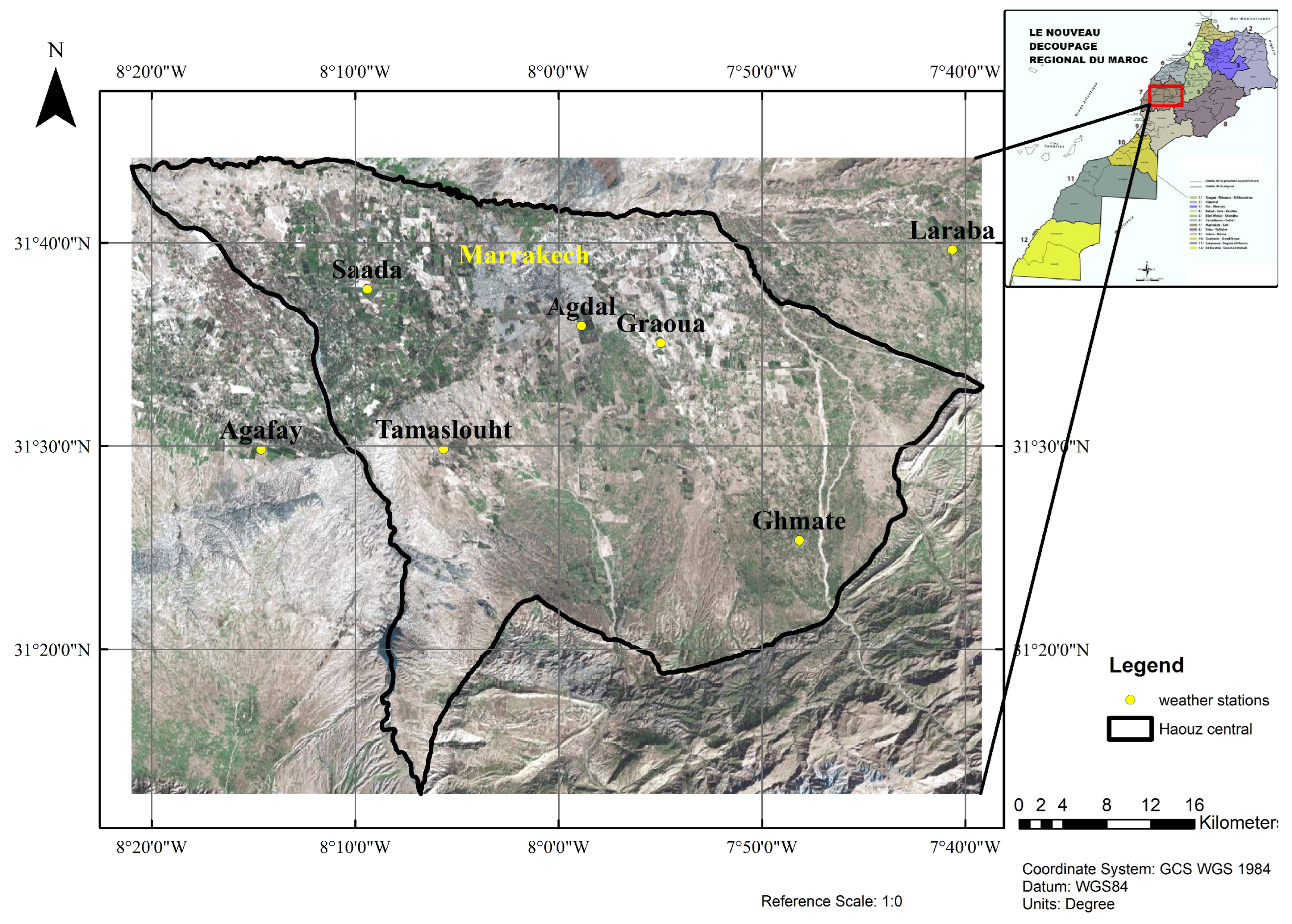
Figure 2.
Statistical metrics of the weathers stations compared to rainfall products in the study area – Daily time steps.
Figure 2.
Statistical metrics of the weathers stations compared to rainfall products in the study area – Daily time steps.
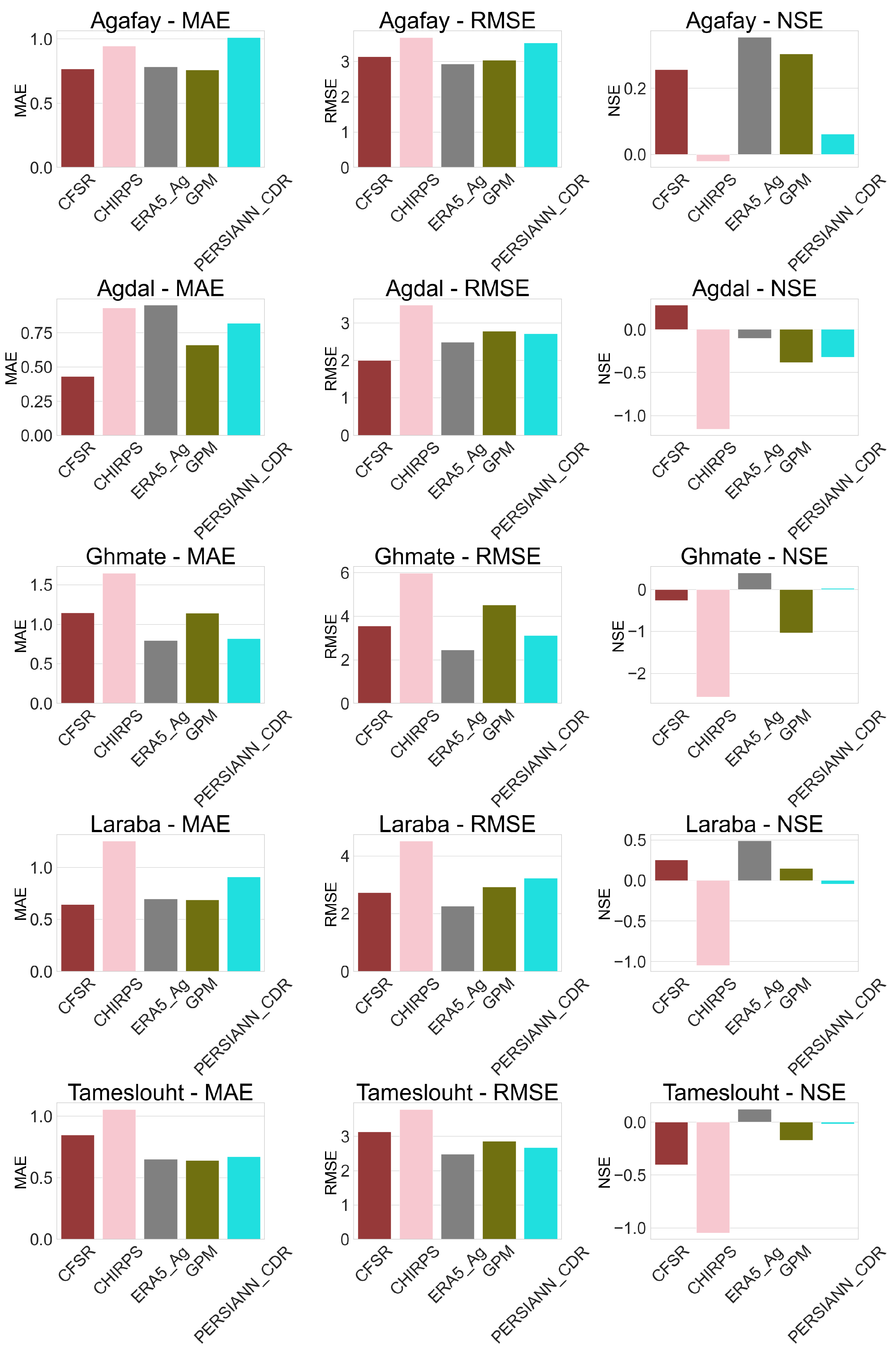
Figure 3.
Statistical metrics of the weathers stations compared to rainfall products in the study area – Monthly time steps.
Figure 3.
Statistical metrics of the weathers stations compared to rainfall products in the study area – Monthly time steps.
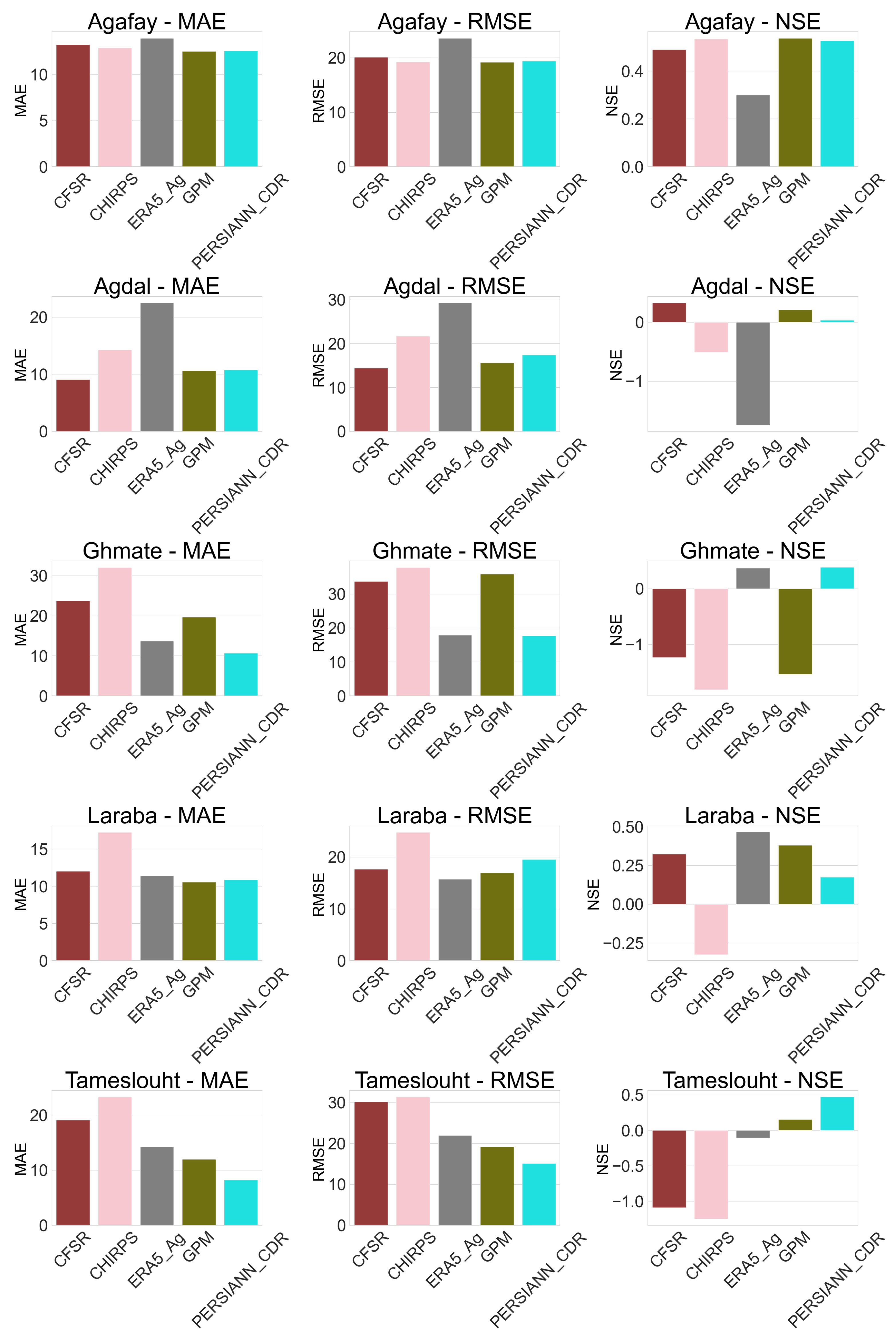
Figure 4.
Statistical metrics of the weathers stations compared to rainfall products in the study area – Annualy time steps.
Figure 4.
Statistical metrics of the weathers stations compared to rainfall products in the study area – Annualy time steps.
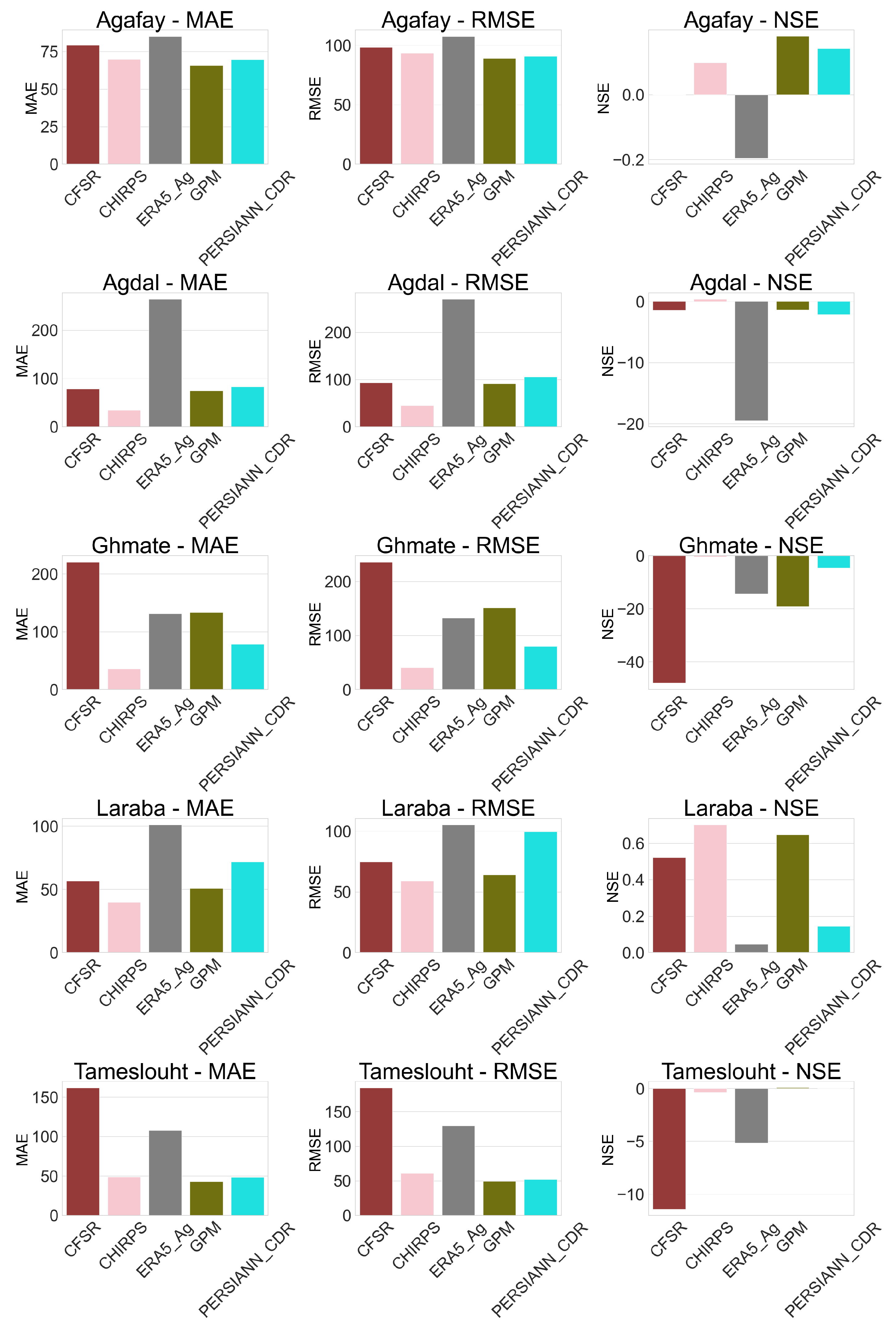
Figure 5.
Pearson correlation of precipitation products with ground-based stations across three time steps: daily, monthly, and yearly.(a) Daily, (b) Monthly, (c) Annualy.
Figure 5.
Pearson correlation of precipitation products with ground-based stations across three time steps: daily, monthly, and yearly.(a) Daily, (b) Monthly, (c) Annualy.
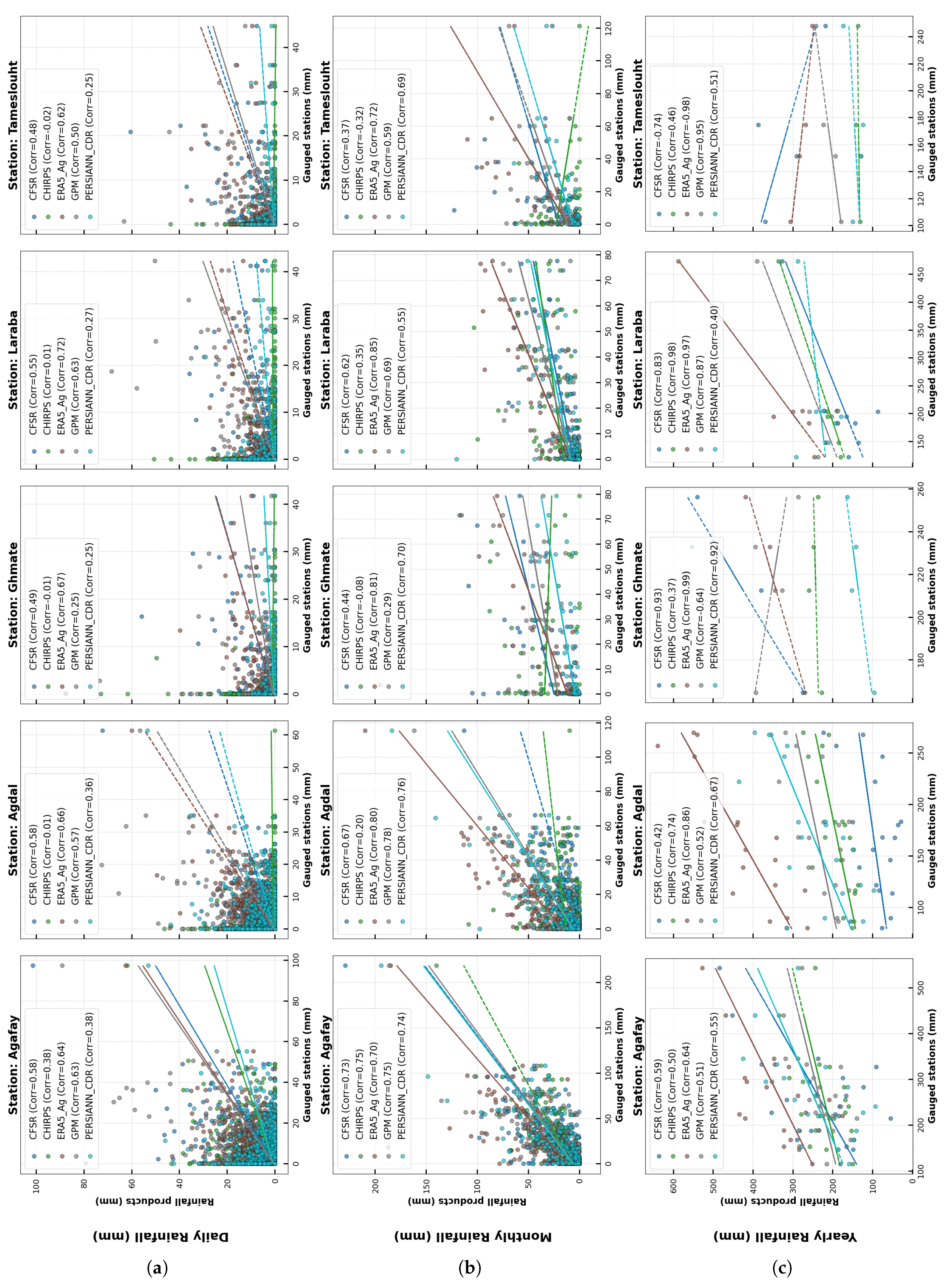
Figure 6.
Wavelet Power spectrum and scalograms - Yearly time scale at five gauged stations, red line refers to the global power spectrum of products where the dashed blue line refers to the one of gauged stations (a) Agafay station. (b) Agdal station, (c) Ghmate station, (d)Laraba station, (e)Tameslouht station.
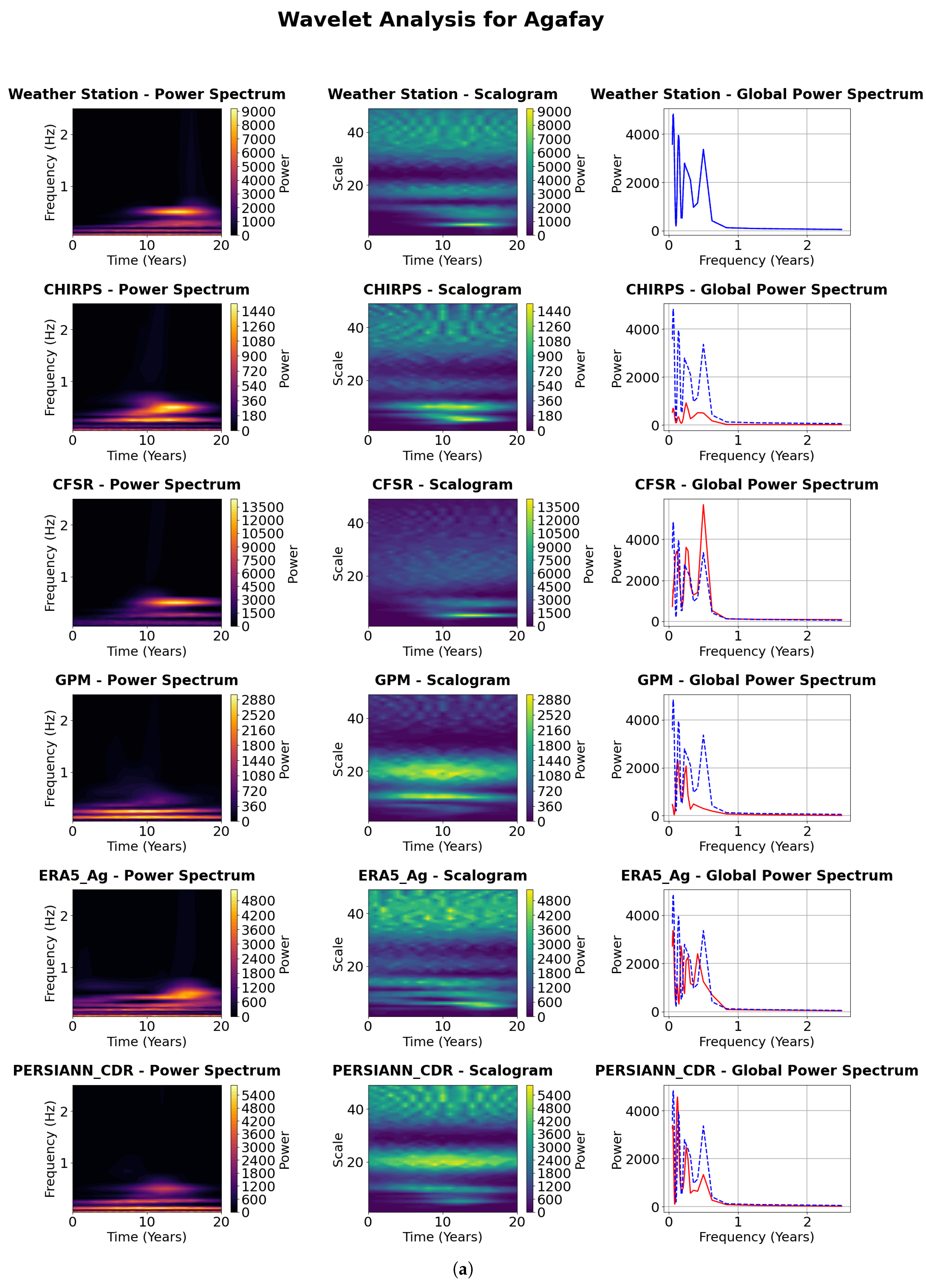
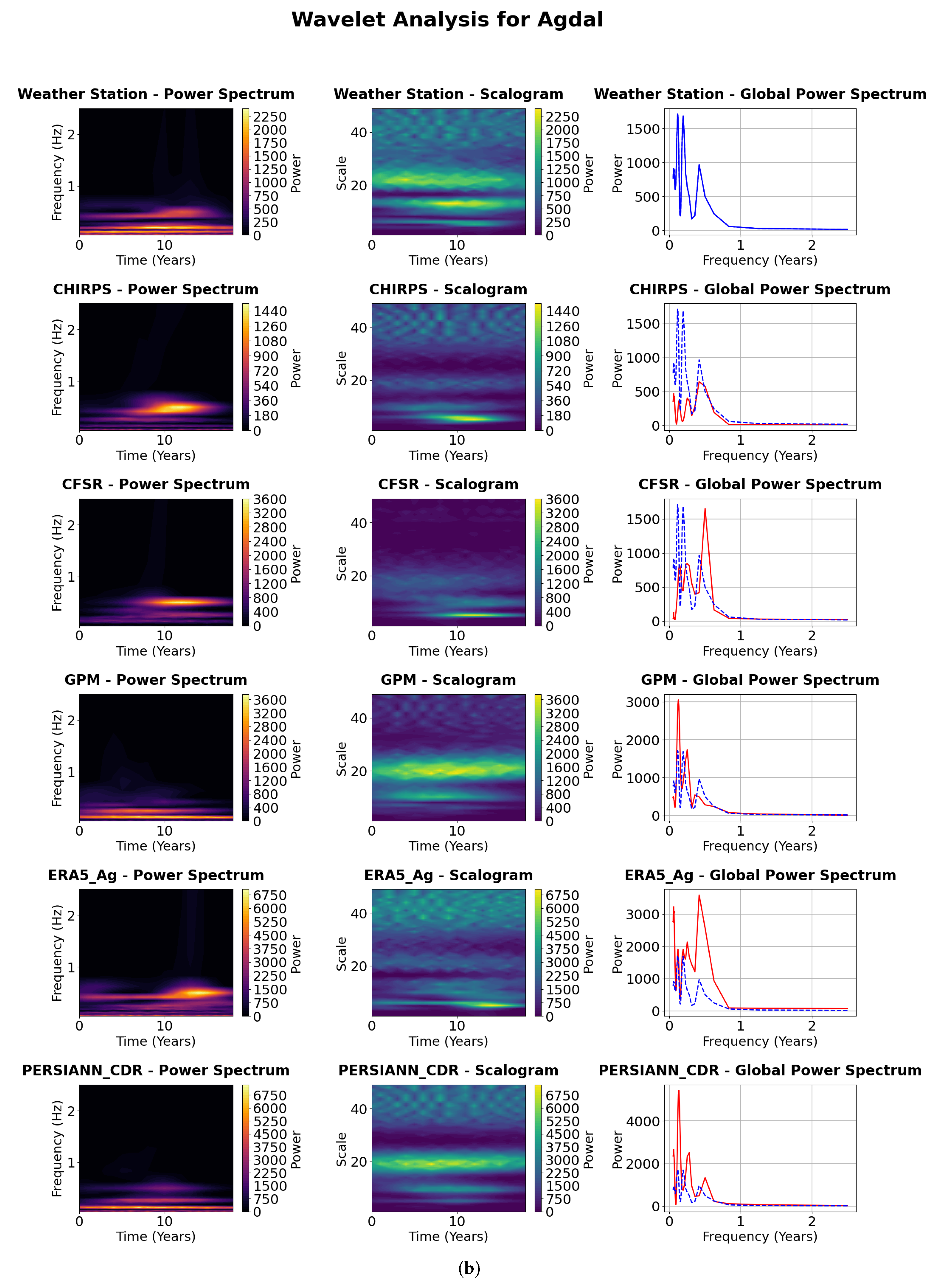
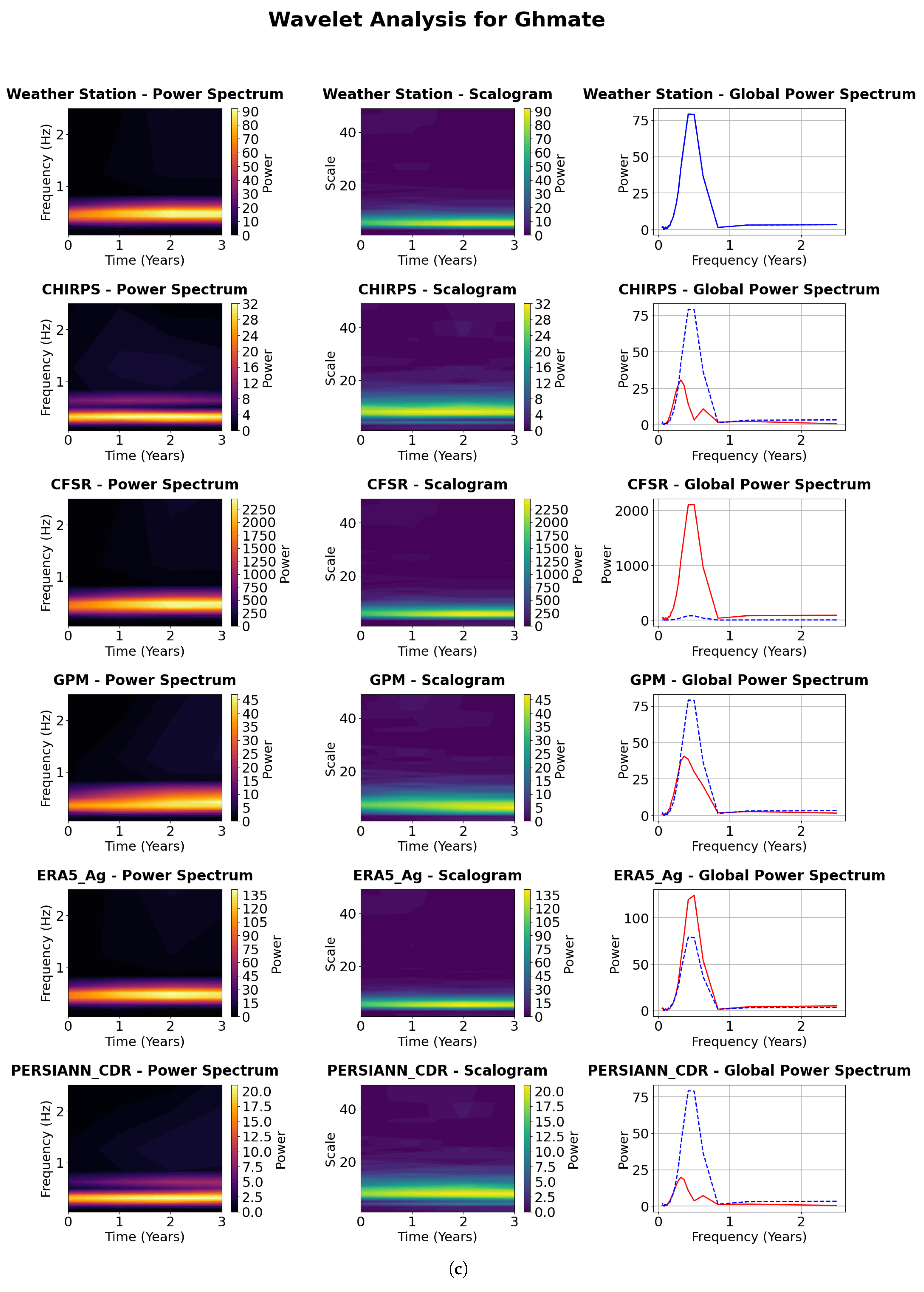
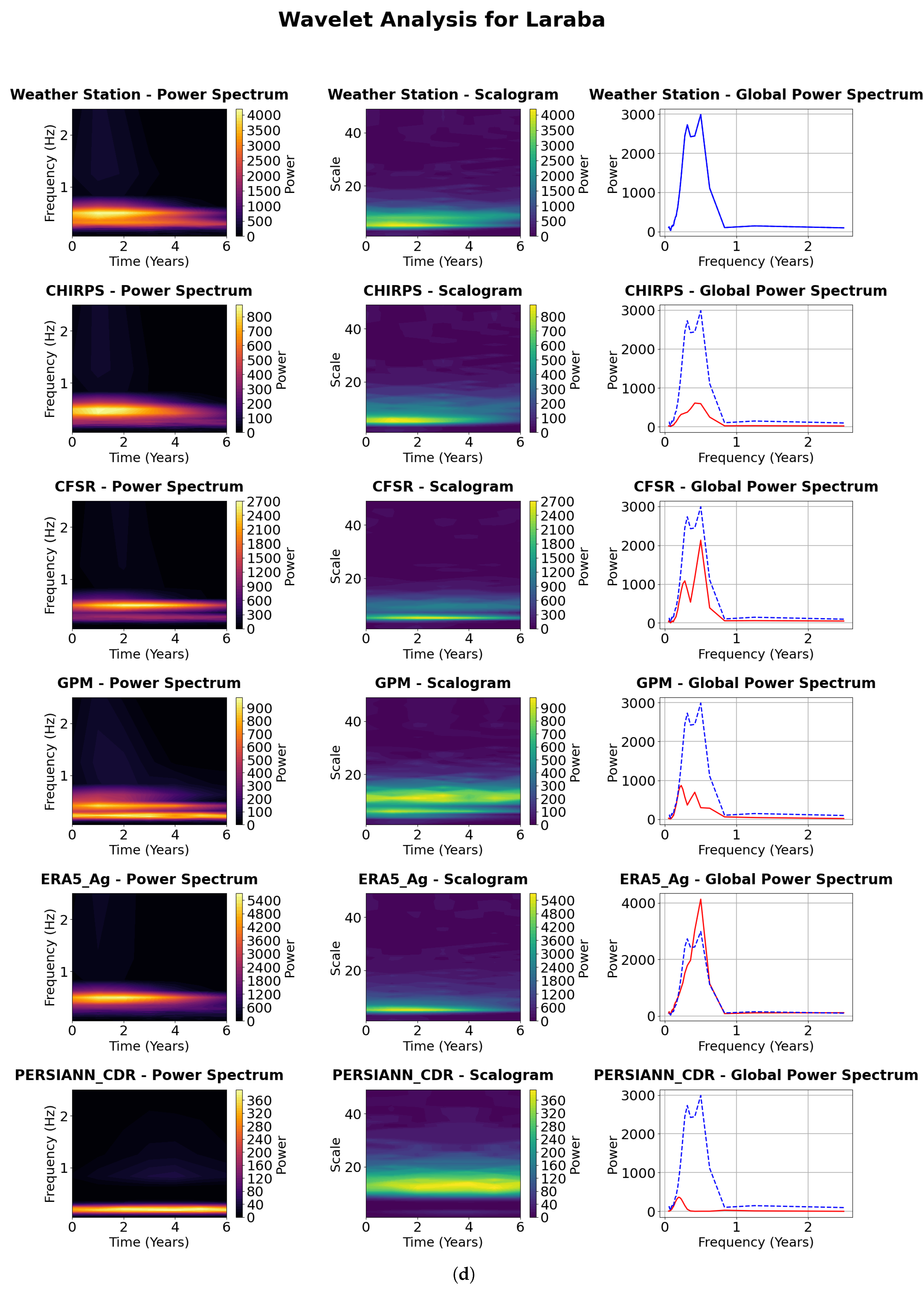
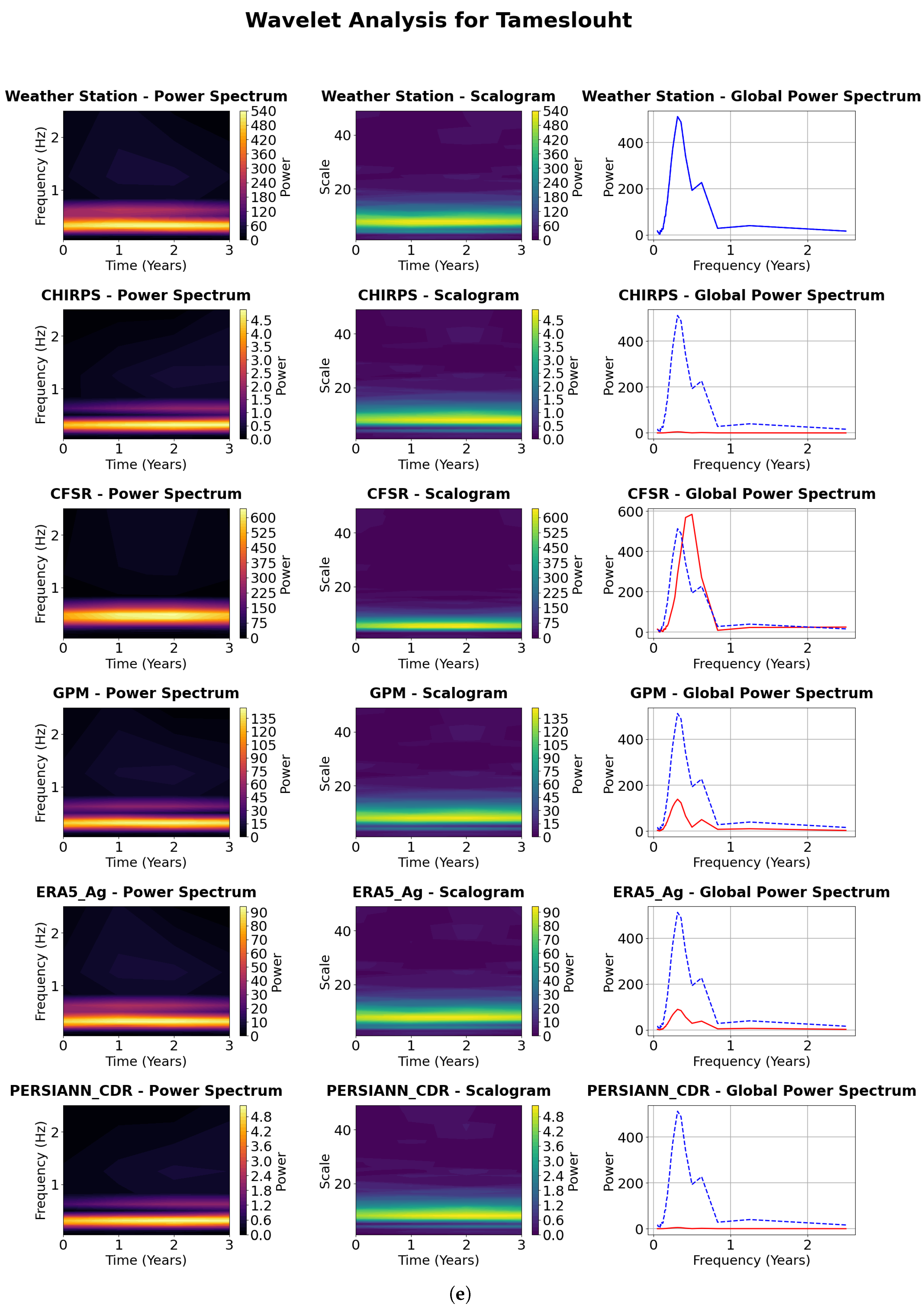
Figure 7.
Confusion matrix for different products and stations, dark green indicates a high value whereas light green indicates a low value. The overall structure of the confusion matrix is as follows: True Negatives (TN): “No Rain” correctly predicted (top left). False Positives (FP): “Rain” wrongly predicted (top right). False Negatives (FN): “No Rain” wrongly predicted (bottom left). True Positives (TP): “Rain” correctly predicted (bottom right), (b) Agafay station, (b) Agdal station, (b) Ghmate station, (b) Laraba station, (b) Tameslouht.
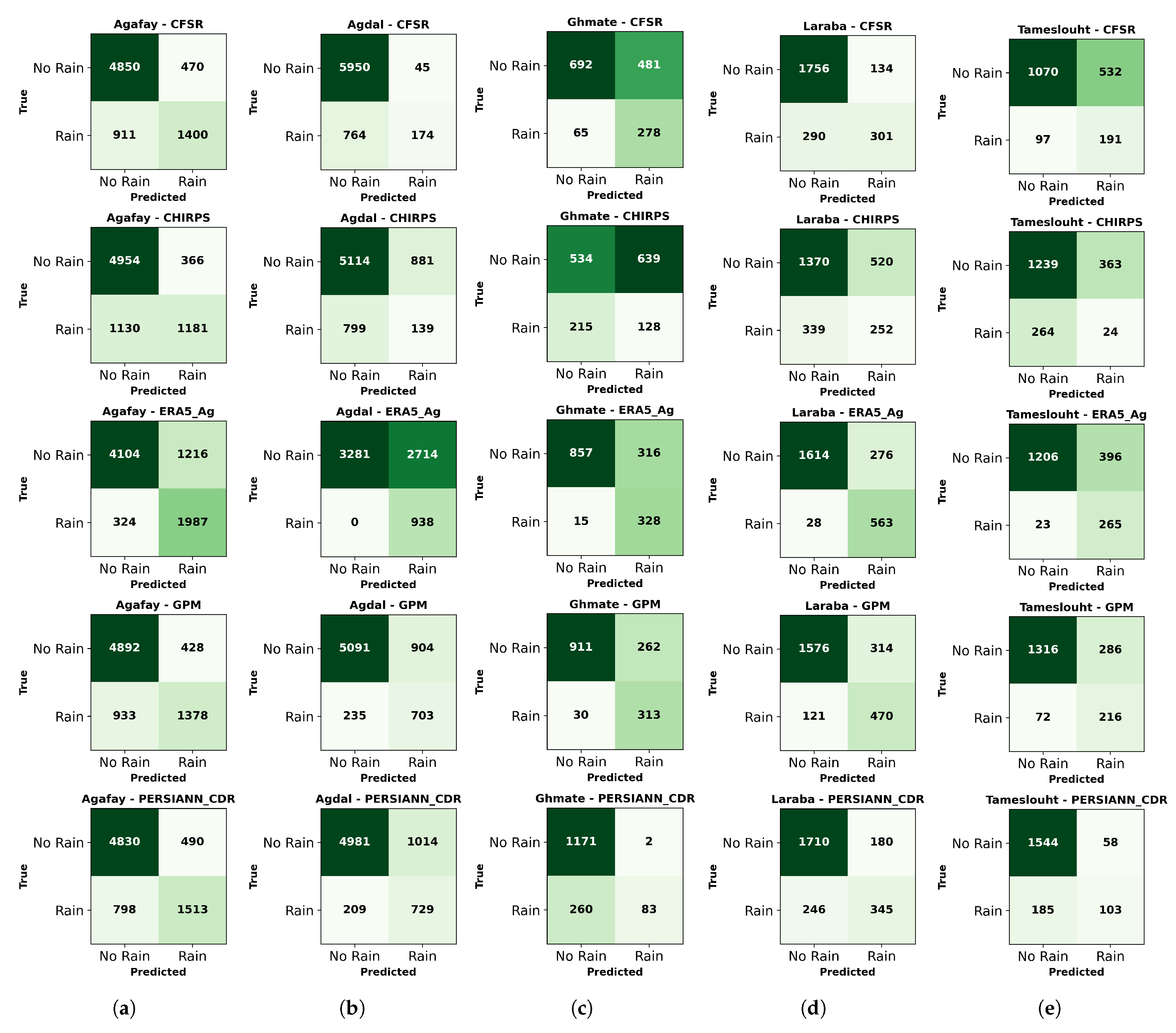
Figure 8.
Performance comparison of precipitation products based on several evaluation metrics.
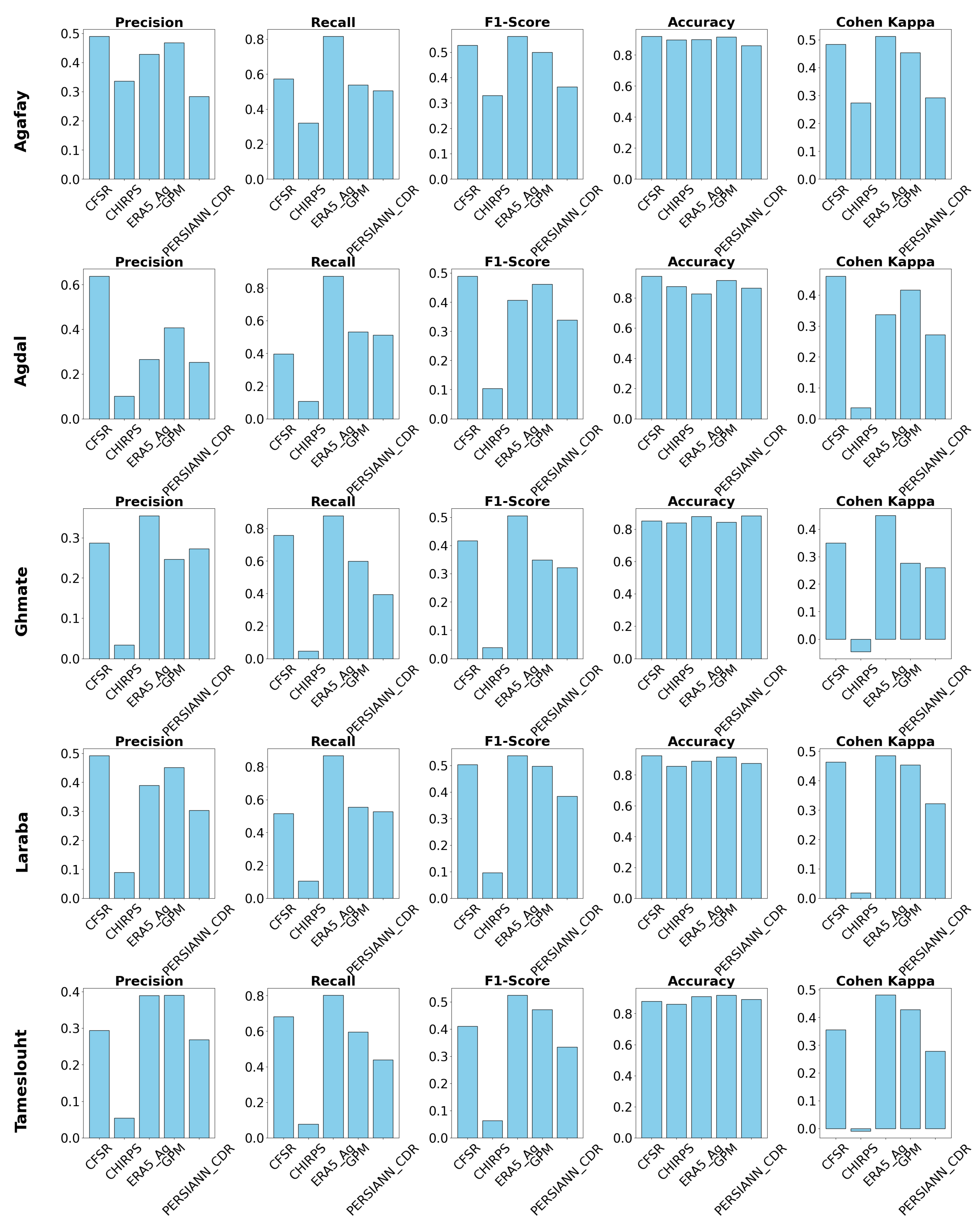
Figure 9.
precision-recall curve for different satellite and reanalysis products.
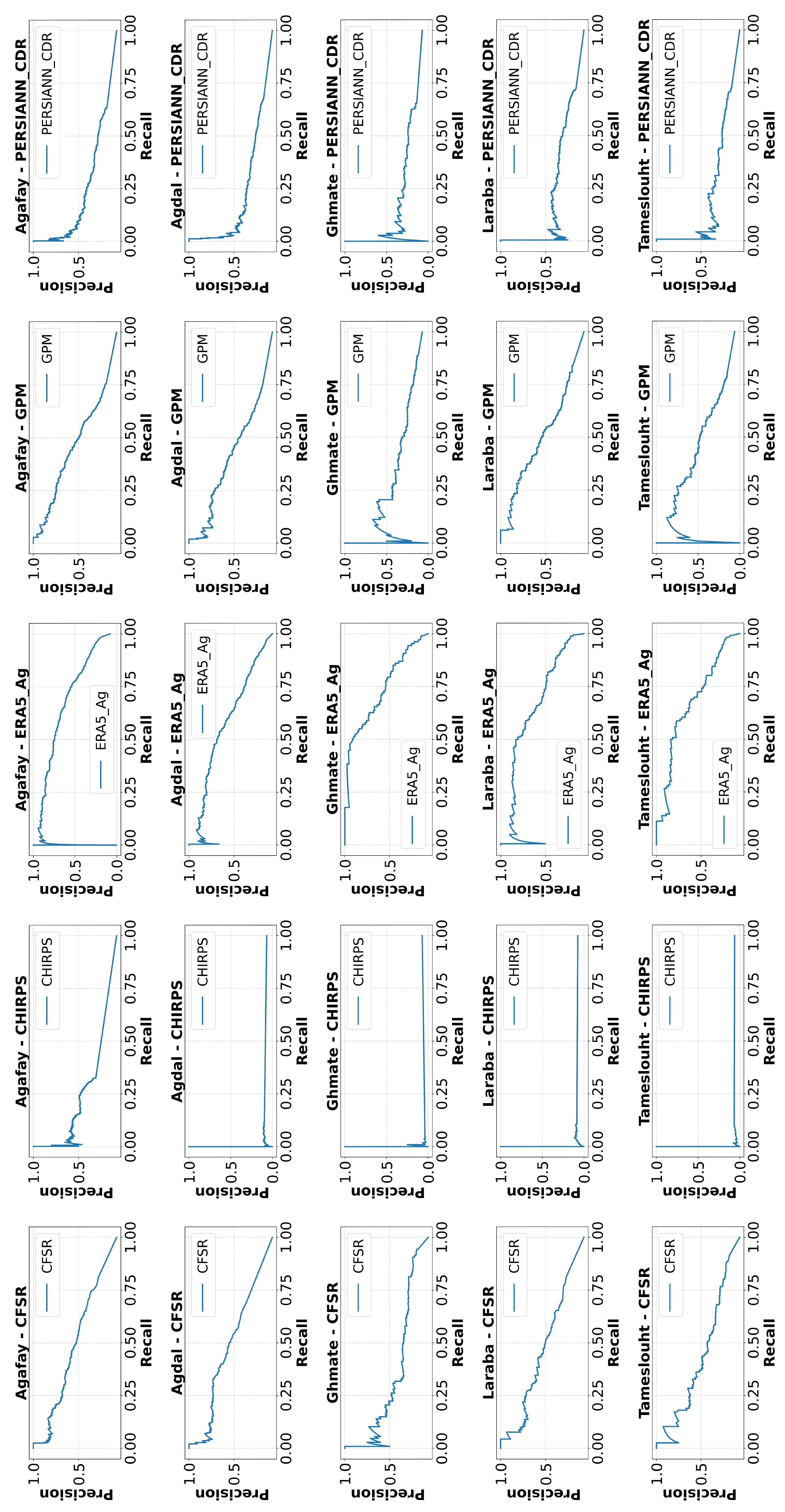
Figure 10.
Graphical illustration of bias evolution of raw and corrected data of rainfall products (ERA5_Ag and GPM), blue dashed lines indicate corrected data, yellow lines indicate raw data, (a) ERA5_Ag monthly scale, (b) GPM monthly scale, (c) ERA5_Ag Annual scale, (b) GPM Annual scale.
Figure 10.
Graphical illustration of bias evolution of raw and corrected data of rainfall products (ERA5_Ag and GPM), blue dashed lines indicate corrected data, yellow lines indicate raw data, (a) ERA5_Ag monthly scale, (b) GPM monthly scale, (c) ERA5_Ag Annual scale, (b) GPM Annual scale.
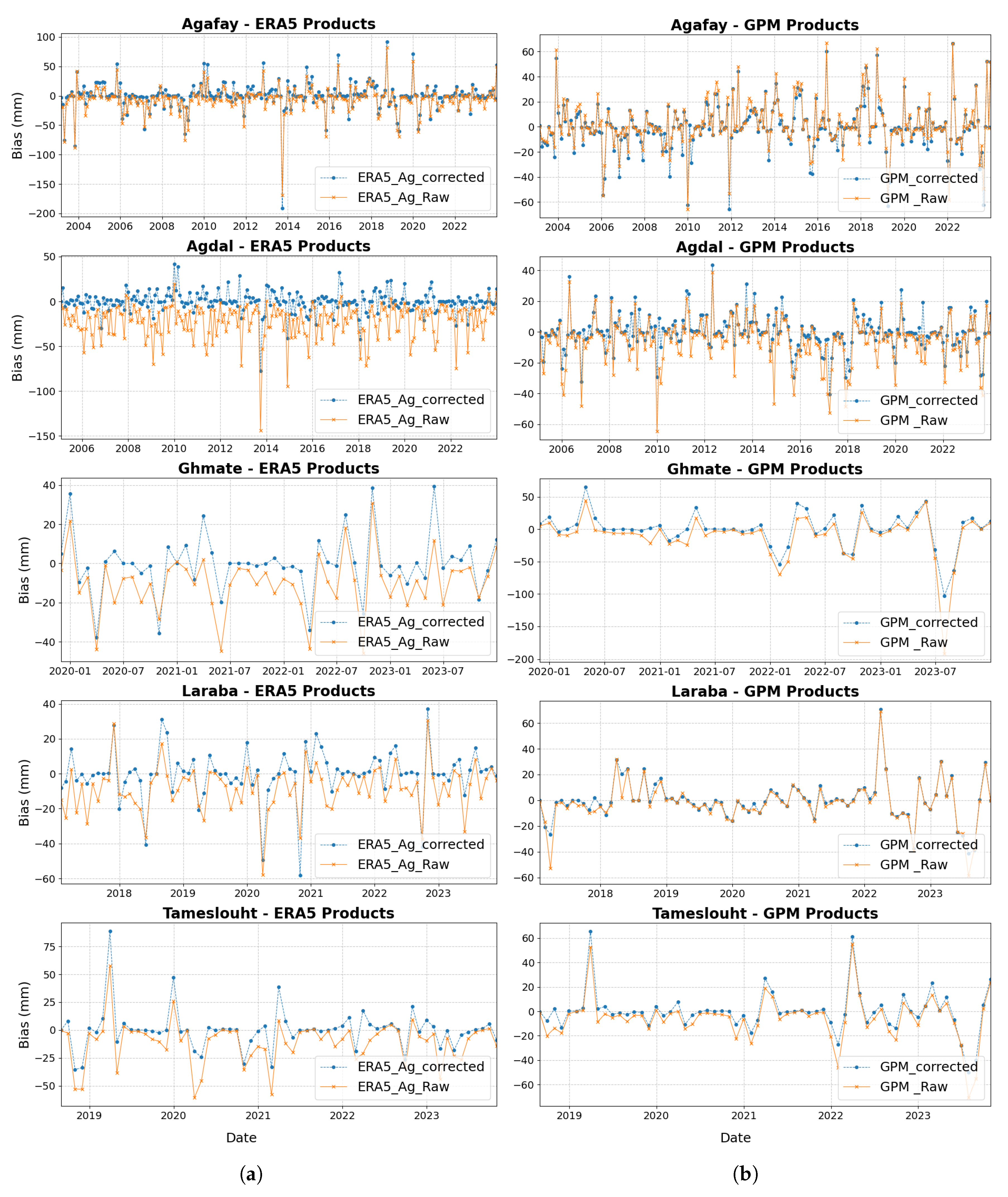
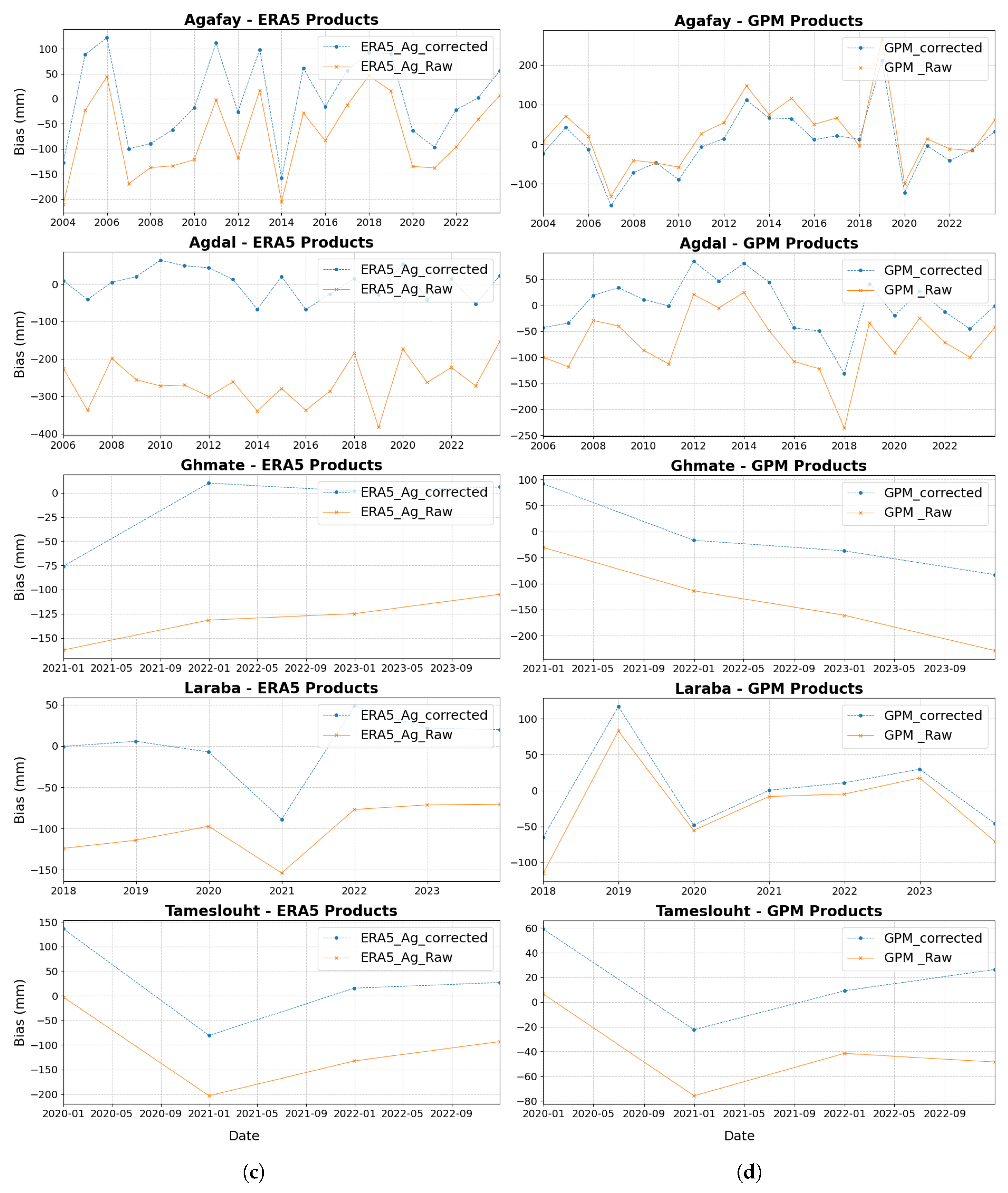
Figure 11.
Correlation graphs of precipitation data from rainfall products (ERA5_Ag and GPM) and weather station data at different time scales (daily, monthly and yearly). (a) Daily scale. (b) Monthly scale, (c) Annual scale.
Figure 11.
Correlation graphs of precipitation data from rainfall products (ERA5_Ag and GPM) and weather station data at different time scales (daily, monthly and yearly). (a) Daily scale. (b) Monthly scale, (c) Annual scale.
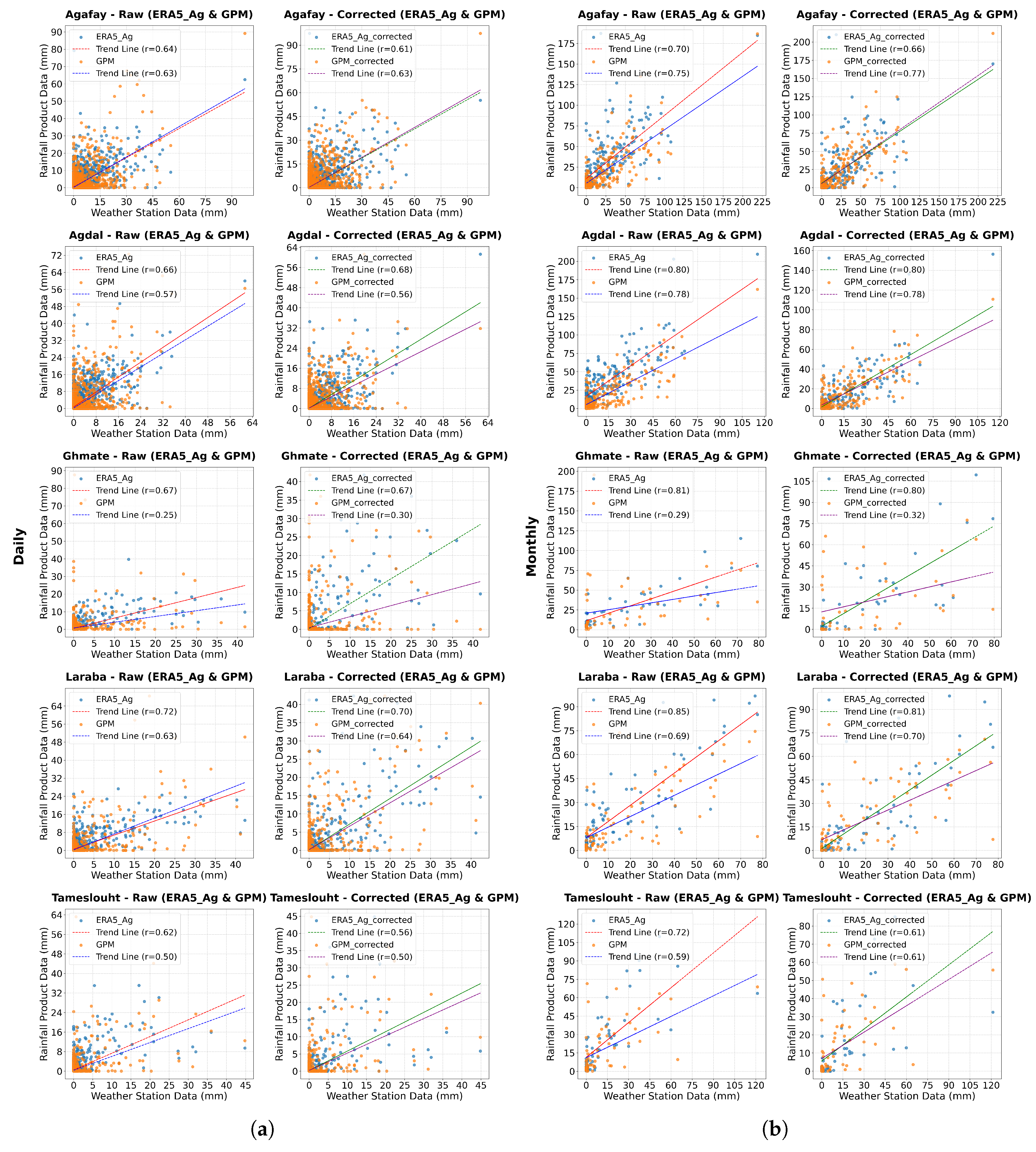
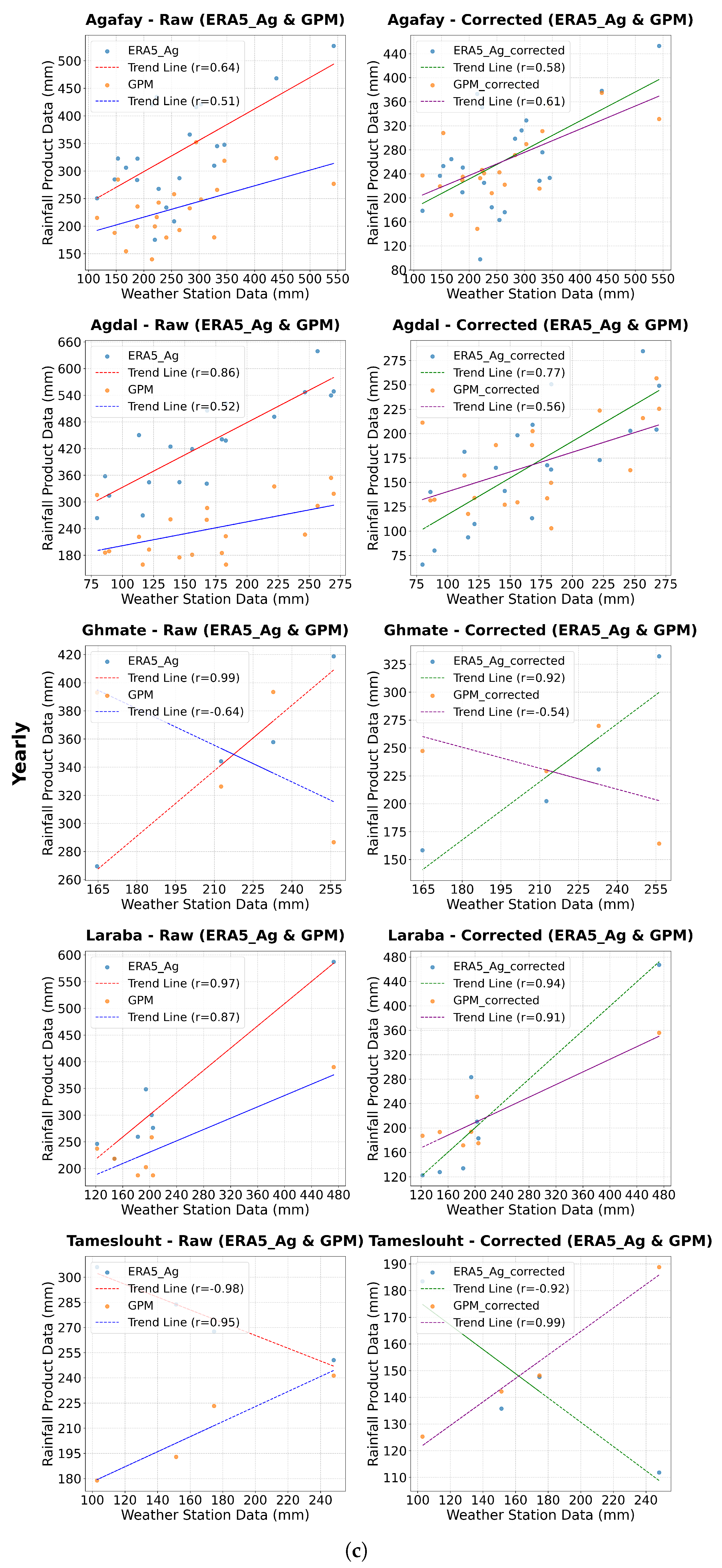
Figure 12.
CDF comparison of weather station data and rainfall products (ERA5_Ag and GPM) before correction and after correction.(a) Raw data, (b) Corrected data
Figure 12.
CDF comparison of weather station data and rainfall products (ERA5_Ag and GPM) before correction and after correction.(a) Raw data, (b) Corrected data
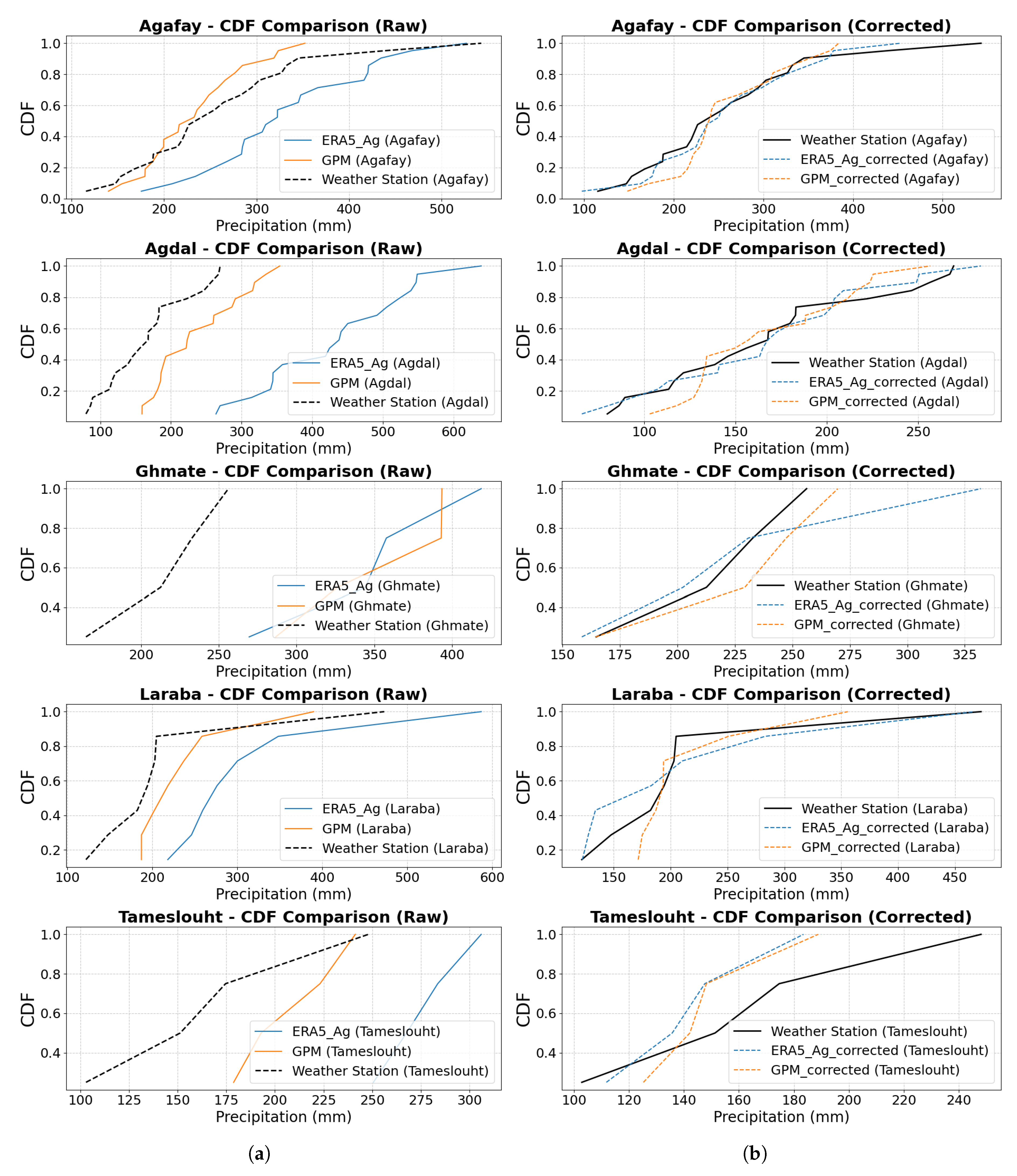
Figure 13.
Temporal Evolution of Precipitation : Comparison of Corrected ERA5_Ag and GPM Products with Measurement Stations, the black line represents the weather station, the dashed lines represent the corrected products (blue for ERA5_Ag and green for GPM), the red line corresponds to the raw ERA5_Ag product, and the light blue line corresponds to the raw GPM product, (a) monthly scale for ERA5_Ag, (b) yearly scale for GPM, (c) yearly scale for ERA5_Ag, (d) yearly scale for GPM.
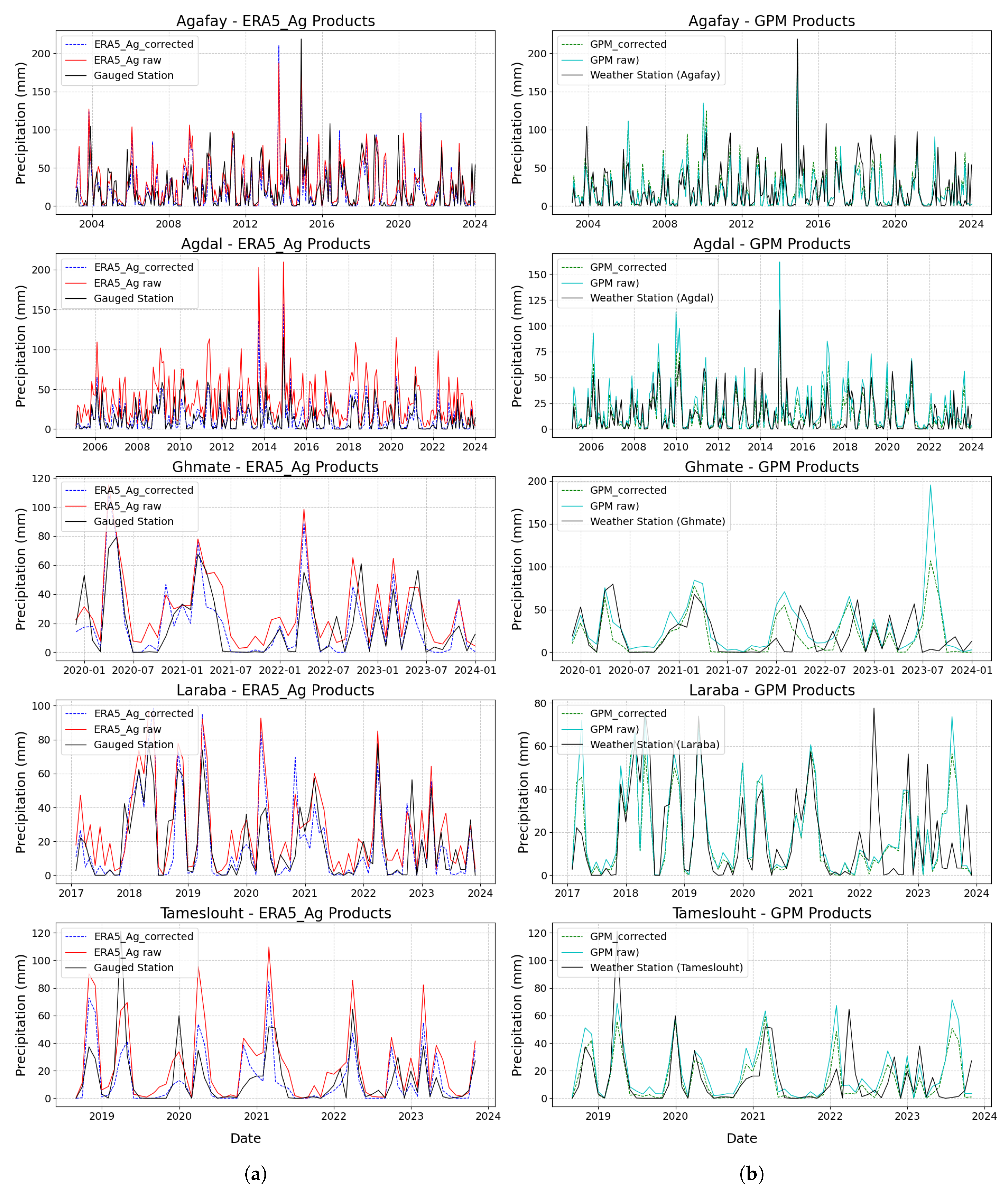
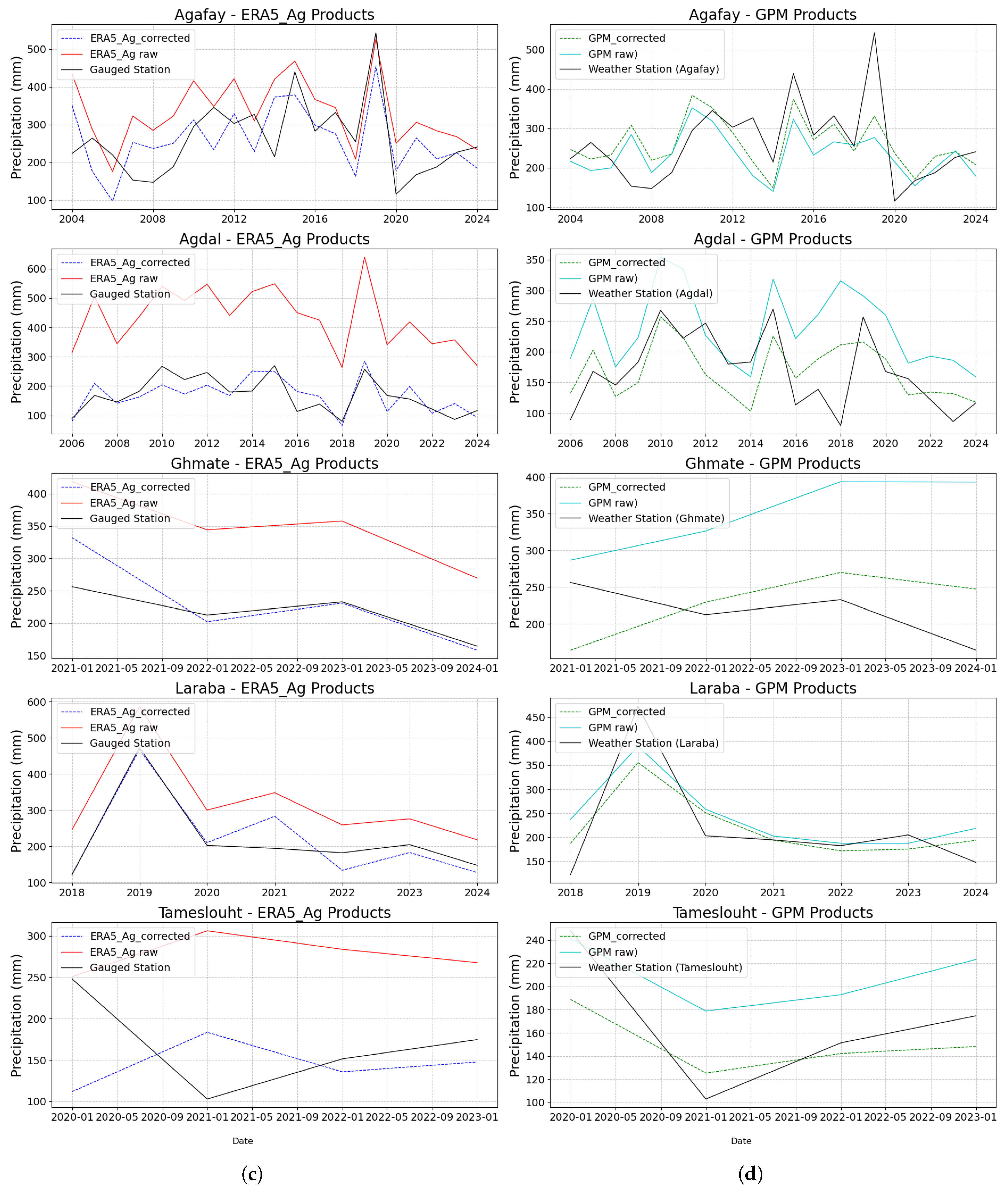

Table 1.
Characteristics of gauged stations in central Haouz plain.
| Station | X | Y | Altitude (m) | First Start-up Date | Frequency |
|---|---|---|---|---|---|
| Agafay | -8.24378 | 31.49711 | 479 | 2003-Present | 30 min |
| Agdal | -7.98143 | 31.59856 | 506 | 2004-Present | 30 min |
| Graoua | -7.91641 | 31.58444 | 523 | 2003-Present | 30 min |
| Ghmate | -7.80290 | 31.42273 | 761 | 2019-Present | 30 min |
| Laraba | -7.67748 | 31.66089 | 782 | 2017-Present | 30 min |
| Saada | -8.15673 | 31.62859 | 415 | 2022-Present | 30 min |
| Tameslouht | -8.09430 | 31.49745 | 554 | 2018-Present | 30 min |
All stations measure the following climatic variables: rainfall, temperature, wind speed, humidity and solar radiation.
Table 2.
Characteristics of gauged stations in central Haouz plain.
| Product | Spatial Resolution | Temporal Resolution | Time Span | Data Source | Coverage | Access Link |
|---|---|---|---|---|---|---|
| CHIRPS | 0.05° ( 5 km) | Daily, Monthly | 1981–present | Infrared satellite + gauge-based corrections | Global (50°S–50°N) | https://www.chc.ucsb.edu/data/chirps |
| ERA5-Ag | 9 km ( 0.08°) | Hourly, Daily | 1950–present | ECMWF reanalysis | Global | https://cds.climate.copernicus.eu/ |
| GPM | 0.1° ( 10 km) | Half-hourly, Daily | 2000–present | Multi-satellite + gauge correction | Global (60°S–60°N) | https://gpm.nasa.gov/data/directory |
| PERSIANN-CDR | 0.25° ( 25 km) | Daily | 1983–present | Infrared-based with machine learning corrections | Global (60°S–60°N) | https://www.ncei.noaa.gov/products/climate-data-records/precipitation-persiann |
| CFSR | 0.2° ( 20 km) | Hourly, Daily | 1979–2010 (Replaced by CFSv2) | NOAA NCEP Reanalysis | Global | https://rda.ucar.edu/datasets/ds093.0/ |
Table 3.
Characteristics of gauged stations in central Haouz plain.
| Metrics | Formulas | Interpretation |
|---|---|---|
| RMSE | Lower RMSE values indicate better model performance,while higher values indicate larger errors. | |
| MAE | A lower MAE indicates a better fit,while a higher MAE suggests a less accurate model. | |
| NSE | An NSE of 1 indicates perfect prediction. | |
| Bias | A bias close to 0 is ideal. | |
| Pearson Correlation | A value of 1 indicates perfect correlation. |
: estimated value. : Observed values. : Mean of observed values. : Mean of Estimated values. n: Total number of observations.
Table 4.
Confusion matrix forme.
| Estimated : Rainy | Estimated : Not rainy | |
|---|---|---|
| Observed : Rainy | True Positives (TP) | False Negatives (FN) |
| Observed : not rainy | False Positives (FP) | True Negatives (TN) |
Table 5.
Classification metrics used in this study.
| Metrics | Formule |
|---|---|
| Accuracy | |
| Precision | |
| Recall | |
| F1-Score | |
| Cohen’s Kappa |
TP (True Positives): Correctly detected rainy days, TN (True Negatives): Correctly detected dry days, FP (False Positives): Dry days incorrectly predicted as rainy, FN (False Negatives): Rainy days incorrectly predicted as dry
Table 6.
Wavelet parameters used for precipitation data analysis.
| Parameter | Value used | Description |
|---|---|---|
| Wavelet type | Cmor1-2.5 | Complex Morlet wavelet with parameters 1, 2.5 |
| Sampling period | Time step set to 1 year (data is annual). | |
| Wavelet scales | np.arange(1, 50) | Range of scales used for the Continuous Wavelet Transform (CWT). |
| Associated frequencies | Freqs (computed by PyWavelets) | Frequencies corresponding to the scales. |
| Detrending | Detrend(data) | Removal of the linear trend from the time series. |
Table 7.
Precipitation Bias Analysis.
| Gauged station | CFSR | CHIRPS | ERA5_Ag | GPM | PERSIANN_CDR | |||||
|---|---|---|---|---|---|---|---|---|---|---|
| A | M | A | M | A | M | A | M | A | M | |
| Agafay | -2.25 | -26.93 | -3.59 | -42.95 | 5.98 | 71.48 | -2.28 | -27.27 | -1.28 | -15.42 |
| Agdal | -5.92 | -71.06 | 2.12 | 25.42 | 21.98 | 263.77 | 5.83 | 69.97 | 6.66 | 80.03 |
| Ghmate | 16.89 | 168.91 | 13.04 | 130.49 | 9.79 | 97.91 | 10.04 | 100.40 | -7.13 | -71.33 |
| Laraba | -3.54 | -41.99 | 3.16 | 37.52 | 8.25 | 97.84 | 1.76 | 20.88 | -0.70 | -8.36 |
| Tameslouht | 12.97 | 136.25 | 5.49 | 57.72 | 10.63 | 111.71 | 5.19 | 54.54 | -0.70 | -7.38 |
M: Monthly, A: Annualy
Table 8.
Correlation coefficients of precipitation products with ground-based stations across three time steps: daily, monthly, and yearly.
Table 8.
Correlation coefficients of precipitation products with ground-based stations across three time steps: daily, monthly, and yearly.
| Station | CFSR | CHIRPS | ERA5_Ag | GPM | PERSIANN_CDR | ||||||||||
|---|---|---|---|---|---|---|---|---|---|---|---|---|---|---|---|
| D | M | Y | D | M | Y | D | M | Y | D | M | Y | D | M | Y | |
| Agafay | 0.58 | 0.73 | 0.59 | 0.38 | 0.75 | 0.50 | 0.64 | 0.70 | 0.64 | 0.63 | 0.75 | 0.51 | 0.38 | 0.74 | 0.55 |
| Agdal | 0.58 | 0.67 | 0.42 | 0.01 | 0.20 | 0.74 | 0.66 | 0.80 | 0.86 | 0.57 | 0.78 | 0.52 | 0.36 | 0.76 | 0.67 |
| Ghmate | 0.49 | 0.44 | 0.93 | -0.01 | -0.08 | 0.37 | 0.67 | 0.81 | 0.99 | 0.25 | 0.29 | -0.64 | 0.25 | 0.70 | 0.92 |
| Laraba | 0.55 | 0.62 | 0.83 | 0.01 | 0.35 | 0.98 | 0.72 | 0.85 | 0.97 | 0.63 | 0.69 | 0.87 | 0.27 | 0.55 | 0.40 |
| Tameslouht | 0.48 | 0.37 | -0.74 | -0.02 | -0.32 | 0.46 | 0.62 | 0.72 | -0.98 | 0.50 | 0.59 | 0.95 | 0.25 | 0.69 | 0.51 |
D: Daily, M: Monthly, A: Annualy
Disclaimer/Publisher’s Note: The statements, opinions and data contained in all publications are solely those of the individual author(s) and contributor(s) and not of MDPI and/or the editor(s). MDPI and/or the editor(s) disclaim responsibility for any injury to people or property resulting from any ideas, methods, instructions or products referred to in the content. |
© 2025 by the authors. Licensee MDPI, Basel, Switzerland. This article is an open access article distributed under the terms and conditions of the Creative Commons Attribution (CC BY) license (http://creativecommons.org/licenses/by/4.0/).
Copyright: This open access article is published under a Creative Commons CC BY 4.0 license, which permit the free download, distribution, and reuse, provided that the author and preprint are cited in any reuse.


